Quantum State Transfer via a Multimode Resonator

Abstract

Large-scale fault-tolerant superconducting quantum computation needs rapid quantum communication to network qubits fabricated on different chips and long-range couplers to implement efficient quantum error-correction codes. Quantum channels used for these purposes are best modeled by multimode resonators, which lie between single-mode cavities and waveguides with a continuum of modes. In this Letter, we propose a formalism for quantum state transfer using coupling strengths comparable to the channel’s free spectral range ($g{\sim}\Delta_{\text{fsr}}$). Our scheme merges features of both the STIRAP-based methods for single-model cavities and the pitch-and-catch protocol for long waveguides, integrating their advantage of low loss and high speed.

Practical quantum computation may require millions of qubits Fowler et al. (2012), while state-of-art technology holds only hundreds of qubits on a single superconducting processor  Castelvecchi (2023). Thus, it is necessary to network many processors by shuttling quantum information and distributing quantum entanglement Bravyi et al. (2022) using schemes of quantum state transfer (QST), in the same manner of quantum internet Kimble (2008); Wehner et al. (2018). To connect processors kept in the same or nearby dilution fridges, we expect the quantum links to range from centimeters to a few meters. We refer to this regime as medium range, in order to distinguish it from the cases of extremely short or long distances. This regime is also relevant to remote couplers that are necessary for quantum low-density-parity-check error-correction codes to significantly save the overhead of physical qubits Baspin and Krishna (2022); Bravyi et al. (2024). Although QST has been extensively studied in the past years Cirac et al. (1997); Christandl et al. (2004); Yao et al. (2005); Kay (2010); Korotkov (2011); Steffen et al. (2013); Wenner et al. (2014); Reiserer and Rempe (2015); Xiang et al. (2017); Vermersch et al. (2017); Axline et al. (2018); Kurpiers et al. (2018); Wang and Clerk (2012); Magnard et al. (2020); Burkhart et al. (2021); Bienfait et al. (2019); Zhong et al. (2021); Niu et al. (2023); Grebel et al. (2024); McKay et al. (2015); Sundaresan et al. (2015); Chakram et al. (2022); Chang et al. (2020), the medium-range QST needs to be revisited, for the following reasons.

As depicted in Fig. 1, the simplest setup of QST consists of two transmons qubits Koch et al. (2007) connected by a quantum channel. The channel supports standing waves with free spectrum range $\Delta_{\text{fsr}}$, which is reversely proportional to the channel length. To accurately model the system, one must compare the qubit-channel coupling strength $g$ with $\Delta_{\text{fsr}}$. For short-range channels where $\Delta_{\text{fsr}}\gg g$, only the mode closest to resonance is relevant. The channel is thus modeled by a single-mode cavity and QST with high fidelity is achieved by methods based on Stimulated-Raman-Adiabatic-Passage (STIRAP) Vitanov et al. (2017); Bergmann et al. (2019). For long-range channels where $\Delta_{\text{fsr}}\rightarrow 0$, the channel modes can be viewed as a continuum. In this case, QST is achieved by a propotal proposed by Cirac, Zoller, Kimble and Mabuchi (CZKM) Cirac et al. (1997), which is based on the input-output formalism and cascaded dynamics Gardiner (1993); Carmichael (1993). It is also referred to as the pitch-and-catch or relay method Zhong et al. (2019). The scheme consists of three steps: (1) pitch: qubit A emits a photon; (2) the photon flies to qubit B; (3) catch: B absorbs this photon.

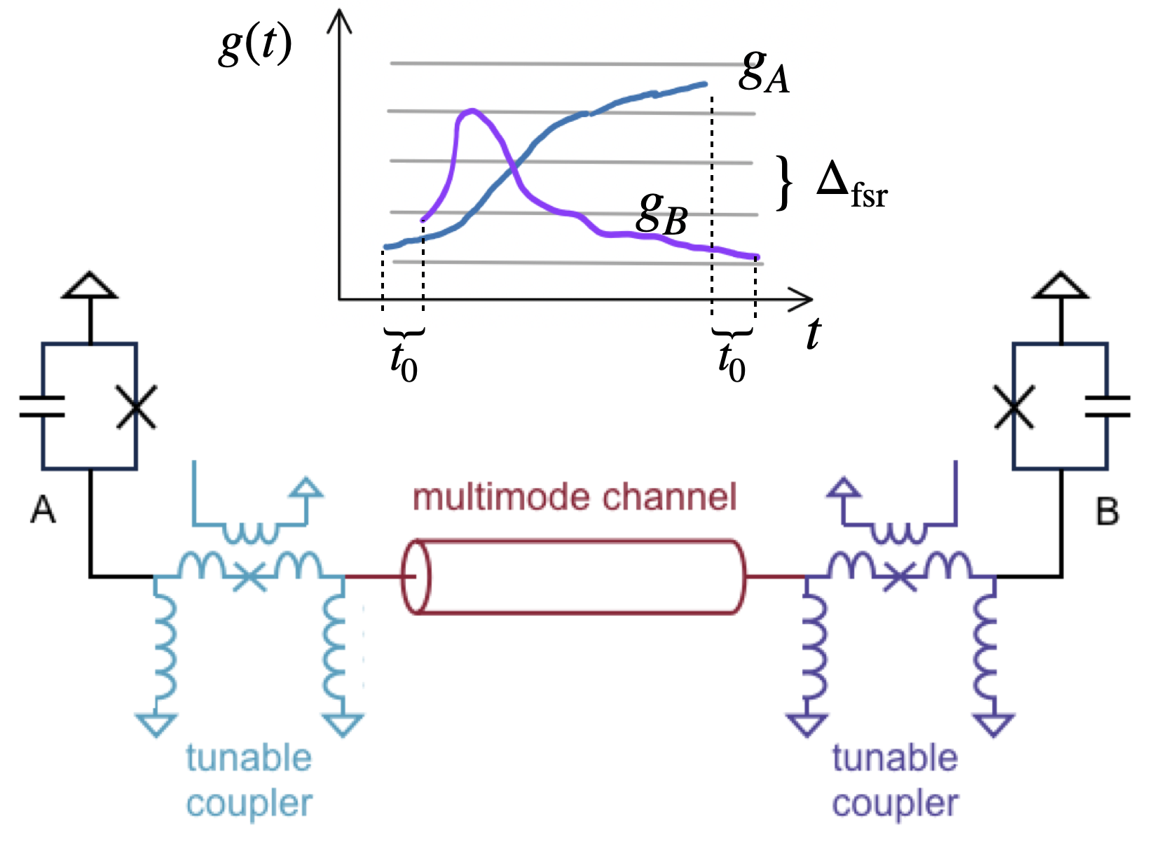
Figure 1: Schematic of the settings. Two qubits (labeled by A and B) are connected by a channel through two tunable couplers. The coupling $g_{A}(t)$ and $g_{B}(t)$ are activated sequentially with a delay of $t_{0}=\pi/\Delta_{\text{fsr}}$. Our scheme enables couplings with strength comparable with $\Delta_{\text{fsr}}$.

However, medium-range QST has not received sufficient theoretical attention despite emerging experiments McKay et al. (2015); Sundaresan et al. (2015); Chakram et al. (2022); Chang et al. (2020); Bienfait et al. (2019); Zhong et al. (2021); Niu et al. (2023); Grebel et al. (2024). Transmons-waveguide couplings typically have $g\lesssim 2\pi{\times}10^{2}\mathrm{MHz}$ Mirhosseini et al. (2019); Sheremet et al. (2023). A quick estimation shows that medium-range $\Delta_{\text{fsr}}$ is comparable to the attainable $g$, thus, the multiplicity and discreteness nature of the channel modes are both essential. For this regime, the old practice of CZKM and STIRAP are challenged. The CZKM scheme is questionable because the prerequisites of cascaded system and Markovian input-output formalism are inapplicable. To apply STIRAP-based methods, one has to suppress $g$ intentionally to prevent the involvement of multiple channel modes. However, weak couplings result in long scheme time, although a “hybrid” method employs STIRAP bright states to trade channel-loss-immunity for faster QST Wang and Clerk (2012); Bienfait et al. (2019); Zhong et al. (2021); Niu et al. (2023). Nevertheless, to operate QST in the regime of $g\sim\Delta_{\text{fsr}}$, a theory that extends beyond STIRAP and CZKM and coherently treats all the channel modes is needed.

In this Letter, we develop a formalism for medium-range QST. Our scheme reduces to STIRAP and the CZKM scheme at the short and long-range limits, respectively, consolidating their benefits of low loss and high speed from each of them. We notice that currently dynamics in the regime of $g\,{\sim}\,\Delta_{\text{fsr}}$ is also interested in other fields Krimer et al. (2014); Han et al. (2016); Johnson et al. (2019); Lechner et al. (2023); Lentrodt et al. (2023).

System and Model.

We study the settings outlined in Fig. 1, where two qubits (labeled by $A$ and $B$) are interconnected via a channel using two tunable couplers Chen et al. (2014). Here we focus on the essential physics, deferring all device-specific details to future works. The qubit has a transition frequency $\omega_{0}$, and the channel contains a set of equally-spaced (by $\Delta_{\text{fsr}}$) discrete levels with frequency $\{\omega_{k}\}_{k}$. The Hamiltonian under the rotating-wave approximation reads

$$H(t)= g_{A}(t)\hat{\sigma}_{A}^{\dagger}\sum_{k}\hat{c}_{k}e^{-i\delta_{k}t}$$ (1)

$$\quad+g_{B}(t)\hat{\sigma}_{B}^{\dagger}\sum_{k}(-1)^{k}\hat{c}_{k}e^{-i\delta_{k}t}+\text{H.c.}$$

where $\hat{\sigma}_{A/B}^{\dagger}$ is the qubit creation operator, $c_{k}$ denotes the channel annihilation operator, $\delta_{k}=\omega_{k}-\omega_{0}$, H.c. represents Hermitian conjugate, and the phase $(-1)^{k}$ in the second line reflects the distinct spatial profiles of even and odd channel modes Chang et al. (2020); Malekakhlagh et al. (2024). QST is described by the evolution of the state

$$\ket{\Psi(t)}=\alpha(t)\ket{1}_{A}+\beta(t)\ket{1}_{B}+\sum_{k}c_{k}(t)\ket{1}_{k},$$ (2)

where $\alpha(t)$, $\beta(t)$ and $c_{k}(t)$ are superposition coefficients and $\ket{1}_{A}$, $\ket{1}_{B}$ and $\ket{1}_{k}$ denote the state with a single excitation in qubit $A$, $B$, and mode $k$, respectively. The initial state has $\alpha(t_{i})=1$ and $\beta(t_{i})=c_{k}(t_{i})=0$. The target is to determine the profiles of $g_{A/B}(t)$ to achieve $\beta=1$ in the end.

To start, it is observed that A couples to a collective operator $\sum_{k}\hat{c}_{k}e^{-i\delta_{k}t}$ in $H(t)$, and the same operator couples to B in $H(t+t_{0}$) with $t_{0}=\pi/\Delta_{\text{fsr}}$, vice versa. This observation suggests delaying $g_{B}(t)$ relative to $g_{A}(t)$ by $t_{0}$, cf. Fig. 1, to ensure proper response of B to A. This retardation is further justified by causality: For standard waveguides where $\omega_{k}=k\Delta_{\text{fsr}}$ for all positive integer $k$, $t_{0}$ is exactly the time a photon takes to propagate from A to B. Henceforth, we introduce notations with a tilde to indicate a time reference shifted by $t_{0}$, e.g., $\tilde{\beta}(t)=\beta(t+t_{0})$ and similarly for others. We apply the convention that $g_{A}(t)=\tilde{g}_{B}(t)=0$ for $t<t_{i}$ and $t>t_{f}$, where $t_{f}$ marks the completion of control. This convention leads to a formula for $c_{k}(t_{f}+t_{0})$, or equivalently $\tilde{c}_{k}(t_{f})$ sp ,

$$\tilde{c}_{k}(t_{f})=-i\int_{t_{i}}^{t_{f}}d\tau\bigg{[}g^{*}_{A}(\tau)\alpha(\tau)+\tilde{g}_{B}^{*}(\tau)\tilde{\beta}(\tau)\bigg{]}e^{i\delta_{k}\tau},$$ (3)

where we have absorbed a factor of $e^{i\omega_{0}t_{0}}$ into the definition of $\tilde{g}_{B}$. QST is successful only if $\tilde{c}_{k}(t_{f})=0,\,\forall k$. Note that Eq. (3) vanishes as long as terms in the square bracket are orthogonal to $\exp{(i\delta_{k}\tau)}\,\forall k$ in the space of square-integrable functions over $\tau\in[t_{i},t_{f}]$. Thus, there is a huge degree of freedom for the options of the terms in the square bracket of Eq. (3). Among them, the most appealing choice might be

$$g^{*}_{A}(\tau)\alpha(\tau)+\tilde{g}_{B}^{*}(\tau)\tilde{\beta}(\tau)=0.$$ (4)

Equation (4) is reminiscent of the STIRAP dark state condition. We refer to it as the asynchronous dark state condition (ADSC) because the two terms therein are delayed by $t_{0}$. We find that ADSC implies the channel mode formula sp

$$c_{k}(t)=-i\int_{t-t_{0}}^{t}d\tau g_{A}^{*}(\tau)\alpha(\tau)e^{i\delta_{k}\tau},$$ (5)

and equations for the qubit amplitudes

$$\dot{\alpha}(t)=-g_{A}(t)\int_{t-t_{0}}^{t}d\tau K(t-\tau)g_{A}^{*}(\tau)\alpha(\tau),$$ (6a)

$$\dot{\tilde{\beta}}(t)=\tilde{g}_{B}(t)\int_{t}^{t+t_{0}}d\tau K(t-\tau)\tilde{g}_{B}^{*}(\tau)\tilde{\beta}(\tau),$$ (6b)

where $K(t-\tau)=\sum_{k}e^{-i\delta_{k}(t-\tau)}$.

These formulae display two notable features. Firstly, Eqs. (6a) and (6b) are formally decoupled. The interplay between the two qubits does not appear in the equations of motion, but is fully encoded in ADSC (4). We find it unusual, because when the system is not cascaded there are complex feed-back or forward written in the equations of motions, see for example Ref. Sinha et al. (2020); Zhang (2023). Secondly, we learn from the integral limits of Eqs. (5) and (6) that ADSC leads to a finite memory time bounded by $t_{0}$, irrespective of the system specifications.

Interpolation between STIRAP and CZKM.

Here we demonstrate that STIRAP and the CZKM scheme can be reproduced from our formalism. Immediately, taking the short-channel limit $t_{0}\rightarrow 0$ formally reduces Eq. (4) into the standard STIRAP dark state condition. Given that it is apparent, let us turn to emphasize the conceptional difference. STIRAP relies on the adiabatic approximation where diabetic error is unavoidable though can be suppressed Baksic et al. (2016); Malekakhlagh et al. (2024). This might be attribute to the fact that $t_{0}=0$ is the limit of $\Delta_{\text{fsr}}\rightarrow\infty$ where actually all channel modes are far blue detuned, thus, no effective coupling occurs. In contrast, we shall see that ADSC (4) can be rigorously satisfied.

The CZKM scheme Cirac et al. (1997) is cascaded setups and Markovian channels where $K(t)\propto\delta(t)$. Here the formal decoupling of Eqs. (6a) and (6b) is akin to cascaded dynamics and more interestingly, our ADSC-based formalism extends the validity of the CZKM scheme to quasi-long channels. Namely, if there are many discrete modes while $\Delta_{\text{fsr}}$ is not negligible, the kernel of the channel is approximated by Milonni et al. (1983)

$$K(t)\propto\lim_{N\rightarrow\infty}\sum_{k=-N}^{N}e^{-ik\Delta_{\text{fsr}}t}\propto 2t_{0}\sum_{n=-\infty}^{\infty}\delta(t-2nt_{0}),$$ (7)

The accuracy of Eq. (7) in approximating a real system may require further verification with the applied coupling strength. Nevertheless, only the term of $n=0$ in the summation survives when substituted into Eqs. (6). Thus, Eq. (6) is effectively Markovian, as same as in the CZKM formalism.

General Solutions.

Here we demonstrate that solutions of Eq. (6) satisfying ADSC do exist. As functions of time, $g_{A}(t)$ and $g_{B}(t)$ have infinitely many degrees of freedom. ADSC is a constraint that reduces these degrees of freedom by half. Thus, one strategy is to firstly freely choose an ansatz $g_{A}(t)$ and then find the corresponding $g_{B}(t)$. The key factor for this strategy to work is the formal decoupling of Eq. (6a) and Eq. (6b). To proceed, for any given $g_{A}(t)$, we substitute it into Eq. (6a) and obtain the trajectory $\alpha(t)$. We accept this $g_{A}(t)$ as long as $\alpha(t_{f})=0$ at some $t_{f}$ (or $\alpha\approx 0$ in practice, recall that exponential decay never reaches zero exactly). Suppose such a pair $[g_{A}(t),\alpha(t)]$ is obtained. The product $x(t)\equiv g_{A}^{*}(t)\alpha(t)$ is thus known and ADSC implies $\tilde{g}_{B}^{*}(t)\tilde{\beta}(t)=-x(t)$. Next, we define the abbreviation $y(t)\equiv-\dot{\tilde{\beta}}(t)/\tilde{g}_{B}(t)$ and obtained by

$$y(t)=\int_{t}^{t+t_{0}}d\tau\,K(t-\tau)x(\tau).$$ (8)

Then Eq. (6b) can be rephrased as

$$\tilde{\beta}^{*}(t)\dot{\tilde{\beta}}(t)=x^{*}(t)y(t),$$ (9)

The real part of Eq. (9) implies

$$\frac{d}{dt}\mathinner{\!\left\lvert\tilde{\beta}(t)\right\rvert}^{2}=2\,\mathrm{Re}\big{[}x^{*}(t)y(t)\big{]},$$ (10)

which completely determines the magnitude $|\tilde{\beta}(t)|$. Then, the imaginary part of Eq. (9) implies

$$\frac{d}{dt}\arg\tilde{\beta}(t)=\mathrm{Im}\big{[}x^{*}(t)y(t)\big{]}/\mathinner{\!\left\lvert\tilde{\beta}(t)\right\rvert}^{2},$$ (11)

which fixes the phase of $\tilde{\beta}(t)$. Now $\tilde{\beta}(t)$ is known and $\tilde{g}_{B}(t)$ is simply $-x(t)/\tilde{\beta}(t)$. One can verify the ADSC results by substituting the pair of $[g_{A}(t),\tilde{g}_{B}(t)]$ into the original Schrödinger equation.

In the end, the problem is reduced to the general existence of such $g_{A}(t)$ so that Eq. (6a) produces $\alpha(t_{f})\approx 0$ at some $t_{f}$. An example is sufficient to prove the existence. Let us consider the constant ansatz $g_{A}(t)=g$. [To satisfy ADSC, $g_{A}(t)$ must ramp up from zero. Constant $g$ is a good approximation if the ramping is quick.] We assume $t_{i}=0$ for brevity and apply Laplace transformation upon Eq. (6a) to obtain

$$\alpha(t)=\int_{\epsilon-i\infty}^{\epsilon+i\infty}\frac{e^{st}ds}{2\pi i}\bigg{[}s+g^{2}\sum_{k}\frac{1-e^{-(s+i\delta_{k})t_{0}}}{s+i\delta_{k}}\bigg{]}^{-1},$$ (12)

where $\epsilon>0$. We find that, due to the finite memory time $t_{0}$ of Eq. (6a), all the poles of the integrand have negative real parts sp . Thus, according to Cauchy’s residue theorem, $\alpha(t)$ is a sum of exponential decays that vanishes eventually.

To compare, if only qubit A is coupled to the channel, following the step of “pitch” of the CZKM scheme, the counterpart of Eq. (6a) will include the full history of $\alpha(t)$. Now all the poles of its Laplace transformation locate on the imaginary axis sp so that $\alpha(t)$ is a sum of harmonic oscillations.

Channel loss.

QST is affected by the losses from both the qubits and the channel. The former refers to the dissipation to environment other than the channel modes. We denote the qubit loss rate by $\gamma$ and the channel loss rate by $\kappa$. Generally we have $\gamma<\kappa$. Then, infidelity of QST caused by photon losses is estimated by $\gamma T+(\kappa-\gamma)\mathcal{E}$, where $T=t_{f}-t_{i}+t_{0}$ is the scheme time, and $\mathcal{E}$ is integrated channel population sp

$$\mathcal{E}\equiv \sum_{k}\int_{t_{i}}^{t_{f}+t_{0}}\,\mathinner{\!\left\lvert c_{k}(t)\right\rvert}^{2}dt$$ (13)

$$= t_{0}+\int_{t_{i}}^{t_{f}}\tau\frac{d}{d\tau}\big{[}\mathinner{\!\left\lvert\alpha(\tau)\right\rvert}^{2}+\mathinner{\!\left\lvert\tilde{\beta}(\tau)\right\rvert}^{2}\big{]}d\tau.$$

To protect QST from the losses, smaller $T$ and $\mathcal{E}$ are favored. It is conceivable that $T$ can be much smaller than the STIRAP-based methods because our scheme allows stronger couplings $g\sim\Delta_{\text{fsr}}$. For the channel loss, we find that $\mathcal{E}$ remains small for any realizations of $g_{A}(t)$ and $g_{B}(t)$ as long as ADSC is obeyed sp . Briefly, by substituting Eqs. (4) and (6) into Eq. (13), we find that the second term of Eq. (13) scales as $O(t_{*})$, where $t_{*}$ is the memory time of Eq. (6), i.e., the smaller one of $t_{0}$ (imposed by ADSC) and the intrinsic memory time determined by the kernel $K(t)$. For medium-range channels we have $t_{*}=t_{0}$, so that $\mathcal{E}=O(t_{0})$. Since $t_{0}$ is a small number in this regime, the channel loss is unlikely to be the bottleneck of fidelity.

Additionally, long-range channels have Markovian kernel ($t_{*}=0$) so that Eq. (13) reproduces the loss of flying photon $\mathcal{E}=t_{0}$. This is another evidence that CZKM can be derived from our formalism.

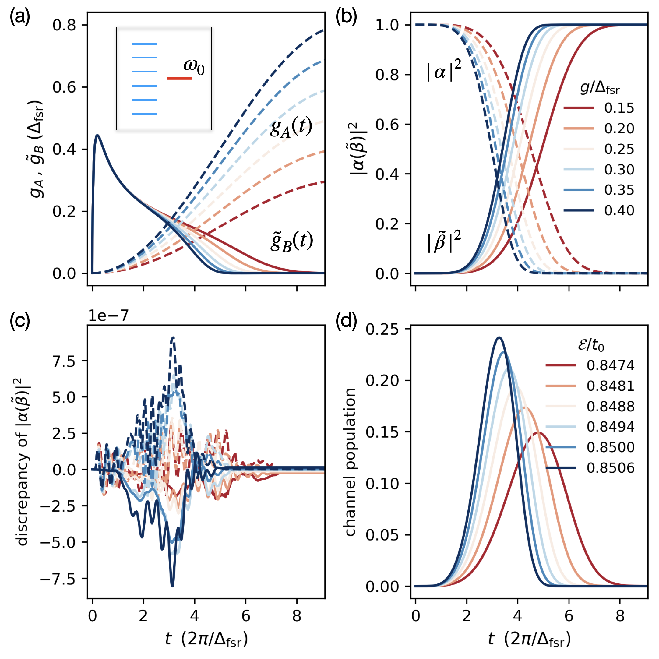
Figure 2: Numerical results for the setup with level structure depicted in the inset of (a), which contains six channel modes. (a) $g_{A}$ (dashed curves) and the companion $\tilde{g}_{B}$ (solid). (b) Qubit populations $\mathinner{\!\left\lvert\alpha\right\rvert}^{2}$ (dashed curves) and $|\tilde{\beta}|^{2}$ (solid curves) calculated from the original Schrödinger equation. (c) The discrepancies between the original Schrödinger equation and the ADSC-based equations: Dashed curves for $\mathinner{\!\left\lvert\alpha\right\rvert}^{2}$, and solid curves for $|\tilde{\beta}|^{2}$. (d) Channel populations and the table of the integrated population $\mathcal{E}/t_{0}$.

Examples.

As a demonstration of principle, we accommodate ourselves by considering two scenarios where the kernel $K(t-\tau)$, control pulses $g_{A/B}$ and amplitudes $\alpha(\beta)$ are all real-valued. In Case 1, $\omega_{0}$ is in the middle of two channel modes (detuned by $\pm\Delta_{\text{fsr}}/2$), see the inset of Fig. 2(a). In Case 2, $\omega_{0}$ is resonant with one channel mode, see the inset of Fig. 3(a). Each case involves an equal number of channel modes above and below $\omega_{0}$, set here to be three. We randomly choose $g_{A}(t)=g+g\sin[(t-5)/(10\pi)]$, where $g/\Delta_{\text{fsr}}=0.15\sim 0.4$ (in increments of 0.05, distinguished by colors) and $t$ denotes time in units of $2\pi/\Delta_{\text{fsr}}$ (thus $t_{0}=0.5$). Our computations utilize the Python IDEsolver package Karpel (2018) to solve Eq. (6a) and determine $\tilde{g}_{B}(t)$. We then validate the control pulses by solving the original Schrödinger equation using QuTiP Johansson et al. (2012, 2013), and compare the results of $\alpha(t)$ and $\tilde{\beta}(t)$ with the predictions of ADSC-based formulae. Numerical results for these two scenarios are shown in Figs. 2 and 3, respectively.

In Fig. 2(a) we plot the shapes of $g_{A}(t)$ (dashed curves) and the companion $\tilde{g}_{B}(t)$ (solid curves) obtained by the method introduced above. We then substitute the control pulses into the original Schrödinger equation and obtain the results of $|\alpha(t)|^{2}$ and $|\tilde{\beta}(t)|^{2}$ depicted in Fig. 2(b). The curves confirm that stronger $g_{A}$ facilitates faster QST. The results shown in Fig. 2(b) are compared with $|\alpha(t)|^{2}$ determined by Eq. (6a) and $|\tilde{\beta}(t)|^{2}$ calculated using Eq. (10). Their discrepancies are found to be smaller than $10^{-6}$, as plotted in Fig. 2(c). This error be further reduced by decreasing the temporal step length (set at $\Delta t=0.002$) in the numerical calculations. To assess the risk of channel loss, we plot the channel population $\sum_{k}\mathinner{\!\left\lvert c_{k}(t)\right\rvert}^{2}$ in Fig. 2(d), accompanied by the integrated population $\mathcal{E}$ (13) for each $g/\Delta_{\text{fsr}}$. The results corroborate our analysis that $\mathcal{E}=O(t_{0})$, and, somewhat surprisingly, $\mathcal{E}$ is almost invariant with respect to $g/\Delta_{\text{fsr}}$.

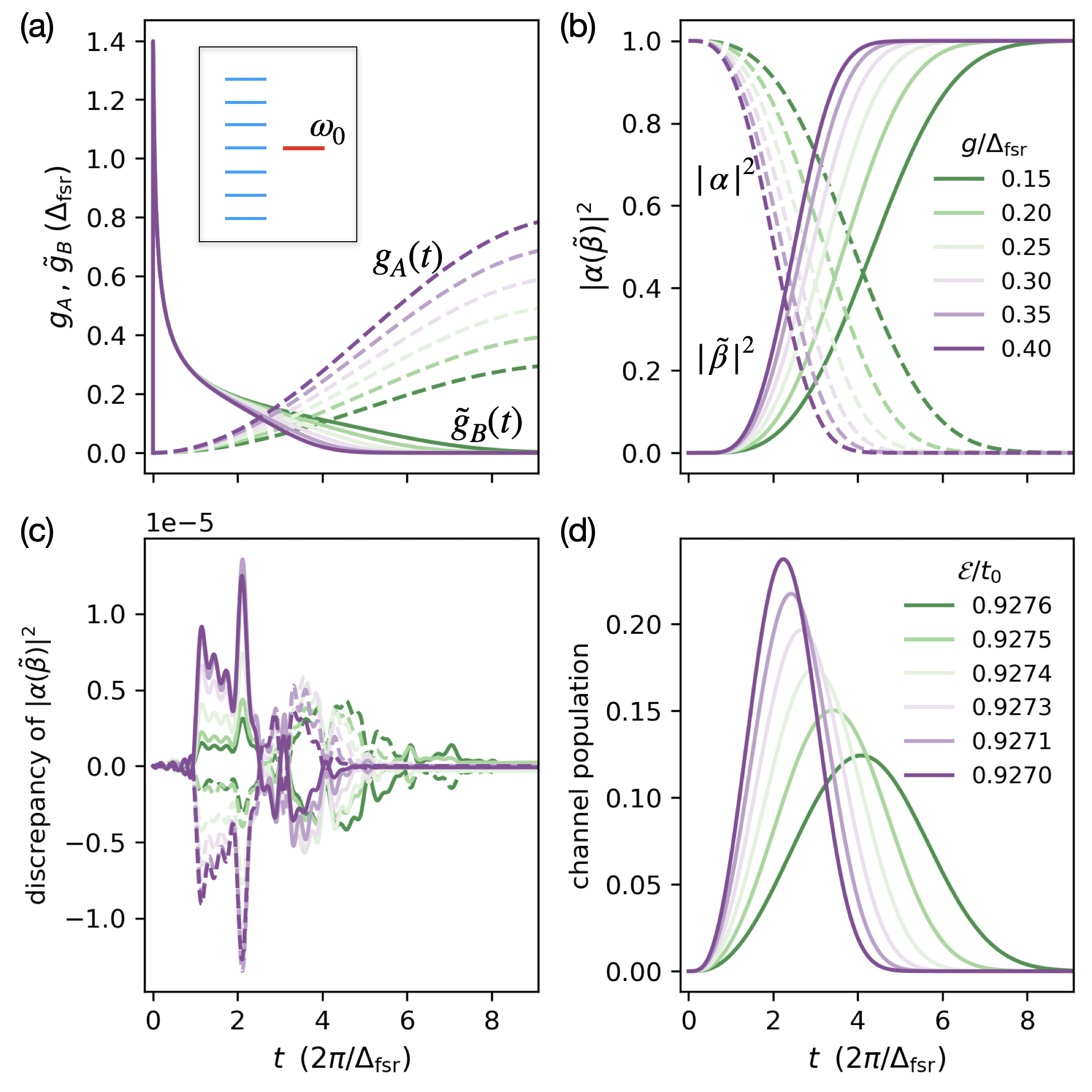
Figure 3: Numerical results for the setup with level structures depicted in the inset of (a), which contains seven channel modes. The subplots (a-d) are arranged in the same manner of Fig. 2.

Figure 3 conveys the similar message. Notably, the control sequences $\tilde{g}_{B}(t)$ shown in Fig. 3(a) exhibit higher peaks. The discrepancies between the full Schödinger equation and ADSC predictions are at the level of $10^{-5}$ (obtained with $\Delta t=0.001$), cf. Fig. 3(c). The integrated channel population is $0.927$ for all values of $g/\Delta_{\text{fsr}}$, exceeding than that observed in Fig. 2(d) by approximately 10%. This may elucidate the estimation that the level configuration of Case 2 yields higher fidelity Teoh (2023).

Conclusion.

In this Letter, we have developed a formalism for QST through a multimode channel. This central idea is to control the system time-dependently to satisfy ADSC (4). Our approach integrates key features of both STIRAP and the CZKM scheme, enabling QST implementation with coupling strengths comparable to the free spectral range of the channel $g\sim\Delta_{\text{fsr}}$. The increased coupling strengths give rise to faster QST, which is favored for minimizing qubit loss. Meanwhile, the risk of channel loss scales as $O(\kappa t_{0})$, where $t_{0}=\pi/\Delta_{\text{fsr}}$, independent of system specifications. The level of loss is acceptable because $t_{0}$ is typically much smaller than the QST scheme time. Our results have potential applications in the realization of fast and reliable chip-to-chip quantum communication, entanglement distribution, and couplers between non-neighboring qubits, which are crucial for large scale fault-tolerant quantum computation. For future works, one may propose other strategies for solving Eq. (6) and seek optimize the control pulses under realistic conditions. Remote quantum logic gates and frequency/time division multiplexing based on ADSC (4) might also be interesting topics.