TEAL: New Selection Strategy for Small Buffers
in Experience Replay Class Incremenal Learning

Abstract

Continual Learning is an unresolved challenge, whose relevance increases when considering modern applications. Unlike the human brain, trained deep neural networks suffer from a phenomenon called Catastrophic Forgetting, where they progressively lose previously acquired knowledge upon learning new tasks. To mitigate this problem, numerous methods have been developed, many relying on replaying past exemplars during new task training. However, as the memory allocated for replay decreases, the effectiveness of these approaches diminishes. On the other hand, maintaining a large memory for the purpose of replay is inefficient and often impractical. Here we introduce TEAL, a novel approach to populate the memory with exemplars, that can be integrated with various experience-replay methods and significantly enhance their performance on small memory buffers. We show that TEAL improves the average accuracy of the SOTA method XDER as well as ER and ER-ACE on several image recognition benchmarks, with a small memory buffer of 1-3 exemplars per class in the final task. This confirms the hypothesis that when memory is scarce, it is best to prioritize the most typical data.

1 Introduction

With the recent advances in deep neural networks, research interest in incremental learning has increased. Here, the problem of catastrophic forgetting, as defined by McCloskey and Cohen [20], can be severe. The necessity to incorporate new task knowledge into an already trained network has become more relevant given that training over extensive datasets is time-consuming. It is often impractical to retrain the network from scratch on the combined original and new task data. Furthermore, access to the already-trained data might be limited or non-existent.

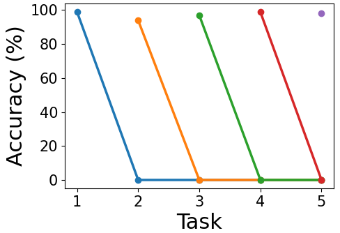
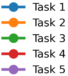
Figure 1: Catastrophic forgetting when training CIFAR-10 [13] sequentially with only finetuning.

Various methods have been developed to tackle this challenge across different frameworks, categorized by Van de Ven et al. [25] into three types: task-incremental, domain-incremental, and class-incremental learning. The core concept of incremental learning is that a model must learn tasks sequentially, one after another. Among these, class-incremental learning is considered the most challenging. In this scenario, each task introduces new classes, and the model must identify the specific class of each input without access to the task ID on which it was trained.

There are several approaches to incremental learning, each with its own distinct assumptions and configurations. In this paper, we adhere to the constrained setup described by De Lange et al. [7], which does not rely on task boundaries during training or testing. This setup maintains a constant memory size throughout incremental training, ensuring that it does not exceed a predetermined limit established at the outset. At each incremental step, we can add new exemplars to the memory buffer only after space has been allocated for them.

We focus our attention on a prevalent and rather successful framework called Experience Replay (ER), which involves storing a set of exemplars in memory and reusing them for rehearsal purposes while training on new tasks. Within this framework, several strategies exist for selecting which exemplars to retain in memory. Masana et al. [19] demonstrate that the most successful strategies are either random-sampling or Herding as defined by Welling [27]. Not surprisingly, the smaller the memory buffer is, the less effective the strategy is at mitigating catastrophic forgetting. This leads us to the following question: Are these strategies necessarily optimal for all memory sizes? In other words, could different strategies prove to be more effective depending on the size of the memory buffer?

Our proposed method, TEAL, operates on similar principles, aiming to identify a set of representative exemplars that also exhibit diversity. An exemplar is deemed representative if its likelihood, when considered within the distribution of all points in an appropriate latent space, is high. Leveraging clustering ensures the selection of a diverse set of exemplars. This approach enhances the model’s capacity to retain previous knowledge while effectively learning new tasks, even when constrained by a small memory buffer. Central to the success of this approach is our ability to derive an appropriate latent space. The subsequent sections elaborate on our methodology, experimental setup, comparative performance against alternative selection strategies, and the enhancements TEAL offers to various existing class-incremental methods.

Related work    Several approaches exist for incremental learning [see 7]. Alongside ER, alternatives include Generative Replay (GR) [23], Parameter Isolation, and Regularization. Similar to ER, GR replays data from previous tasks during new task training, but uses a generative model to create new samples instead of retaining exemplars seen by the model [6, 8, 9]. Parameter Isolation assigns distinct parameters to each task to reduce forgetting [18] by fixing parameters assigned to previous tasks, while Regularization-based methods [15] incorporate additional terms into the loss function to retain prior knowledge while learning from new data.

These methods differ in how they utilize memory: ER stores exemplars, GR stores a generative model, and Parameter Isolation stores task-specific parameters. Regularization-based methods do not rely on memory. This diversity makes it challenging to compare methods directly. In particular, we note that since generative models tend to be very large, this approach is hardly suitable to the domain of small memory buffers addressed below. Hence, our focus in this paper is on ER methods only.

Some CIL methods use an online learning setting, where each training example is seen only once. In this paper, we primarily use offline methods. Note that while few-shot incremental learning [24] may appear similar to our work on class-incremental learning (CIL) with a small memory buffer, there is a significant difference. We assume that the data for new tasks is initially sufficient for effective learning, whereas few-shot incremental learning inherently deals with a scarcity of labeled samples.

Summary of contribution    We present TEAL, a novel strategy designed to select effective exemplars for small memory buffers. TEAL can be seamlessly integrated with replay-based class-incremental learning methods, significantly enhancing their performance.

2 Problem formulation

CIL involves learning from a sequence of disjoint tasks, where each task requires the classification of a set of classes, and every class belongs exclusively to a single task. At each incremental step, the learner receives the data of the new task and, in some cases, has access to a memory buffer containing exemplars from previous tasks. After each step, the learner is tested on the successful classification of all the classes it has seen, including those seen in previous steps.

More formally [see 19], a class-incremental learning problem $\mathcal{T}$ consists of a sequence of $T$ tasks. Each task $t$ contains labeled samples from $n_{t}$ different classes $X^{1},\dots,X^{n_{t}}$, where $X^{i}=\{(x_{1},i),\dots,(x_{m^{i}},i)\}$. The tasks do not share classes, i.e., $X^{i}\cap X^{j}=\emptyset~{}\forall i\neq j$. We denote by $N^{t}$ the total number of classes in all tasks up to task $t$: $N^{t}=\sum_{i=1}^{t}{n_{i}}$.

We consider the scenario where there is access to a memory buffer ${\mathcal{M}}$, which has a fixed size throughout the learning of $\mathcal{T}$. An incremental learner is a learning model (we consider only deep neural networks) that is trained sequentially on the tasks. Accordingly, the training on task $t$ is performed on data $X^{1},\dots,X^{n_{t}},{\mathcal{M}}$, where ${\mathcal{M}}$ contains exemplars from tasks $1,\dots,t-1$.

Different CIL methods may employ different loss functions, but at test time, they are all required to classify a given example into its predicted class while considering all previously seen classes.

3 Our method: TEAL

In active learning, it has been shown (empirically and formally) that when the number of labeled examples is small, it is best to choose the most typical examples for training. In the context of CIL and when the memory buffer is too small to truly represent the distribution of each class, we propose to adopt this strategy for the selection of points that are intended to populate the replay memory buffer. In other words, when the buffer is considerably small, it should contain representative exemplars and thus retain a more significant fraction of the previously acquired knowledge.

Our proposed method TEAL, Typicality Election Approach to continual Learning, aims to address only one component of the general Incremental Learning (IL) problem, namely, how to populate the memory buffer at the end of each IL iteration. Accordingly, after task $t$, TEAL should select for each seen class $n=\frac{|{\mathcal{M}}|}{N_{t}}$ exemplars to populate memory buffer ${\mathcal{M}}$.

Ideally, any new mechanism for memory population can be combined with any competitive Experience-Replay-Incremental-Learning (ER-IL) method in which this mechanism is a separate module. In accordance, we evaluate TEAL by considering alternative ER-IL methods, where we replace their native mechanism for buffer population by our proposed method. In almost all cases, this mechanism involves random sampling from the known labeled set, in order to faithfully represent the class distribution. In our evaluation study, we also consider an alternative population mechanism called Herding [22, 12].

3.1 Description of method

We begin with a definition of point typicality.

Definition 3.1 (Typicality).

For each exemplar $x$, let

$$Typicality(x)=\left(\frac{1}{K}\sum_{x_{i}\in K\textrm{-}NN(x)}{\|x-x_{i}\|_{2}}\right)^{-1}$$

where $K$ is a fixed number of nearest neighbors.

The essence of TEAL  is to populate the memory buffer with points that are both typical (as captured by the definition above) and diverse.

After training on task $t$, the incremental learner has to update the memory buffer ${\mathcal{M}}$ with data from the new classes $\{X^{N^{t-1}+1},\dots,X^{N^{t}}\}$. Given the fixed size of ${\mathcal{M}}$, the learner must first reduce the number of exemplars already in the buffer to accommodate new ones from the new classes. For each class, this involves repeatedly removing examples from the buffer after each IL step.

To manage this, TEAL  maintains a list of the selected exemplars from each class ordered by typicality, reflecting the order in which they are to be deleted from ${\mathcal{M}}$. This allows the learner to remove the least typical points in the buffer, whenever new classes appear. To achieve this goal, whenever a new class is introduced, TEAL selects the initial set of representative exemplars through an iterative process. The selected list is ordered such that the most typical exemplars, which are to be retained for as long as possible, are positioned first, while those that will be removed first are positioned last.

More specifically, in each repeat of this iterative selection process and for each class separately, TEAL selects a small number of exemplars (a fraction of $n$, where $n$ denotes the number of exemplars assigned to the respective class). Let $S_{i}$ denote the set of exemplars after the $i^{th}$ iteration, for a total of $k$ iterations. Note that $S_{1}\subseteq S_{2}\subseteq\dots\subseteq S_{k}$ and that $|S_{k}|=n$. The sizes $|S_{1}|,\dots,|S_{k}|$ define the selection pace, indicating the pace of selecting exemplars from new class data.

To initialize the selection process, we need a suitable embedding space for the class exemplars. To this end we train a deep model on all the available training data, and use activations in its penultimate layer as a representation for the new classes [cf. 22]. Subsequently, the selection process in the $i^{th}$ iteration involves 2 steps (see pseudocode in Alg. 1):

Step 1: Clustering

Since typical examples tend to cluster in bunches [10], and in order to ensure diversity, we seek typical exemplars from different regions of the embedding space. We achieve this by dividing the set of labeled points into $|S_{i}|$ clusters, where $|S_{i}|$ represents the number of exemplars that should be selected from this class after the $i^{th}$ iteration.

Step 2: Typicality

We then select the most typical point from each of the $|S_{i}|-|S_{i-1}|$ largest uncovered clusters, where an uncovered cluster is a cluster from which no point has already been selected. We order the selected points by their typicality score.

  Input: $X^{c}$ COMMENT# a set of exemplars from class $c$

  Input: $n$ COMMENT# number of examples to choose

  Require: $\phi:{\mathcal{X}}\to{\mathbb{R}}^{d}$ COMMENT# current feature function

  Require: $s_{1},\dots,s_{k}$ COMMENT# iterations pace, $s_{1}\leq\dots\leq s_{k}=n$

  Output: ${\mathcal{M}}_{c}$ COMMENT# a set of n exemplars chosen from $X^{c}$

  $X^{c}_{emb}\leftarrow\phi(X^{c})$

  ${\mathcal{M}}_{c}\leftarrow\emptyset$

  for all $i=1,\dots,k$ do

     $C_{1},\dots,C_{s_{i}}\leftarrow$ clustering_algorithm$(X^{c}_{emb},\ s_{i})$ COMMENT# $|C_{1}|\geq\dots\geq|C_{s_{i}}|$

     for all $j=1,\dots,s_{i}-s_{i-1}$ do

        add $\underset{x\in C_{j}}{\mathrm{argmax}}\,\{Typicality(x)\}$ to ${\mathcal{M}}_{c}$

     end for

  end for

  return ${\mathcal{M}}_{c}$

Algorithm 1 TEALConstructExemplarSet

3.2 Using TEAL for incremental learning

The integration of TEAL into a general class-incremental algorithm is described in Algs. 2-3.

  Input: ${\mathcal{M}}_{c}=(m_{1},\dots,m_{|{\mathcal{M}}_{c}|})$ COMMENT# current exemplars set

  Input: $n$ COMMENT# number of examples to keep

  return $(m_{1},\dots,m_{n})$

Algorithm 2 ReduceExemplarSet

  Input: $X^{t}=\{X^{N^{t-1}+1},\dots,X^{N^{t}}\}$ COMMENT# training examples in per-class sets

  Require: $\theta^{t-1}$ COMMENT# current model parameters

  Require: ${\mathcal{M}}=({\mathcal{M}}_{1},\dots,{\mathcal{M}}_{N^{t-1}})$ COMMENT# current exemplar sets

  $\theta^{t}\leftarrow\textrm{training\_model}(X^{t},{\mathcal{M}};\theta^{t-1})$

  $n\leftarrow\frac{|{\mathcal{M}}|}{N^{t}}$ COMMENT# number of exemplars per class

  for $c\in\{1,\dots,N^{t-1}\}$ do

     ${\mathcal{M}}_{c}\leftarrow ReduceExemplarSet({\mathcal{M}}_{c},n)$

  end for

  for $c\in\{N^{t-1}+1,\dots,N^{t}\}$ do

     ${\mathcal{M}}_{c}\leftarrow ConstructExemplarSet(X^{c},n,\theta^{t})$

  end for

  ${\mathcal{M}}\leftarrow({\mathcal{M}}_{1},\dots,{\mathcal{M}}_{N^{t}})$

Algorithm 3 IncrementalTrain

4 Empirical evaluation

We report two settings: (i) Integrated:we evaluate the beneficial contribution of TEAL to competitive ER-IL methods, by replacing their native selection strategy with TEAL (Section 4.2.1); (ii) Alternative selection strategies:we evaluate the beneficial contribution of TEAL as compared to Herding (Section 4.2.2). In both cases, we incrementally train a deep-learning model with a fixed-size replay buffer and monitor the average accuracy defined below upon completion of each task $t$.

4.1 Methodology

The majority of the experiments are conducted using the open-source CL library Avalanche [16], with the exception of those involving XDER [1], which is not integrated into Avalanche. For XDER, we utilize the code provided by the authors. In order to guarantee a fair comparison and in all experiments, we employ identical network architectures and maintain consistent experimental conditions.

We make certain in both settings that the buffer remains class-balanced, namely, each update maintains an equal representation of exemplars across all classes. When the buffer size is not evenly divisible by the number of classes, there may be instances where certain classes possess one additional exemplar. To maintain this balance, we follow this procedure: Prior to adding new exemplars we calculate $n=\frac{|{\mathcal{M}}|}{N^{t}}$, where $N^{t}$ is the total number of existing and new classes. Subsequently, we adjust the number of exemplars from existing classes to accommodate $n$ by removing the least likely points, followed by the addition of $n$ exemplars from each new class.

In the second setting, we employ a simple baseline ER-IL model. This model updates a fixed-size buffer of exemplars after training each task $t$ and replays it while training on task $t+1$. Additionally, we utilize a weighted data loader to ensure a balanced mix of data from both the new classes and the exemplars stored in the buffer in each batch. Across experiments, the only variation lies in the selection strategy employed: some experiments utilize random-sampling, others utilize Herding, and the remaining experiments leverage TEAL. In some experiments, we replace the native buffer selection strategy of an existing ER-IL method with TEAL or Herding to assess their impact. Other than this change in the method’s buffer population mechanism, everything else remains the same.

Datasets    We use several well known Continual Learning benchmarks. (i) Split CIFAR-100[22, 5], a dataset created by splitting CIFAR-100 [13] into 10 tasks, each containing 10 different classes of 32X32 images, with 500 images per class for training and 100 for testing. (ii) Split tinyImageNet, a dataset created by splitting tinyImageNet [14] into 10 tasks, each containing 20 different classes of 64X64 images, with 500 images per class for training and 50 for testing. (iii) Split CUB-200[3], a dataset created by splitting the CUB-200 [26] high-resolution image classification dataset, consisting of 200 categories of birds, with around 30 images per class for training and 30 for testing.

Architectures    In the first setting, except for one experiment, we employ a ResNet-18 model in all our experiments. The exception is the experiment involving the training of XDER on the Split CUB-200 dataset. Due to computational limitations, we used instead a pre-trained ResNet-50 model [11], and this was maintained under all the relevant conditions. In the second setting, we use a smaller version of ResNet-18 [11] as a simple baseline ER-IL model [see 17].

Metrics    As customary, we employ a score that reflects the accuracy during each stage of the incremental training. Let $T$ denote the total number of tasks, and $a_{t,i}$ denote the accuracy of task $i$ at the end of task $t$ ( $i\leq t\leq T$). For every task $t={1,\dots,T}$, define it average accuracy $A_{t}=\frac{1}{t}\sum_{i=1}^{t}a_{t,i}$. This metric provides a single value for each incremental step, enabling us to directly compare different methods at each step. Since all of the experiments we conduct are task-balanced in the sense that each task has an equal number of classes, there is no need to add a weighting term to the metric.

Baselines    The following methods are suitable for our investigation as they are designed to address ER-IL: XDER [1] updates the memory buffer by adding current information to past memories and preparing the model for new tasks. ER-ACE [2], or ER with Asymmetric Cross-Entropy, uses a separate loss for new and past tasks. BiC [28] introduces a bias correction layer to address class imbalance in incremental learning. iCaRL [22] combines the incremental classifier and representation learning with a nearest-mean-of-exemplars strategy, and Herding for exemplar selection. Since the classifier is based on the nearest-mean-of-exemplars, Herding is crucial for the selection strategy, as it guarantees that the features of the exemplars in the buffer approximate the original classes means. GEM [17] uses Gradient Episodic Memory to prevent gradient leakage between new and past tasks through constrained optimization. GDumb [21] employs a greedy sampling strategy for memory storage and retrains the neural network from scratch during inference. ER [4] explores different selection strategies in a simple ER framework.

In order to evaluate the competitiveness of these methods, we conducted multiple runs on Split CIFAR-100, utilizing fixed buffer sizes of 300, 500, and 2000. Fig. 2 shows the results.

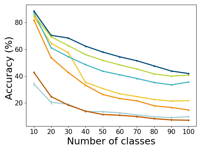
(a) $|{\mathcal{M}}|=300$

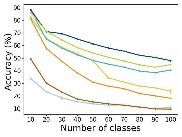
(b) $|{\mathcal{M}}|=500$

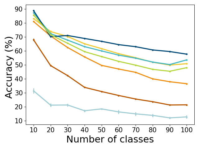
(c) $|{\mathcal{M}}|=2000$

Figure 2: Baseline CIL methods comparison on Split CIFAR-100 with different fixed buffer sizes. For each method, each point represents the average accuracy achieved on the corresponding task $t$, $A_{t}$.

Probably because the memory buffer is so small, and as can be seen in Fig. 2, GEM and GDumb perform poorly in a relative comparison. BiC performs well on buffer size 2000, but significantly degrades for smaller buffers for which it is not suited. iCarl demonstrates high performance, but it is highly non-modular, being heavily dependent on the Herding selection strategy while using a K-Means classifier. Hence we cannot integrate it with TEAL.

We are therefore left with methods XDER, ER-ACE and ER, which are both suitable and competitive, to be examined with and without TEAL as the selection mechanism. For ER-ACE, since it depends on populating the buffer with exemplars at the beginning of the task before training on the new classes, we cannot rely on the representation provided by a trained model. Therefore, we adjust the integration of TEAL by filling the buffer in two stages: First, at the beginning of task $t$, we update the buffer with exemplars from the new classes using the random-sampling selection strategy. Second, after training task $t$, we replace the exemplars from the new classes in the buffer with exemplars chosen using TEAL. It’s important to note that throughout this process, the buffer maintains the fixed size of exemplars it allowed, ensuring compliance with the class-incremental framework.

4.2 Main results

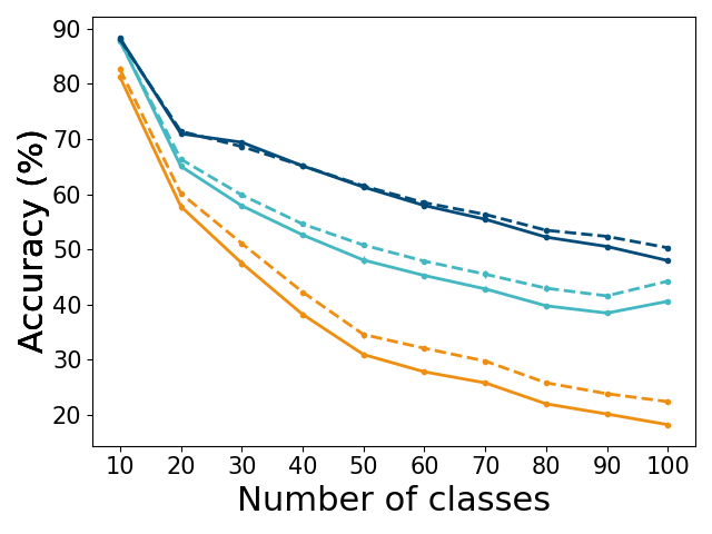
(b) $|{\mathcal{M}}|=500$

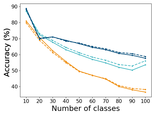
(c) $|{\mathcal{M}}|=2000$

Split CIFAR-100

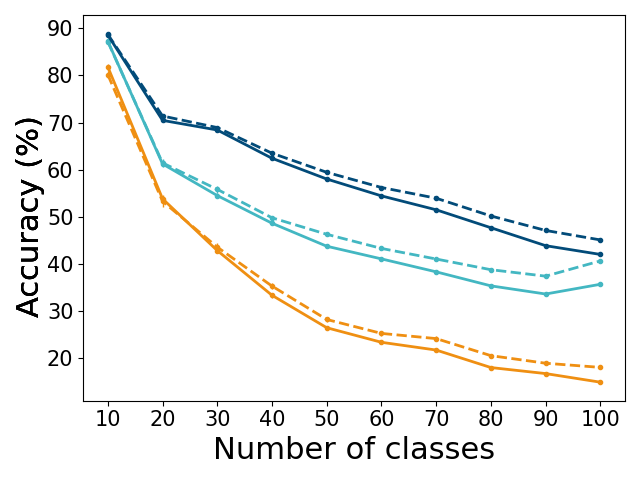
(a) $|{\mathcal{M}}|=300$

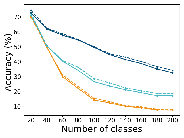
(e) $|{\mathcal{M}}|=1000$

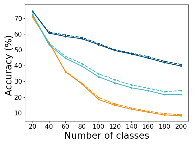
(f) $|{\mathcal{M}}|=2000$

Split tinyImageNet

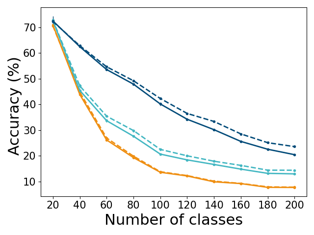
(d) $|{\mathcal{M}}|=400$

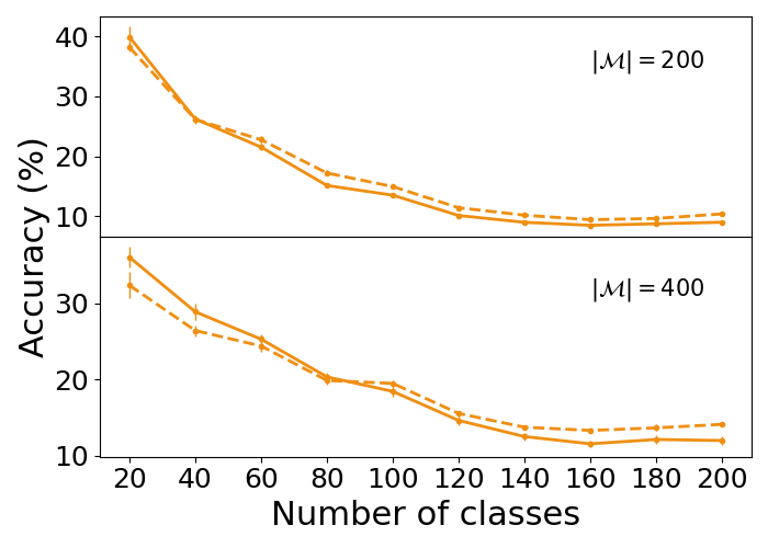
(h) ER

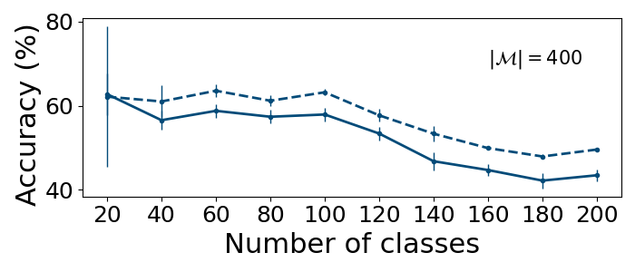
(i) XDER

Split CUB-200

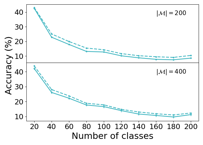
(g) ER-ACE

Figure 3: The performance of ER-IL methods with and without TEAL. Each plot displays the average accuracy after training incrementally on a different number of classes. Each color corresponds to a different ER-IL method, where the continuous line represents the vanilla method, while the dashed line represents the method with TEAL as its selection strategy. The error bars correspond to standard error based on 4-10 repetitions.

4.2.1 TEAL integrated with SOTA ER-IL methods

Split CIFAR-100

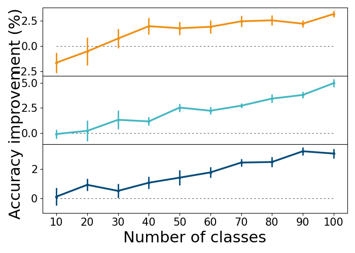
(a) $|{\mathcal{M}}|=300$

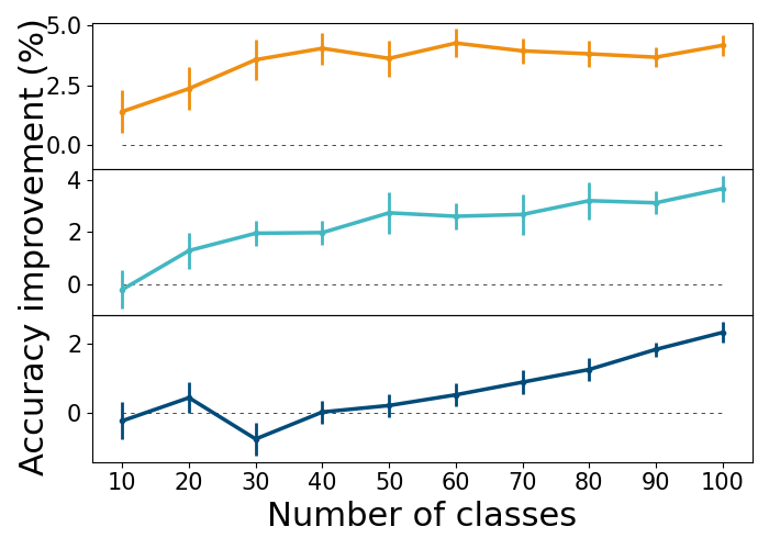
(b) $|{\mathcal{M}}|=500$

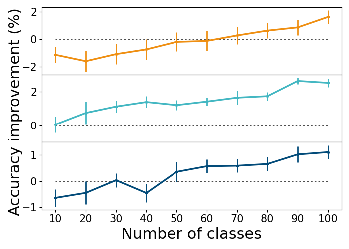
(c) $|{\mathcal{M}}|=2000$

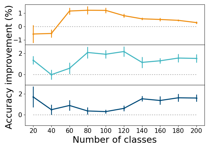
(e) $|{\mathcal{M}}|=1000$

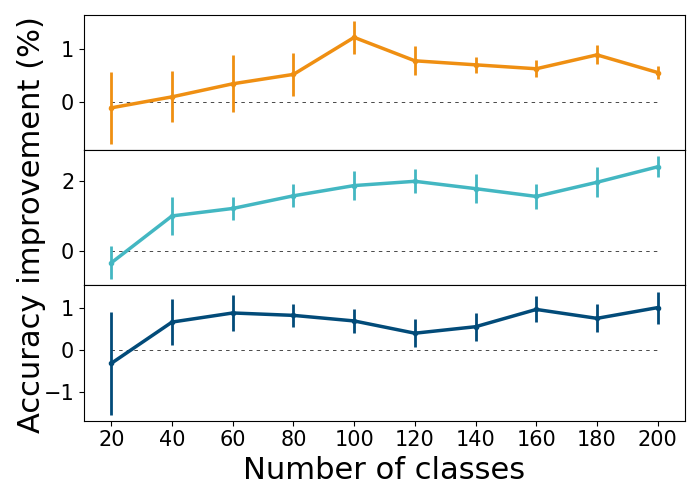
(f) $|{\mathcal{M}}|=2000$

Split tinyImageNet

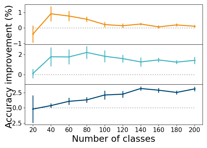
(d) $|{\mathcal{M}}|=400$

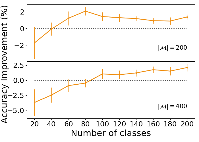
(h) ER

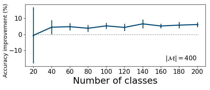
(i) XDER

Split CUB-200

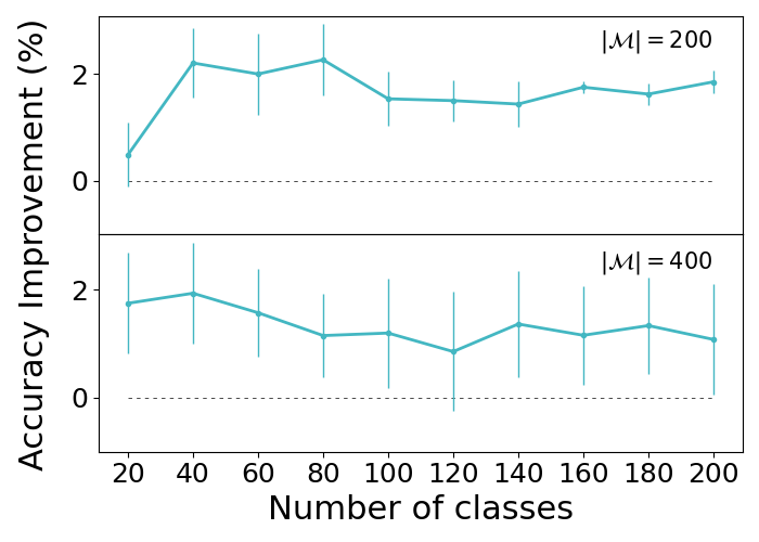
(g) ER-ACE

Figure 4: Performance improvement of TEAL when integrated with different ER-IL methods. Each graph depicts the difference in accuracy between TEAL and another method (XDER, ER-ACE, and ER) across all tasks. The first two rows present the three methods improvement on Split CIFAR-100 and Split tinyImageNet with different fixed buffer sizes denoted as $|{\mathcal{M}}|$. The last row pertains to Split CUB-200, where each graph showcases different buffer sizes for a different method.

Table 1: Final average accuracy for method with and without TEAL

Dataset	Split CIFAR-100			Split tinyImageNet			Split CUB-200
$|{\mathcal{M}}|$	300	500	2000	400	1000	2000	200	400
XDER	41.97±0.25	47.97±0.22	57.69±0.21	20.49±0.19	32.68±0.24	39.76±0.31	–	43.63±1.78
XDER+TEAL	45.05±0.24	50.29±0.2	58.79±0.17	23.61±0.32	34.28±0.24	40.76±0.23	–	49.55±0.47
Improvement	3.08	2.32	1.1	3.13	1.59	1.0	–	5.96
ER-ACE	35.63±0.36	40.6±0.34	53.6±0.17	13.02±0.2	17.37±0.34	21.71(±0.17)	8.56±0.15	11.25±0.99
ER-ACE+TEAL	40.59±0.2	44.25±0.35	56.11±0.19	14.43±0.29	18.88±0.21	24.12±0.24	10.41±0.16	12.33±0.26
Improvement	4.97	3.65	2.51	1.41	1.51	2.4	1.85	1.08
ER	14.82±0.21	18.21±0.29	36.54±0.31	7.75±0.06	7.7±0.06	8.27±0.08	8.98±0.18	12.01±0.52
ER+TEAL	17.97±0.25	22.39±0.31	38.17±0.37	7.86±0.05	7.99±0.06	8.82±0.09	10.37±0.23	14.13.76±0.3
Improvement	3.15	4.18	1.62	0.11	0.29	0.56	1.39	2.12

As mentioned above, we investigate the baseline methods XDER, ER-ACE and ER, comparing their performance when using either their native selection strategies or TEAL. We examined Split CIFAR-100 with buffer sizes of 300, 500 and 2000, Split tinyImageNet with buffer sizes of 400, 1000 and 2000, and Split CUB-200 with buffer sizes of 200 and 400. Fig. 3 shows the average accuracy $A_{t}$ after each task $t$. Fig. 4 shows the corresponding improvement of TEAL. Finally, the results of the final average accuracy $A_{t}$ and the differences ’improved-vanilla’ are reported in Table 1.

As demonstrated in Fig. 4, in most cases, the improvement achieved by TEAL increases as incremental training progresses, resulting in a more significant improvement by the final task. Indeed, we do not expect significant differences immediately after the first task, as catastrophic forgetting hasn’t occurred yet. Reassuringly, for the majority of the experiments, the improvement becomes apparent starting from the second task.

Table 1 shows that the difference (’improvement’ row) is always positive, namely, TEAL always improves the outcome. Looking at the improvement row for the XDER method, it is evident that the improvement provided by TEAL increases as the buffer size decreases. This trend is also demonstrated for ER-ACE and partially for ER on Split CIFAR-100.

4.2.2 Comparison of selection strategy

We begin with a simple ER-IL model on Split CIFAR-100 with various buffer sizes, and three different selection strategies: random, Herding and TEAL. As depicted in Fig. 5, our method enhances performance as compared to random selection by almost 3% for smaller buffers (300, 400, 500) and about 2.5% for larger buffers (1000, 2000). When compared to Herding, our method is more effective for smaller buffer sizes, enhancing performance by up to 1.2% for a buffer size of 300, but less effective with large buffers. Similar results, using different class ordering, are shown in App A.1.

Figure 5: Split CIFAR-100: performance difference between TEAL and either random-sampling or Herding selection. Each bar corresponds to a fixed buffer size.

Dataset	Split CIFAR-100
$|{\mathcal{M}}|$	300	500	2000
XDER+TEAL_OneTime	44.13±0.26	49.87±0.22	59.05±0.14
XDER+TEAL	45.05±0.24	50.29±0.2	58.79±0.17
ER-ACE+TEAL_OneTime	35.81±0.42	40.16±0.3	51.52±0.24
ER-ACE+TEAL	36.4±0.12	40.26±0.23	51.68±0.35
ER+TEAL_OneTime	17.64±0.12	22.01±0.18	40.65±0.32
ER+TEAL	18.1±0.1	22.07±0.13	39.96±0.23

Table 2: The improvement of 2 variants of TEAL when integrated with different CIL methods: XDER, ER-ACE and ER. In almost all cases, the original TEAL matches or outperforms the OneTime variant.

Given the results shown in Fig. 5, wherein TEAL seems less effective than herding with large buffers when training the simple baseline model, we repeat this comparison while integrating both methods - TEAL and Herding - into competitive ER-IL methods. Fig. 6 shows the difference between the improvement obtained by TEAL and the one obtained by Herding. Since in almost all cases this difference is positive, we may conclude that TEAL is significantly more beneficial than Herding.

(a) $|{\mathcal{M}}|=300$

(b) $|{\mathcal{M}}|=500$

(c) $|{\mathcal{M}}|=2000$

Figure 6: The difference between the improvement obtained by TEAL and the one obtained by Herding, showing 2 ER-IL methods and 3 buffer sizes while training on the Split CIFAR-100 dataset.

4.3 Ablation study

We explore an alternative variant of TEAL, which selects the set of exemplars in a single pass. We call this variant TEAL_OneTime. While still selecting exemplars for each class separately, this variant first partitions the exemplars of each class into $n=\frac{|{\mathcal{M}}|}{N^{t}}$ clusters, and then selects the most typical exemplar from each cluster in descending order of cluster size, preserving the order of selections.

The experiments on the two variants are conducted using Split CIFAR-100 with the smaller version of ResNet-18 mentioned in Section 4.1 and buffer sizes of 300, 500 and 2000. We investigate the performance enhancement of each variant when integrated with XDER, ER-ACE, and ER. The results are shown in Table 2. Whenever there is a significant difference in performance, the iterative variant outperforms the other one in 4 out of 5 cases. However, the differences are not substantial.

5 Summary and discussion

We propose a new mechanism to select exemplars for the memory buffer in replay-based CIL methods. This method is based on the principles of diversity and representativeness. When the memory buffer is relatively small, our method TEAL is shown to outperform both the native mechanism of each ER-IL method (usually random selection) and an alternative selection mechanism called Herding. Even when the buffer is large, our method is beneficial in almost all studied cases.

Our future work will investigate ways to determine at which point, if any, the added value of our method diminishes or possibly becomes harmful. We will also integrate TEAL with other replay-based CIL methods that utilize different selection strategies, and analyze the impact on their performance.

Acknowledgement

This work was supported by grants from the Israeli Council of Higher Education and the Gatsby Charitable Foundations.

Appendix

Appendix A Implementation details

The source code used in this study would be uploaded to our GitHub repository and will be made public upon acceptance.

TEAL, as described in Alg. 1, requires an iterations pace $s_{1}\leq\dots\leq s_{k}=n$ which indicates the pace of selecting exemplars from new class data. In both settings we use a logarithmic pace. We set a base $b=1.4$, and define $s_{1}=\lfloor b^{4}\rfloor,s_{2}=\lfloor b^{5}\rfloor,\dots,s_{k}=\lfloor b^{log_{b}n}\rfloor$.

A.1 Stand-alone setting

For all selection strategies, we use a smaller ResNet-18, as mentioned above, trained for 200 epochs. Optimization is performed with an SGD optimizer using Nesterov momentum of 0.9, a weight decay of 0.0002, and a learning rate that starts at 0.1 and decays by a factor of 0.3 every 66 epochs. Training is conducted with a batch size of 128 examples, and data augmentation is applied through random cropping and horizontal flips.

We run this setting on Split CIFAR-100 with three different random orders of classes:

1. The Order we display on Fig. 5 is: [44, 19, 93, 90, 71, 69, 37, 95, 53, 91, 81, 42, 80, 85, 74, 56, 76, 63, 82, 40, 26, 92, 57, 10, 16, 66, 89, 41, 97, 8, 31, 24, 35, 30, 65, 7, 98, 23, 20, 29, 78, 61, 94, 15, 4, 52, 59, 5, 54, 46, 3, 28, 2, 70, 6, 60, 49, 68, 55, 72, 79, 77, 45, 1, 32, 34, 11, 0, 22, 12, 87, 50, 25, 47, 36, 96, 9, 83, 62, 84, 18, 17, 75, 67, 13, 48, 39, 21, 64, 88, 38, 27, 14, 73, 33, 58, 86, 43, 99, 51]

2. The order in 7(a) is: [45, 15, 90, 32, 35, 63, 17, 72, 79, 96, 48, 36, 16, 11, 23, 80, 22, 58, 3, 62, 50, 33, 66, 99, 43, 76, 7, 57, 81, 82, 6, 10, 24, 52, 95, 73, 91, 21, 38, 31, 85, 59, 13, 69, 75, 70, 64, 8, 77, 34, 46, 39, 92, 0, 44, 98, 49, 9, 4, 61, 12, 83, 28, 78, 40, 88, 54, 5, 26, 41, 89, 20, 84, 2, 1, 55, 19, 74, 25, 37, 42, 14, 30, 18, 67, 71, 68, 27, 60, 51, 29, 56, 93, 47, 97, 94, 86, 87, 65, 53]

3. The order in 7(b) is: [48, 97, 1, 81, 90, 49, 10, 8, 7, 20, 70, 73, 75, 14, 91, 38, 47, 21, 74, 52, 80, 98, 59, 12, 71, 85, 6, 34, 55, 82, 95, 63, 78, 15, 94, 60, 99, 76, 25, 40, 88, 0, 62, 96, 87, 51, 16, 18, 9, 19, 29, 45, 86, 53, 56, 31, 28, 61, 30, 33, 4, 67, 64, 58, 50, 54, 3, 13, 37, 27, 66, 77, 84, 69, 2, 41, 22, 92, 42, 44, 11, 36, 46, 79, 65, 72, 23, 17, 39, 5, 89, 35, 24, 83, 43, 57, 93, 32, 68, 26]

(a) Order 2

(b) Order 3

Figure 7: Enhanced accuracy of TEAL compared to random-sampling and Herding selection strategies, additional two different classes order.

A.2 Integrated setting

Here we train a ResNet-18 model for 100 epochs using the same optimizer as in A.1, with the same batch size and data augmentations, with some exceptions. ER-ACE starts with a learning rate of 0.01, and all experiments on Split CUB-200 are conducted for 30 epochs with a batch size of 16 due to the dataset size and the resolution of its images.

A.3 Baselines setting

The setting for the experiments of the baseline methods is the same as in A.2 with some exceptions. For BiC, the number of training epochs is 250, and the learning rate scheduler decays the learning rate by a factor of 0.1 on epochs 100, 150 and 200. For GEM, the batch size is 32 and the learning rate starts from 0.03.For GDumb, the batch size is 32. For iCaRL the learning rate starts from 2, the weight decay is 0.00001 and the learning rate scheduler decays the learning rate by a factor of 0.2 on epochs 49 and 63.

Appendix B Compute resources

All experiments involved training deep learning models, necessitating the use of GPUs. For the Split CIFAR-100 experiments, 10 GB of GPU memory was used. The Split tinyImageNet experiments required 22 GB of GPU memory, while the Split CUB-200 experiments utilized 45 GB of GPU memory. Any other experiments conducted for the full research and not reported in the paper required the same compute resources.

References

- Boschini et al. [2022] Matteo Boschini, Lorenzo Bonicelli, Pietro Buzzega, Angelo Porrello, and Simone Calderara. Class-incremental continual learning into the extended der-verse. IEEE transactions on pattern analysis and machine intelligence, 45(5):5497–5512, 2022.
- Caccia et al. [2021] Lucas Caccia, Rahaf Aljundi, Nader Asadi, Tinne Tuytelaars, Joelle Pineau, and Eugene Belilovsky. New insights on reducing abrupt representation change in online continual learning. arXiv preprint arXiv:2104.05025, 2021.
- Chaudhry et al. [2018] Arslan Chaudhry, Marc’Aurelio Ranzato, Marcus Rohrbach, and Mohamed Elhoseiny. Efficient lifelong learning with A-GEM. CoRR, abs/1812.00420, 2018. URL http://arxiv.org/abs/1812.00420.
- Chaudhry et al. [2019a] Arslan Chaudhry, Marcus Rohrbach, Mohamed Elhoseiny, Thalaiyasingam Ajanthan, P Dokania, P Torr, and M Ranzato. Continual learning with tiny episodic memories. In Workshop on Multi-Task and Lifelong Reinforcement Learning, 2019a.
- Chaudhry et al. [2019b] Arslan Chaudhry, Marcus Rohrbach, Mohamed Elhoseiny, Thalaiyasingam Ajanthan, Puneet Kumar Dokania, Philip H. S. Torr, and Marc’Aurelio Ranzato. Continual learning with tiny episodic memories. CoRR, abs/1902.10486, 2019b. URL http://arxiv.org/abs/1902.10486.
- Choi et al. [2021] Yoojin Choi, Mostafa El-Khamy, and Jungwon Lee. Dual-teacher class-incremental learning with data-free generative replay. In Proceedings of the IEEE/CVF Conference on Computer Vision and Pattern Recognition, pages 3543–3552, 2021.
- De Lange et al. [2021] Matthias De Lange, Rahaf Aljundi, Marc Masana, Sarah Parisot, Xu Jia, Aleš Leonardis, Gregory Slabaugh, and Tinne Tuytelaars. A continual learning survey: Defying forgetting in classification tasks. IEEE transactions on pattern analysis and machine intelligence, 44(7):3366–3385, 2021.
- Gao and Liu [2023] Rui Gao and Weiwei Liu. Ddgr: Continual learning with deep diffusion-based generative replay. In International Conference on Machine Learning, pages 10744–10763. PMLR, 2023.
- Gautam et al. [2024] Chandan Gautam, Sethupathy Parameswaran, Ashish Mishra, and Suresh Sundaram. Generative replay-based continual zero-shot learning. In Towards Human Brain Inspired Lifelong Learning, pages 73–100. World Scientific, 2024.
- Hacohen et al. [2022] Guy Hacohen, Avihu Dekel, and Daphna Weinshall. Active learning on a budget: Opposite strategies suit high and low budgets. In International Conference on Machine Learning. PMLR, 2022.
- He et al. [2016] Kaiming He, Xiangyu Zhang, Shaoqing Ren, and Jian Sun. Deep residual learning for image recognition. In 2016 IEEE Conference on Computer Vision and Pattern Recognition, CVPR 2016, Las Vegas, NV, USA, June 27-30, 2016, pages 770–778. IEEE Computer Society, 2016. doi: 10.1109/CVPR.2016.90. URL https://doi.org/10.1109/CVPR.2016.90.
- Hou et al. [2019] Saihui Hou, Xinyu Pan, Chen Change Loy, Zilei Wang, and Dahua Lin. Learning a unified classifier incrementally via rebalancing. In Proceedings of the IEEE/CVF conference on computer vision and pattern recognition, pages 831–839, 2019.
- Krizhevsky et al. [2009] Alex Krizhevsky, Geoffrey Hinton, et al. Learning multiple layers of features from tiny images. Online, 2009.
- Le and Yang [2015] Ya Le and Xuan S. Yang. Tiny imagenet visual recognition challenge. 2015. URL https://api.semanticscholar.org/CorpusID:16664790.
- Li and Hoiem [2017] Zhizhong Li and Derek Hoiem. Learning without forgetting. IEEE transactions on pattern analysis and machine intelligence, 40(12):2935–2947, 2017.
- Lomonaco et al. [2021] Vincenzo Lomonaco, Lorenzo Pellegrini, Andrea Cossu, Antonio Carta, Gabriele Graffieti, Tyler L Hayes, Matthias De Lange, Marc Masana, Jary Pomponi, Gido M Van de Ven, et al. Avalanche: an end-to-end library for continual learning. In Proceedings of the IEEE/CVF Conference on Computer Vision and Pattern Recognition, pages 3600–3610, 2021.
- Lopez-Paz and Ranzato [2017] David Lopez-Paz and Marc’Aurelio Ranzato. Gradient episodic memory for continual learning. Advances in neural information processing systems, 30, 2017.
- Mallya and Lazebnik [2018] Arun Mallya and Svetlana Lazebnik. Packnet: Adding multiple tasks to a single network by iterative pruning. In Proceedings of the IEEE conference on Computer Vision and Pattern Recognition, pages 7765–7773, 2018.
- Masana et al. [2022] Marc Masana, Xialei Liu, Bartłomiej Twardowski, Mikel Menta, Andrew D Bagdanov, and Joost Van De Weijer. Class-incremental learning: survey and performance evaluation on image classification. IEEE Transactions on Pattern Analysis and Machine Intelligence, 45(5):5513–5533, 2022.
- McCloskey and Cohen [1989] Michael McCloskey and Neal J Cohen. Catastrophic interference in connectionist networks: The sequential learning problem. In Psychology of learning and motivation, volume 24, pages 109–165. Elsevier, 1989.
- Prabhu et al. [2020] Ameya Prabhu, Philip HS Torr, and Puneet K Dokania. Gdumb: A simple approach that questions our progress in continual learning. In Computer Vision–ECCV 2020: 16th European Conference, Glasgow, UK, August 23–28, 2020, Proceedings, Part II 16, pages 524–540. Springer, 2020.
- Rebuffi et al. [2017] Sylvestre-Alvise Rebuffi, Alexander Kolesnikov, Georg Sperl, and Christoph H Lampert. icarl: Incremental classifier and representation learning. In Proceedings of the IEEE conference on Computer Vision and Pattern Recognition, pages 2001–2010, 2017.
- Shin et al. [2017] Hanul Shin, Jung Kwon Lee, Jaehong Kim, and Jiwon Kim. Continual learning with deep generative replay. Advances in neural information processing systems, 30, 2017.
- Tian et al. [2024] Songsong Tian, Lusi Li, Weijun Li, Hang Ran, Xin Ning, and Prayag Tiwari. A survey on few-shot class-incremental learning. Neural Networks, 169:307–324, 2024.
- Van de Ven et al. [2022] Gido M Van de Ven, Tinne Tuytelaars, and Andreas S Tolias. Three types of incremental learning. Nature Machine Intelligence, 4(12):1185–1197, 2022.
- Wah et al. [2011] Catherine Wah, Steve Branson, Peter Welinder, Pietro Perona, and Serge Belongie. The caltech-ucsd birds-200-2011 dataset. 2011.
- Welling [2009] Max Welling. Herding dynamical weights to learn. In Proceedings of the 26th annual international conference on machine learning, pages 1121–1128, 2009.
- Wu et al. [2019] Yue Wu, Yinpeng Chen, Lijuan Wang, Yuancheng Ye, Zicheng Liu, Yandong Guo, and Yun Fu. Large scale incremental learning. In Proceedings of the IEEE/CVF conference on computer vision and pattern recognition, pages 374–382, 2019.