RTGS: Enabling Real-Time Gaussian Splatting on Mobile Devices Using Efficiency-Guided Pruning and Foveated Rendering

Abstract.

Point-Based Neural Rendering (PBNR), i.e., the 3D Gaussian Splatting-family algorithms, emerges as a promising class of rendering techniques, which are permeating all aspects of society, driven by a growing demand for real-time, photorealistic rendering in AR/VR and digital twins. Achieving real-time PBNR on mobile devices is challenging.

This paper proposes RTGS, a PBNR system that for the first time delivers real-time neural rendering on mobile devices while maintaining human visual quality. RTGS combines two techniques. First, we present an efficiency-aware pruning technique to optimize rendering speed. Second, we introduce a Foveated Rendering (FR) method for PBNR, leveraging humans’ low visual acuity in peripheral regions to relax rendering quality and improve rendering speed. Our system executes in real-time (above 100 FPS) on Nvidia Jetson Xavier board without sacrificing subjective visual quality, as confirmed by a user study. The code is open-sourced at https://github.com/horizon-research/Fov-3DGS.

1. Introduction

Rendering technologies are infiltrating every facet of society. For instance, rendering is critical to enabling digital twins (juarez2021digital, ) in emerging areas such as smart cities, digital healthcare, and telepresence. Reinvigorated interests in Augmented/Virtual Reality (AR/VR) further heighten the demand for real-time, photorealistic rendering.

Point-Based Neural Rendering (PBNR), i.e., the Gaussian Splatting-family algorithms (Kerbl2023GaussianSplatting, ; fan2023lightgaussian, ; lee2024compact, ; fang2024mini, ; niemeyer2024radsplat, ; girish2023eagles, ), emerges as a new class of rendering solutions, which revitalizes the classic point-based rendering techniques (gross2011point, ; levoy1985use, ; pfister2000surfels, ; zwicker2001surface, ) using modern neural rendering methods (mildenhall2021nerf, ). PBNR, like previous neural rendering algorithms such as Neural Radiance Fields (NeRF), offers photorealistic rendering by learning light-matter interactions from data, but is significantly faster by replacing the compute-intensive Multilayer Perceptrons (MLPs) in NeRF with lightweight point-based rasterization.

Nevertheless, PBNR is still far from real-time on mobile devices, rendering generally below 10 Frames-Per-Second (FPS) on the mobile Volta GPU (xaviersoc, ). This paper introduces RTGS, which, for the first time, delivers real-time PBNR on mobile devices while maintaining human visual quality. RTGS combines two key ingredients.

Efficiency-Aware Pruning.

Much of the recent efforts on optimizing PBNR models focus on pruning (fan2023lightgaussian, ; lee2024compact, ; fang2024mini, ; niemeyer2024radsplat, ; girish2023eagles, ), which, while reducing the model size, does not bring significant speedups. This is because existing pruning methods are single-minded in reducing the sheer number of points while being agnostic to the actual computational cost. We find that different points in a PBNR model contribute differently to the overall computation. Instead, we propose an efficiency-aware pruning method that directly optimizes for the rendering/inference speed (Sec. 3).

Foveated PBNR.

RTGS also exploits characteristics of human vision to improve performance (Sec. 4). Human vision acuity is poor in the visual periphery (wandell1995foundations, ), an opportunity that has long been exploited: one can speed up rendering by gradually reducing the rendering quality as the pixel eccentricity increases (i.e., as pixels are positioned more at the visual periphery) with impunity, a technique known as Foveated Rendering (FR) (patney2016towards, ; guenter2012foveated, ).

We introduce the first FR method for PBNR. We gradually reduce the number of points used for rendering as the pixel eccentricity increases. The key is a data representation, where points at higher eccentricies are purposely designed to be a strict subset of the points at lower eccentricies. That way, (most of the) parameters and computation are shared when rendering different eccentricity regions, improving performance and reducing storage requirements.

Equally important to improving performance is to maintain a high visual quality. To that end, we introduce a new training method, which guides both pruning and peripheral quality relaxation (in FR) by explicitly modeling human visual perception at different eccentricies. As a result, the subjective visual quality is consistent across the visual field and is aligned with the dense, non-FR model.

Result.

We evaluate our method using both subjective human studies and objective measurements of performance and quality. Across 12 participants, the subjective rendering quality of our method is statistically no worse than that of Mini-Splatting-D  (fang2024mini, ), the PBNR method that is the current best in rendering quality. Compared to five state-of-the-art PBNR methods, we outperform all of them in both objective rendering quality (by up to 0.4 dB in PSNR) and rendering speed (by up to 7.4$\times$ on a mobile Volta GPU).

The contributions of this paper are as follows:

• We propose an efficiency-aware pruning method for PBNR that directly targets computational efficiency rather than merely reducing point counts.

• We propose the first FR method tailored for PBNR; the method is centered around a new data/point representation, which improves rendering performance with little storage overhead.

• We introduce a training framework that incorporates both pruning and FR while maintaining subjective visual quality; the key is to explicitly model HVS and use the model to guide training.

2. Background

We first introduce the necessary background in PBNR (Sec. 2.1), followed by the main characteristics of the Human Visual System (HVS) and how they are used by Foveated Rendering to improve rendering speed (Sec. 2.2).

Fig. 1. Illustration of PBNR, which parameterizes the scene with a set of points, each associated with a 3D Gaussian distribution that gives rise to an ellipsoid. The ellipsoids are projected to ellipses on the image plane, where the ellipses are sorted (per tile, e.g., $2\times 2$ pixels). The color of a pixel is calculated by integrating the contribution of each intersecting ellipse (e.g., a, c, d, e for p).

2.1. Point-Based Neural Rendering

PBNR is a class of neural rendering techniques, exemplified by the 3D Gaussian Splatting (3DGS) algorithm (Kerbl2023GaussianSplatting, ) and its descendants (fan2023lightgaussian, ; lee2024compact, ; fang2024mini, ; niemeyer2024radsplat, ; girish2023eagles, ). Compared to previous neural rendering techniques, a.k.a., the NeRF-family algorithms (mildenhall2021nerf, ; barron2022mip, ; muller2022instant, ; chen2022tensorf, ; sun2022direct, ), PBNR is fundamentally more efficient (e.g., usually over 1,000 times faster), because it parameterizes the scene with discrete points (rather than voxels) to avoid redundant computations and renders via a lightweight rasterization-based process called splatting (rusinkiewicz2000qsplat, ; zwicker2001surface, ; ren2002object, ) rather than the heavy MLP inference.

General PBNR Pipeline.

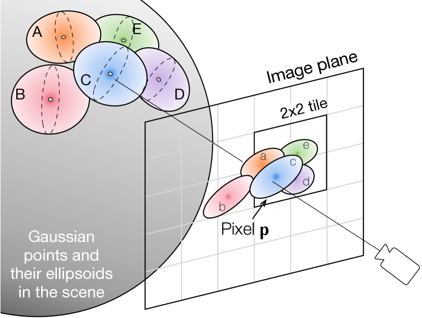
We use 3DGS as a running example to explain the general pipeline of PBNR, which all PBNR algorithms follow. Fig. 1 illustrates the general idea. Rendering starts with an offline-trained model, which contains a set of discrete points (A–E) that represent the scene. Each point is associated with an ellipsoid, whose three-dimensional scales are determined by the $\sigma$s of a 3D Gaussian distributions (hence the name Gaussian point). Each ellipsoid has a set of trainable parameters, including the scales, position, orientation, opacity, color distribution (which is parameterized through Spherical Harmonics; SH).

Given the trained points/ellipsoids, the online rendering follows three steps: Projection, Sorting, and Rasterization.

Projection.  Each ellipsoid is first projected/splatted to an ellipse on the image plane. In the example of Fig. 1, the ellipsoids A–E in the scene are splatted to ellipses a–e on the image plane. The goal is to identify, for each pixel tile (e.g., $2\times 2$), which ellipses intersect with the tile and thus contribute to the pixel colors in the tile.

Sorting.  For each tile, we sort all the intersecting ellipses based on their depths to the image plane; that way, closer ellipses can be weighted more when calculating pixel colors. For instance in Fig. 1, ellipse c would be the closest.

Rasterization.  Finally, we calculate the intersections of all the ellipses in a tile with each pixel. The color of a pixel p is then computed using the classic volume rendering method (max1995volume_rendering, ; kaufman1993volume, ; levoy1988display, ), which integrates the contribution of all the intersecting ellipses from near to far:

(1a) $$\textbf{p}=\sum_{i=0}^{N-1}T_{i}\alpha_{i}c_{i},~{}~{}~{}T_{i}=\prod_{j=0}^{i-1}(1-\alpha_{j})$$

(1b) $$\alpha_{i}=f(\text{opacity}_{i},...,\text{pose})$$

(1c) $$c_{i}=g(\text{SH}_{0},...,\text{SH}_{n})$$

where $N$ is the number of ellipses intersecting p (i.e., a, c, d, e in Fig. 1), $\alpha_{i}$ is a function $f$ of various trainable parameters of the $i^{th}$ intersecting ellipse (e.g., opacity) and the camera pose, and $c_{i}$ is the color of the $i^{th}$ ellipse at the position of intersection, which is calculated using the Spherical Harmonics (SH) function $g$ with trainable coefficients $\text{SH}_{n}$. We refer readers to Kerbl et al. (Kerbl2023GaussianSplatting, ) for the details of $f$ and $g$.

2.2. Human Visual System and Foveated Rendering

Foveated Rendering.

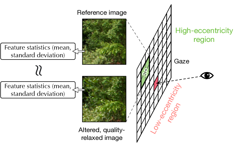
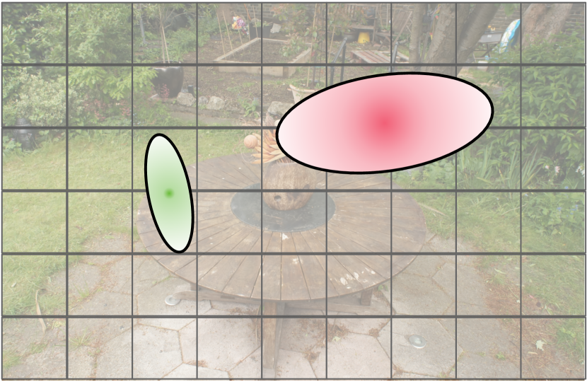
It is well-known that human visual acuity drops as eccentricity increases, i.e., when objects are placed more toward the visual periphery (wandell1995foundations, ). This is due to a combination of larger pooling sizes (rodieck1985parasol, ; dacey1993mosaic, ) and a sparser photoreceptor distribution (curcio1990human, ; Song:2011:ConeDensity, ) on the retina as the eccentricity increases. Foveated Rendering (FR) (patney2016towards, ; guenter2012foveated, ) leverages this natural fall-off in visual acuity to speed up rendering by relaxing the rendering quality in peripheral regions. Fig. 2 illustrates an example where the visual content in high-eccentricity regions could be altered without being noticeable by users.

While in classic FR the peripherial rendering quality is relaxed by lowering the resolution, neural rendering offers another dimension: reducing the computational workload of each pixel. This new dimension is possible because the rendering load of each pixel is controlled by inferencing a deep learning model, which offers many knobs for accuracy-vs-speed trade-offs that have been extensively studied (han2015learning, ; blalock2020state, ; jin2020adabits, ; yang2019quantization, ). For instance, one can train a smaller model for rendering the visual periphery (deng2022fov, ). This paper will explore FR knobs unique to PBNR.

Modeling HVS.

A key question in FR is to determine how much quality to relax without introducing visual artifacts. It is well-established that commonly used visual quality metrics such as Peak Signal to Noise Ratio (PSNR) or Structural Similarity Index Measure (SSIM) (hore2010image, ) do not account for the eccentricity-dependent visual acuity drop in HVS (walton2021beyond, ; rosenholtz2016capabilities, ; strasburger2011peripheral, ) and, thus, are inadequate for FR: an image with a low PSNR at the visual periphery might not introduce visual artifacts. The altered image in Fig. 2, when placed in the visual periphery, is visually indiscriminable from the reference image.

This paper leverages an eccentricity-aware HVS Quality (HVSQ) metric (walton2021beyond, ) inspired by classic neuroscience studies about the human visual pathway (FreemanSimoncelli2011, ). Given a reference image, an altered image, and the eccentricity of each pixel (which depends on the display resolution and the eye-display distance), HVSQ quantifies how similar the two images are as viewed by humans; a lower HVSQ means more similar.

The principle behind the HVSQ metric is as follows. The retina aggregates photoreceptor outputs in spatial regions, called spatial poolings. In the image space, a spatial pooling corresponds to a set of adjacent pixels (e.g., SP in Fig. 2). The pooling size increases with eccentricity, usually quadratically. Computational models on HVS (walton2021beyond, ) show that as long as the statistics (mean and standard deviation) of the content in a spatial pooling between two images are close, humans can not discriminate between them. The statistics are calculated in a feature space (as opposed to the pixel space) to emulate the feature extraction in human’s early visual processing.

Computationally, the HVSQ of an altered image with respect to a reference image is calculated as follows:

(2) $$HVSQ=\frac{1}{N}\sum_{i=1}^{N}\Big{[}\big{(}\mathcal{M}(\text{I}^{a}_{i})-\mathcal{M}(\text{I}^{r}_{i})\big{)}^{2}+\big{(}\sigma(\text{I}^{a}_{i})-\sigma(\text{I}^{r}_{i})\big{)}^{2}\Big{]}$$

where $N$ is the number of pixels in an image (each pixel has a unique spatial pooling), $\text{I}^{r}_{i}$ and $\text{I}^{a}_{i}$ denote the features of the $i^{th}$ spatial pooling in the reference and the altered image, respectively; $\mathcal{M}$ denotes arithmetic mean, and $\sigma$ denotes standard deviation.

Intuitively, the HVSQ metric calculates the average distance between the two images’ statistics across all the spatial poolings. HVSQ makes intuitive sense: as pixel eccentricities increase, the pooling sizes increase, which gives us more “wiggle room” within a spatial pooling to manipulate pixel values to match the feature statistics of the reference image.

Fig. 2. Pixels under the user’s gaze have low eccentricities, where the human visual quality is the highest; the peripheral pixels have high eccentricities where human visual acuity is low. In peripheral regions, the visual stimulus (image) can be altered without being discriminable from the reference stimulus if the statistics of the image features are close, as quantified by the HVSQ metric (Eqn. 2). SP: spatial pooling.

3. Efficiency-Aware Pruning

This section introduces a pruning framework to speed up PBNR. We first identify the root-cause why existing pruning methods are ineffective (Sec. 3.1). We then propose two techniques to address the root-cause: intersection-aware pruning (Sec. 3.2) and scale decay (Sec. 3.3). Finally, we discuss how these two techniques are combined together (Sec. 3.4).

Fig. 3. FPS distribution of recent PBNR models on common datasets measured on mobile Volta GPU on Jetson Xavier.

Fig. 4. Point count vs. latency per frame and the number of tile-ellipse intersections vs. latency per frame.

Fig. 5. Two ellipses intersect different number of tiles so contribute to computation cost differently.

3.1. Motivations

Speed.

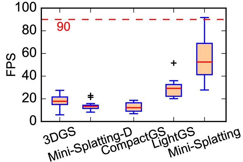
The performance of recent PBNR models is far from real-time on mobile GPUs. Fig. 5 shows the FPS on the Mip-NeRF 360 (barron2022mip, ), Tanks&Temples (Knapitsch2017, ), and Deep Belending (hedman2018deep, ) dataset, measured on the mobile Volta GPU on Jetson Xavier across five recent PBNR models (fan2023lightgaussian, ; lee2024compact, ; fang2024mini, ; Kerbl2023GaussianSplatting, ). The data is plotted as a standard boxplot to show the FPS distribution across the 13 traces within the datasets.

3DGS (Kerbl2023GaussianSplatting, ) and Mini-Splatting-D (fang2024mini, ) are two dense models and generally are the slowest. Much of recent work focuses on pruning: reducing the number of points in a PBNR model (fan2023lightgaussian, ; lee2024compact, ; fang2024mini, ). While effective for reducing the model size, these methods do not significantly speed up rendering. The last three models in Fig. 5 are pruned models. While generally faster, they are still far below real-time, especially for immersive applications such as AR/VR, which would normally require an FPS of 75–90 (vive_pro2, ; meta_quest_pro, ; apple_vision_pro, ).

Why is Existing Pruning Ineffective?

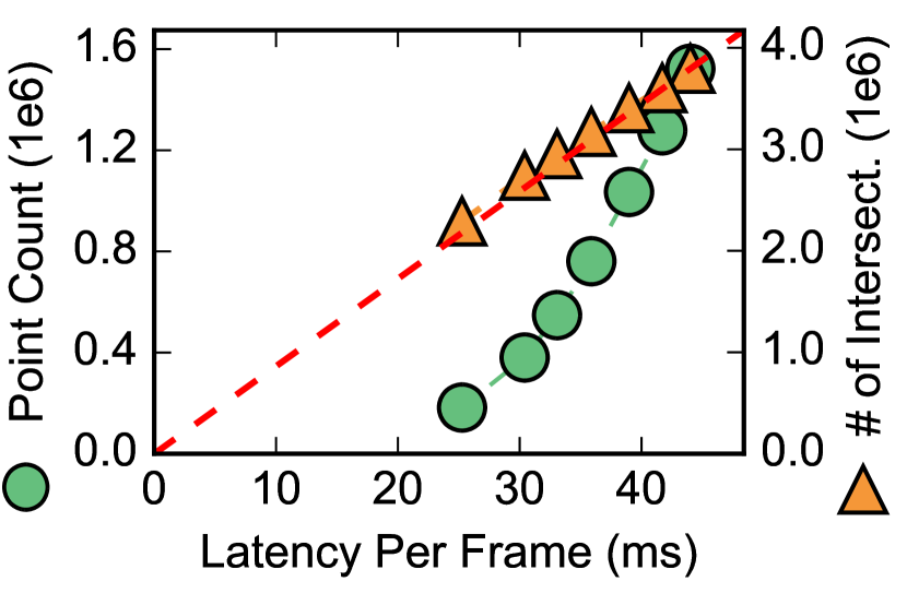
Existing pruning methods focus on reducing the point count in a model, which is ineffective for improving speed in PBNR. To quantify this, Fig. 5 shows the inference latency ($x$-axis) vs. point count (left $y$-axis) of LightGS (fan2023lightgaussian, ) (which prunes 3DGS (Kerbl2023GaussianSplatting, )) trained on the bicycle trace in the Mip-NeRF 360 dataset at different pruning levels (between 75% and 97%). The latency reduction rate is slower than that of the point reduction rate.

The reason that reducing the point count is ineffective for acceleration is because the computational costs associated with different points vary. Fig. 5 shows the intuition, where there are two ellipses projected onto the image plane. The smaller ellipse intersects with only two tiles whereas the larger one intersects with eight. As a result, the larger one is used in calculating more pixel colors and is naturally responsible for more computation.

Therefore, what does impact the inference speed is the number of tile-ellipse intersections. Fig. 5 shows the latency vs. the average number of intersections per tile (right $y$-axis) for each pruned LightGS model; the latency reduction rate and intersection reduction rate match.

3.2. Intersection-Aware Pruning

The goal of our pruning is to judiciously reduce tile-ellipse intersections without affecting the visual quality. The key to our pruning is a metric that we call Computational Efficiency (CE), which intuitively describes how much contribution a point makes to pixel values per unit cost of compute. Intuitively, we would like to prioritize pruning points with low CEs, as they consume a lot of computation without making much contribution to pixel values. For every point $i$ in a dense model, its CE is defined as:

(3) $$\text{CE}_{i}=\frac{\text{Val}_{i}}{\text{Comp}_{i}}$$

$\text{Val}_{i}$, contribution of a point $i$ to pixel values, is defined as the number of pixels that are “dominated” by that point. A pixel is dominated by a point if and only if that point, among all the points, has the highest numerical contribution to the pixel value during rasterization (Sec. 2.1). The numerical contribution of a point $i$ is quantified by $T_{i}\alpha_{i}$ in Eqn. 1a.

$\text{Comp}_{i}$, the compute cost of a point $i$, which is ignored in all existing pruning methods, is quantified by the number of tiles that intersect and use (the ellipse of) that point, which directly affects the rendering speed as established above.

In actual rendering, a point will be used in different frames based on the camera pose. Thus, a point’s CE is frame-specific; in extreme cases, a point could be outside the camera’s viewing frustum and thus makes no contribution to the image. We empirically find that the final CE of a point is adequately measured by the maximum CE across all poses (as opposed to the average, which is susceptible to dataset bias) in the training set.

With this metric, during pruning we sort all the points by their CEs and remove a certain portion of points with the lowest CEs. How many points to remove must be done in conjunction with controlling the quality of the pruned model, which we will discuss in Sec. 3.4.

3.3. Scale Decay

Orthogonal to pruning points, another way to reduce tile-ellipse intersections is to reduce the ellipse size/scale, which we call “scale decay.” In particular, we want to focus on scaling ellipses that are both large and are used by a lot of tiles in rendering. To guide scale decay, we propose a metric called Weighted Scale (WS) that weighs the point sizes with how often they are used in rendering:

(4) $$\text{WS}=\frac{1}{N}\sum\limits_{i=0}^{N-1}\text{S}_{i}\text{G}_{i}$$

where $N$ is the number of points, $\text{S}_{i}$ is the scale of point $i$’s ellipse (the maximum span of the ellipse in any direction). Without $\text{G}_{i}$, WS is simply the average scale of all points in a model. $\text{G}_{i}$ weighs a point’s scale by how often it is used in rendering, and is defined as:

(5) $$\text{G}_{i}=(\text{U}_{i}>T)\cdot(\text{U}_{i}-T)$$

where $\text{U}_{i}$ is the number of tiles a point $i$ is used in rendering and $T$ is a threshold; intuitively, if a point $i$ is used by fewer than $T$ tiles, its scale is insignificant, in which case the $\text{G}_{i}$ is 0 so $i$ does not participate in calculating the average scale. That way, the G term helps suppressing the scale of points that are not only large but are also used often in rendering.

The WS metric is a general metric characterizing point/ellipse scales in PBNR. We empirically find that it is particularly effective when integrated into the training process as an additional term to the loss function $\mathcal{L}$, which ordinarily is concerned only with the rendering quality ($\mathcal{L}_{\text{quality}}$):

(6) $$\mathcal{L}=\mathcal{L}_{\text{quality}}+\gamma\cdot\text{WS}$$

where $\gamma$ is a hyper-parameter governing how much scale decay to apply.

3.4. Putting It Together

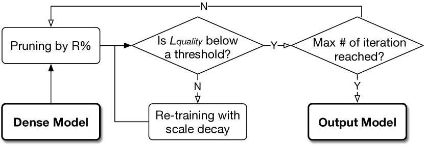
Pruning and scale decay are conceptually orthogonal, but, importantly, scaling an ellipse’s size also changes its CE. Thus, scale decay must be done in conjunction with pruning. Fig. 6 illustrates the general procedure.

Given a dense model, we first compute the CE for all the points, and repetitively prune a small percentage ($R=10\%$ in our implementation) of the points with the lowest CEs until the quality loss ($\mathcal{L}_{\text{quality}}$ in Eqn. 6) is above a prescribed threshold. We then train the pruned model again to regain the quality, but using the composite loss $\mathcal{L}$ in Eqn. 6 in order to apply scale decay. The re-training continues until $\mathcal{L}_{\text{quality}}$ is once again below the threshold, at which point we apply intersection-aware pruning again. We iteratively apply pruning and scale decay in such a way until a certain number of iterations is reached.

Note that $\mathcal{L}_{\text{quality}}$ is usually PSNR or SSIM but can be any other quality metric of interest. In the next section we will show how we can use a human vision-inspired quality metric to account for the eccentricity dependence of visual quality.

Our iterative procedure has two advantages. First, it combines pruning and scale decay. Second, it does not require quality-specific hyper-parameter tuning to achieve a specific visual quality: monitoring and controlling for $\mathcal{L}_{quality}$ automatically yield a model at a given quality.

4. Foveated PBNR

Fig. 6. The procedure to obtain an efficient PBNR model given a dense model. We iteratively apply pruning and re-training with scale decay (guided by $\mathcal{L}$ in Eqn. 6) while controlling for quality ($\mathcal{L}_{quality}$).

Fig. 7. The general idea of FR for PBNR. : We train multiple models (four in this example), each with a different quality and is responsible for rendering a different quality region in the image ($$R1$$ – $$R4$$). The four quality regions are blended together to generate the final image. The goal is for the FR-rendered image to have the same visual quality as the reference image (e.g., generated by a dense model) when judged by humans. : Points in the original non-FR model. : Our hierarchical point representation to support compute- and data-efficient FR. We subset the points so that points used to train a higher-level (lower quality) model are strictly a subset of that used by a lower-level model. The quality bound $m$ of a point is the highest level that uses the point (e.g., $m=3$ for Point 4). : To provide more flexibility for training, we selectively allow key trainable parameters to differ across levels; these parameters are the opacity of a point and the Direct Current (DC) component of the SH coefficients ($\text{SH}_{\text{DC}}$). Other (trainable) parameters of a point are shared across all the levels that use the point (e.g., no parameter in $L_{4}$ for Point 4). : The rendering pipeline augmented to support FR (augmentations in green).

This section introduces a Foveated Rendering (FR) method tailored to PBNR. We first describe the main idea and its main challenges (Sec. 4.1). We then discuss an efficient data representation that enables effective FR for PBNR (Sec. 4.2). Finally, we describe how to train FR models leveraging the efficiency-aware pruning discussed before (Sec. 4.3).

4.1. Main Idea and Challenges

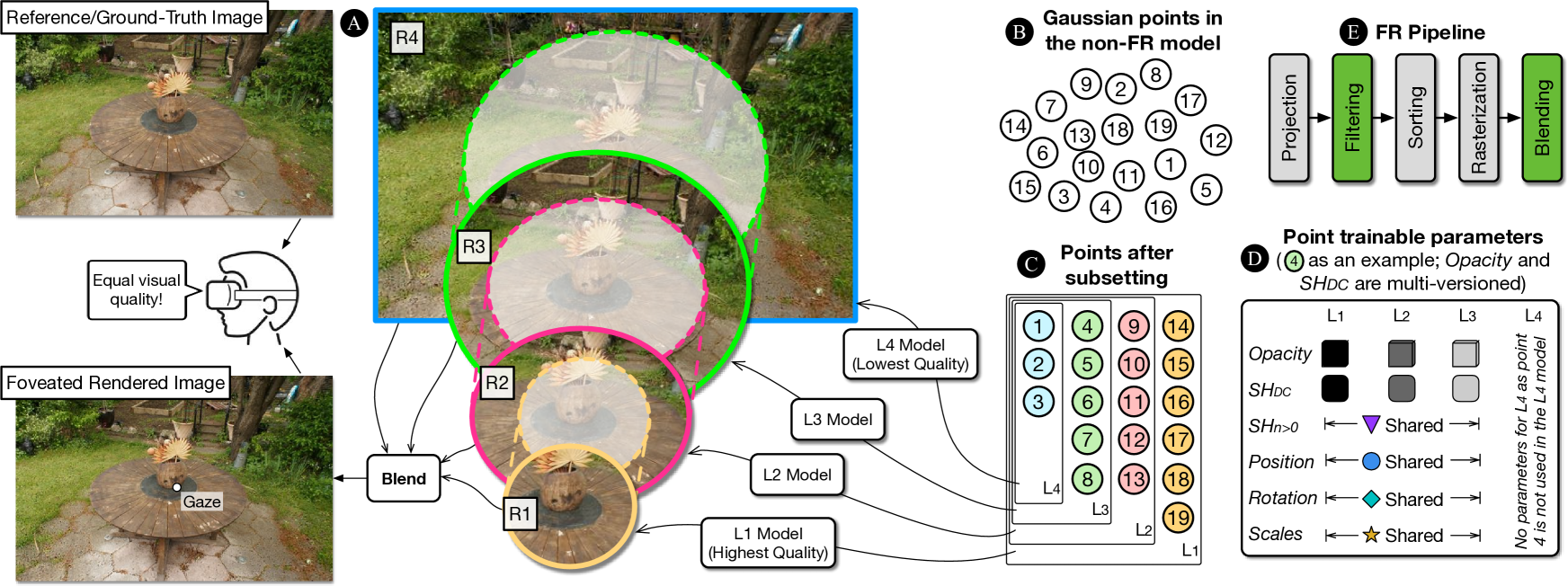
We accelerate rendering by relaxing the rendering quality at the visual periphery, leveraging the low peripheral visual acuity in HVS. We illustrate the idea in Fig. 7, panel .

Main Pipeline.

As with prior FR work (deng2022fov, ; guenter2012foveated, ; patney2016towards, ), we divide an image into $N$ regions (4 in the example), each corresponding to a quality level and is rendered by a separate model. The region currently under the user’s gaze has the highest quality ($$R1$$ here). Lower-quality regions are rendered using lighter models, which are obtained by applying pruning and scale decay (Sec. 3) to a high-quality model.

Panel shows the rendering pipeline augmented to support FR — with two new stages (green). First, after projection we must filter each model’s points that are outside the model’s quality region. Second, after each region is rendered, we must blend the results together to avoid aliasing.

Blending is required in all FR algorithms (guenter2012foveated, ; patney2016towards, ). Due to the quality difference across levels, there is a sharp, undesirable boundary between two adjacent levels in the rendered image (a form of aliasing). To eliminate the boundary, a common technique is for each model to render slightly beyond its assigned boundary; thus, pixels at the boundary will be rendered twice and then are interpolated/blended to provide a smooth transition between the two levels.

While this multi-model FR idea is conceptually simple, we must address three challenges.

Challenge 1: Performance Overhead.

FR can potentially accelerate rendering because it reduces the amount of rasterization work in low-quality regions. However, it has two sources of performance overhead.

First, all $N$ models must go through the Projection and Filtering stages. In our profiling, these two stages can take up to 18% of the rendering time. Second, blending also adds overhead. Empirically we find that about 25% of the pixels are to be blended and, thus, rendered twice.

Challenge 2: Storage Overhead.

FR could increase the model size due to the need to store multiple models, exacerbating the storage pressure of PBNR models. For instance, the bicycle scene in the Mip-NeRF 360 dataset (barron2021mip, ) takes about 1.4 GB of space when trained with 3DGS (Kerbl2023GaussianSplatting, ); recent pruning methods  (fan2023lightgaussian, ) reduce the model size of that scene to about 490 MB, which is still large for mobile devices.

We address the first two challenges using an efficient data representation, as we will discuss in Sec. 4.2.

Challenge 3: Controlling Quality.

FR must be done in a way that guarantees human visual quality — how do we decide the amount of relaxation at each level? We describe a training strategy to guarantee consistent human visual quality across all levels, as described in Sec. 4.3.

4.2. Efficient Data Representation

To address both the performance and storage overhead, we propose an efficient data representation that allows models at different quality levels to share computation and parameters. The key idea is that points used to train and render a lower quality level are strictly a subset of the points used by a higher quality level. Panel in Fig. 7 illustrates how the original points in Panel are organized after subsetting. Level 1 ($L_{1}$) model is trained with the most points and thus would offer the highest quality, and Level 4 ($L_{4}$) model has the fewest points and lowest quality.

Subsetting mitigates both the performance and storage overhead, because the total number of points across all $N$ models, $P_{total}$, is the same as that of the highest-quality model, $P_{1}$, rather than the sum of all $N$ models. That is, $P_{total}=\text{max}_{i=1}^{N}{P_{i}}=P_{1}<\sum_{i=1}^{N}{P_{i}}$. As a result, there is no storage overhead. The compute overhead is small too, since the Projection and Filtering stages are executed only once, rather than once for each of the $N$ models.

Under subsetting, each point is simultaneously used in models $[L_{1},\cdots,L_{m}]$, where $m$ is the highest level beyond which the point is not used and is called the quality bound of the point. For instance in Fig. 7, $m=3$ for Points 4. During the Projection stage, each point is projected to a tile, which has a specific eccentricity and thus a corresponding quality level $t$. If $t>m$, the point does not participate in the rest of rendering. This is the Filtering stage in Panel .

Selective Multi-Versioning.

Practically, strict subsetting is likely too restrictive in controlling the rendering quality at different levels. This is because all the trainable parameters of a point would be fixed across all levels, so how a point participates in calculating pixel colors (the $\alpha_{i}c_{i}$ term in Eqn. 1a) is also fixed at any time. In reality, however, a point’s contribution to pixel colors should vary depending on the quality region the point is projected to, which varies with the camera pose and the gaze position.

To relax this, we allow multi-versioning as illustrated in panel : a point can maintain $m$ (where $m$ is the quality bound of the point) versions of some of its trainable parameters, one version for each level the point is in. Empirically, we allow four such parameters, i.e., the Opacity and the Direct Current component of the SH coefficients ($\text{SH}_{DC}$); these four parameters are empirically found to impact the pixel colors the most. We will show in Sec. 6.3 that selective multi-versioning is critical to maintain high visual quality.

4.3. HVS-Guided Training

The discussion so far has focused on performance, but equally important to FR is the visual quality: how much weaker can higher-level models be while maintaining subjectively good visual quality across quality levels/eccentricies?

To answer this question, we turn to the HVSQ metric discussed in Sec. 2.2. The HVSQ metric quantifies the subjective visual quality between a reference image (e.g., rendered from a dense PBNR model) and an altered image (e.g., rendered from a pruned PBNR model), accounting for the eccentricity-dependent visual acuity of HVS. Conveniently, while the vanilla HVSQ metric in Eqn. 2 is applied to an entire image, it can be easily adapted to a selected region — by simply iterating over the spatial poolings (pixels) in the selected region rather than over the entire image.

That way, each quality region has a unique HVSQ measure, and our goal is to ensure the HVSQs across all quality levels are similar to the HVSQ of the baseline model. To that end, we first train the highest-quality, $L_{1}$ model, which itself can be pruned and scale-decayed from a dense model. We then prune a $L_{1}$ model to obtain a $L_{2}$ model, which is pruned down to obtain a $L_{3}$ model; this continues until the desired level is achieved. The way to obtain a $L_{i+1}$ model follows the exact procedure as laid out in Sec. 3.4 (i.e., iteratively apply pruning and re-training to a $L_{i}$ model while controlling for the quality loss $\mathcal{L}_{quality}$) — with two key differences.

First, instead of using the usual PSNR/SSIM metrics, we use HVSQ as $\mathcal{L}_{quality}$ in Eqn. 6. In particular, when obtaining a $L_{i}$ model we use the HVSQ corresponding to level $i$. We control for $\mathcal{L}_{quality}$ so that the HVSQ at all quality levels is the same as that of $L_{1}$ such that the human visual quality is consistent across the entire visual field. Second, during iterative re-training we do not apply scale decay, because an ellipse scale is not part of the multi-versioned parameters.

5. Experimental Setup

FR Training Procedure.

We use four quality regions whose eccentricity starts at 0°, 18°, 27°, and 33°, respectively, corresponding to about 13%, 17%, 21%, 49% of image pixels in these four regions, respectively.

We use Mini-Splatting-D (fang2024mini, ), the current-best in quality, as the baseline dense PBNR model. The $L_{1}$ model is obtained from the dense model through pruning and scale decay as described in Sec. 3.4, with an iteration budget of 50,000, followed by another 5,000 iterations of fine-tuning with HVSQ loss. The three lower-quality models are obtained from their immediately higher-quality model as described in Sec. 4.3, with a 7,500 iteration budget.

Variants.

We design three variants of our method, namely RTGS-H, RTGS-M, and RTGS-L, with decreasing rendering quality. The $L_{1}$ model in the three variants is pruned to have a PSNR of 99%, 98%, and 97% of that of the dense model. The total model size of the three variants is 16%, 12%, and 10%, respectively, of that of the dense model.

Datasets.

We evaluate three real-world datasets: Mip-Nerf360 (barron2022mip, ), Tanks & Temple (Knapitsch2017, ), and DeepBlending (hedman2018deep, ), which amounts to 13 traces in total. The camera poses in the datasets are usually very sparsely populated, which is not representative of the continuous rendering scenario (e.g., VR). We interpolate between the poses in the dataset to create smooth trajectories, producing approximately 1,440 poses for each trace, corresponding to a 16-second video at 90 FPS.

Baselines.

We compare against five recent PBNR models:

• Dense PBNR models: 3DGS (Kerbl2023GaussianSplatting, ), which is the earliest PBNR model, and Mini-Splatting-D (fang2024mini, ), which produce the state-of-the-art rendering quality.

• Pruned PBNR models: LightGS (fan2023lightgaussian, ), CompactGS (lee2024compact, ), Mini-Splatting (fang2024mini, ). The first two are pruned from 3DGS and the last one is from Mini-Splatting-D.

We also compare with two FR methods applied to PBNR. Both methods use the same quality-region division as in our method. The first one is SMFR (Single-Model FR), which uses a single dense PBNR model, which is the $L_{1}$ model in RTGS-H, and randomly samples the points when rendering lower-quality regions. It is effectively a strict subsetting version of our model without selective multi-versioning. The second one is MMFR (Multi-Model FR) (deng2022fov, ), whose $L_{1}$ model is the same as that of RTGS-H and whose higher-level models are pruned from its $L_{1}$ model separately (without subsetting). The number of points used in each level in both methods matches that used in our method.

User Study Procedure.

To assess the subjective rendering quality of our method, we perform a user study; the procedure is approved by our Internal Review Board (IRB). We recruited 12 participants (8 males and 4 females between 20 and 30 years old), all with normal or corrected-to-normal vision. We select four scenes from the three datasets: bicycle, room, drjohnson, and truck, which vary in both content and complexity. We then render the scenes using our RTGS-H and Mini-Splatting-D, which, recall, is the current-best in rendering quality.

Since Mini-Splatting-D does not render in real-time on a mobile device, we use a workstation with an RTX 4090 GPU to execute both models, both of which render smoothly at 90 FPS. The workstation streams, in real-time, the rendering to a Meta Quest Pro headset, which has an eye tracker to track the user’s real-time gaze.

We use the classic Two-Interval Forced Choice (2IFC) procedure (perez2019pairwise, ; chen2024pea, ), which is commonly used in psychophysics to compare the quality of two videos. For each trace, we display its rendering by the two methods on the headset in a random order to each participant, with a 5-second rest interval in-between. Each participant is then asked to pick which of the two versions they prefer. Each trace is repeated eight times, and the repetitions across traces are also randomized. The entire experiment lasts about one hour for each participant.

6. Evaluation

Fig. 8. The average number of times the two methods are preferred by users (a tie would be 4-vs-4). Error bars indicate the standard deviation within the participants. Users either have no preference or prefer our method (binomial test on the average result; $p$ ¡ 0.01).

Fig. 9. Performance and objective rendering quality (PSNR) comparison across the five baselines and the three RTGS variants on the mobile Volta GPU. 3DGS and Mini-Splatting-D are dense models, and the other three baselines are pruned models.

Fig. 10. Ablation study teasing apart the impact of various techniques. The FPS results are obtained on Jetson Xavier and averaged over all traces.

6.1. Subjective Experiments.

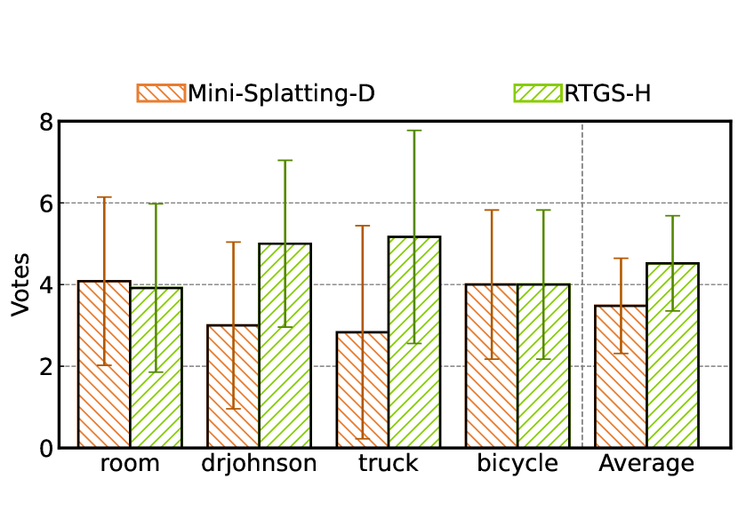
Fig. 10 shows the average number of participants who prefer the two methods for each video. A tie would be 4-vs-4, since each video is watched eight times by each user. We find that users either have no preference or prefer our method over Mini-Splatting-D. The results are statistically significant through a binomial test with $p$ ¡ 0.01; the null hypothesis is “users prefer Mini-Splatting-D more than 50% of the time”.

It might initially look surprising that we have equal or better subjective quality than Mini-Splatting-D, a dense model from which we prune and build our FR model. Further inspection and interviewing participants show two reasons. First, our HVS-aware fine-tuning (Sec. 5) better aligns the statistics of human-sensitive features with the ground truth. Second, some points in the dense model are trained with inconsistent information across camera poses, leading to incorrect luminance changes over time; pruning those points helps alleviate this inconsistency.

6.2. Mobile GPU Results

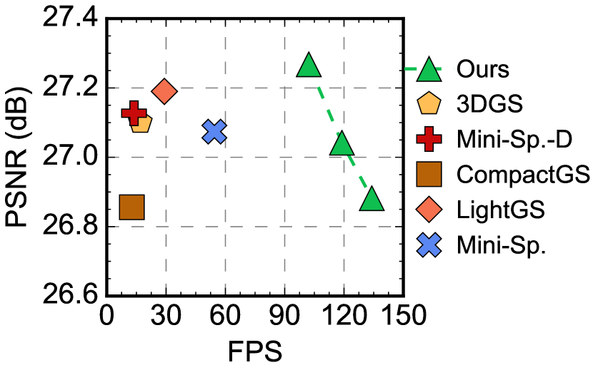
We now show the performance results on the mobile Volta GPU on Nvidia Jetson AGX Xavier (xaviersoc, ), a representative mobile device for use-cases such as VR. Fig. 10 shows the results. We execute each model five times for each camera pose in each scene in all the datasets, and report the average FPS.

To put the performance results in context, we also compare the PSNR metric of our variants with the baselines. PSNR is a good objective quality measure of the region under the user’s gaze and is universally reported in prior work. Using an objective metric also allows us to scale up the study to more traces. The SSIM results are similar and omitted.

Our three variants Pareto-dominate the baselines. Our slowest variant RTGS-H is 1.9$\times$ faster than the fastest baseline while being 0.1 dB higher than the best-quality baseline. The fastest variant RTGS-L is 7.9$\times$ faster than 3DGS, and can be up to 19.8$\times$ on the largest bicycle trace.

Ablation Studies.

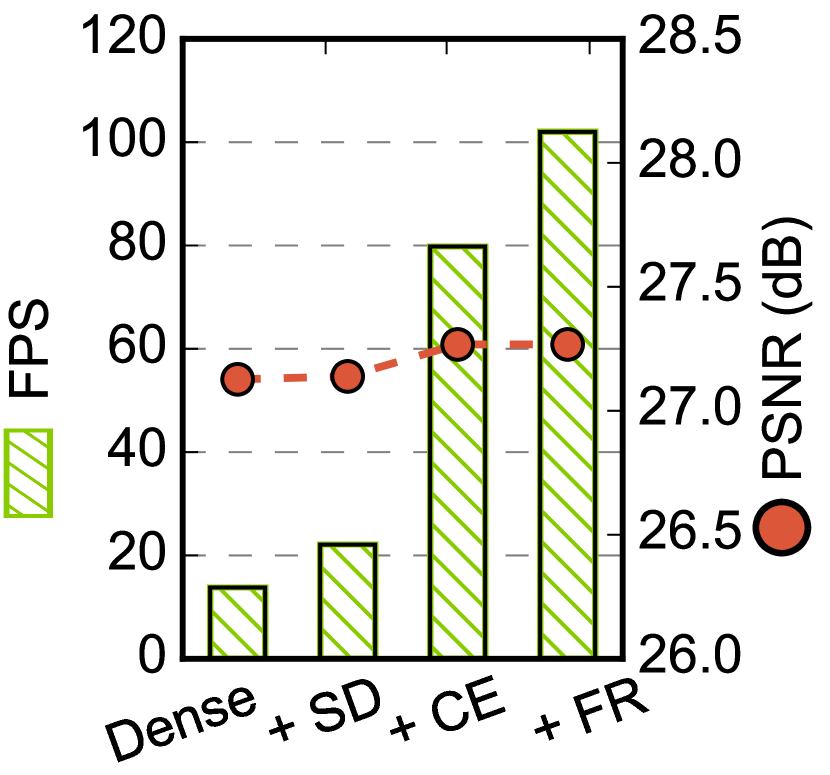
We now ablate the contribution of various performance-enhancing techniques. Fig. 10 shows the FPS (left $y$-axis) and PSNR (right $y$-axis) under: 1) the dense Mini-Splatting-D model, 2) RTGS with only scale decay (SD; Sec. 3.3), 3) RTGS with SD and CE-based pruning (Sec. 3.2), and 4) RTGS with SD, CE, and FR (Sec. 4). We use the RTGS-H model and obtain the FPS/PSNR results on Xavier averaged over all traces.

The PSNRs for all the variants are similar. With a similar quality, our SD implementation achieves 1.6$\times$ speedup compared to original dense model; CE-based pruning and FR bring the speedup to 5.8$\times$ and 7.4$\times$, respectively. CE reduces the model size by 85%, and FR diminishes the pruning rate only marginally to 84% owing to selective multi-versioning,.

Table 1. Comparison of FR methods.

Methods	FPS $\uparrow$	Storage (MB) $\downarrow$	HVS Quality ($\times 10^{-5}$)$\downarrow$
			L1	L2	L3	L4
SMFR	125.9 (1$\times$)	161.6 (1$\times$)	2.12	10.1	21.7	28.3
MMFR	52.6 (0.42$\times$)	311.0 (1.92 $\times$)	2.12	1.87	1.79	1.76
RTGS-H	102.2 (0.81$\times$)	171.8 (1.06$\times$)	2.12	2.10	2.09	2.08

6.3. Comparison with Other FR Methods

RTGS also out-performs the two FR baselines. Tbl. 1 compares the FPS (on the mobile Volta GPU), storage requirement, and the HVSQ metric across different quality regions/layers. The results are averaged across all the datasets.

SMFR has been seen as a variant of our FR with strict subsetting (no multi-versioning). Thus, it is the fastest, but has excessively low visual quality, because it simply sub-samples pre-trained points to render low-quality regions. Its HVSQ in $L_{4}$ is over 10$\times$ worse than the other two methods. Users confirm that subjectively this gives the worst quality.

Our method selectively multi-versioned four trainable parameters out of about 60 (Sec. 4.2 and in Fig. 7), so the additional storage requirement is small (about 6%). Note that RTGS-H already reduces the dense model size to 16% as shown in Sec. 5.

MMFR can be seen as a variant of our FR that multi-versions all parameters. It is thus the slowest of the three — its FPS is way below a 90 FPS real-time requirement, and has the largest storage requirement. This is due to the compute and storage overhead discussed in Sec. 4.1. Its HVSQ metrics in higher levels (lower-quality regions) are better than that of ours. Given that our method is already subjectively no-worse than even a dense model (Sec. 6.1), this suggests that MMFR unnecessarily optimizes for details that are imperceptible to users, which we confirm with users.

7. Related Work

Foveated Rendering.

The graphics community has long exploited FR for real-time rendering (patney2016towards, ; guenter2012foveated, ; Chen2022InstantReality, ; Konrad2020GazeContingent, ; Kaplanyan2019Deepfovea, ; Krajancich2020Optimizing, ; Chakravarthula2021GazeContingent, ; Sun2017PerceptuallyGuided, ). Particularly relevant to our work, researchers have started applying FR to neural rendering (deng2022fov, ; rolff2023vrs, ; rolff2023interactive, ), such as Fov-NeRF (deng2022fov, ). Our work differs from them in two key ways. First, these methods exclusively focus on NeRF, whereas we focus on PBNR, which is shown to be fundamentally more efficient that NeRF. Second, some (deng2022fov, ) use the multi-model approach, similar to our MMFR baseline, which we out-perform (Sec. 6.3). Our FR method uses subsetting with selectively multi-versioning, addressing the performance overhead of evaluating multiple models (Sec. 4.1).

While conventional FR uses heuristics (e.g., blurring) to guide quality relaxation, recently researchers have investigated more principled ways to model human perception for quality relaxation (FreemanSimoncelli2011, ; walton2021beyond, ). This work leverages such theoretical work and integrates it into the training framework to demonstrate its practical utility.

Prior work has also leveraged eccentricity-dependent color perception of HVS to reduce display power and improve framebuffer compresison in VR (duinkharjav2022color, ; ujjainkar2024exploiting, ; chen2023imperceptible, ; chen2024pea, ), which is orthogonal to this work. A number of early VR video streaming frameworks assume that a user’s gaze is always at the center of the display and reduces the streaming resolution of peripheral regions to save bandwidth. We refer interested readers to EVR (leng2019energy, ) for one such example, which also includes a summary of work in that area.

Efficient PBNR.

Almost all existing work optimizing PBNR focuses on pruning, based on the observation that a considerable amount of points can be pruned without impacting the rendering quality. They usually do so by, e.g., explicitly training a mask to remove points (lee2024compact, ) or sorting points by their numerical contribution to pixel colors followed by removing low-contributing points (fan2023lightgaussian, ; girish2023eagles, ; niemeyer2024radsplat, ; fang2024mini, ). People have also investigated non-pruning methods, such as vector quantization (fan2023lightgaussian, ) and distillation (lee2024compact, ) techniques, to compress PBNR models.

Our work differs from them in two key ways. First, we show that point count is not indicative of performance; tile intersections are (Sec. 3.1). We propose an intersection-aware metric to guide pruning (Sec. 3.2). Second, we show an orthogonal technique, scale decay, that complements pruning (Sec. 3.3) and can be performed in conjunction with pruning to further achieve improve performance (Sec. 3.4).

8. Conclusions

We achieve over an order of magnitude speedup over existing PBNR models with no subjective quality loss through a user study. The speedup comes from: 1) a pruning techniques that directly optimizes for the compute-cost of PBNR, 2) FR specialized for PBNR. For the first time, we achieve real-time (100+ FPS) PBNR on mobile devices.

References

- [1] Apple vision pro specifications. https://www.apple.com/apple-vision-pro/specs/. Accessed: 2024-06-24.
- [2] Meta quest pro specifications. https://vr-compare.com/headset/metaquestpro. Accessed: 2024-06-24.
- [3] Nvidia reveals xavier soc details.
- [4] Vive pro 2 headset specifications. https://www.vive.com/us/product/vive-pro2/specs/.
- [5] Jonathan T Barron, Ben Mildenhall, Matthew Tancik, Peter Hedman, Ricardo Martin-Brualla, and Pratul P Srinivasan. Mip-nerf: A multiscale representation for anti-aliasing neural radiance fields. In Proceedings of the IEEE/CVF International Conference on Computer Vision, pages 5855–5864, 2021.
- [6] Jonathan T Barron, Ben Mildenhall, Dor Verbin, Pratul P Srinivasan, and Peter Hedman. Mip-nerf 360: Unbounded anti-aliased neural radiance fields. In Proceedings of the IEEE/CVF Conference on Computer Vision and Pattern Recognition, pages 5470–5479, 2022.
- [7] Davis Blalock, Jose Javier Gonzalez Ortiz, Jonathan Frankle, and John Guttag. What is the state of neural network pruning? Proceedings of machine learning and systems, 2:129–146, 2020.
- [8] P. Chakravarthula, Z. Zhang, O. Tursun, P. Didyk, Q. Sun, and H. Fuchs. Gaze-contingent retinal speckle suppression for perceptually-matched foveated holographic displays. IEEE Transactions on Visualization and Computer Graphics, 27(11):4194–4203, 2021.
- [9] Anpei Chen, Zexiang Xu, Andreas Geiger, Jingyi Yu, and Hao Su. Tensorf: Tensorial radiance fields. In European Conference on Computer Vision, pages 333–350. Springer, 2022.
- [10] K. Chen, T. Wan, N. Matsuda, A. Ninan, A. Chapiro, and Q. Sun. Pea-pods: Perceptual evaluation of algorithms for power optimization in xr displays. ACM Transactions on Graphics, 43(4):67, July 2024.
- [11] Kenneth Chen, Budmonde Duinkharjav, Nisarg Ujjainkar, Ethan Shahan, Abhishek Tyagi, Jiayi He, Yuhao Zhu, and Qi Sun. Imperceptible color modulation for power saving in vr/ar. In ACM SIGGRAPH 2023 Emerging Technologies, pages 1–2. 2023.
- [12] S. Chen, B. Duinkharjav, X. Sun, L.-Y. Wei, S. Petrangeli, J. Echevarria, C. Silva, and Q. Sun. Instant reality: Gaze-contingent perceptual optimization for 3d virtual reality streaming. IEEE Transactions on Visualization and Computer Graphics, 28(5):2157–2167, 2022.
- [13] Christine A Curcio, Kenneth R Sloan, Robert E Kalina, and Anita E Hendrickson. Human photoreceptor topography. Journal of comparative neurology, 292(4):497–523, 1990.
- [14] Dennis M Dacey. The mosaic of midget ganglion cells in the human retina. Journal of Neuroscience, 13(12):5334–5355, 1993.
- [15] Nianchen Deng, Zhenyi He, Jiannan Ye, Budmonde Duinkharjav, Praneeth Chakravarthula, Xubo Yang, and Qi Sun. Fov-nerf: Foveated neural radiance fields for virtual reality. IEEE Transactions on Visualization and Computer Graphics, 28(11):3854–3864, 2022.
- [16] Budmonde Duinkharjav, Kenneth Chen, Abhishek Tyagi, Jiayi He, Yuhao Zhu, and Qi Sun. Color-perception-guided display power reduction for virtual reality. ACM Transactions on Graphics (TOG), 41(6):1–16, 2022.
- [17] Zhiwen Fan, Kevin Wang, Kairun Wen, Zehao Zhu, Dejia Xu, and Zhangyang Wang. Lightgaussian: Unbounded 3d gaussian compression with 15x reduction and 200+ fps. arXiv preprint arXiv:2311.17245, 2023.
- [18] Guangchi Fang and Bing Wang. Mini-splatting: Representing scenes with a constrained number of gaussians. arXiv preprint arXiv:2403.14166, 2024.
- [19] Jeremy Freeman and Eero P. Simoncelli. Metamers of the ventral stream. Nature Neuroscience, 14(9):1195–1201, September 2011.
- [20] Sharath Girish, Kamal Gupta, and Abhinav Shrivastava. Eagles: Efficient accelerated 3d gaussians with lightweight encodings. arXiv preprint arXiv:2312.04564, 2023.
- [21] Markus Gross and Hanspeter Pfister. Point-based graphics. Elsevier, 2011.
- [22] Brian Guenter, Mark Finch, Steven Drucker, Desney Tan, and John Snyder. Foveated 3d graphics. ACM transactions on Graphics (tOG), 31(6):1–10, 2012.
- [23] Song Han, Jeff Pool, John Tran, and William Dally. Learning both weights and connections for efficient neural network. Advances in neural information processing systems, 28, 2015.
- [24] Peter Hedman, Julien Philip, True Price, Jan-Michael Frahm, George Drettakis, and Gabriel Brostow. Deep blending for free-viewpoint image-based rendering. ACM Transactions on Graphics (ToG), 37(6):1–15, 2018.
- [25] Alain Hore and Djemel Ziou. Image quality metrics: Psnr vs. ssim. In 2010 20th international conference on pattern recognition, pages 2366–2369. IEEE, 2010.
- [26] Qing Jin, Linjie Yang, and Zhenyu Liao. Adabits: Neural network quantization with adaptive bit-widths. In Proceedings of the IEEE/CVF Conference on Computer Vision and Pattern Recognition, pages 2146–2156, 2020.
- [27] Maria G. Juarez, Vicente J. Botti, and Adriana S. Giret. Digital Twins: Review and Challenges. Journal of Computing and Information Science in Engineering, 21:030802:1–030802:23, 2021.
- [28] A. S. Kaplanyan, A. Sochenov, T. Leimkühler, M. Okunev, T. Goodall, and G. Rufo. Deepfovea: Neural reconstruction for foveated rendering and video compression using learned statistics of natural videos. ACM Transactions on Graphics, 38(6), November 2019.
- [29] Arie Kaufman, Daniel Cohen, and Roni Yagel. Volume graphics. Computer, 26(7):51–64, 1993.
- [30] B. Kerbl, G. Kopanas, T. Leimkuehler, and G. Drettakis. 3d gaussian splatting for real-time radiance field rendering. ACM Transactions on Graphics, 42(4):1–14, August 2023.
- [31] Arno Knapitsch, Jaesik Park, Qian-Yi Zhou, and Vladlen Koltun. Tanks and temples: Benchmarking large-scale scene reconstruction. ACM Transactions on Graphics, 36(4), 2017.
- [32] R. Konrad, A. Angelopoulos, and G. Wetzstein. Gaze-contingent ocular parallax rendering for virtual reality. ACM Transactions on Graphics, 39, 2020.
- [33] B. Krajancich, P. Kellnhofer, and G. Wetzstein. Optimizing depth perception in virtual and augmented reality through gaze-contingent stereo rendering. ACM Transactions on Graphics, 39, 2020.
- [34] Joo Chan Lee, Daniel Rho, Xiangyu Sun, Jong Hwan Ko, and Eunbyung Park. Compact 3d gaussian representation for radiance field. In Proceedings of the IEEE/CVF Conference on Computer Vision and Pattern Recognition, pages 21719–21728, 2024.
- [35] Yue Leng, Chi-Chun Chen, Qiuyue Sun, Jian Huang, and Yuhao Zhu. Energy-efficient video processing for virtual reality. In Proceedings of the 46th International Symposium on Computer Architecture, pages 91–103, 2019.
- [36] Marc Levoy. Display of surfaces from volume data. IEEE Computer graphics and Applications, 8(3):29–37, 1988.
- [37] Marc Levoy and Turner Whitted. The use of points as a display primitive. 1985.
- [38] Nelson Max. Optical models for direct volume rendering. IEEE Transactions on Visualization and Computer Graphics, 1(2):99–108, 1995.
- [39] Ben Mildenhall, Pratul P Srinivasan, Matthew Tancik, Jonathan T Barron, Ravi Ramamoorthi, and Ren Ng. Nerf: Representing scenes as neural radiance fields for view synthesis. Communications of the ACM, 65(1):99–106, 2021.
- [40] Thomas Müller, Alex Evans, Christoph Schied, and Alexander Keller. Instant neural graphics primitives with a multiresolution hash encoding. ACM Transactions on Graphics (ToG), 41(4):1–15, 2022.
- [41] Michael Niemeyer, Fabian Manhardt, Marie-Julie Rakotosaona, Michael Oechsle, Daniel Duckworth, Rama Gosula, Keisuke Tateno, John Bates, Dominik Kaeser, and Federico Tombari. Radsplat: Radiance field-informed gaussian splatting for robust real-time rendering with 900+ fps. arXiv preprint arXiv:2403.13806, 2024.
- [42] Anjul Patney, Marco Salvi, Joohwan Kim, Anton Kaplanyan, Chris Wyman, Nir Benty, David Luebke, and Aaron Lefohn. Towards foveated rendering for gaze-tracked virtual reality. ACM Transactions on Graphics (TOG), 35(6):1–12, 2016.
- [43] Maria Perez-Ortiz, Aliaksei Mikhailiuk, Emin Zerman, Vedad Hulusic, Giuseppe Valenzise, and Rafał K Mantiuk. From pairwise comparisons and rating to a unified quality scale. IEEE Transactions on Image Processing, 29:1139–1151, 2019.
- [44] Hanspeter Pfister, Matthias Zwicker, Jeroen Van Baar, and Markus Gross. Surfels: Surface elements as rendering primitives. In Proceedings of the 27th annual conference on Computer graphics and interactive techniques, pages 335–342, 2000.
- [45] Liu Ren, Hanspeter Pfister, and Matthias Zwicker. Object space ewa surface splatting: A hardware accelerated approach to high quality point rendering. In Computer Graphics Forum, volume 21, pages 461–470. Wiley Online Library, 2002.
- [46] RW Rodieck, KF Binmoeller, and J Dineen. Parasol and midget ganglion cells of the human retina. Journal of Comparative Neurology, 233(1):115–132, 1985.
- [47] Tim Rolff, Ke Li, Julia Hertel, Susanne Schmidt, Simone Frintrop, and Frank Steinicke. Interactive vrs-nerf: Lightning fast neural radiance field rendering for virtual reality. In Proceedings of the 2023 ACM Symposium on Spatial User Interaction, pages 1–3, 2023.
- [48] Tim Rolff, Susanne Schmidt, Ke Li, Frank Steinicke, and Simone Frintrop. Vrs-nerf: Accelerating neural radiance field rendering with variable rate shading. In 2023 IEEE International Symposium on Mixed and Augmented Reality (ISMAR), pages 243–252. IEEE, 2023.
- [49] Ruth Rosenholtz. Capabilities and limitations of peripheral vision. Annual review of vision science, 2:437–457, 2016.
- [50] Szymon Rusinkiewicz and Marc Levoy. Qsplat: A multiresolution point rendering system for large meshes. In Proceedings of the 27th annual conference on Computer graphics and interactive techniques, pages 343–352, 2000.
- [51] Hongxin Song, Toco Yuen Ping Chui, Zhangyi Zhong, Ann E Elsner, and Stephen A Burns. Variation of cone photoreceptor packing density with retinal eccentricity and age. Investigative ophthalmology & visual science, 52(10):7376–7384, 2011.
- [52] Hans Strasburger, Ingo Rentschler, and Martin Jüttner. Peripheral vision and pattern recognition: A review. Journal of vision, 11(5):13–13, 2011.
- [53] Cheng Sun, Min Sun, and Hwann-Tzong Chen. Direct voxel grid optimization: Super-fast convergence for radiance fields reconstruction. In Proceedings of the IEEE/CVF Conference on Computer Vision and Pattern Recognition, pages 5459–5469, 2022.
- [54] Q. Sun, F.-C. Huang, J. Kim, L.-Y. Wei, D. Luebke, and A. Kaufman. Perceptually-guided foveation for light field displays. ACM Transactions on Graphics, 36(6), November 2017.
- [55] Nisarg Ujjainkar, Ethan Shahan, Kenneth Chen, Budmonde Duinkharjav, Qi Sun, and Yuhao Zhu. Exploiting human color discrimination for memory-and energy-efficient image encoding in virtual reality. In Proceedings of the 29th ACM International Conference on Architectural Support for Programming Languages and Operating Systems, Volume 1, pages 166–180, 2024.
- [56] David R Walton, Rafael Kuffner Dos Anjos, Sebastian Friston, David Swapp, Kaan Akşit, Anthony Steed, and Tobias Ritschel. Beyond blur: Real-time ventral metamers for foveated rendering. ACM Transactions on Graphics, 40(4):1–14, 2021.
- [57] Brian A Wandell. Foundations of vision. sinauer Associates, 1995.
- [58] Jiwei Yang, Xu Shen, Jun Xing, Xinmei Tian, Houqiang Li, Bing Deng, Jianqiang Huang, and Xian-sheng Hua. Quantization networks. In Proceedings of the IEEE/CVF conference on computer vision and pattern recognition, pages 7308–7316, 2019.
- [59] Matthias Zwicker, Hanspeter Pfister, Jeroen Van Baar, and Markus Gross. Surface splatting. In Proceedings of the 28th annual conference on Computer graphics and interactive techniques, pages 371–378, 2001.