Time Series Clustering with General State Space Models via Stochastic Variational Inference

Abstract

In this paper, we propose a novel method of model-based time series clustering with mixtures of general state space models (MSSMs). Each component of MSSMs is associated with each cluster. An advantage of the proposed method is that it enables the use of time series models appropriate to the specific time series. This not only improves clustering and prediction accuracy but also enhances the interpretability of the estimated parameters. The parameters of the MSSMs are estimated using stochastic variational inference, a subtype of variational inference. The proposed method estimates the latent variables of an arbitrary state space model by using neural networks with a normalizing flow as a variational estimator. The number of clusters can be estimated using the Bayesian information criterion. In addition, to prevent MSSMs from converging to the local optimum, we propose several optimization tricks, including an additional penalty term called entropy annealing. Experiments on simulated datasets show that the proposed method is effective for clustering, parameter estimation, and estimating the number of clusters.

[1]organization=Data Science and AI Innovation Research Promotion Center, addressline=Shiga University, country=Japan

[2]organization=Department of Data Science, addressline=Shiga University, country=Japan

1 Introduction

Time series data analyses have been conducted in various fields, including science, engineering, business, finance, economics, medicine, and politics [1, 2]. Time series clustering is an analysis method used to classify multiple time series data into groups with identical patterns. This technique is crucial for work in various fields, including recognizing pathological patterns using electrocardiogram data in medicine [3], analyzing industry trends on acquisitions and restructuring in economics [4], and monitoring condition of industrial machinery in engineering [5].

There are three principal approaches to time series clustering: the shape-based approach, the feature-based approach, and the model-based approach [2, 6]. The model-based approach has two advantages over the other approaches. First, it often shows higher accuracy when the model can adequately represent the pattern of the time series being analyzed. Second, it allows us to make predictions using the estimated model [7]. Thus, the model-based approach is particularly effective if an appropriate predictive model is used.

To ensure accurate clustering and predictions, it is important that the time series model adequately describes the dynamics of the time series. Typical examples in previous studies are an autoregressive (AR) model [8, 9], a hidden Markov model (HMM) [10], and a linear Gaussian state space model (LGSSM) [7]. However, the AR model has the limitation that it cannot adequately describe non-stationary time series. In addition, it is difficult to understand the underlying dynamics through the estimated AR model. Although the HMM has latent variables that allow us to construct a rich class of models, its application is limited to cases in which the latent variables are discrete. The LGSSM, in contrast, is capable of handling continuous latent variables and non-stationary time series. However, it is limited in its ability to accurately represent nonlinear and non-Gaussian dynamics.

In the present work, we propose a novel method for model-based time series clustering with general state space models [11, 12], which allows the use of arbitrarily state and observation equations. An advantage of the proposed method is the availability of highly expressive time series models specific to the time series. This means that we can explicitly incorporate prior knowledge of the time series into the time series model. This improves clustering and forecasting accuracy while additionally contributing to the interpretability of the estimated parameters. The proposed method relies on the idea of finite mixture models [13] to introduce mixtures of state space models (MSSMs). The method classifies time series datasets into finite groups (clusters), and simultaneously estimates the model parameters corresponding to each cluster. The number of clusters can be estimated using the Bayesian information criterion (BIC).

The MSSMs are trained using stochastic variational inference (SVI) [14], a subtype of variational inference (VI) [15, 16]. Variational inference is a method of approximating a complex posterior distribution with a tractable distribution, where the approximated distribution should be highly expressive. With SVI, the expressive power of the approximate distribution can be improved by using a neural network in its construction. The proposed method uses normalizing flows [17, 18] as the core of the variational estimator neural network, which further increases the expressive power of the approximate distribution.

This paper also proposes several optimization tricks to prevent the convergence of the approximate distribution to a local optimum in the estimation of MSSMs, the main one of which is introducing the penalizing technique called entropy annealing to the training of the cluster estimator. This trick contributes to the stability of parameter estimation.

The remainder of the paper is organized as follows. We summarize related work in Sec. 2, and review the SVI approach to parameter estimation, particularly using normalizing flows, in Sec. 3. The SVI approach is extended to MSSMs in Sec. 4. We demonstrate the effectiveness of this method via experiments on simulated datasets in Sec. 5.

2 Related Work

Recently, many model-based time series clustering methods have been presented on the idea of finite mixtures [13] of time series models. Some methods, particularly those based on mixtures of AR models [8, 9], HMMs [10], and LGSSMs [7], have already achieved promising performance in terms of computational cost. In addition, previous studies pursuing richer classes of models have proposed methods based on mixtures of general state space models (that is, MSSMs) with Markov chain Monte Carlo (MCMC)–based parameter estimation algorithms [19, 20].

This paper proposes a parameter estimation method based on SVI, instead of MCMC, for MSSMs. SVI can estimate parameters for complex posterior distributions for which analytical solutions cannot be computed, and is computationally less expensive than MCMC [21]. Recently, SVI has been widely substituted for MCMC methods due to SVI’s superior computational efficiency. See, for example, [22, 23, 24].

3 Parameter Estimation using SVI

3.1 Variational Inference

Variational inference (VI) approximates the posterior distribution of latent variables by a tractable probability distribution parameterized by $\phi$, and optimizes $\phi$ such that this distribution is closest to the posterior [15, 16]. Specifically, $\phi$ is estimated by minimizing the KL divergence between the approximate and posterior distributions. Let $\mathbf{y}$ denote the observed data, $\mathbf{x}$ the latent variables, and $\theta$ the parameter of the posterior distribution. The KL divergence of the posterior $p_{\theta}(\mathbf{x}\mid\mathbf{y})$ and the approximate distribution $q_{\phi}(\mathbf{x}\mid\mathbf{y})$ can be expressed as

$$D_{\mathrm{KL}}\left(q_{\phi}(\mathbf{x}\mid\mathbf{y})\parallel p_{\theta}(\mathbf{x}\mid\mathbf{y})\right)=\int q_{\phi}(\mathbf{x}\mid\mathbf{y})\log\frac{q_{\phi}(\mathbf{x}\mid\mathbf{y})}{p_{\theta}(\mathbf{x}\mid\mathbf{y})}\operatorname{d\!}\mathbf{x}$$

$$=\int q_{\phi}(\mathbf{x}\mid\mathbf{y})\log\frac{q_{\phi}(\mathbf{x}\mid\mathbf{y})p_{\theta}(\mathbf{y})}{p_{\theta}(\mathbf{x},\mathbf{y})}\operatorname{d\!}\mathbf{x}$$

$$=\int q_{\phi}(\mathbf{x}\mid\mathbf{y})\log p_{\theta}(\mathbf{y})\operatorname{d\!}\mathbf{x}+\int q_{\phi}(\mathbf{x}\mid\mathbf{y})\log\frac{q_{\phi}(\mathbf{x}\mid\mathbf{y})}{p_{\theta}(\mathbf{x},\mathbf{y})}\operatorname{d\!}\mathbf{x}$$

$$=\log p_{\theta}(\mathbf{y})-\text{ELBO},$$ (1)

where

ELBO $$=\int q_{\phi}(\mathbf{x}\mid\mathbf{y})\log\frac{p_{\theta}(\mathbf{x},\mathbf{y})}{q_{\phi}(\mathbf{x}\mid\mathbf{y})}\operatorname{d\!}\mathbf{x}$$

$$=E_{q_{\phi}(\mathbf{x}\mid\mathbf{y})}\left[f_{(\phi,\theta)}(\mathbf{x})\right],$$ (2)

$$f_{(\phi,\theta)}(\mathbf{x}) =-\log q_{\phi}(\mathbf{x}\mid\mathbf{y})+\log p_{\theta}(\mathbf{x},\mathbf{y}).$$ (3)

From the above, the KL divergence is the difference between the marginal log-likelihood $\log p_{\theta}(\mathbf{y})$ and the lower bound of the marginal log-likelihood, or evidence lower bound (ELBO). When the KL divergence vanishes, the marginal log-likelihood and ELBO become identical. Thus, VI maximizes the ELBO with respect to $\phi$ and $\theta$ to achieve minimization of the KL divergence and maximization of the marginal log-likelihood.

3.2 Stochastic Variational Inference and Re-parameterization Trick

To obtain a good approximation of the posterior distribution of latent variables in VI, the approximate distribution should be as expressive as possible. Therefore, a method has been proposed to increase the expressive power of the approximate distribution by exploiting the high expressive power of neural networks [25, 17]. The ELBO is maximized by stochastic gradient decent with respect to $\theta$ and $\phi$, and this method is called stochastic variational inference (SVI) [14].

A re-parameterization trick was proposed in [25] as a method for computing the ELBO gradient with low variance. This trick expresses $\mathbf{x}$ as the deterministic function $g_{\phi}(\mathbf{\epsilon},\mathbf{y})$ with the random vector $\epsilon$. Using this trick, the ELBO gradient is calculated as

$$\nabla_{\phi,\theta}\text{ELBO} =\nabla_{\phi,\theta}E_{p(\mathbf{\epsilon})}\left[f_{\phi,\theta}\left(g_{\phi}(\mathbf{\epsilon},\mathbf{y})\right)\right]$$

$$=E_{p(\mathbf{\epsilon})}\left[\nabla_{\phi,\theta}\left(f_{\phi,\theta}\left(g_{\phi}(\mathbf{\epsilon},\mathbf{y})\right)\right)\right]$$

$$\approx\frac{1}{L}\sum_{l=1}^{L}\left[\nabla_{\phi,\theta}\left(f_{\phi,\theta}\left(g_{\phi}(\mathbf{\epsilon}^{(l)},\mathbf{y})\right)\right)\right],$$ (4)

where $\mathbf{\epsilon}^{(l)}\sim p(\mathbf{\epsilon})$, and $L$ is the number of Monte Carlo samples. This trick allows $\epsilon$ to be sampled independently of $\phi$, and thus $\theta$ and $\phi$ to be optimized by gradient decent methods.

3.3 Normalizing Flows

Normalizing flows [17, 18] are a tool for transforming random variables using continuous invertible functions, which is useful for improving the expressive power of the approximate distribution $q_{\phi}(\mathbf{x}\mid\mathbf{y})$. The likelihood of the random variables transformed by $f:\mathbf{\xi}\to\mathbf{\xi^{\prime}}$ can be calculated from the Jacobian property of the invertible function as

$$p(\mathbf{\xi^{\prime}})=p(\mathbf{\xi})\left|\det\left(\frac{\partial f}{\partial\mathbf{\xi}}\right)^{-1}\right|.$$ (5)

Successive application of normalizing flows as $f=f_{F}\circ\cdots\circ f_{1}$ produces more complex distributions. The log-likelihood through the normalizing flows is calculated as

$$\log p(\mathbf{\xi}_{F}) =\log p(\mathbf{\xi})+\sum_{f=1}^{F}\log\left|\det\left(\frac{\partial f_{f}}{\partial\mathbf{\xi}_{f-1}}\right)^{-1}\right|,$$ (6)

where $\mathbf{x}=\mathbf{\xi}_{F}$ and $\mathbf{\xi}=\mathbf{\xi}_{0}$.

In SVI, the function $f$ can be a neural network, which incorporates the normalizing flows as part of the approximate distribution parameterized by $\phi$, providing the approximate distribution with high expressive power.

4 Proposed Method

4.1 Mixtures of State Space Models

The state space model (SSM) [11, 12] is defined as

$$\mathbf{x}{[t]} \sim Q(\mathord{\,\cdot\,}\mid\mathbf{x}{[t-1]}),$$ (7a)

$$\mathbf{y}{[t]} \sim R(\mathord{\,\cdot\,}\mid\mathbf{x}{[t]}),$$ (7b)

$$\mathbf{x}{[1]} \sim P_{0}(\mathord{\,\cdot\,}),$$ (7c)

where $\mathbf{Y}=\{\mathbf{y}{[t]}\}_{t=1}^{T}$ and $\mathbf{X}=\{\mathbf{x}{[t]}\}_{t=1}^{T}$ are observed and latent variables, $Q$ denotes the conditional density function of $\mathbf{x}{[t]}$ given $\mathbf{x}{[t-1]}$, $R$ denotes the conditional density function of $\mathbf{y}{[t]}$ given $\mathbf{x}{[t]}$, and $P_{0}$ denotes the density function of the initial state $\mathbf{x}{[1]}$. The SSM then has parameters $\mathbf{\theta}=\{\mathbf{\theta}_{Q},\mathbf{\theta}_{R},\mathbf{\theta}_{P_{0}}\}$, where $\mathbf{\theta}_{Q}$, $\mathbf{\theta}_{R}$, and $\mathbf{\theta}_{P_{0}}$ are the parameters of $Q$, $R$, and $P_{0}$, respectively.

We can define mixtures of SSMs (MSSMs) of the above form. Let $D_{\mathbf{Y}}=\{\mathbf{Y}_{i}\}_{i=1}^{N}$ be a dataset consisting of $N$ observation time series $\mathbf{Y}_{i}=\{\mathbf{y}_{i}[t]\}_{t=1}^{T}$, and for $k\in\{1,2,3,\ldots,M\}$

$$\mathbf{x}_{i}[t] \sim Q^{(k)}(\mathord{\,\cdot\,}\mid\mathbf{x}_{i}[t-1]),$$ (8a)

$$\mathbf{y}_{i}[t] \sim R^{(k)}(\mathord{\,\cdot\,}\mid\mathbf{x}_{i}[t]),$$ (8b)

$$\mathbf{x}_{i}[1] \sim P_{0}^{(k)}(\mathord{\,\cdot\,})$$ (8c)

be different SSMs, and define an MSSM as

$$p_{\Theta}({\mathbf{Y}_{i},{\mathbf{X}_{i}}})=\sum_{k=1}^{M}p_{\theta^{(k)}}({\mathbf{Y}_{i},{\mathbf{X}}_{i}})p^{(k)},$$ (9)

where $\theta^{(k)}=\{\theta^{(k)}_{Q},\theta^{(k)}_{R},\theta^{(k)}_{P_{0}}\}$ is the parameters of the $k$-th SSM, and $p^{(k)}$ is the weight of the $k$-th mixture component. We can interpret each SSM as a cluster. Let $\mathbf{z}=\{z_{i}\}_{i=1}^{N}$ be the new latent variables, in which $z_{i}$ indicates the cluster of $\mathbf{Y}_{i}$.

4.2 SVI for MSSMs

Introducing the new latent variables $\mathbf{z}$, the KL divergence $D_{\mathrm{KL}}\left(q_{\phi}(\mathbf{X}_{i},z_{i}\mid\mathbf{Y}_{i})\parallel p_{\Theta}(\mathbf{X}_{i},z_{i}\mid\mathbf{Y}_{i})\right)$ becomes

$$D_{\mathrm{KL}}\left(q_{\phi}(\mathbf{X}_{i},z_{i}\mid\mathbf{Y}_{i})\parallel p_{\Theta}(\mathbf{X}_{i},z_{i}\mid\mathbf{Y}_{i})\right)$$

$$=\log p_{\Theta}(\mathbf{Y}_{i})-\text{ELBO}_{i},$$ (10)

where

$$\text{ELBO}_{i}={} E_{q_{\phi}(\mathbf{X}_{i},z_{i}\mid\mathbf{Y}_{i})}\left[f_{\Theta,\phi}(\mathbf{X}_{i},z_{i})\right],$$ (11)

$$f_{\Theta,\phi}(\mathbf{X}_{i},z_{i})={} -\log q_{\phi}(\mathbf{X}_{i}\mid z_{i},\mathbf{Y}_{i})-\log q_{\phi}(z_{i}\mid\mathbf{Y}_{i})$$

$${}+\log p_{\Theta}(\mathbf{X}_{i},z_{i},\mathbf{Y}_{i}).$$ (12)

Assuming that $\mathbf{Y}_{i}$ are independent of each other, the log-likelihood, $\log p_{\Theta}(D_{\mathbf{Y}})$, of the dataset can be rewritten using Eq. (10) as

$$\log p_{\Theta}(D_{\mathbf{Y}})=\sum_{i=1}^{N}\log p_{\Theta}(\mathbf{Y}_{i})$$

$$=\sum_{i=1}^{N}\left[\text{ELBO}_{i}+D_{\mathrm{KL}}\left(q_{\phi}(\mathbf{X}_{i},z_{i}\mid\mathbf{Y}_{i})\parallel p_{\Theta}(\mathbf{X}_{i},z_{i}\mid\mathbf{Y}_{i})\right)\right].$$ (13)

Maximizing the sum of the ELBOs with respect to $\phi$ and $\Theta$ leads to minimization of the KL divergence and maximization of the marginal log-likelihood. In SVI, this sum is optimized by stochastic gradient decent with the loss function

$$\mathcal{L}(\Theta,\phi\mid D_{\mathbf{Y}})=\frac{1}{N}\sum_{i=1}^{N}\mathcal{L}(\Theta,\phi\mid\mathbf{Y}_{i})=-\frac{1}{N}\sum_{i=1}^{N}\text{ELBO}_{i}.$$ (14)

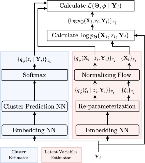
In the proposed method, to increase the expressive power of the approximate distributions $q_{\phi}(\mathbf{X}_{i}\mid z_{i},\mathbf{Y}_{i})$ and $q_{\phi}(z_{i}\mid\mathbf{Y}_{i})$, neural networks parameterized by $\phi$ are employed. Specifically, $q_{\phi}(\mathbf{X}_{i}\mid z_{i},\mathbf{Y}_{i})$ is a neural network containing normalizing flows, and $q_{\phi}(z_{i}\mid\mathbf{Y}_{i})$ is a neural network with a softmax activation function in the final layer.

By applying the re-parameterization trick, $\nabla_{\phi,\Theta}\text{ELBO}_{i}$ can be approximated as

$$\nabla_{(\phi,\Theta)}\text{ELBO}_{i}$$

$$=\nabla_{(\phi,\Theta)}E_{p(\mathbf{\epsilon})q_{\phi}(z_{i}\mid\mathbf{Y}_{i})}\left[f_{(\phi,\Theta)}(g_{\phi}(\mathbf{\epsilon},z_{i},\mathbf{Y}_{i}),z_{i})\right]$$

$$=E_{p(\mathbf{\epsilon})}\left[\nabla_{(\phi,\Theta)}\sum_{z_{i}=1}^{M}q_{\phi}(z_{i}\mid\mathbf{Y}_{i})f_{(\phi,\Theta)}(g_{\phi}(\mathbf{\epsilon},z_{i},\mathbf{Y}_{i}),z_{i})\right]$$

$$\approx\frac{1}{L}\sum_{l=1}^{L}\nabla_{(\phi,\Theta)}\sum_{z_{i}=1}^{M}q_{\phi}(z_{i}\mid\mathbf{Y}_{i})f_{(\phi,\Theta)}(g_{\phi}(\mathbf{\epsilon},z_{i},\mathbf{Y}_{i}),z_{i})$$

$$=\nabla_{(\phi,\Theta)}\frac{1}{L}\left[\sum_{l=1}^{L}\sum_{z_{i}=1}^{M}q_{\phi}(z_{i}\mid\mathbf{Y}_{i})f_{(\phi,\Theta)}(g_{\phi}(\mathbf{\epsilon},z_{i},\mathbf{Y}_{i}),z_{i})\right],$$ (15)

where $\mathbf{\epsilon}^{(l)}\sim p(\mathbf{\epsilon})$. As in [25], the number $L$ of Monte Carlo samples is 1 and $p(\mathbf{\epsilon})$ is the standard normal distribution in this paper. An overview of the proposed method is shown in Figure 1.

Figure 1: Overview of proposed method.

4.3 Estimating the Number of Clusters

The number of clusters is estimated using the Bayesian information criterion (BIC) as in [8, 10, 7]. The BIC is defined as

$$\text{BIC}=\log\,\mathrm{L}-\frac{1}{2}\bigl{(}\lVert P\rVert-1\bigr{)}\log\ N,$$

and a model with a larger BIC value is preferred. Here, $\mathrm{L}$ is the likelihood of a model, $\lVert P\lVert$ is the number of parameters of the model, and $N$ is the number of data. In MSSMs, the mean of $\text{ELBO}_{i}$ is used as $\mathrm{L}$, and the number of parameters of $\Theta$ referred to as $\lVert P_{\Theta}\lVert$ is used as $\lVert P\lVert$. Consequently, the BIC of the MSSMs is

$$\text{BIC}=\frac{1}{N}\sum_{i=1}^{N}\text{ELBO}_{i}-\dfrac{1}{2}\bigl{(}\lVert P_{\Theta}\rVert-1\bigr{)}\log\,N.$$ (16)

If the number of clusters is unknown, we train models with different numbers of clusters and adopt the model that exhibits the largest BIC.

4.4 Entropy Annealing

In parameter estimation of MSSMs, $q_{\phi}(z_{i}\mid\mathbf{Y}_{i})$ may concentrate on some clusters and converge to a local optimum in the early stages of training. To prevent this, we introduce an additional penalty term called entropy annealing. The loss function of the proposed method can be rewritten as

$$\mathcal{L} (\Theta,\phi\mid D_{\mathbf{Y}})=-\frac{1}{N}\sum_{i=1}^{N}\text{ELBO}_{i}$$

$$={} \frac{1}{N}\sum_{i=1}^{N}\left[-\mathcal{H}(q_{\phi}(z_{i}\mid\mathbf{Y}_{i}))-\sum_{z_{i}=1}^{M}q_{\phi}(z_{i}\mid\mathbf{Y}_{i})\mathcal{H}(q_{\phi}(\mathbf{X}_{i}\mid z_{i},\mathbf{Y}_{i}))\right.$$

$$\left.-\sum_{z_{i}=1}^{M}\int q_{\phi}(\mathbf{X}_{i},z_{i}\mid\mathbf{Y}_{i})\log p_{\theta^{(k)}}(\mathbf{X}_{i},z_{i},\mathbf{Y}_{i})\operatorname{d\!}\mathbf{X}_{i}\right],$$ (17)

where $\mathcal{H}(q)$ indicates the entropy of $q$. From Equation (17), the loss function comprises the entropy penalty term concerning the approximate distribution and the expected value of the complete data log-likelihood. Entropy annealing increases the entropy penalty $\mathcal{H}(q_{\phi}(z_{i}\mid\mathbf{Y}_{i}))$ in the early stages of training, which prevents $q_{\phi}(z_{i}\mid\mathbf{Y}_{i})$ from converging to the local optimum. The loss function with entropy annealing is

$$\mathcal{L}^{{}^{\prime}}_{n} (\Theta,\phi\mid\mathbf{Y}_{i})=\mathcal{L}(\Theta,\phi\mid\mathbf{Y}_{i})-{\alpha_{n}}\mathcal{H}(q_{\phi}(k|\mathbf{Y}_{i})),$$ (18)

where ${\alpha_{n}}$ is the strength of entropy annealing at epoch $n$.

The strength ${\alpha_{n}}$ is dynamically changed by epoch as

$$\alpha_{n}=\begin{cases}\alpha&\text{if }1\leq n<n_{\alpha}^{\text{start}},\\ \frac{n_{\alpha}^{\text{end}}-n}{n_{\alpha}^{\text{end}}-n_{\alpha}^{\text{start}}}a_{0}&\text{if }n_{\alpha}^{\text{start}}\leq n<n_{\alpha}^{\text{end}},\\ 0&\text{if }n_{\alpha}^{\text{end}}\leq n,\end{cases}$$ (19)

where $\alpha$, $n_{\alpha}^{\text{start}}$, and $n_{\alpha}^{\text{end}}$ are the maximum annealing strength, number of epochs at which entropy annealing starts to weaken, and number of epochs at which entropy annealing ends, respectively. Other tricks to avoid convergence to a local optimum are described in Appendix A.

5 Experiments

Table 1: Parameter values of Stuart–Landau oscillators.

Cluster	$a_{1}^{(k)}$	$a_{2}^{(k)}$	$b_{1}^{(k)}$	$b_{2}^{(k)}$	$\mathbf{A}^{(k)}$	$b^{(k)}$	$\mu_{x}^{(k)}$	$\mu_{y}^{(k)}$	$\mathbf{C}^{(k)}$
$1$	$1.0$	$0.5$	$0.5$	$0.1$	$0.05$ $\times\mathbf{I}_{2}$	$0.05$	$1.0$	$0.0$	$0.05$ $\times\mathbf{I}_{2}$
$2$	$1.0$	$1.5$	$0.8$	$0.2$	$0.05$ $\times\mathbf{I}_{2}$	$0.05$	$1.0$	$0.0$	$0.05$ $\times\mathbf{I}_{2}$
$3$	$1.0$	$1.0$	$0.2$	$0.0$	$0.05$ $\times\mathbf{I}_{2}$	$0.05$	$1.0$	$0.0$	$0.05$ $\times\mathbf{I}_{2}$

Table 2: Results of experiment for Stuart–Landau oscillator dataset. (a) Five-trial mean BIC values for different values of $M$. The values in parentheses are standard deviations. (b) Total confusion matrix obtained from five trials. (c) Five-trial mean of estimated parameter values. The values in parentheses are standard deviations.

(a) BIC values

$M$	2	3	4	5
BIC	$-107.32$ ($7.60$)	$25.83$ ($1.26$)	$-17.55$ ($0.73$)	$-61.85$ ($1.91$)

(b) Confusion matrix

True $\backslash$ Prediction	$1$	$2$	$3$
$1$ ($i=001,\;\dotsc\,,\;300$)	1500	0	0
$2$ ($i=301,\;\dotsc\,,\;600$)	0	1500	0
$3$ ($i=601,\;\dotsc\,,\;900$)	0	0	1500

(c) Estimated parameter values

Cluster	$p_{0}^{(k)}$	$a_{2}^{(k)}$	$b_{1}^{(k)}$	$b_{2}^{(k)}$	$\mathbf{A}_{11}^{(k)}$	$\mathbf{A}_{12}^{(k)}$	$\mathbf{A}_{22}^{(k)}$	$b^{(k)}$	$\mathbf{C}_{11}^{(k)}$	$\mathbf{C}_{12}^{(k)}$	$\mathbf{C}_{22}^{(k)}$	$\mu_{x}^{(k)}$	$\mu_{y}^{(k)}$
1	$0.334$ ($0.002$)	$0.499$ ($0.005$)	$0.497$ ($0.000$)	$0.097$ ($0.000$)	$0.077$ ($0.001$)	$0.000$ ($0.001$)	$0.071$ ($0.001$)	$0.026$ ($0.001$)	$0.079$ ($0.008$)	$0.018$ ($0.007$)	$0.060$ ($0.004$)	$1.030$ ($0.016$)	$0.006$ ($0.002$)
2	$0.333$ ($0.001$)	$1.492$ ($0.002$)	$0.795$ ($0.001$)	$0.189$ ($0.001$)	$0.084$ ($0.001$)	$0.010$ ($0.001$)	$0.075$ ($0.001$)	$0.021$ ($0.001$)	$0.045$ ($0.006$)	$-0.019$ ($0.003$)	$0.073$ ($0.003$)	$0.985$ ($0.007$)	$-0.002$ ($0.002$)
3	$0.333$ ($0.002$)	$0.990$ ($0.000$)	$0.201$ ($0.000$)	$0.001$ ($0.000$)	$0.082$ ($0.002$)	$-0.002$ ($0.001$)	$0.072$ ($0.001$)	$0.023$ ($0.000$)	$0.058$ ($0.008$)	$-0.004$ ($0.008$)	$0.069$ ($0.003$)	$0.910$ ($0.086$)	$0.002$ ($0.003$)

(a) Actual time series

(b) Estimated latent variables

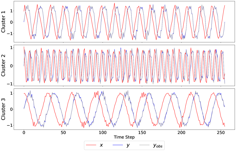
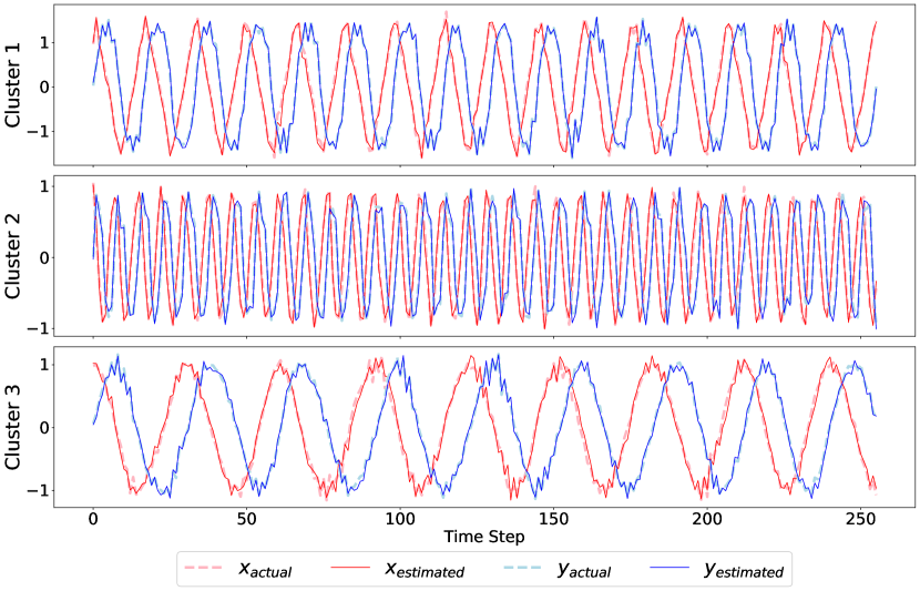
Figure 2: Representative samples of the actual and estimated time series for the Stuart–Landau oscillator dataset. (a) Actual time series. The latent variable $y$ is observed as $y_{\text{obs}}$ under noise. (b) Estimated latent variables. For comparison, the actual latent variables are also plotted.

Table 3: Parameter values of SIR models.

Cluster	$\beta^{(k)}$	$\gamma^{(k)}$	$a^{(k)}$	$b^{(k)}$	$c^{(k)}$	$\bm{\rho}_{\text{(}{\text{init}})}^{(k)}$
$1$	$0.9$	$0.1$	$3$	$3$	$2$	$(0.95,0.04,0.01)$
2	0.3	0.05	3	3	2	$(0.95,0.04,0.01)$

Table 4: Results of experiment for SIR model dataset. (a) Five-trial mean BIC values for different values of $M$. The values in parentheses are standard deviations. (b) Total confusion matrix obtained from five trials. (c) Five-trial mean of estimated parameter values. The values in parentheses are standard deviations.

(a) BIC values

Number of clusters	$2$	$3$	$4$
BIC	$102.04$ ($0.36$)	$71.30$ ($0.31$)	$40.81$ ($0.30$)

(b) Confusion matrix

Cluster $\backslash$ Prediction	$1$	$2$
$1$ ($i=001,\;\dotsc\,,\;300$)	$1500$	$0$
$2$ ($i=301,\;\dotsc\,,\;600$)	$0$	$1500$

(c) Estimated parameter values

Cluster	$p_{0}^{(k)}$	$\beta^{(k)}$	$\gamma^{(k)}$	$a^{(k)}$	$b^{(k)}$	$c^{(k)}$	$\bm{\rho}_{(S,\text{init})}^{(k)}$	$\bm{\rho}_{(I,\text{init})}^{(k)}$	$\bm{\rho}_{(R,\text{init})}^{(k)}$
$1$	$0.501$ ($0.002$)	$0.851$ ($0.001$)	$0.101$ ($0.000$)	$2.801$ ($0.014$)	$2.980$ ($0.010$)	$2.686$ ($0.043$)	$0.954$ ($0.002$)	$0.037$ ($0.000$)	$0.009$ ($0.002$)
$2$	$0.499$ ($0.002$)	$0.293$ ($0.003$)	$0.049$ ($0.001$)	$2.763$ ($0.006$)	$3.049$ ($0.007$)	$2.715$ ($0.007$)	$0.930$ ($0.013$)	$0.037$ ($0.000$)	$0.034$ ($0.013$)

(a) Actual time series

(b) Estimated latent variables

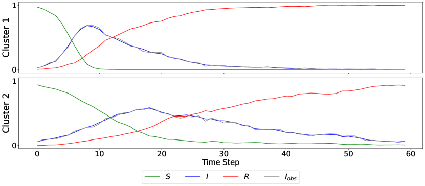
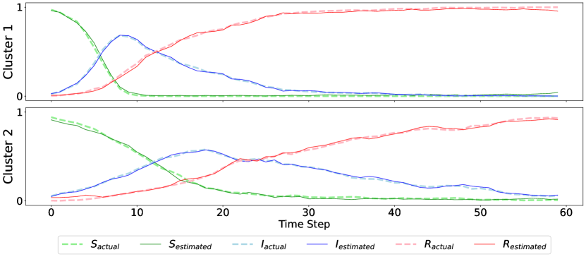
Figure 3: Representative samples of the actual and estimated time series for the SIR model dataset. (a) Actual time series. The latent variable $I$ is observed as $I_{\text{obs}}$ under noise. (b) Estimated latent variables. For comparison, the actual latent variables are also plotted.

We demonstrate via experiments on simulated datasets that the proposed method is effective for clustering, parameter estimation, and estimating the number of clusters. Specifically, datasets are generated from two dynamics: the Stuart–Landau oscillator [26] and the SIR model [27]. The code is available at https://github.com/ryoichi0917/svi_mssm.

In our experiments, we use the residual flows [28, 29] as the architecture of the normalizing flows. This is because the residual flows have highly expressive power compared to other normalizing flow architectures, such as MADE [30] and MAF [31].

5.1 Stuart–Landau Oscillator

Firstly, we apply the proposed method to time series generated by a discrete-time stochastic version of the Stuart–Landau oscillator. The discrete-time stochastic Stuart–Landau oscillator belonging to the $k$-th cluster is defined as

$$x{[t+1]}={} x{[t]}+a_{1}^{(k)}x{[t]}-b_{1}^{(k)}y{[t]}$$

$$-\left(x{[t]}^{2}+y{[t]}^{2}\right)\left(a_{2}^{(k)}x{[t]}-b_{2}^{(k)}y{[t]}\right)+\xi_{x},$$ (20a)

$$y{[t+1]}={} y{[t]}+a_{1}^{(k)}y{[t]}+b_{1}^{(k)}x{[t]}$$

$$-\left(x{[t]}^{2}+y{[t]}^{2}\right)\left(a_{2}^{(k)}y{[t]}+b_{2}^{(k)}x{[t]}\right)+\xi_{y},$$ (20b)

$$y_{\text{obs}}{[t]}={} y{[t]}+\xi_{\text{obs}},$$ (20c)

where

$$\begin{bmatrix}\xi_{x}&\xi_{y}\end{bmatrix}^{\top} \sim\mathcal{N}\Bigl{(}0,\mathbf{A}^{(k)}{\mathbf{A}^{(k)}}^{\top}\Bigr{)},$$ (21a)

$$\xi_{\text{obs}} \sim\mathcal{N}\Bigl{(}0,{b^{(k)}}^{2}\Bigr{)},$$ (21b)

$$\begin{bmatrix}x{[1]}&y{[1]}\end{bmatrix}^{\top} \sim\mathcal{N}\Bigl{(}\begin{bmatrix}\mu_{x}^{(k)}&\mu_{y}^{(k)}\end{bmatrix}^{\top},\mathbf{C^{(k)}}{\mathbf{C}^{(k)}}^{\top}\Bigr{)},$$ (21c)

and $\mathbf{A}^{(k)}$ and $\mathbf{C}^{(k)}$ are lower triangular matrices. The parameter $a_{1}^{(k)}$ is assumed to be given to ensure the uniqueness of the latent variables. Thus, the parameters to be estimated are $\theta^{(k)}_{Q}=\{a_{2}^{(k)},b_{1}^{(k)},b_{2}^{(k)},\mathbf{A}^{(k)}\}$, $\theta^{(k)}_{R}=\{b^{(k)}\}$, and $\theta^{(k)}_{P_{0}}=\{\mu_{x}^{(k)},\mu_{y}^{(k)},\mathbf{C}^{(k)}\}$.

The number of clusters was set to three, which means that the dataset is generated from three different Stuart–Landau oscillators. The parameters of each Stuart–Landau oscillator are shown in Table 1, and representative samples of the Stuart Landau oscillator dataset are shown in Figure 22. The number of time series belonging to each cluster was 300. Details of the hyperparameters, such as the configuration of the approximate distribution and optimizer settings, are provided in Appendix B.1.

The values of BIC for the MSSMs with from two to five clusters are shown in Table 2(c)2(a). BIC is the largest when the number of clusters is three, which is the correct number of clusters. Table 2(c)2(b) is the confusion matrix that shows the result of clustering. This result indicates that perfect clustering is achieved.

Table 2(c)2(c) shows the estimated values of the MSSM parameters. From the table, the estimated values are close to the true values for most of the parameters. Figure 22 shows the actual and estimated latent variables. From the figure, the proposed method accurately estimates the latent variables.

5.2 SIR Model

Secondly, we apply the proposed method to time series generated by a discrete-time stochastic version of the SIR model [32]. The discrete-time stochastic SIR model belonging to the $k$-th cluster is defined as

$$\bm{\rho}[t+1]\mid\bm{\rho}[t] \sim\text{Dirichlet}(10^{{a}^{(k)}}\bm{f}^{(k)}(\bm{\rho}[t])),$$ (22a)

$$I_{\text{obs}}[t]\mid\rho_{(I)}[t] \sim\text{Beta}(10^{{b}^{(k)}}\rho_{(I)}[t],10^{{b}^{(k)}}(1-\rho_{(I)}[t])),$$ (22b)

$$\bm{\rho}[1] \sim\text{Dirichlet}(10^{{c}^{(k)}}\bm{\rho}_{(\text{init})}^{(k)}),$$ (22c)

where

$$\bm{f}^{(k)}(\bm{\rho}[t])=\begin{bmatrix}f_{(S)}^{(k)}(\bm{\rho}[t]),f_{(I)}^{(k)}(\bm{\rho}[t]),f_{(R)}^{(k)}(\bm{\rho}[t])\end{bmatrix}^{\top},$$ (23a)

$$\left.\begin{aligned} f_{(S)}^{(k)}(\bm{\rho}[t])&=\rho_{(S)}[t]-\beta^{(k)}\rho_{(S)}[t]\rho_{(I)}[t],\\ f_{(I)}^{(k)}(\bm{\rho}[t])&=\rho_{(I)}[t]+\beta^{(k)}\rho_{(S)}[t]\rho_{(I)}[t]-\gamma^{(k)}\rho_{(I)}[t],\\ f_{(R)}^{(k)}(\bm{\rho}[t])&=\rho_{(R)}[t]+\gamma^{(k)}\rho_{(I)}[t],\end{aligned}\quad\right\}$$ (23b)

$$\bm{\rho}{[t]}=\begin{bmatrix}\rho_{(S)}[t],\rho_{(I)}[t],\rho_{(R)}[t]\end{bmatrix}^{\top},$$ (23c)

$$\bm{\rho}_{(\text{init})}^{(k)}=\begin{bmatrix}\rho_{(S,\text{init})}^{(k)},\rho_{(I,\text{init})}^{(k)},\rho_{(R,\text{init})}^{(k)}\end{bmatrix}^{\top},$$ (23d)

$$\rho_{(S,\text{init})}^{(k)}+\rho_{(I,\text{init})}^{(k)}+\rho_{(R,\text{init})}^{(k)}=1.$$ (23e)

Thus, the parameters to be estimated are $\theta^{(k)}_{Q}=\{\beta^{(k)},\gamma^{(k)},a^{(k)}\}$, $\theta^{(k)}_{R}=\{b^{(k)}\}$, and $\theta^{(k)}_{P_{0}}=\{c^{(k)},\bm{\rho}_{(init)}^{(k)}\}$. Although the SIR model (22) is intractable for normalizing flows due to the Dirichlet distributions, we can apply the proposed method by rewriting Eq. (22) into an equivalent form. See Appendix B.2 for details.

The number of clusters was set to two, which means that the dataset is generated from two different SIR models. The parameters of each SIR model are shown in Table 3, and representative samples of the SIR model dataset are shown in Figure 33. The number of time series belonging to each cluster was 300. Details of the hyperparameters, such as the configuration of the approximate distribution and optimizer settings, are provided in Appendix B.1.

The values of BIC for the MSSMs with from two to four clusters are shown in Table 4(c)4(a). BIC is the largest when the number of clusters is two, which is the correct number of clusters. Table 4(c)4(b) is the confusion matrix that shows the result of clustering. This result indicates that perfect clustering is achieved.

Table 4(c)4(c) shows the estimated values of the MSSM parameters. From the table, the estimated values are close to the true values for most of the parameters. Figure 33 shows the actual and estimated latent variables. From the figure, the proposed method accurately estimates the latent variables.

6 Conclusion

In this paper, we propose a novel method of model-based time series clustering with mixtures of general state-space models. An advantage of the proposed method is that it enables the use of tailored time series models. This not only improves clustering and prediction accuracy but also enhances the interpretability of the estimated parameters. Experiments on simulated datasets show that the proposed method is effective for clustering, parameter estimation, and estimating the number of clusters.

A limitation of this study is that the validation experiments in this paper were only conducted on simulated datasets. Future research should validate the effectiveness of the proposed method on real datasets. When applying the proposed method to real data, it would also be useful to enhance the structure of the MSSMs to allow for the input of exogenous variables.

Appendix A Practical Efforts for Parameter Optimization

In this section, we describe three tricks to avoid undesirable convergence of $q_{\phi}(z_{i}\mid\mathbf{Y}_{i})$ to a local optimum, other than entropy annealing.

The first of these tricks relates to the optimizer. In the proposed method, (simple) mini-batch SGD is used to optimize MSSMs. This is because mini-batch SGD can accurately approximate the posterior distribution in SVI [1]. The learning rate of mini-batch SGD is changed periodically based on cyclical learning rates [2] to avoid convergence to a local optimum.

The second is to introduce learning rate scheduling and fine-tuning. When MSSMs are trained with cyclical learning rates, the parameters do not converge, because the learning rate increases periodically. Therefore, we set the learning rate to a low value at the late stages of the training to make the parameters converge. After this training, fine-tuning is performed to learn only $\theta^{(k)}_{P_{0}}$ and parameters of normalizing flow modules. This is because $\theta^{(k)}_{P_{0}}$ is poorly optimized if all parameters are simultaneously learned. The loss function is significantly less affected by the improvement of $\theta^{(k)}_{P_{0}}$ than by that of $\theta^{(k)}_{R}$ due to the fact

$$\log p_{\mathbf{\theta}_{P_{0}^{(k)}},\mathbf{\theta}_{R^{(k)}}}(\mathbf{X}_{i}\mid z_{i}=k)$$

$$=\log p_{\mathbf{\theta}_{P_{0}^{(k)}}}(\mathbf{x}_{i}[t]\mid z_{i}=k)+\sum_{t=2}^{T}\log p_{\mathbf{\theta}_{R^{(k)}}}(\mathbf{x}_{i}[t+1]\mid\mathbf{x}_{i}[t],z_{i}=k).$$ (24)

Finally, we train MSSMs multiple times from different initial parameter values and adopt the model with the lowest loss to avoid rare cases unsolved by the above-mentioned two tricks.

With the above tools and entropy annealing, MSSMs converged without falling into local optimum solutions in the experiments.

Appendix B Details of Experiments

B.1 Model Architecture

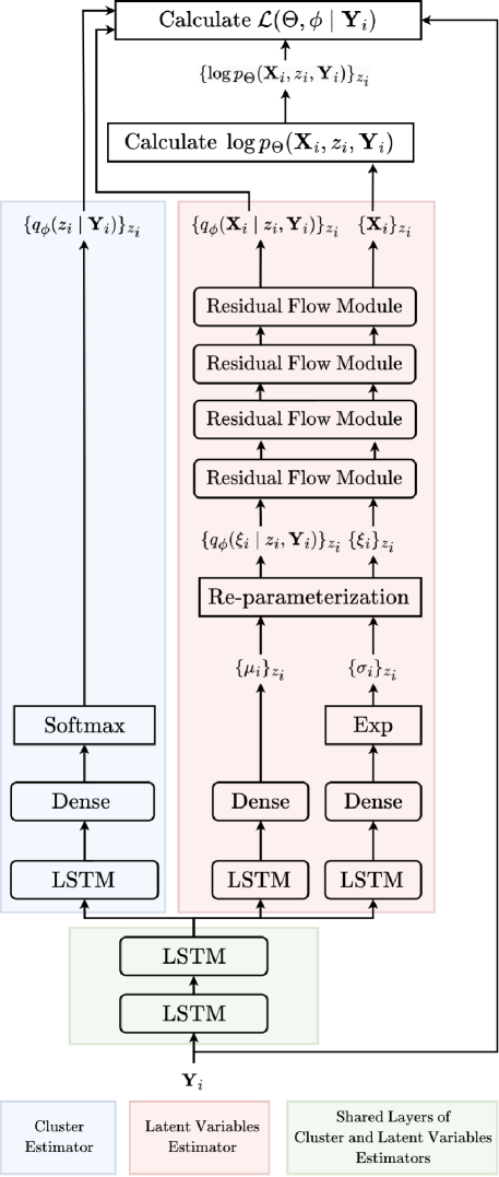
Figure 4: Details of model architecture.

The architectural details of the model used in our experiments are shown in Figure 4. For the hyperparameter settings of each layer, see the code on GitHub (https://github.com/ryoichi0917/svi_mssm).

B.2 Equivalent form of the SIR Model

For the stochastic SIR model, the representation (22) is intractable for normalizing flows due to the Dirichlet distribution. Nevertheless, we can apply the proposed method by rewriting the model in the equivalent form as

$$\left.\begin{aligned} G_{(S)}[t+1]\sim\text{Gamma}(10^{{a}^{(k)}}f_{(S)}^{(k)}(\bm{\rho}[t]),1),\\ G_{(I)}[t+1]\sim\text{Gamma}(10^{{a}^{(k)}}f_{(I)}^{(k)}(\bm{\rho}[t]),1),\\ G_{(R)}[t+1]\sim\text{Gamma}(10^{{a}^{(k)}}f_{(R)}^{(k)}(\bm{\rho}[t]),1),\end{aligned}\quad\right\}$$ (25a)

$$I_{\text{obs}}[t]\mid\rho_{(I)}[t]\sim\text{Beta}(10^{{b}^{(k)}}\rho_{(I)}[t],10^{{b}^{(k)}}(1-\rho_{(I)}[t])),$$ (25b)

$$\left.\begin{aligned} G_{(S)}[1]&\sim\text{Gamma}(10^{{c}^{(k)}}\rho_{(S,\text{init})}^{(k)},1),\\ G_{(I)}[1]&\sim\text{Gamma}(10^{{c}^{(k)}}\rho_{(I,\text{init})}^{(k)},1),\\ G_{(R)}[1]&\sim\text{Gamma}(10^{{c}^{(k)}}\rho_{(R,\text{init})}^{(k)},1),\end{aligned}\quad\right\}$$ (25c)

where

$$\left.\begin{aligned} f_{(S)}^{(k)}(\bm{\rho}[t])&=\rho_{(S)}[t]-\beta^{(k)}\rho_{(S)}[t]\rho_{(I)}[t],\\ f_{(I)}^{(k)}(\bm{\rho}[t])&=\rho_{(I)}[t]+\beta^{(k)}\rho_{(S)}[t]\rho_{(I)}[t]-\gamma^{(k)}\rho_{(I)}[t],\\ f_{(R)}^{(k)}(\bm{\rho}[t])&=\rho_{(R)}[t]+\gamma^{(k)}\rho_{(I)}[t],\end{aligned}\quad\right\}$$ (26a)

$$\left.\begin{aligned} \rho_{(S)}[t]&=\frac{G_{(S)}[t]}{G_{(S)}[t]+G_{(I)}[t]+G_{(R)}[t]},\\ \rho_{(I)}[t]&=\frac{G_{(I)}[t]}{G_{(S)}[t]+G_{(I)}[t]+G_{(R)}[t]},\\ \rho_{(R)}[t]&=\frac{G_{(R)}[t]}{G_{(S)}[t]+G_{(I)}[t]+G_{(R)}[t]},\end{aligned}\quad\right\}$$ (26b)

$$\bm{\rho}{[t]}=\begin{bmatrix}\rho_{(S)}[t],\rho_{(I)}[t],\rho_{(R)}[t]\end{bmatrix}^{\top},$$ (26c)

$$\rho_{(S,\text{init})}^{(k)}+\rho_{(I,\text{init})}^{(k)}+\rho_{(R,\text{init})}^{(k)}=1.$$ (26d)

References

• [1] S. Rani, G. Sikka, Recent techniques of clustering of time series data: A Survey, International Journal of Computer Applications 52 (15) (2012) 1–9.
• [2] S. Aghabozorgi, A. S. Shirkhorshidi, T. Y. Wah, Time-series clustering – A decade review, Information Systems 53 (2015) 16–38. doi:10.1016/j.is.2015.04.007.
• [3] H. He, Y. Tan, Automatic pattern recognition of ECG signals using entropy-based adaptive dimensionality reduction and clustering, Applied Soft Computing 55 (2017) 238–252. doi:10.1016/j.asoc.2017.02.001.
• [4] M. L. Mitchell, J. H. Mulherin, The impact of industry shocks on takeover and restructuring activity, Journal of Financial Economics 41 (2) (1996) 193–229. doi:10.1016/0304-405X(95)00860-H.
• [5] L. Owsley, L. Atlas, G. Bernard, Automatic clustering of vector time-series for manufacturing machine monitoring, in: 1997 IEEE International Conference on Acoustics, Speech, and Signal Processing, Vol. 4, 1997, pp. 3393–3396. doi:10.1109/ICASSP.1997.595522.
• [6] T. Warren, Liao, Clustering of time series data – A survey, Pattern Recognition 38 (11) (2005) 1857–1874. doi:10.1016/j.patcog.2005.01.025.
• [7] R. Umatani, T. Imai, K. Kawamoto, S. Kunimasa, Time series clustering with an EM algorithm for mixtures of linear Gaussian state space models, Pattern Recognition 138 (2023) 109375. doi:10.1016/j.patcog.2023.109375.
• [8] Y. Xiong, D.-Y. Yeung, Time series clustering with ARMA mixtures, Pattern Recognition 37 (8) (2004) 1675–1689. doi:10.1016/j.patcog.2003.12.018.
• [9] B. V. Kini, C. C. Sekhar, Bayesian mixture of AR models for time series clustering, Pattern Analysis and Applications 16 (2) (2013) 179–200. doi:10.1007/s10044-011-0247-5.
• [10] C. Li, G. Biswas, A bayesian approach to temporal data clustering using hidden Markov models., in: Proceedings of the Seventeenth International Conference on Machine Learning, 2000, pp. 543–550.
• [11] G. Kitagawa, Non-Gaussian state-space modeling of nonstationary time series, Journal of the American Statistical Association 82 (400) (1987) 1032–1041. doi:10.2307/2289375.
• [12] H. Tanizaki, R. S. Mariano, Nonlinear and non-Gaussian state-space modeling with Monte Carlo simulations, Journal of Econometrics 83 (1) (1998) 263–290. doi:10.1016/S0304-4076(97)80226-6.
• [13] G. J. McLachlan, K. E. Basford, Mixture Models: Inference and Applications to Clustering, Vol. 38, 1988. doi:10.2307/2348072.
• [14] M. D. Hoffman, D. M. Blei, C. Wang, J. Paisley, Stochastic variational inference, Journal of Machine Learning Research 14 (40) (2013) 1303–1347.
• [15] C. M. Bishop, Pattern Recognition and Machine Learning, Springer, 2006.
• [16] M. J. Beal, Variational algorithms for approximate Bayesian inference, Doctoral, University College London (2003).
• [17] D. J. Rezende, S. Mohamed, Variational inference with normalizing flows, in: Proceedings of the 32nd International Conference on International Conference on Machine Learning - Volume 37, ICML’15, JMLR.org, Lille, France, 2015, pp. 1530–1538.
• [18] G. Papamakarios, E. Nalisnick, D. J. Rezende, S. Mohamed, B. Lakshminarayanan, Normalizing flows for probabilistic modeling and inference, The Journal of Machine Learning Research 22 (57) (2021) 1–64.
• [19] S. Fröhwirth-Schnatter, S. Kaufmann, Model-based clustering of multiple time series, Journal of Business & Economic Statistics 26 (1) (2008) 78–89. doi:10.1198/073500107000000106.
• [20] B. A. Wilcox, F. Hamano, Kalman’s expanding influence in the econometrics discipline, IFAC-PapersOnLine 50 (1) (2017) 637–644. doi:10.1016/j.ifacol.2017.08.106.
• [21] D. P. Kingma, T. Salimans, R. Jozefowicz, X. Chen, I. Sutskever, M. Welling, Improved variational inference with inverse autoregressive flow, in: Advances in Neural Information Processing Systems, Vol. 29, Curran Associates, Inc., 2016.
• [22] N. Foti, J. Xu, D. Laird, E. Fox, Stochastic variational inference for hidden Markov models, in: Advances in Neural Information Processing Systems, Vol. 27, Curran Associates, Inc., 2014.
• [23] J. Povala, I. Kazlauskaite, E. Febrianto, F. Cirak, M. Girolami, Variational Bayesian approximation of inverse problems using sparse precision matrices, Computer Methods in Applied Mechanics and Engineering 393 (2022) 114712. doi:10.1016/j.cma.2022.114712.
• [24] H. Xuan, L. Maestrini, F. Chen, C. Grazian, Stochastic variational inference for GARCH models, Statistics and Computing 34 (1) (2023) 45. doi:10.1007/s11222-023-10356-7.
• [25] D. P. Kingma, M. Welling, Auto-Encoding Variational Bayes (2013). arXiv:1312.6114, doi:10.48550/arXiv.1312.6114.
• [26] L. D. Landau, On the problem of turbulence, Proceedings of the USSR Academy of Sciences 44 (1944). doi:10.1016/b978-0-08-010586-4.50057-2.
• [27] W. O. Kermack, A. G. McKendrick, A contribution to the mathematical theory of epidemics, Proceedings of the Royal Society of London. Series A, Containing papers of a mathematical and physical character 115 (772) (1927) 700–721.
• [28] J. Behrmann, W. Grathwohl, R. T. Q. Chen, D. Duvenaud, J.-H. Jacobsen, Invertible residual networks, in: K. Chaudhuri, R. Salakhutdinov (Eds.), Proceedings of the 36th International Conference on Machine Learning, Vol. 97 of Proceedings of Machine Learning Research, PMLR, 2019-06-09/2019-06-15, pp. 573–582.
• [29] R. T. Q. Chen, J. Behrmann, D. K. Duvenaud, J.-H. Jacobsen, Residual flows for invertible generative modeling, in: Advances in Neural Information Processing Systems, Vol. 32, Curran Associates, Inc., 2019.
• [30] B. Uria, M.-A. Côté, K. Gregor, I. Murray, H. Larochelle, Neural autoregressive distribution estimation, Journal of Machine Learning Research 17 (205) (2016) 1–37.
• [31] G. Papamakarios, T. Pavlakou, I. Murray, Masked autoregressive flow for density estimation, in: Advances in Neural Information Processing Systems, Vol. 30, Curran Associates, Inc., 2017.
• [32] D. Osthus, K. S. Hickmann, P. C. Caragea, D. Higdon, S. Y. Del Valle, Forecasting seasonal influenza with a state-space SIR model, The Annals of Applied Statistics 11 (LA-UR-15-26537) (2017). doi:10.1214/16-AOAS1000.
• [1] S. Mandt, M. D. Hoffman, D. M. Blei, Stochastic gradient descent as approximate Bayesian inference, Journal of Machine Learning Research 18 (134) (2017) 1–35.
• [2] L. N. Smith, Cyclical Learning Rates for Training Neural Networks, in: 2017 IEEE Winter Conference on Applications of Computer Vision (WACV), 2017, pp. 464–472. doi:10.1109/WACV.2017.58.