Recovery of synchronized oscillations on multiplex networks by tuning dynamical time scales

Abstract

The heterogeneity among interacting dynamical systems or in the pattern of interactions observed in real complex systems, often lead to partially synchronized states like chimeras or oscillation suppressed states like inhomogeneous or homogeneous steady states. In such cases, recovering synchronized oscillations back is required in many applications but is a real challenge. We present how synchronized oscillations can be restored by tuning the dynamical time scales of the system. For this we use the model of a multiplex network where first layer of coupled oscillators is multiplexed with an environmental layer that can generate various possible chimera states and suppressed states. We show that by tuning the time scale mismatch between the layers , we can revive synchronized oscillations in both layers from these states. We analyse the nature of the transition to synchronization and the results are verified for two- and three-layer multiplex networks.

[first]Indian Institute of Science Education and Research Tirupati, Tirupati-517 619, India

[second]Indian Institute of Technology Indore, Khandwa Road, Simrol, Indore-453 552, India

[third]Indian Institute of Science Education and Research Thiruvananthapuram, Thiruvananthapuram-695 551, India

1 Introduction

The collective phenomena emerging from the interactions of multiple dynamical systems are intensely studied recently and they have a wide range of applications in physics, biology, chemistry, technology, and social sciences. In such studies, the framework of complex networks is effectively utilized to model the complex pattern of interactions [1]. However, the variability and heterogeneity of the interacting subsystems and the different types of interactions are best studied using the model of multiplex networks [2, 3]. These have wider applications since multiplexing can be between layers of different topology or with different intrinsic dynamics for the subsystems[4]. Hence, they are found to be most effective in studying biological systems [5, 6], social interactions [7], power grids [8], neuron-glia networks [9] and epidemiology [10].

The emergent dynamics on multiplex networks are rich with several interesting phenomena like diverse forms of synchronization [11], cluster synchronization [12], amplitude death [13], and oscillation death [14, 15]. Also, partially synchronized states, like different types of chimera [16, 17, 18], form an interesting spatiotemporal behaviour where spatially coherent and incoherent behaviour of states coexist in the system. Such chimera states emerge due to heterogeneities, either natural or induced [19], like parameter or frequency mismatch, coupling types [20], coupling delay [21, 22], time scale mismatch [23] and environment coupling [4]. Recently, the concept of chimeras is applied to explain many real-world phenomena such as epileptic seizures[24], brain activity of various aquatic animals[25] and power grid anomalies [26]. The wide variety of interesting emergent states related to chimera include amplitude-mediated chimera [27], amplitude chimera [28], breathing chimera [29], homogeneous steady state, inhomogeneous steady state, two-cluster steady state, multi-cluster steady state, and chimera death states [30, 31] such as one-state chimera death, two-state chimera death, etc.

The heterogeneity required for inducing chimera states can be explicitly added among interacting systems by considering them on multiplex networks and a few such studies are reported recently [32]. They include the activation and inhibition of chimera states through multiplexing [33], the presence of chimeras in a multilayer structure of neuronal networks [34], and the synchronization of chimeras in multiplex networks [35]. It is reported that weak multiplexing can induce chimera states in neural networks [36]. Additionally, the different synchronization scenarios in the multiplex network are widely studied [39], specifically the effect of inter-layer coupling delay [37, 38], explosive synchronization [40, 41, 42], synchronization in adaptive multiplex [43] and relay synchronization [44, 45]

We note that the two-layer nature of multiplex networks is useful in studying control strategies by which emergent dynamics can be controlled to desired states even when heterogeneities exist. The advantage of control schemes based on multiplexing is that they allow the desired state to be achieved in a certain layer by tuning the other layer which may be more accessible in practice. In this context, controlling the system back to synchronised states from oscillation suppressed states or chimera states will have many applications since synchronised states are desirable for the functionality of many systems like power distribution systems [46], brain activity [47], coupled laser systems and cardiac cells[48].

Recent studies report the various collective dynamics possible in oscillators that interact with each other through a dynamic environment in two-layer multiplex networks. In such systems, due to feedback from the other layer that is nonlocal in connectivity, a variety of emergent states like amplitude chimera, chimera death states, oscillation suppressed states, multi-cluster steady state etc can occur for different ranges of coupling strengths [4].

Multiple-time-scale phenomena are ubiquitous in nature and observed in temporal neural dynamics [49, 50], hormonal regulation [51, 52], chemical reactions [53], turbulent flows [54], and population dynamics [55]. When such systems are modeled by complex networks, the interplay between time scales and the structural properties of the network of nonlinear oscillators can generate many interesting phenomena like amplitude death [56], cluster synchronization [57, 58], and frequency synchronization [23]. Among interacting systems, if some systems have slower dynamics than others, their dynamics can be modelled on a multiplex network with the different layers evolving at different time scales.

In this study we consider the evolution of emergent states in a multiplex network and present how synchronized oscillations can be restored by tuning the dynamical time scales of the system. We illustrate this using the model of a multiplex network where the first layer of coupled oscillators is multiplexed with an environmental layer. In studies reported so far, the time scale mismatch among systems is shown to drive the systems to suppression of oscillations [56]. But we show that by tuning the time scale mismatch between the layers, we can restore synchronized oscillations in both layers from chimera or death states. We analyse the nature of the transition to synchronization, and the results are verified for two- and three-layer multiplex networks, with the Stuart-Landau (SL) oscillator as the nodal dynamics controlled by the environmental layer.

2 Two layer system

We start by considering a two layer multiplex system, with one layer comprising of a ring network of SL oscillators, referred to as the system layer, L1, which has local intra layer diffusive coupling. The second layer L2, which is the environment layer, is modeled as a ring network of 1-d over damped oscillators with intra layer diffusive couplings. The $N$ oscillators in L1 are connected to those in L2 via interlayer coupling of the feedback type and together they form a multiplex network. The dynamics of the environment L2 is sustained by the negative feedback from L1, and the dynamics of L1 is controlled by L2 via its positive feedback coupling. The dynamical equations for such a two-layer multiplex network are as given below.

$$\dot{x}_{i} = (1-x_{i}^{2}-y_{i}^{2})x_{i}-\omega y_{i}+\frac{K_{1}}{2P_{1}}\sum_{j=i-P_{1}}^{i+P_{1}}(x_{j}-x_{i})+\epsilon s_{i}$$

$$\dot{y}_{i} = (1-x_{i}^{2}-y_{i}^{2})y_{i}+\omega x_{i}$$

$$\dot{s}_{i} = \tau[-\gamma s_{i}-\epsilon x_{i}+\frac{K_{2}}{2P_{2}}\sum_{j=i-P_{2}}^{i+P_{2}}(s_{j}-s_{i})]$$ (1)

where the dynamics of SL oscillators in layer L1 are characterized by the variables $x_{i}$ and $y_{i}$ for i = 1, 2, …, N, and $\omega$ is the natural frequency of their intrinsic limit cycle oscillations. The 1-d over damped oscillators, $s_{i}$, in L2 have a positive damping coefficient, $\gamma$. The interaction between the layers is through feedback coupling of strength $\epsilon$. The interactions among the SL oscillators in the first layer are regulated by the intra-layer coupling strength, $K_{1}$, and coupling range, $P_{1}$, while that of the environment is controlled by $K_{2}$ and $P_{2}$. Here $P$ corresponds to the number of nearest neighbors in each direction; hence, $P\in\{1,\frac{N}{2}\}$, with $P=1$ for local connections, $P=\frac{N}{2}$ for a global coupling, for other cases $P$ is in the range $1<P<\frac{N}{2}$. The parameter $\tau$ is introduced to represent the mismatch in dynamical time scales between the two layers. Thus a value of $\tau<1$ means the environment layer L2 evolves at a slower time scale compared to layer L1.

Initially we keep $\tau=1$ so that both layers evolve with the same time scale. Following the recent study [4], we generate various emergent dynamical states in the system by varying the value of $\epsilon$, such as amplitude chimera(AC), homogeneous steady state(HSS), in homogeneous steady state(IHSS), one-state chimera death(1-CD), two-state chimera death(2-CD) etc. For this, we choose appropriate cluster-like initial conditions, for the $N=100$ oscillators in L1, while the systems in L2 start with random initial conditions[4].

Figure 1: Spatio temporal dynamics for different values of $\epsilon$ and $\tau$. (a1): Amplitude chimera at $\epsilon=2$ and $\tau=1$, (a2) and (a3): Synchronized oscillations at $\epsilon=2$, $\tau=0.4$ and $0.1$ respectively, (b1): Inhomogeneous steady state at $\epsilon=3$ and $\tau=1$, (b2) and (b3): Synchronized oscillations at $\epsilon=3$ and $\tau=0.4$ and $0.1$, (c1) and (c2): Homogeneous steady state at $\epsilon=4.5$, $\tau=1$ and $0.4$, (c3): Synchronized oscillations at $\epsilon=4.5$ and $\tau=0.1$, (d1): One state chimera death at $\epsilon=6.15$ and $\tau=1$, (d2): Homogeneous steady state at $\epsilon=6.15$ and $\tau=0.4$ and (d3): Synchronized oscillations at $\epsilon=6.15$ and $\tau=0.1$. The other parameter values used are : $K_{1}=K_{2}=10$, $P_{1}=1$, $P_{2}=25$, $\omega=2$ and $\gamma=1$

2.1 Recovery of synchronized oscillations

In this section, we present the role of time scale separation between the layers in controlling the emergent dynamics of the system. Specifically, we show how introducing a disparity in the time scale between the layers can facilitate the recovery of synchronized oscillations from the above-mentioned dynamical states. We consider the scenario in which all SL oscillators in L1 are connected with one another locally, $P_{1}=1$. At the same time, the environment is coupled nonlocally, with $P_{2}=25$. We set the values of $K_{1}$ and $K_{2}$ to 10, and investigate the impact of varying $\tau$ for different values of interlayer coupling strengths, $\epsilon$.

The spatiotemporal plots from the $y$ variable of SL oscillators in L1 for different values of $\epsilon$ and $\tau$ are shown in Fig. 1. As shown in Fig. 1(a1) when $\epsilon=2$ and $\tau=1$, the system exhibits a stable amplitude chimera, which is characterized by the coexistence of coherent and incoherent oscillations with respect to amplitude. The system persists in this state as $\tau$ is reduced from 1 up to 0.5. But as the mismatch increases or the $\tau$ value is further reduced, synchronized oscillations are restored in both the layers. This is clear from Fig. 1(a2) and Fig. 1(a3), plotted for the same $\epsilon$ value but with $\tau=0.4$ and 0.1 respectively. While both show synchronized oscillations, we find the frequency of oscillations in L1 depends on $\tau$. When $\epsilon=3$ and $\tau=1$, the system emerges into an IHSS, (Fig. 1(b1)), from which synchronized oscillations are revived by reducing $\tau$ as shown in Fig. 1(b2,b3). The IHSS is seen for $\tau$ values ranging from 1 to 0.6, after which synchronized oscillations are revived. For $\epsilon=4.5$ and $\tau$ values ranging from 1 to 0.4, HSS is observed in the system as shown in Fig. 1(c1,c2) and for smaller values of $\tau$ synchronized oscillations are revived(Fig. 1(c3)). Similarly for $\epsilon=6.15$ and $\tau$ in the range 1.0 to 0.5, the emergent state is one state chimera death(1-CD), (Fig. 1(d1)). For $\tau$ values ranging from 0.4 to 0.2, the system settles to HSS as in Fig. 1(d2). For $\tau$=0.1 synchronized oscillations are restored in the system as shown in Fig. 1(d3). Thus the mismatch in time scales required to revive synchronized oscillations depends on the strength of interlayer connections parameterised by $\epsilon$.

To check the stability of the revived oscillations, we add noise into the system for a few time steps of its evolution. We observe the system returns to synchronized oscillations shortly after the noisy perturbation is over. We have also verified the results with random initial conditions on both layers. For instance, for values of $\epsilon=5$ and $\tau=1$, IHSS is observed in the system. As $\tau$ is reduced the systems goes to HSS which is followed by the revival of synchronized oscillations.

Furthermore, the study is extended with different nodal dynamics on system layer L1 , such as the van der Pol oscillator with limit cycle oscillations and the Rössler system with chaotic dynamics. In the case of the van der Pol oscillator, for random initial conditions, with the same setting as the previous case, IHSS is observed for $\epsilon=5$, from which synchronized oscillations are recovered reducing $\tau$.

Figure 2: Parameter plane, $\epsilon$ vs $\tau$, for the two-layer multiplex network with Stuart-Landau oscillators in L1 and the environment in L2 for $K_{1}=K_{2}=10$, $P_{1}=1$, $P_{2}=25$, $\omega=2$ and $\gamma=1$. Here, the dynamical states seen are, CS - Complete synchronization, NS - No-synchronization, AC - Amplitude chimera, IHSS - Inhomogeneous steady state, HSS - Homogeneous steady state 1-CD - One-state chimera death, 2-CD - Two-state chimera death, and 2CSS - Two-cluster steady state

We also study emergent dynamics in a two-layer multiplex network with $N=100$ chaotic Rössler oscillators in L1 coupled with the environment in L2, keeping $P_{1}=P_{2}=10$, $K_{1}=K_{2}=5$, and $\gamma=1$. W observe both L1 and L2 in synchronized chaotic behavior for small values of $\epsilon$. As $\epsilon$ is increased, the system undergoes transitions to reach HSS. However, by introducing a time scale mismatch, the system can revert back to chaotic behaviour from HSS or from any periodic cycle.

Figure 3: Strength of incoherence ($S$) with decreasing $\tau$ indicating the transition to synchronized state from (a): amplitude chimera at $\epsilon=2$, and (b): one state chimera death at $\epsilon=6.15$. The other parameter values are: $K_{1}=K_{2}=10$, $P_{1}=1$, $P_{2}=25$, $\omega=2$ and $\gamma=1$

2.2 Characterization of the dynamical states and their transitions

To characterise the nature of the emergent dynamics and study the transitions in dynamics in the system, we calculate the strength of incoherence (S), as introduced by Gopal et al[59]. By definition, $S=0$ for the spatially synchronized state, $S=1$ for the desynchronized state and an intermediate value between 0 and 1 indicates the chimera or the cluster states.

We begin by determining $w=x_{i}-x_{i+1}$, where $i$ represents the index of the oscillators. By grouping the oscillators into M bins of equal size $n$, such that $n=\frac{N}{M}$, the local standard deviation, $\sigma(m)$, is defined as

$$\sigma(m)=\Biggl{\langle}\sqrt{\frac{1}{n}\sum_{j=n(m-1)+1}^{mn}[w_{j}-\bar{w}_{j}]^{2}}\Biggl{\rangle}_{t}$$ (2)

where $\bar{w}=\frac{1}{n}\sum_{j=n(m-1)+1}^{mn}w_{j}(t)$ and $\langle..\rangle_{t}$ represents average over time. Now, $S$ is obtained as,

$$S=1-\frac{\sum_{m=1}^{M}s_{m}}{M},\quad s_{m}=\Phi(\delta-\sigma(m))$$ (3)

The Heaviside step function $\Phi(.)$ of $\sigma(m)$ and $\delta$ is used to calculate $s_{m}$, with $\delta$ being a predefined threshold value set as a percentage of the difference between the maximum and minimum values of $x$. In our calculations, we set $\delta=0.2$ and $M=20$.

To track the transition from a state of suppressed oscillations, we compute the average amplitude as an order parameter as shown below.

$$<A(\tau)>=\frac{1}{N}\sum_{i=1}^{N}[\langle x_{i,max}\rangle_{t}-\langle x_{i,min}\rangle_{t}]$$ (4)

The value of $A(\tau)=0$ when all oscillators are in the stationary state of HSS or IHSS, whereas when all oscillators are in the oscillatory state, the value of $A(\tau)>0$.

Using the above two measures, we map the spatiotemporal behavior of the two layer multiplex systems for a wide range of the parameters, varying $\epsilon$ and $\tau$ with the other parameter values kept as $K_{1}=K_{2}=10$, $P_{1}=1$, $P_{2}=25$, $\omega=2$ and $\gamma=1$. We mark the variety of emergent states possible on the parameter plane of $\epsilon$ vs $\tau$ in Fig. 2. The regions of distinct dynamical states shown include complete synchronization(CS), no synchronization(NS), chimera states such as amplitude chimera(AC), one state chimera death(1-CD), two state chimera death(2-CD), various steady states such as homogeneous steady state(HSS), inhomogeneous steady state(IHSS) and two cluster steady state(2-CSS). It is clear from Fig. 2 that as $\tau$ decreases, the region of synchronized oscillations expands, indicating the system’s transition from various dynamical states to synchronized oscillations.

We use the strength of incoherence to identify the transition from chimera state to complete synchronization. We illustrate this for two such transitions in Fig. 3, where $S$ is plotted against $\tau$ for $\epsilon=2$(a) and $\epsilon=6.15$(b). The variation in $S$ indicates the tipping of the system to the state of synchronized oscillations from amplitude chimera and one state chimera death respectively.

Further, we study the variation of the average amplitude of the system with decreasing $\tau$ or increasing mismatch in time scale as plotted in Fig. 4 for the specific case of $\epsilon=3$. For $\tau=1$, the system is in an IHSS with the average amplitude of zero. As $\tau$ is reduced, we see an abrupt increase in value of $A$ indicating the sudden transition to synchronized oscillations for both layers.

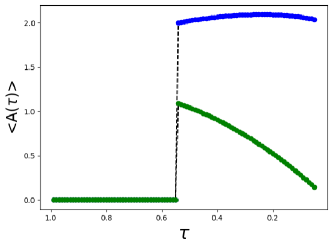
Figure 4: Average amplitude with decreasing $\tau$ for $\epsilon=3$. The tipping from IHSS state to synchronized oscillations is seen in layer L1(blue) and layer L2(green), as the $\tau$ is varied. The other parameter values are: $K_{1}=K_{2}=10$, $P_{1}=1$, $P_{2}=25$, $\omega=2$ and $\gamma=1$

Figure 5: Schematic representation of the three-layer network, where nodes in the middle layer (L2) (blue) illustrate the environment while nodes in the upper (L1) and lower (L3) layers (orange) represent the system layers.

3 Three layer system

The study is extended to a three layer multiplex system with the L1 and L3 layers as networks of $N$ SL oscillators and the environment in the middle layer L2 as shown in the Fig. 5. The equations for the dynamics of the three layer system are presented below.

$$\dot{x}_{i1} = (1-x_{i1}^{2}-y_{i1}^{2})x_{i1}-\omega y_{i1}+\frac{K_{1}}{2P_{1}}\sum_{j=i-P_{1}}^{i+P_{1}}(x_{j1}-x_{i1})+\epsilon_{1}s_{i2}$$

$$\dot{y}_{i1} = (1-x_{i1}^{2}-y_{i1}^{2})y_{i1}+\omega x_{i1}$$

$$\dot{s}_{i2} = \tau[-\gamma s_{i2}-\epsilon_{1}x_{i1}-\epsilon_{2}x_{i3}+\frac{K_{2}}{2P_{2}}\sum_{j=i-P_{2}}^{i+P_{2}}(s_{j2}-s_{i2})]$$

$$\dot{x}_{i3} = (1-x_{i3}^{2}-y_{i3}^{2})x_{i3}-\omega y_{i3}+\frac{K_{3}}{2P_{3}}\sum_{j=i-P_{3}}^{i+P_{3}}(x_{j3}-x_{i3})+\epsilon_{2}s_{i2}$$

$$\dot{y}_{i3} = (1-x_{i3}^{2}-y_{i3}^{2})y_{i3}+\omega x_{i3}$$

Figure 6: Time series of the x-variable of Stuart-Landau oscillators (L1-red, L3-green) and s-variable of the environment (blue). (a): Anti synchronization between L1 and L3 for $\epsilon_{1}=\epsilon_{2}=2.5$ and $\tau=1$, (b): Complete synchronization between L1 and L3 for $\epsilon_{1}=\epsilon_{2}=2.5$ and $\tau=0.1$. The other parameter values are: $K_{1}=K_{2}=K_{3}=15$, $P_{1}=P_{3}=1$, $P_{2}=25$, $\omega=2$ and $\gamma=1$

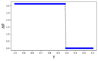
Figure 7: Variation in the phase difference $\Delta\theta$ between L1 and L3 as $\tau$ is varied for $\epsilon_{1}=\epsilon_{2}=2.5$. The other parameter values are: $K_{1}=K_{2}=K_{3}=15$, $P_{1}=P_{3}=1$, $P_{2}=25$, $\omega=2$ and $\gamma=1$

where the SL oscillators are characterized by the variables $x_{ik}$ and $y_{ik}$ for i = 1, 2, …, N in the $k^{th}$ layer, where $k=1,3$. In addition, $\epsilon_{1}$ and $\epsilon_{2}$ represent the inter-layer coupling strength for L1 and L3, respectively. All other parameters are consistent with those previously described in the two-layer scenario.

Figure 8: Spatio temporal plots from the $y_{i}$ variable of Stuart-Landau oscillators in L1 for the three-layer multiplex network. (a): Inhomogeneous steady state for $\epsilon_{1}=\epsilon_{2}=5$ and $\tau=1$, (b): Synchronized oscillations for $\epsilon_{1}=\epsilon_{2}=5$ and $\tau=0.1$. The other parameter values are: $P_{1}=P_{3}=1$, $P_{2}=40$, $K_{1}=K_{3}=30$, $K_{2}=1$, $\omega=2$ and $\gamma=1$

Similar to the two-layer case, we consider all SL oscillators in L1 and L3 connected with one another locally, with $P_{1}=P_{3}=1$ and the environment L2 is coupled nonlocally, with $P_{2}=25$. We show that it is possible to revive synchronized oscillations from different dynamical states by tuning the parameter $\tau$ in the three layer system also.

When there is no time scale mismatch between the layers, for random initial conditions we observe synchronized oscillations in the system layers, with L1 and L3 being anti synchronized to each other for parameter values of $K_{1}=K_{2}=K_{3}=15$, $\gamma=1$, $\omega=2$ and $\epsilon_{1}=\epsilon_{2}=2.5$ as shown in Fig. 6(a). In this case, the environment goes to death due to the cancelling feedback from the system layer. As time scale mismatch is introduced, the layers L1 and L2 go from anti synchronization to perfect synchronization, as shown in Fig. 6(b) with the revival of oscillations in L2 also. In Fig. 7 we show this transition by plotting the phase difference $\Delta\theta$ between L1 and L3, with varying $\tau$.

A similar recovery of synchronized oscillations is observed from IHSS also. For parameter values of $P_{1}=P_{3}=1$, $P_{2}=40$, $K_{1}=K_{3}=30$, $K_{2}=1$, $\gamma=1$ and $\omega=2$ the system shows IHSS for $\epsilon_{1}=\epsilon_{2}=5$ and $\tau=1$ as shown in Fig. 8(a) from which synchronized oscillations are revived as depicted in Fig. 8(b) for $\tau=0.1$

4 Conclusion

In this letter, we report the revival of synchronized oscillations in a multiplex network by tuning the time scale separation between the layers of the system. We first consider a two-layer network where the first layer consists of an ensemble of SL oscillators, while the second layer model the environment. When both layers evolve with the same time scale, the coupled system exhibits various emergent phenomena, such as amplitude chimera, chimera death, HSS, IHSS, and 2-CSS. By tuning the time scale difference between the layers, we show the synchronized oscillations can be restored in both layers from these different states. By computing the measures, strength of incoherence and average amplitude, we characterise the possible dynamical states and show the nature of their transitions to synchronized oscillations. The revival of synchronized oscillations are also shown with van der Pol oscillators and chaotic Rössler systems on layer L1.

We also consider a three layer multiplex network, with the upper and lower layers as coupled SL oscillators, and the middle layer as environment. For identical time scale and lower value of interlayer coupling, first layer’s oscillators are exactly in anti-phase with third layer oscillators. When mismatch is time scale is introduced between the environment and system layers, the system layers go to complete synchronization. Similarly for identical time scale but higher value of interlayer coupling , the system shows inhomogeneous steady state from which synchronized oscillations are revived by introducing time scale difference between layers.

We note the present study has relevance in controlling systems evolving under differing time scales to desired synchronized oscillations like in neuronal networks, power grids, climate and ecosystems. In eco systems, the time scale difference between intrinsic dynamics and environmental changes is shown to have a decisive role in inducing transitions in the system [60]. The role of a slowly changing environment is studied by introducing a drift in the relevant parameters. In our study we include environment as a layer multiplexed with the system layer. This gives more flexibility to track the impact of slowly varying environment and also to arrive at control mechanisms to achieve desired emergent states even in the presence of heterogeneity among interacting systems.

References

- [1] D.J. Watts, S.H. Strogatz, Nature 393 ( 1998) 440-2.
- [2] M. D. Domenico, A. Solé-Ribalta, E. Cozzo, M. Kivelä, Y. Moreno, M. A. Porter, S. Gómez A. Arenas, Phys. Rev. X 3 (2013) 41022.
- [3] M Kivelä , A Arenas, M Barthelemy, J.P Gleeson, Y Moreno, M.A Porter, J. Complex. Netw. 2 (2013) 203-71.
- [4] U.K Verma, G Ambika, Chaos 30 (2020).
- [5] S Boccaletti, V Latora, Y Moreno, Handbook on Biological Networks, World Scientific Lectures Notes in Complex Systems, vol. 10, 2009.
- [6] M Sadilek, S Thurner, Sci. Rep. 5 (2014).
- [7] P Deville, C Song, N Eagle, V.D Blondel, A Barabási, D Wang, Proc. Natl.Acad. Sci. 113 (2016) 7047-52.
- [8] G.A Pagani, M Aiello, Physica A 392 (2013) 2688-700.
- [9] S Makovkin, T Laptyeva, S Jalan, M Ivanchenko, Chaos 31 (2021).
- [10] X Wei, J Zhao, S Liu, Y Wang, Sci. Rep. 12 (2022) 5550.
- [11] S Strogatz, Phys. Today 56 (2003) 56:47.
- [12] L.M Pecora LM, F Sorrentino, A.M Hagerstrom, T.E Murphy, R Roy, Nat. Commun. 5 (2014) 4079.
- [13] G Saxena, A Prasad, R Ramaswamy, Phys. Rep. 521 (2012) 205-28.
- [14] A Koseska, E Volkov, J Kurths, Phys. Rev. Lett. 111 (2013) 024103.
- [15] S Pranesh, S Gupta, Chaos Solitons and Fractals 168 (2023) 113112.
- [16] L Smirnov, G Osipov, A Pikovsky, J. Phys. A Math. Theor. 50 (2017).
- [17] E Schöll, Europhys. Lett. 136 (2021) 18001.
- [18] E Schöll, Eur. Phys. J. Spec. Top 225 (2016) 891-919.
- [19] I.A Shepelev, T.E Vadivasova, Phys. Lett. A 382 (2015) 690-96.
- [20] S.A Bogomolov, A.V Slepnev, G.I Strelkova, E Schöll, V.S Anishchenko, Commun. Nonlin. Sci. Numer. Simul. 43 (2017) 25-36.
- [21] A Zakharova, S Loos, J Siebert, A Gjurchinovski, E Schöll, IFAC-PapersOnLine 48 (2015) 7-12.
- [22] J Sawicki, S Ghosh, S Jalan, A Zakharova. Front. Appl. Math. Stat. 5 (2019) 19.
- [23] S Kachhara, G Ambika, Phys. Rev. E 104 (2021) 064214.
- [24] A Rothkegel, K Lehnertz, New J. Phys. 16 (2014) 055006.
- [25] N.C Rattenborg, C.J Amlaner, S.L Lima, Neurosci. Biobehav. Rev. 24 (2000) 817-42.
- [26] S Deng, G Ódor, Chaos 34 (2024).
- [27] G.C Sethia, A Sen, Phys. Rev. Lett. 112 (2014) 144101.
- [28] S Ghosh, S Jalan, Int. J. Bifurcat. Chaos. 26 (2015).
- [29] D.M Abrams, R Mirollo, S.H Strogatz, D.A Wiley. Phys. Rev. Lett. 101 (2008) 084103.
- [30] A Zakharova, M Kapeller, E Schöll E, Phys. Rev. Lett. 112 (2014) 154101.
- [31] T Banerjee, Europhys. Lett. 110 (2015) 60003.
- [32] I Omelchenko, T Hulser, A Zakharova, E Schöll, Front. Appl. Math. Stat. 4 (2019) 67.
- [33] V.A Maksimenko, V.V Makarov, B.K Bera, D Ghosh, S.K Dana, M.V Goremyko, N.S Frolov, A.A Koronovskii, A.E Hramov, Phys. Rev. E 94 (2016) 052205.
- [34] S Majhi, M Perc, D Ghosh, Chaos 27 (2017).
- [35] J Sawicki, I Omelchenko, A Zakharova, E Schöll, Eur. Phys. J. Spec. Top 227 (2018) 1161-71.
- [36] N Semenova, A Zakharova, Chaos 28 (2018) 51104.
- [37] J Sawicki, J.M Koulen, E Schöll, Chaos 31 (2021).
- [38] X Mao, X Li, W Ding, S Wang, X Zhou, L Qiao, Appl. Math. Mech. 42 (2021).
- [39] M.S Anwar, S Rakshit, J Kurths, D Ghosh Entropy 25 (2023) 1083.
- [40] U.K Verma, G Ambika, Phys. Lett. A 450 (2022) 128391.
- [41] T Wu, S Huo, K Alfaro-Bittner, S Boccaletti, Z Liu, Phys. Rev. Res. 4 (2022) 33009.
- [42] V Nicosia, P.S Skardal, A Arenas, V Latora, Phy. Rev. Lett. 118 (2017) 138302.
- [43] D Kasatkin, V Nekorkin, Chaos 28 (2018) 93115.
- [44] A Sharma, M Shrimali, K Aihara, Phys. Rev. E 2014;90:62907.
- [45] I Levya, I Sendiña-Nadal, R Sevilla-Escoboza, V.P Vera-Avila, P Chholak, S Boccaletti, Sci. Rep. 8 (2018) 8629.
- [46] A.E Motter, S.A Myers, M Anghel, T Nishikawa, Nat. Phys. 9 (2013) 191-97.
- [47] P Fries, J.H Reynolds, A.E Rorie, R Desimone, Science 291 (2001) 1560-63.
- [48] A Jenkins, Phys. Rep. 525 (2013) 167-222.
- [49] W Samek, D.A.J Blythe, G Curio, K.R Müller, B Blankertz, V.V Nikulin, NeuroImage 141 (2016) 291-303.
- [50] E.S Boyden, F Zhang, E Bamberg, G Nagel, K Deisseroth, Nat. Neurosci. 8 (2005) 1263-68.
- [51] A.G Gilman, J. Clin. Investig 73 (1984) 1-4.
- [52] S Radovick, M Nations, Y Du, L.A Berg, B.D Weintraub, F.E Wondisford, Science 257 (1992) 1115-18.
- [53] D Das, D.S Ray, Eur. Phys. J. Spec. Top 222 (2013) 785-98.
- [54] R Schiestel, Phys. Fluids 30 (1987) 722-731.
- [55] I Bena, M Droz, J Szwabiński, A Pȩkalski, Phys. Rev. E 76 (2007) 011908.
- [56] K Gupta, G Ambika, Chaos 29 (2019).
- [57] S Jalan, A Singh, Europhys. Lett. 113 (2016) 30002.
- [58] W Yang, Y Wang, Y Shen, L Pan, Nonlin. Dyn. 90 (2017) 2767-82.
- [59] R Gopal, V.K Chandrasekar, A Venkatesan, M Lakshmanan, Phys. Rev. E 89 (2014) 052914.
- [60] U Feudel, Nonlin. Processes Geophys. 30 (2023) 481-502