Comparison of 4.5PN and 2SF gravitational energy fluxes
from quasicircular compact binaries

Abstract

The past three years have seen two significant advances in models of gravitational waveforms emitted by quasicircular compact binaries in two regimes: the weak-field, post-Newtonian regime, in which the gravitational wave energy flux has now been calculated to fourth-and-a-half post-Newtonian order (4.5PN) [Phys. Rev. Lett. 131, 121402 (2023)]; and the small-mass-ratio, gravitational self-force regime, in which the flux has now been calculated to second perturbative order in the mass ratio (2SF) [Phys. Rev. Lett. 127, 151102 (2021)]. We compare these results and find excellent agreement for the total flux, showing consistency between the two calculations at all available PN and SF orders. However, although the total fluxes agree, we find disagreements in the fluxes due to individual spherical-harmonic modes of the waveform, strongly suggesting the two waveforms might be in different asymptotic frames.

I Introduction

Future gravitational-wave (GW) detectors will demand improved waveform models, both due to improved instrument sensitivity and due to a larger variety of systems that will be observed [1, 2]. This has motivated continual progress in modeling the waveform emission from binary systems of black holes and neutron stars [3].

Recently, two important milestones were achieved in this effort, specifically in perturbation methods for general relativity (GR) applied to gravitational waves from compact binary systems on quasicircular orbits: (i) the gravitational self-force (GSF) approach was pushed to second order in the small mass ratio, both for the binary’s conserved mass-energy [4] and the GW emission [5, 6]; (ii) the post-Newtonian (PN) approximation was completed at the 4PN order for the equations of motion [7, 8, 9, 10, 11, 12] and at the 4.5PN order (beyond the Einstein quadrupole formula) for the energy flux [13, 14, 15, 16, 17, 18, 19], while the dominant $(\ell,m)=(2,2)$ mode was obtained at 4PN order [18, 19]. The aim of this paper is to compare the salient results of the two approaches, confirming the preliminary agreement found in [20].

For the purposes of the comparison, we focus on a binary system of two nonspinning black holes of masses $m_{1}$ and $m_{2}$ on a bound orbit. We assume that there is no incoming radiation and that the spacetime is asymptotically flat. By convention, we assume $m_{1}\geqslant m_{2}$ (and $m_{1}\gg m_{2}$ in the GSF case); we denote the total mass $m_{\mathrm{tot}}=m_{1}+m_{2}$ and the symmetric mass ratio $\nu=m_{1}m_{2}/m_{\mathrm{tot}}^{2}$. Far away from the binary, we assume a linearized metric around Minkowski, $g_{\alpha\beta}=\eta_{\alpha\beta}+h_{\alpha\beta}$, and introduce a spherical coordinate system $(u,r,\theta,\phi)$ such that $u$ is a null coordinate (i.e., $g^{uu}=0$). We will also use the usual spherical harmonics $Y^{\ell m}(\theta,\phi)$ as well as the spin-weighted ones $Y_{-2}^{\ell m}(\theta,\phi)$, where the integer $m$ should not be confused with a mass. We often set $G=c=1$ and pose $\mathcal{O}(n)\equiv\mathcal{O}(c^{-n})$ for small PN remainders.

We write the asymptotic gravitational wave in a transverse traceless (TT) gauge, and decompose it into a “plus” mode $h_{+}$ and a “cross” mode $h_{\times}$. We can then expand the waveform $h\equiv h_{+}-\mathrm{i}h_{\times}$ into spin-weighted spherical harmonics (with weight $-2$) as follows:

$$h =\frac{1}{r}\sum_{\ell=2}^{+\infty}\sum_{m=-\ell}^{\ell}h_{\ell m}(u)\,Y_{-2}^{\ell m}(\theta,\phi)+\mathcal{O}\!\left(\frac{1}{r^{2}}\right)\,,$$ (1)

where $h$ is dimensionless and $h_{\ell m}$ has dimension of length since we have factored out the dependence on the radial distance in order to state purely asymptotic results. Each mode can be factorized as

$$h_{\ell m}(u)=m_{\mathrm{tot}}\,\hat{h}_{\ell m}(u)\,\mathrm{e}^{-\mathrm{i}m\psi(u)}\,,$$ (2)

where the $\hat{h}_{\ell m}$ are dimensionless and we choose by convention that $\hat{h}_{22}$ is real-valued. Thus, the imaginary parts of the other $\hat{h}_{\ell m}$ modes account for higher-order dephasing between the different modes. We define the dimensionless parameter

$$x\equiv\bigl{(}m_{\mathrm{tot}}\,\omega\bigr{)}^{2/3}\,,$$ (3)

which is related to the frequency $\omega\equiv\mathrm{d}\psi/\mathrm{d}u$ associated to the $(2,2)$ mode and represents the small PN parameter $x=\mathcal{O}(2)$.

In the case of quasicircular orbits to which we will now specialize, the time dependence of $\hat{h}_{\ell m}$ is entirely captured by $x(u)$ and $\nu(u)$, namely we can write $\hat{h}_{\ell m}\equiv\hat{h}_{\ell m}(x,\nu)$. The frequency variable $x$ and masses $m_{i}$ evolve secularly, following equations of the form

$$\frac{\mathrm{d}x}{\mathrm{d}u} =\frac{\Xi(x,\nu)}{m_{\mathrm{tot}}}\,,$$ (4a)

$$\frac{\mathrm{d}m_{i}}{\mathrm{d}u} ={\cal F}_{\mathcal{H}_{i}}(x,\nu)\,,$$ (4b)

where ${\cal F}_{\mathcal{H}_{i}}(x,\nu)$ is the flux of energy into the horizon of the black hole of mass $m_{i}$. Here $\hat{h}_{\ell m}$, $\Xi$, and ${\cal F}_{\mathcal{H}_{i}}$ are dimensionless and therefore can only be functions of dimensionless combinations of the binary’s frequency $\omega$ and masses $m_{i}$ — and all such combinations can be written in terms of $x$ and $\nu$. Equations (4) allow us to apply the chain rule

$$\frac{\mathrm{d}}{\mathrm{d}u}=\frac{\Xi(x,\nu)}{m_{\mathrm{tot}}}\,\frac{\partial}{\partial x}+\sum_{i=1,2}{\cal F}_{\mathcal{H}_{i}}(x,\nu)\,\frac{\partial}{\partial m_{i}}\,,$$ (5)

when acting on $h_{\ell m}$ with derivatives of $u$. The asymptotic energy flux carried by GWs reads

$$\mathcal{F}=\frac{1}{16\pi}\int\mathrm{d}\Omega_{2}\,|\dot{h}|^{2}=\sum_{\ell=2}^{+\infty}\sum_{m=1}^{\ell}\mathcal{F}_{\ell m}(x,\nu)\,,$$ (6)

where the dot stands for $\mathrm{d}/\mathrm{d}u$ and where we have defined

$$\mathcal{F}_{\ell m}(x,\nu)=\frac{1}{8\pi}|\dot{h}_{\ell m}|^{2}\,.$$ (7)

Note that $m=0$ modes do not contribute for quasicircular orbits at the orders we consider, and a factor of 2 has appeared when expressing the sum in terms of positive $m$ modes, due to the relationship $h_{\ell(-m)}=(-)^{m}{h}_{\ell m}^{*}$ (the star $*$ indicates complex conjugation). Also note that although $\dot{h}_{\ell m}$ is a function of $(x,\nu,\psi)$, the modulus squared $|\dot{h}_{\ell m}|^{2}$ depends only on $(x,\nu)$.

These fluxes are related in a one-to-one manner to the moduli of the $h_{\ell m}$ modes, but do not carry any information about the phases. In the PN approach, which assumes small orbital frequencies, we obtain the fluxes as an expansion in the small parameter $x$ of Eq. (3), with coefficients that are functions of $\nu$:

$$\mathcal{F}_{\ell m}(x,\nu)=\frac{32}{5}\,\nu^{2}x^{5}\biggl{[}1+\!\!\sum_{q\geqslant 2,\,k\geqslant 0}\!\!\mathcal{F}^{qk}_{\ell m}(\nu)\,x^{q/2}(\ln x)^{k}\biggr{]}\,.$$ (8)

Conversely, the self-force approach assumes small mass ratios and obtains the flux as an expansion in $\nu$, with coefficients that are functions of $x$:

$$\mathcal{F}_{\ell m}(x,\nu)=\nu^{2}\biggl{[}\mathcal{F}^{(1)}_{\ell m}(x)+\nu\mathcal{F}^{(2)}_{\ell m}(x)+{\cal O}(\nu^{2})\biggr{]}\,,$$ (9)

where the SF order “$(n)$” indicates the order in $\nu$ at which the field equations are solved in order to obtain the corresponding flux contribution $\mathcal{F}^{(n)}_{\ell m}$.

To compare the two expansions of the flux, we note that formally, one can perform a double expansion in $x$ and $\nu$, so as to obtain an expression of the form

$$\mathcal{F}_{\ell m}=\frac{32}{5}\,\nu^{2}x^{5}\!\!\!\!\!\sum_{p\geqslant 0,\,q\geqslant 0,\,k\geqslant 0}\!\!\!\mathcal{F}^{pqk}_{\ell m}\nu^{p}x^{q/2}(\ln x)^{k}\,.$$ (10)

As both the PN and GSF methods are first-principle perturbation methods of GR, they should yield strictly the same coefficients $\mathcal{F}^{pqk}_{\ell m}$ in the expansion (this statement still holds when applied to each individual $\mathcal{F}_{\ell m}$). The 4.5PN expression [18] and the 1SF results of analytical black hole perturbation [21, 22] theory have been shown to agree [18], namely the coefficients $\mathcal{F}^{pqk}_{\ell m}$ for $p=0$ and $q\in[\![0,9]\!]$ are strictly identical. Reference [5] additionally showed numerical agreement between the flux at 2SF and 3.5PN.

The goal of this article is to confirm the agreement up to 4.5PN. Our central conclusion is that the 2SF and 4.5PN results agree on the total flux at each available order: i.e. $\sum_{\ell m}\mathcal{F}^{pqk}_{\ell m}$ agrees between the two methods for $p=1$ and $q\in[\![0,9]\!]$ (and $k=0$ or $1$). However, we also find a notable disagreement on the individual mode contributions $\mathcal{F}^{pqk}_{\ell m}$ beyond 3.5PN order, which precisely cancels in the sum over modes. As we discuss below, this might indicate that the PN and GSF waveforms are calculated in different asymptotic frames.

II Review of 4.5PN flux

The 4.5PN flux and waveform of compact binaries have been obtained by combining two approximation methods: the classic PN expansion which assumes small orbital velocities ($v/c\to 0$), equivalent to large separations between the two bodies, and the multipolar post-Minkowskian (MPM) method which combines the PM or non-linearity expansion ($G\to 0$) with multipolar series parametrized by specific multipole moments. The PN expansion is implemented in an inner domain (or near zone) covering the matter source but whose radius is much less than a gravitational wavelength. The MPM expansion is valid in an external domain which overlaps with the near zone of the source and extends into the far wave zone. The MPM field represents the most general solution of the Einstein field equation (say, in harmonic coordinates) in the exterior zone. The PN and MPM expansions are matched in the exterior part of the near zone, which is the region of common validity of both expansions: the whole procedure is called the post-Newtonian-multipolar-post-Minkowkian (PN-MPM) formalism [23, 24, 25, 26, 27].

The MPM construction of the metric is carried out as a functional of a set of parameters, called the “canonical” mass and current type multipole moments $\mathrm{M}_{L}(t)$ and $\mathrm{S}_{L}(t)$, which are symmetric and trace-free (STF) with respect to their $\ell$ indices (where $L\equiv i_{1}\cdots i_{\ell}$). The canonical moments are defined from the linearized approximation $\mathfrak{h}^{\alpha\beta}_{1}[\mathrm{M}_{L},\mathrm{S}_{L}]$ of the MPM construction,

$$\mathfrak{h}^{\alpha\beta}_{\text{MPM}}=\sum_{n=1}^{+\infty}G^{n}\,\mathfrak{h}^{\alpha\beta}_{n}[\mathrm{M}_{L},\mathrm{S}_{L}]\,,$$ (11)

where $\mathfrak{h}^{\alpha\beta}=\sqrt{-g}g^{\alpha\beta}-\eta^{\alpha\beta}$ is the “gothic metric deviation”, and each PM approximation is computed iteratively [23]. The time dependence of the metric includes many non-local integrals over the moments $\mathrm{M}_{L}$, $\mathrm{S}_{L}$, from $t=-\infty$ up to the current time. The matching to the PN field in the source’s near zone determines the relations between $\mathrm{M}_{L}$, $\mathrm{S}_{L}$ and the actual “source” mass and current multipole moments $\mathrm{I}_{L}$, $\mathrm{J}_{L}$, say

$$\mathrm{M}_{L}=\mathrm{I}_{L}+\mathcal{O}(5)\,,\qquad\mathrm{S}_{L}=\mathrm{J}_{L}+\mathcal{O}(5)\,,$$ (12)

where the PN remainder terms are entirely controlled with the 4PN precision [28, 19]. Here $\mathrm{I}_{L}$, $\mathrm{J}_{L}$ are functionals of the matter plus gravitation pseudo stress-energy tensor $\overline{\tau}^{\alpha\beta}$ (the overbar means the PN expansion),

$$\mathrm{I}_{L}=\mathop{\mathrm{FP}}_{B=0}\int\mathrm{d}^{d}\mathbf{x}\,\Bigl{(}\frac{r}{r_{0}}\Bigr{)}^{B}\hat{x}_{L}\bigl{[}\overline{\tau}^{00}+\overline{\tau}^{ii}\bigr{]}+\cdots\,,$$ (13)

where $\hat{x}_{L}$ is the STF projection of $x_{L}=x_{i_{1}}...x_{i_{\ell}}$, the finite part (FP) denotes a particular IR regularization when $B\to 0$ depending on an arbitrary regularization scale $r_{0}$, and the ellipsis denote other terms, known to all orders for general systems.

Once the external MPM metric is determined, we expand it to leading order in the distance between source and observer, to obtain the asymptotic waveform and the GW observables at infinity. Because harmonic coordinates asymptotically exhibit logarithms of the radial coordinate, which spoil the multipolar structure of the asymptotic waveform, we introduce a (non harmonic) “radiative” coordinate system adapted to the fall-off of the metric at infinity. By radiative coordinate system we mean one such that the retarded time $u=t-r$ is a null (or asymptotically null) coordinate, thus avoiding the logarithmic deviation of the retarded time in harmonic coordinates with respect to the true light cone. Alternatively, a different MPM construction defined in [24], corrects the coordinate light-cones at every PM order so as to iteratively build the null coordinate $u$, with the far zone logarithms therefore automatically cancelled. This construction has played a crucial role in our calculation of the 4PN flux.

The transverse-traceless (TT) waveform can be uniquely decomposed into two sets of STF “radiative” multipole moments $\mathrm{U}_{L}$, $\mathrm{V}_{L}$, which encode all the information about the asymptotic metric. These moments can straightforwardly be expressed in terms of the spherical harmonic modes as in Eq. (1), see (2.5)–(2.7) of [29]. The MPM construction determines (in principle up to any order) their relation to the canonical moments. For instance the leading term is the well-known nonlocal quadrupole tail integral arising at the 1.5PN order,

$$\mathrm{U}_{ij}(u)=\mathrm{M}^{(2)}_{ij}(u)+2\mathrm{M}\int_{-\infty}^{u}\mathrm{d}\tau\,\mathrm{M}^{(4)}_{ij}(\tau)$$

$$\qquad\qquad\qquad\times\left[\ln\left(\frac{u-\tau}{b_{0}}\right)+\frac{11}{12}\right]+\mathcal{O}(5)\,,$$ (14)

where $\mathrm{M}$ is the monopole of the multipole expansion (i.e. the Arnowitt-Deser-Misner mass of the spacetime) and $b_{0}$ is an arbitrary constant length scale linked to the definition of radiative coordinates. Beyond the tail term in (II), one finds the nonlinear memory effect at orders 2.5PN and 3.5PN; the tail-of-tail at 3PN order (a cubic interaction between two masses $\mathrm{M}$ and the time-varying quadrupole); the tails-of-memory at 4PN order, which is a cubic interaction between $\mathrm{M}$ and two varying quadrupoles [17]; the spin quadrupole tail at 4PN order (interaction $\mathrm{M}\times\mathrm{S}_{i}\times\mathrm{M}_{L}$); and at 4.5PN order the quartic tail-of-tail-of-tail interation, composed of three masses $\mathrm{M}$ and the quadruole [14].

The PN-MPM formalism is applied to compact binary sources. The compact objects are modeled by point particles (we neglect spins and other finite size effects). Furthermore, in a first stage of the calculation the two masses $m_{i}$ are considered to be constant, i.e. we neglect the black hole absorption, which should be added separately at the end of the PN calculation.

The first manifestation of BH absorption is that the individual masses $m_{i}$ evolve according to (4b). We know that the horizon flux ${\cal F}_{\mathcal{H}_{i}}$ for nonspinning BHs is comparable to a 4PN orbital effect (beyond the 2.5PN Einstein quadrupole formula). For circular orbits it reads

$${\cal F}_{\mathcal{H}_{i}}=\frac{32}{5}\,\Bigl{(}\frac{m_{i}}{m_{\mathrm{tot}}}\Bigr{)}^{2}x^{5}\Bigl{[}\kappa\,x^{4}+\mathcal{O}(x^{5})\Bigr{]}\,,$$ (15)

where $x$ is the orbital frequency (3) and $\kappa=1$ has been computed in the test mass limit in Ref. [30]. By integrating Eqs. (4b)–(15) using the dominant radiation reaction effect on the orbit ($\dot{x}\propto x^{5}$) one finds

$$m_{i}=\bar{m}_{i}+\frac{\kappa}{10}m_{\mathrm{tot}}\nu\,x^{5}+\mathcal{O}(x^{6})\,,$$ (16)

where $\bar{m}_{i}$ denotes the initial mass before the GW emission (say, when $x\to 0$). Thus the evolution of the mass by BH absorption is comparable to a very small 5PN orbital effect. We can ignore this effect and consider the masses to be constant in our 4.5PN calculation. The second impact of BH absorption is that the energy flux balance law is modified as

$$\frac{\mathrm{d}E}{\mathrm{d}t}=-\mathcal{F}-\sum_{i=1,2}\mathcal{F}_{\mathcal{H}_{i}}\,,$$ (17)

where ${\cal F}$ denotes the energy flux at infinity. Therefore, when solving Eq. (17) to obtain the expression of the frequency evolution (or chirp), i.e. $\dot{x}$ expressed in terms of $x$, we shall obtain extra 4PN corrections due to the horizon fluxes. Those will affect the equations of motion at 4PN order beyond the dominant 2.5PN radiation reaction, i.e. corresponding to 6.5PN radiation reaction terms. When obtaining the 4.5PN flux at infinity, Eq. (II) below, we only required the expression of the frequency chirp at 1.5PN order beyond the dominant order (see (5.3b) of [19]), hence the above 6.5PN radiation reaction terms can be safely discarded in our calculation. Our conclusion is that the BH absorption plays no role in the derivation of the energy flux at infinity (II) at this order, so we shall directly compare it with the GSF result in Sec. IV.

The equations of motion of the compact binary system have already been obtained at 4PN order [7, 8, 9, 10, 11, 12] and we extensively use the result. The most important task is the computation of the source multipole moments $\mathrm{I}_{L}$, $\mathrm{J}_{L}$ for the binary source, see Eq. (13). The source moments represent the seed of the full construction through the steps (12)–(II). The 4PN mass quadrupole moment $\mathrm{I}_{ij}$ has been obtained in [13, 15, 16]. Previous works had determined that UV divergences, due to the modelling of compact objects by point masses, appear at the 3PN order and require the use of dimensional regularization. After regularization a shift of the particle’s world lines permits to absorb the divergences. The works [13, 15, 16] showed that at the 4PN order IR divergences appear as well. For reasons explained in [9, 10], we have used a variant of dimensional regularization called the “$B\epsilon$” regularization, where the finite part at $B=0$ in Eq. (13) is applied on the top of the calculation performed in $d=3+\epsilon$ dimensions. An important point is that the regularization constant $r_{0}$ in (13) is finally cancelled in the radiative moment (II), due notably to the $r_{0}$ dependence of the tails-of-memory. Besides the 4PN mass quadrupole moment, we also need the 3PN mass octupole $\mathrm{I}_{ijk}$ and 3PN current quadrupole $\mathrm{J}_{ij}$, which have been obtained in [31] and [32], respectively.

It is known that the GW half-phase $\psi$, defined by the decomposition of Eq. (2), and the orbital phase $\phi$, which is used in the computation to parameterize the circular motion of the binary, differ by a logarithmic phase modulation at order 1.5PN, which is due to the propagation of tails in the wave zone [33, 34, 35],

$$\psi\equiv\phi-2\mathrm{M}\ln\left(\frac{\omega}{\omega_{0}}\right)+\mathcal{O}(5)\,.$$ (18)

The constant $\omega_{0}$ is related to the constant $b_{0}$ in (II) by $\omega_{0}^{-1}=4b_{0}\,\mathrm{e}^{\gamma_{\text{E}}-11/12}$ (where $\gamma_{\text{E}}$ is the Euler constant). While the GW phase $\psi$ and the corresponding frequency $\omega=\mathrm{d}\psi/\mathrm{d}u$ are directly measurable, the orbital phase $\phi$ can only be inferred via the theoretical prediction (18).

Taking the time derivative of Eq. (18), and using the fact that the time evolution of the phase occurs on a 2.5PN radiation reaction time scale, we find that the orbital frequency $\omega_{\text{orb}}=\mathrm{d}\phi/\mathrm{d}u$ and GW frequency $\omega=\mathrm{d}\psi/\mathrm{d}u$ differ by a small 4PN term, which thus enters for the first time in the 4PN waveform. A consequence is that the frequency parameter $x$ defined by (3) differs from its counterpart $y=(m_{\text{tot}}\,\omega_{\text{orb}})^{2/3}$ by a small 4PN correction:

$$x=y\,\biggl{\{}1-\frac{192}{5}\,\nu\,y^{4}\biggl{[}\ln\biggl{(}\frac{y}{y_{0}}\biggr{)}+\frac{2}{3}\biggr{]}+\mathcal{O}(y^{5})\biggr{\}}\,,$$ (19)

where $y_{0}=(m_{\text{tot}}\,\omega_{0})^{2/3}$ and $\mathcal{O}(y^{5})=\mathcal{O}(10)$. When expressing physical results in terms of the GW observables $\psi$ and $\omega$, the arbitrary scale $b_{0}$ is canceled out (see [19] for details).

Another subtlety that arises at 4PN order is the treatment of the tail integral (II). To compute it explicitly at 3.5PN order for a quasicircular orbit, it is sufficient to assume that the orbital frequency and orbit radius are constant — this is the “adiabatic” approximation. However this approximation is no longer valid at relative 2.5PN precision, because this is the order of radiation reaction; one must then consistently account for the time evolution of the orbital frequency as well. Since the tail term enters at the 1.5PN order, the first “post-adiabatic” correction will affect the waveform at the 4PN order, and it needs to be properly evaluated in order to control the 4PN flux and modes [19].

The end result for the dominant mode $(\ell,m)=(2,2)$ at 4PN order, following the definition (1)–(2), reads

$$\hat{h}_{22}=\sqrt{\frac{64\pi}{5}}\,\nu x\bigg{\{}1+\Bigl{(}-\tfrac{107}{42}+\tfrac{55}{42}\nu\Bigr{)}x+2\pi x^{3/2}$$

$$+\Bigl{(}-\tfrac{2173}{1512}-\tfrac{1069}{216}\nu+\tfrac{2047}{1512}\nu^{2}\Bigr{)}x^{2}+\Bigl{(}-\tfrac{107}{21}+\tfrac{34}{21}\nu\Bigr{)}\pi x^{5/2}$$

$$+\biggl{[}\tfrac{27027409}{646800}-\tfrac{856}{105}\,\gamma_{\text{E}}+\tfrac{2\pi^{2}}{3}+\Bigl{(}-\tfrac{278185}{33264}+\tfrac{41\pi^{2}}{96}\Bigr{)}\nu$$

$$\qquad-\tfrac{20261}{2772}\nu^{2}+\tfrac{114635}{99792}\nu^{3}-\tfrac{428}{105}\ln(16x)\biggr{]}x^{3}$$

$$+\Bigl{(}-\tfrac{2173}{756}-\tfrac{2495}{378}\nu+\tfrac{40}{27}\nu^{2}\Bigr{)}\pi x^{7/2}$$

$$+\biggl{[}-\tfrac{846557506853}{12713500800}+\tfrac{45796}{2205}\gamma_{\text{E}}-\tfrac{107}{63}\pi^{2}+\tfrac{22898}{2205}\ln(16x)$$

$$+\Bigl{(}-\tfrac{336005827477}{4237833600}+\tfrac{15284}{441}\gamma_{\text{E}}-\tfrac{9755}{32256}\pi^{2}+\tfrac{7642}{441}\ln(16x)\Bigr{)}\nu$$

$$+\Bigl{(}\tfrac{256450291}{7413120}-\tfrac{1025}{1008}\pi^{2}\Bigr{)}\nu^{2}-\tfrac{81579187}{15567552}\nu^{3}+\tfrac{26251249}{31135104}\nu^{4}\biggr{]}x^{4}$$

$$+\mathcal{O}(x^{9/2})\bigg{\}}\,.$$ (20)

Unlike in previous works, e.g. [18, 19], we have chosen the convention that the amplitude of the (2,2) mode be real valued. The amplitude given in Eq. (II) is thus equal (up to a global prefactor) to the modulus of the amplitude given by Eq. (11) of [18]. This difference of course leads to corrections to the phase evolution $\psi(u)$, but these are very small 5PN modulations beyond the leading order in the phase (which is $\propto x^{-5/2}$), for instance comparable to neglected terms in Eq. (19). The result (II) is in perfect agreement with linear black-hole perturbation theory at first order (i.e. 1SF) in the mass ratio [21, 22]. For the other modes up to 3.5PN order, we refer to Refs. [29, 36].

Finally, adding up all pieces together we obtain the quasi-circular 4.5PN flux [18, 19]

$$\mathcal{F}=\frac{32}{5}\nu^{2}x^{5}\biggl{\{}1+\Bigl{(}-\tfrac{1247}{336}-\tfrac{35}{12}\nu\Bigr{)}x+4\pi x^{3/2}$$

$$+\Bigl{(}-\tfrac{44711}{9072}+\tfrac{9271}{504}\nu+\tfrac{65}{18}\nu^{2}\Bigr{)}x^{2}+\Bigl{(}-\tfrac{8191}{672}-\tfrac{583}{24}\nu\Bigr{)}\pi x^{5/2}$$

$$+\biggl{[}\tfrac{6643739519}{69854400}+\tfrac{16}{3}\pi^{2}-\tfrac{1712}{105}\gamma_{\text{E}}-\tfrac{856}{105}\ln(16\,x)$$

$$~{}~{}+\Bigl{(}-\tfrac{134543}{7776}+\tfrac{41}{48}\pi^{2}\Bigr{)}\nu-\tfrac{94403}{3024}\nu^{2}-\tfrac{775}{324}\nu^{3}\biggr{]}x^{3}$$

$$+\Bigl{(}-\tfrac{16285}{504}+\tfrac{214745}{1728}\nu+\tfrac{193385}{3024}\nu^{2}\Bigr{)}\pi x^{7/2}$$

$$+\biggl{[}-\tfrac{323105549467}{3178375200}+\tfrac{232597}{4410}\gamma_{\text{E}}-\tfrac{1369}{126}\pi^{2}$$

$$~{}~{}+\tfrac{39931}{294}\ln 2-\tfrac{47385}{1568}\ln 3+\tfrac{232597}{8820}\ln x$$

$$~{}~{}+\Bigl{(}-\tfrac{1452202403629}{1466942400}+\tfrac{41478}{245}\gamma_{\text{E}}-\tfrac{267127}{4608}\pi^{2}$$

$$\quad\quad+\tfrac{479062}{2205}\ln 2+\tfrac{47385}{392}\ln 3+\tfrac{20739}{245}\ln x\Bigr{)}\nu$$

$$~{}~{}+\Bigl{(}\tfrac{1607125}{6804}-\tfrac{3157}{384}\pi^{2}\Bigr{)}\nu^{2}+\tfrac{6875}{504}\nu^{3}+\tfrac{5}{6}\nu^{4}\biggr{]}x^{4}$$

$$+\biggl{[}\tfrac{265978667519}{745113600}-\tfrac{6848}{105}\gamma_{\text{E}}-\tfrac{3424}{105}\ln(16\,x)$$

$$~{}~{}+\Bigl{(}\tfrac{2062241}{22176}+\tfrac{41}{12}\pi^{2}\Bigr{)}\nu-\tfrac{133112905}{290304}\nu^{2}-\tfrac{3719141}{38016}\nu^{3}\biggr{]}\pi x^{9/2}$$

$$+\mathcal{O}(x^{5})\biggr{\}}\,.$$ (21)

The decomposition of the total flux into mode contributions $\mathcal{F}_{\ell\textrm{m}}$ is relegated to Appendix A.

III Review of 2SF fluxes

In the GSF formulation of the binary problem, the primary object is taken to be a black hole, the secondary object is reduced to a point particle, and the spacetime metric is expanded in powers of the binary’s mass ratio.

We denote the zeroth-order, background metric as $\mathring{g}_{\alpha\beta}(x^{i})$, representing the spacetime of the primary black hole in isolation, meaning a Schwarzschild geometry with constant mass $\mathring{m}_{1}$. The variables $x^{i}=(r/\mathring{m}_{1},\theta,\phi)$ are the usual Schwarzschild spatial coordinates, adimensionalized with the background mass $\mathring{m}_{1}$. We define the mass ratio $\varepsilon$ in terms of this background mass as $\varepsilon\equiv m_{2}/\mathring{m}_{1}$.

The first- and second-order corrections to $\mathring{g}_{\alpha\beta}$, due to the orbiting particle, are obtained using a multiscale formulation of the expansion in $\varepsilon$, detailed in Refs. [37, 38]. In this approach, powers of $\varepsilon$ represent post-adiabatic (PA) orders [39, 40]; the leading (0PA) order is the traditional adiabatic approximation, in which the system adiabatically evolves through a smooth sequence of test-particle orbits. Concretely, our multiscale approach assumes the spacetime’s evolution arises entirely from the evolution of the binary’s mechanical variables $(\phi_{p},\Omega,\delta m_{1})$, where $\phi_{p}$ is the particle’s orbital (azimuthal) phase,

$$\Omega\equiv\mathring{m}_{1}\frac{\mathrm{d}\phi_{p}}{\mathrm{d}t}$$ (22)

is its (adimensionalized) slowly evolving orbital frequency, and

$$\delta m_{1}\equiv(m_{1}-\mathring{m}_{1})/m_{2}$$ (23)

is an adimensionalized correction to the black hole’s mass parameter, which evolves due to the black hole’s absorption of radiation. The mass evolves by an amount of order $m_{2}$ over the course of the inspiral, and we adimensionalize $\delta m_{1}$ using $m_{2}$ to make it order unity. The mass $m_{2}$, on the other hand, is constant at 2SF order.

In terms of these mechanical variables and the spatial coordinates $x^{i}$, the metric is expanded as

$$g_{\alpha\beta}=\mathring{g}_{\alpha\beta}(x^{i})+\varepsilon h^{(1)}_{\alpha\beta}(\phi_{p},\Omega,\delta m_{1},x^{i})\\ +\varepsilon^{2}h^{(2)}_{\alpha\beta}(\phi_{p},\Omega,\delta m_{1},x^{i})+{\cal O}(\varepsilon^{3})\,.$$ (24)

Because the mass only changes by an amount $\sim m_{2}$ over the inspiral time $\sim 1/\varepsilon$, the evolving correction is treated perturbatively rather than altering $\mathring{g}_{\alpha\beta}$. No explicit dependence on a time coordinate appears in the metric (24) because time dependence is subsumed into the dependence on $(\phi_{p},\Omega,\delta m_{1})$.

As described in Refs. [37, 38], the mechanical variables are treated as functions of a hyperboloidal time coordinate $s$ that reduces to Schwarzschild time $t$ on the particle, retarded Eddington-Finkelstein time $u$ at future null infinity, and advanced Eddington-Finkelstein time $v$ at the horizon, adimensionalized by $\mathring{m}_{1}$. Their time evolution (and hence, the spacetime’s evolution) is governed by equations of the form

$$\frac{\mathrm{d}\phi_{p}}{\mathrm{d}s} =\Omega\,,$$ (25a)

$$\frac{\mathrm{d}\Omega}{\mathrm{d}s} =\varepsilon\Bigl{[}F_{0}^{\Omega}(\Omega)+\varepsilon F_{1}^{\Omega}(\Omega,\delta m_{1})+{\cal O}(\varepsilon^{2})\Bigr{]}\,,$$ (25b)

$$\frac{\mathrm{d}\delta m_{1}}{\mathrm{d}s} =\varepsilon\mathcal{F}^{(1)}_{{\cal H}_{1}}(\Omega)+{\cal O}(\varepsilon^{2})\,.$$ (25c)

Here $\mathcal{F}^{(1)}_{{\cal H}_{1}}$ is the standard energy flux carried by $h^{(1)}_{\alpha\beta}$ across the primary’s event horizon [41]. The forcing function $F_{0}^{\Omega}(\Omega)$ is the standard adiabatic (0PA) rate of change of the orbital frequency, which is related to the emitted energy flux by

$$F_{0}^{\Omega}=-\frac{\mathcal{F}^{(1)}+\mathcal{F}^{(1)}_{{\cal H}_{1}}}{\mathrm{d}{\cal E}_{0}/\mathrm{d}\Omega}\,,$$ (26)

where $\mathcal{F}^{(1)}$ is the standard energy flux carried by $h^{(1)}_{\alpha\beta}$ to future null infinity [41], and ${\cal E}_{0}$ is the specific orbital energy of a test mass on a circular geodesic with frequency $\Omega$. This forcing function $F_{0}^{\Omega}$ enters the Einstein field equations for $h^{(2)}_{\alpha\beta}$ and into explicit expressions for the 2SF flux below; the first post-adiabatic (1PA) forcing function $F_{1}^{\Omega}$, on the other hand, does not enter into the calculation of the 2SF fluxes. Note that here we have factored out powers of $\varepsilon$ such that $F_{n}^{\Omega}$, ${\cal F}^{(1)}_{{\cal H}_{1}}$, ${\cal F}^{(1)}$, and ${\cal E}_{0}$ are all $\varepsilon$-independent functions of $\Omega$.

The waveform in the multiscale expansion, in analogy with Eq. (24), takes the form

$$h_{\ell m}=\mathring{m}_{1}\left[\varepsilon h^{(1)}_{\ell m}(\Omega)+\varepsilon^{2}h^{(2)}_{\ell m}(\Omega,\delta m_{1})+{\cal O}(\varepsilon^{3})\right]\mathrm{e}^{-\mathrm{i}m\phi_{p}}\,,$$ (27)

where $h^{(n)}_{\ell m}$ is obtained from the coefficient of $1/r$ in the large-$r$ limit of the metric perturbation $h^{(n)}_{\alpha\beta}$ in a Bondi-Sachs (radiative) gauge [42]. In practice, we solve the Einstein equations for $h^{(n)}_{\alpha\beta}$ in the Lorenz gauge, which is not well behaved at large $r$ [43, 37, 38] (as in the PN case in Sec. II), and then transform to a Bondi-Sachs gauge to eliminate the ill-behaved pieces of the Lorenz-gauge solution.

It is possible to obtain the flux directly from the waveform (27). Explicitly, substituting Eq. (27) into the flux formula (7), one finds

$$\mathcal{F}_{\ell m} =\frac{1}{8\pi}\biggl{\{}\varepsilon^{2}\bigl{|}m\Omega\,h^{(1)}_{\ell m}\bigr{|}^{2}+2\varepsilon^{3}\,\Re\left(m^{2}\Omega^{2}h^{(2)}_{\ell m}h^{(1)*}_{\ell m}\right.$$

$$\qquad\qquad\left.+\mathrm{i}m\Omega\,F^{\Omega}_{0}\,h^{(1)*}_{\ell m}\partial_{\Omega}h^{(1)}_{\ell m}\right)+{\cal O}(\varepsilon^{4})\biggr{\}}\,.$$ (28)

To recast this in a form suitable for comparison with the PN flux, we can re-express it in terms of the common variables $(x,m_{\mathrm{tot}},\nu)$ and re-expand in powers of $\nu$ at fixed $(x,m_{\mathrm{tot}})$.

However, before proceeding to the flux, it will be instructive to instead re-express the waveform itself in terms of the shared variables. This will provide a more intuitive link between the waveform and the flux. We start by expressing the waveform in terms of $(m_{\mathrm{tot}},\nu)$ and an orbital frequency parameter (as opposed to the waveform frequency). The various masses are related by

$$\mathring{m}_{1} =m_{1}-m_{2}\delta m_{1}\,,$$ (29a)

$$m_{1} =\frac{m_{\mathrm{tot}}}{2}\bigl{(}1+\sqrt{1-4\nu}\bigr{)}\,,$$ (29b)

$$m_{2} =\frac{m_{\mathrm{tot}}}{2}\bigl{(}1-\sqrt{1-4\nu}\bigr{)}\,.$$ (29c)

Re-expanding (27) in powers of $\nu$ at fixed $m_{\mathrm{tot}}$ leads to

$$h_{\ell m}=m_{\mathrm{tot}}\left[\nu\tilde{h}^{(1)}_{\ell m}(y)+\nu^{2}\tilde{h}^{(2)}_{\ell m}(y)+{\cal O}(\nu^{3})\right]\mathrm{e}^{-\mathrm{i}m\phi_{p}}\,,$$ (30)

where

$$\tilde{h}^{(1)}_{\ell m}(y) =h^{(1)}_{\ell m}(y^{3/2})\,,$$ (31a)

$$\tilde{h}^{(2)}_{\ell m}(y) =h^{(2)}_{\ell m}(y^{3/2},\delta m_{1})+h^{(1)}_{\ell m}(y^{3/2})$$

$$\quad-(1+\delta m_{1})y^{3/2}\partial_{\Omega}h^{(1)}_{\ell m}(y^{3/2})\,.$$ (31b)

Here $y$ is the parameter introduced above Eq. (19); it is related to our dimensionless $\Omega$ by

$$y=\left(\frac{m_{\mathrm{tot}}}{\mathring{m}_{1}}\Omega\right)^{2/3}\,.$$ (32)

Note that the dependence on $\delta m_{1}$ cancels on the right-hand side of Eq. (31b), leaving only a dependence on the frequency variable $y$.

To express the waveform in terms of the waveform frequency, we go one step further by writing the waveform (30) in terms of a real amplitude and complex phase factor,

$$h_{\ell m}=m_{\mathrm{tot}}A_{\ell m}\mathrm{e}^{-\mathrm{i}m\psi_{\ell m}}\,,$$ (33)

where $A_{\ell m}=|h_{\ell m}|/m_{\mathrm{tot}}$ and $m\psi_{\ell m}=-\arg(h_{\ell m})$. This corresponds to Eq. (2) with the identifications $\psi=\psi_{22}$ and $A_{\ell m}=|\hat{h}_{\ell m}|$. Substituting Eq. (30), we then find the analogue of the PN phase modulation (18):

$$m\psi_{\ell m} =m\phi_{p}-\nu^{0}\arg\bigl{(}\tilde{h}^{(1)}_{\ell m}\bigr{)}$$

$$+\nu\,\frac{\Re\,\tilde{h}^{(2)}_{\ell m}\,\Im\,\tilde{h}^{(1)}_{\ell m}-\Im\,\tilde{h}^{(2)}_{\ell m}\,\Re\,\tilde{h}^{(1)}_{\ell m}}{\bigl{|}\tilde{h}^{(1)}_{\ell m}\bigr{|}^{2}}+{\cal O}(\nu^{2})\,.$$ (34)

We can assess the importance of each term on the right-hand side by noting that the phases $\psi_{\ell m}$ and $\phi_{p}$ are both ${\cal O}(\nu^{-1})$ quantities; on the radiation-reaction timescale $m_{\mathrm{tot}}/\nu$, the phases evolve by an amount of order $1/\nu$. Hence the order-$\nu^{0}$ term in Eq. (III) represents a relative 1PA phase correction, while the order-$\nu$ term represents a relative 2PA phase correction. Likewise, the order-$\nu$ term will only affect the waveform frequency at 2PA order ($\sim~{}\nu^{2}$) because it only involves the slowly evolving quantities ($y,m_{\mathrm{tot}},\nu$), with no direct dependence on $\phi_{p}$. Hence, we only require the first two terms in Eq. (III).

Finally, we relate the waveform frequency to the orbital frequency by applying a time derivative to Eq. (III) and using (25b) together with $\mathrm{d}\nu/\mathrm{d}u=\mathcal{O}(\nu^{3})$. This yields the result previously presented in Ref. [44] (generalized to generic $\ell m$),

$$\dot{\psi}_{\ell m}\equiv\omega_{\ell m}=\dot{\phi}_{p}+\nu\omega^{(1)}_{\ell m}+\mathcal{O}(\nu^{2})\,,$$ (35)

with

$$m\omega^{(1)}_{\ell m}=\frac{2F^{\Omega}_{0}}{3y^{1/2}\bigl{|}\tilde{h}^{(1)}_{\ell m}\bigr{|}^{2}}\left({\Im}\,\tilde{h}^{(1)}_{\ell m}\,{\Re}\,\partial_{y}\tilde{h}^{(1)}_{\ell m}-{\Re}\,\tilde{h}^{(1)}_{\ell m}\,{\Im}\,\partial_{y}\tilde{h}^{(1)}_{\ell m}\right)\!.$$ (36)

Following the general discussion in the Introduction, we define the waveform frequency as $\omega=\omega_{22}$. The analogue of the PN equation (19) then reads

$$x=y\left[1+\frac{2m_{\mathrm{tot}}\omega^{(1)}}{3y^{3/2}}\nu+{\cal O}(\nu^{2})\right]\,,$$ (37)

with $\omega^{(1)}\equiv\omega^{(1)}_{22}$. We can also express the general $\omega_{\ell m}$ as a function of $\omega$:

$$\omega_{\ell m}=\omega+\nu\Delta\omega^{(1)}_{\ell m}+{\cal O}(\nu^{2})\,,$$ (38)

where $\Delta\omega^{(1)}_{\ell m}\equiv\omega^{(1)}_{\ell m}-\omega^{(1)}$.

Substituting Eq. (37) into Eq. (30), we obtain $h_{\ell m}$ in terms of the waveform frequency:

$$h_{\ell m}=m_{\mathrm{tot}}\Bigl{[}\nu A^{(1)}_{\ell m}(x)+\nu^{2}A^{(2)}_{\ell m}(x)+{\cal O}(\nu^{3})\Bigr{]}\mathrm{e}^{-\mathrm{i}m\psi_{\ell m}}\,,$$ (39)

where

$$A^{(1)}_{\ell m} =\bigl{|}\tilde{h}^{(1)}_{\ell m}\bigr{|}\,,$$ (40a)

$$A^{(2)}_{\ell m} =\frac{1}{2\bigl{|}\tilde{h}^{(1)}_{\ell m}\bigr{|}}\biggl{[}\tilde{h}^{(1)*}_{\ell m}\biggl{(}\tilde{h}^{(2)}_{\ell m}-\frac{2m_{\mathrm{tot}}\omega^{(1)}}{3x^{1/2}}\partial_{x}\tilde{h}^{(1)}_{\ell m}\biggr{)}+\text{c.c.}\biggr{]}\,.$$ (40b)

Functions of $y$ or $\Omega$ on the right side are evaluated at $x$ or $x^{3/2}$, respectively.

In terms of the real amplitudes $A_{\ell m}$, the flux (7) takes a simple form,

$${\cal F}_{\ell m} =\frac{m_{\mathrm{tot}}^{2}}{8\pi}\biggl{[}m^{2}\omega_{\ell m}^{2}(A_{\ell m})^{2}+\left(\frac{\mathrm{d}x}{\mathrm{d}u}\right)^{\!\!2}(\partial_{x}A_{\ell m})^{2}+\mathcal{O}(\nu^{4})\biggr{]}$$

$$=\frac{m^{2}m_{\mathrm{tot}}^{2}\omega_{\ell m}^{2}}{8\pi}(A_{\ell m})^{2}+{\cal O}(\nu^{4})\,,$$ (41)

where we have used $A_{\ell m}=\mathcal{O}(\nu)$ together with $d\nu/du=\mathcal{O}(\nu^{3})$ and $\mathrm{d}m_{1}/\mathrm{d}u=\mathcal{O}(\nu^{2})$ to neglect time derivatives of $\nu$ and $m_{\mathrm{tot}}$ in the first line, and $\mathrm{d}x/\mathrm{d}u=\mathcal{O}(\nu)$ in the second line. After substituting the expansions of $A_{\ell m}$ and $\omega_{\ell m}$, we can rewrite this in the form (9):

$${\cal F}_{\ell m}=\frac{\nu^{2}m^{2}m_{\mathrm{tot}}^{2}}{8\pi}\biggl{\{}\omega^{2}\bigl{(}A^{(1)}_{\ell m}\bigr{)}^{2}+2\nu\Bigl{[}\omega^{2}A^{(1)}_{\ell m}A^{(2)}_{\ell m}\\ +\omega\Delta\omega^{(1)}_{\ell m}\bigl{(}A^{(1)}_{\ell m}\bigr{)}^{2}\Bigr{]}+{\cal O}(\nu^{2})\biggr{\}}\,.$$ (42)

IV Comparison

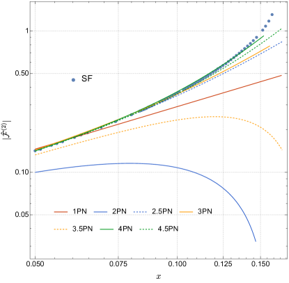
Figure 1: Comparison between GSF and PN for the 2SF $\mathcal{O}(\nu)$ contribution to the (Newtonian-normalized) total flux (43). The 2SF results are shown with (blue) dots. The PN results are shown with coloured curves with integer PN orders shown with solid curves and corresponding half-integer orders shown with dashed curves.

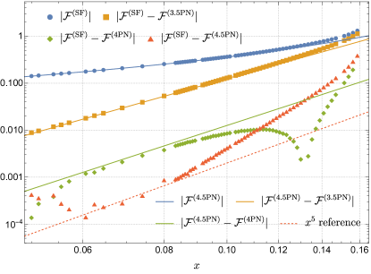
Figure 2: Detailed comparison between the $\mathcal{O}(\nu)$ PN and GSF results for the (Newtonian-normalized) total flux. The 2SF data are shown by (blue) dots and the PN series are plotted with solid curves. As ever higher-order PN series are subtracted from the GSF results the residual at small $x$ behaves as expected. After subtracting the 3.5PN series from the GSF data, one gets the (yellow) squares which follow the $\mathcal{O}(x^{4})$ behaviour of the 4PN series (yellow curve). Subtracting the 4PN series from the SF data, one gets the (green) diamonds. This agrees with the $\mathcal{O}(x^{9/2})$ term in the 4.5PN series (green curve) though for $x\lesssim 0.06$ the numerical error in the GSF calculation dominates the comparison. After subtracting all known terms in the PN series there is evidence that the residual has the expected $x^{5}$ behaviour (dashed, red line).

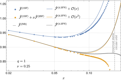
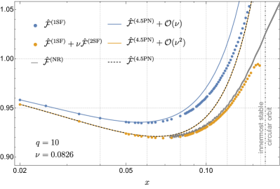
Figure 3: (Left Panel) Comparison between the (Newtonian-normalized) GSF and PN total flux at different orders in the mass ratio expansion for $q=1$ ($\nu=0.25$). It is interesting to note that the 4.5PN expansion, including all orders in $\nu$ (black, dashed curve), is closely approximated by the expansion truncated at $\mathcal{O}(\nu^{2})$ (yellow, solid curve). In gray we also show the flux computed from an NR simulation by the SXS collaboration [45], specifically SXS:BBH:1132 [46]. The shaded width of the gray curve is an estimate on the numerical error in the simulation. (Right Panel) The same as the left panel but for $q=10$ ($\nu=0.0826$). The NR simulation in this plot is SXS:BBH:1107 [47].

We present the results of our extensive comparison between the numerical 2SF data and the analytic 4.5PN flux given by Eq. (II). In computing the total 2SF flux, we sum the $(\ell,m)$ modes up to $\ell=7$. We find that the contribution from modes with higher $\ell$ does not affect the comparison. For the purpose of the GSF and PN comparison, we define the Newtonian-normalized flux as

$$\hat{\mathcal{F}}\equiv\frac{\mathcal{F}}{\mathcal{F}_{\rm N}}\,,\qquad\hat{\mathcal{F}}_{\ell m}\equiv\frac{\mathcal{F}_{\ell m}}{\mathcal{F}_{\rm N}}\,,$$ (43)

where the Newtonian flux reads

$$\mathcal{F}_{\rm N}=\frac{32}{5}\nu^{2}x^{5}\,.$$ (44)

In Fig. 1 we plot the GSF data at 2SF order, i.e. corresponding to the $\mathcal{O}(\nu)$ terms in the normalized flux (43), together with the PN predictions at various orders up to 4.5PN. We nicely find that both the 4PN and 4.5PN are very close to the 2SF prediction, say until the relativistic regime at around $x\sim 0.15$. Previous PN approximations do clearly less well. While 3PN is still rather good, the half-integer (odd-parity) 3.5PN is off. By contrast, 2.5PN is surprisingly close to the 2SF result, while the even-parity 2PN is the worst approximation in the series. We also note that 1PN does relatively well. Here the PN expansion is in Taylor-expanded form, without resummation techniques applied.

Figure 2 goes further in the comparison by checking that the PN behaviour of the flux is indeed contained in and reproduced by the 2SF result for various orders. Observe in particular the residual obtained after subtraction of all known PN terms from the 2SF result. The residual is consistent with the expected 5PN behaviour $\mathcal{O}(x^{5})$ of the systematic PN error. For small values of $x$ the non-smoothness of the residual after subtracting the 4PN and 4.5PN results stems from numerical error in the GSF calculation. The level of this noise is consistent with the error in each $(\ell,m)$ being similar to the estimated error in the (2,2) mode as shown in Fig. 7 of [5].

Although Fig. 2 provides convincing evidence that the 2SF and 4.5PN results agree for the total Newtonian-normalized flux $\hat{\mathcal{F}}$, we also find compelling evidence that the individual mode contributions $\hat{\mathcal{{F}}}_{\ell m}$ do not agree beyond 3.5PN order. We explore that comparison in Appendix A. This disagreement at the level of individual mode contributions, which cancels when the contributions are summed, might indicate that the GSF and PN waveforms are computed in different asymptotic Bondi-Metzner-Sachs (BMS) frames [48].

In Fig. 3 we assess the accuracy and convergence of the SF fluxes when benchmarked against PN and numerical relativity (NR); this complements the analogous assessment of PN in Fig. 1. Here we include the normalized total flux at 1SF [i.e., neglecting $\mathcal{O}(\nu)$] and 2SF [neglecting $\mathcal{O}(\nu^{2})$] alongside 4.5PN and NR results for two mass ratios: $q=1$ (left panel) and $q=10$ (right panel). We see that for both mass ratios, the 2SF flux provides a marked improvement over the 1SF result. The SF expansion, moving from 1SF to 2SF, converges well toward the NR result, achieving nice agreement with NR for the large mass ratio $q=10$ throughout the strong field regime $x\gtrsim 0.07$ where the NR data is available. The SF expansion also converges nicely toward the PN result in the weak field, with the PN and 2SF results agreeing extremely well in the mildly relativistic regime, say $x\lesssim 0.07$, for both mass ratios. To further illustrate the convergence, we also include curves for the 4.5PN flux truncated at 1SF and at 2SF. The latter agrees extremely well with the full 4.5PN flux for all values of $x$, showing that higher-order corrections $\mathcal{O}(\nu^{2})$ are numerically small even at $q=1$. We note that for $q=1$, the 4.5PN flux remains more accurate than the 2SF flux, when measured against NR, even in the strong field up to $x\sim 0.1$ (a very relativistic value by PN standards). Figure 3 thus illustrates the importance of synergies between the PN, SF, and NR approaches to cover the whole range of scenarios of compact binary coalescences.

V Conclusion

We have compared the results of two significant recent advances in perturbative techniques for GWs emitted by compact binary systems, focusing on the energy flux for quasicircular orbits: on the one hand, the analytical slow-motion weak-field post-Newtonian approximation, pushed to 4.5PN order beyond the Einstein quadrupole formula [18, 19]; on the other hand, the numerical gravitational self-force approach developed to second order in the small mass ratio limit [5, 6].

Previous comparisons of the 4.5PN quasicircular flux were performed using the GSF flux to first order in the mass ratio. To 1SF level the GSF results can be derived analytically to high order in the PN expansion [21, 22, 49, 50], and the PN coefficients are perfectly consistent up to 4.5PN order with direct PN calculations valid for arbitrary mass ratios. Note that at 1SF/0PA order, the flux at infinity for quasicircular inspirals is identical to the flux generated by a particle on a fixed background geodesic.

The new comparisons at the 2SF level reported in this paper are numerical, building on the earlier comparisons with the 3.5PN flux in Ref. [5]. The 2SF fluxes take into account the contribution coming from the 1SF deviation in the motion of the particle generating the GW and flux at infinity, as well as quadratic nonlinearities in waveform generation and propagation. As shown in Figs. 1, 2, and 3, the agreement with the PN coefficients for the total flux is excellent.

A key aspect of our analysis is that invariant comparisons require precise knowledge of how the orbital frequency relates to the waveform frequency. Agreement between the 4.5PN and 2SF fluxes is only achieved when the fluxes are computed as functions of an invariant waveform frequency, eliminating the gauge/slicing dependence of the relationship between the orbit and the waveform.

Another interesting outcome of our comparison is that while the total PN and SF fluxes agree through 4.5PN order, they disagree at the level of individual spherical-harmonic mode contributions beyond 3.5PN order. This is highly suggestive of the two waveforms being in different BMS frames. Future work will explore the choice of frame in the 2SF waveform and determine whether mode-by-mode agreement with PN can be achieved through a frame transformation, as has been done in numerical relativity [51].

VI Acknowledgments

N.W. acknowledges support from a Royal Society – Science Foundation Ireland University Research Fellowship. This publication has emanated from research conducted with the financial support of Science Foundation Ireland under grant number 22/RS-URF-R/3825. D.T. received support from the Czech Academy of Sciences under the grant number LQ100102101. A.P. acknowledges the support of a Royal Society University Research Fellowship and the UKRI Frontier Research Grant GWModels, as selected by the ERC and funded by UKRI under the Horizon Europe Guarantee scheme [grant number EP/Y008251/1].

Appendix A Comparison of individual mode contributions to the flux

The comparisons in the body of the paper are for the total flux to infinity, summed over $(\ell,m)$ mode contributions. However, additional information about the PN and SF waveform amplitudes can be gleaned by comparing the individual $(\ell,m)$ contributions.

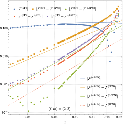
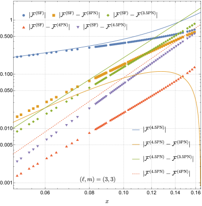
Figure 4: (Left panel) Comparison between $\mathcal{O}(\nu)$ GSF and PN results for the (Newtonian-normalized) fluxes for the (2,2) mode. At the level of individual modes we do not see agreement after 3.5PN. (Right panel) Same as the left panel but for the (3,3) mode. The PN results for the (2,2) and (3,3) modes are respectively given by (47a) and (47c).

At 4PN order, the modes can be straightforwardly obtained by inserting the $(2,2)$ mode amplitude (II) and Eqs. (3.4) of [36] for the other modes, into Eq. (7). Moreover, we can extend this result at 4.5PN order with the sole knowledge of the hereditary part of the first time derivative of the radiative moments [14]. Using (2.6)–(2.7) of [29] it comes

$$\mathcal{F}_{\ell m} =\frac{1}{16\pi}\Bigl{[}|\dot{\mathrm{U}}_{\ell m}|^{2}+|\dot{\mathrm{V}}_{\ell m}|^{2}\Bigr{]}\,,$$ (45)

where

$$\mathrm{U}_{\ell m} =\frac{4}{\ell!}\,\sqrt{\tfrac{(\ell+1)(\ell+2)}{2\ell(\ell-1)}}\,\alpha_{L}^{\ell m}\,\mathrm{U}_{L}\,,$$ (46a)

$$\mathrm{V}_{\ell m} =-\frac{8}{\ell!}\,\sqrt{\tfrac{\ell(\ell+2)}{2(\ell+1)(\ell-1)}}\,\alpha_{L}^{\ell m}\,\mathrm{V}_{L}\,.$$ (46b)

We have defined the STF tensorial coefficient $\alpha_{L}^{\ell m}=\int\mathrm{d}\Omega_{2}\,\hat{n}_{L}(\theta,\phi){Y}_{\ell m}^{*}(\theta,\phi)$, see e.g. (4.7) of [32] for an explicit expression.

The explicit 4.5PN expressions of the decomposition of the total flux are given in Eq. (47) hereafter; we have verified that these expressions agree perfectly with Eqs. (A.3-27) of [22] at first order in the mass ratio. We present the results in terms of the normalized fluxes $\hat{\mathcal{F}}_{\ell m}$ defined in Eq. (43).

Finally we present in Figs. 4 the comparison between the 2SF and PN results for the flux contributions from the individual spherical-harmonic modes (2,2) and (3,3). We find that the individual modes do not agree well beyond 3.5PN order, even though the sum of the modes agrees as we have seen in Fig. 2. This disagreement on the separate modes may be due to the fact that the GSF waveform has been computed in an asymptotic frame different from that of the PN waveform.

A difference in asymptotic frame would not be surprising. Historically, little work has been done to control the BMS frame in GSF calculations, which have mostly used intuition from the Newtonian-order analysis in Ref. [52]. A BMS transformation, whether an ordinary Poincaré transformation or a supertranslation, can significantly alter the individual $(\ell,m)$ modes of the waveform [48, 51], and this freedom remains unexplored in GSF calculations. An analysis of this freedom, and whether it can resolve the mode-by-mode discrepancy we find, is left for future work.

$$\hat{\mathcal{F}}_{22} =1+\left(-\frac{107}{21}+\frac{55}{21}\nu\right)x+4\pi x^{3/2}+\left(\frac{4784}{1323}-\frac{87691}{5292}\nu+\frac{5851}{1323}\nu^{2}\right)x^{2}+\left(-\frac{428}{21}+\frac{178}{21}\nu\right)\pi x^{5/2}$$

$$\ \ \,\quad+\left(\frac{99210071}{1091475}-\frac{1712}{105}\gamma_{E}+\frac{16}{3}\pi^{2}-\frac{856}{105}\ln(16x)+\nu\left[\frac{1650941}{349272}+\frac{41}{48}\pi^{2}\right]-\frac{669017}{19404}\nu^{2}+\frac{255110}{43659}\nu^{3}\right)x^{3}$$

$$\ \ \,\quad+\left(\frac{19136}{1323}-\frac{144449}{2646}\nu+\frac{33389}{2646}\nu^{2}\right)\pi x^{7/2}$$

$$\ \ \,\quad+\Bigg{(}-\frac{27956920577}{81265275}+\frac{183184}{2205}\gamma_{\mathrm{E}}-\frac{1712}{63}\pi^{2}+\frac{91592}{2205}\ln(16x)$$

$$\ \ \,\quad\qquad+\nu\left[\frac{440671815511}{57210753600}+\frac{21152}{441}\gamma_{\mathrm{E}}+\frac{87757}{16128}\pi^{2}+\frac{10576}{441}\ln(16x)\right]$$

$$\ \ \,\quad\qquad+\nu^{2}\left[\frac{488191373}{4643730}-\frac{205}{224}\pi^{2}\right]-\frac{249670210}{5108103}\nu^{3}+\frac{4763492}{729729}\nu^{4}\Bigg{)}x^{4}$$

$$\ \ \,\quad+\Bigg{(}\frac{396840284}{1091475}-\frac{6848}{105}\gamma_{\mathrm{E}}-\frac{3424}{105}\ln(16x)+\nu\left[\frac{1882981}{174636}+\frac{41}{12}\pi^{2}\right]-\frac{885179}{8316}\nu^{2}+\frac{2627879}{174636}\nu^{3}\Bigg{)}\pi x^{9/2}+\mathcal{O}(x^{5})$$ (47a)

$$\hat{\mathcal{F}}_{21} =\left(\frac{1}{36}-\frac{\nu}{9}\right)x+\left(-\frac{17}{504}+\frac{11}{63}\nu-\frac{10}{63}\nu^{2}\right)x^{2}+\left(\frac{1}{18}-\frac{2}{9}\nu\right)\pi x^{5/2}$$

$$\quad+\left(-\frac{2215}{254016}-\frac{13567}{63504}\nu+\frac{65687}{63504}\nu^{2}-\frac{853}{5292}\nu^{3}\right)x^{3}+\left(-\frac{17}{252}+\frac{9}{28}\nu-\frac{13}{63}\nu^{2}\right)\pi x^{7/2}$$

$$\quad+\Bigg{(}\frac{15707221}{26195400}-\frac{107}{945}\gamma_{\mathrm{E}}+\frac{\pi^{2}}{27}-\frac{107}{1890}\ln(4x)+\nu\left[-\frac{17451737}{3742200}+\frac{428}{945}\gamma_{\mathrm{E}}-\frac{409}{6912}\pi^{2}+\frac{214}{945}\ln(4x)\right]$$

$$\ \ \,\quad\quad+\nu^{2}\left[\frac{74234059}{8382528}-\frac{205}{576}\pi^{2}\right]+\frac{965}{1134}\nu^{3}-\frac{70787}{523908}\nu^{4}\Bigg{)}x^{4}$$

$$\quad+\Bigg{(}-\frac{2215}{127008}-\frac{23669}{63504}\nu+\frac{115141}{63504}\nu^{2}-\frac{305}{1764}\nu^{3}\Bigg{)}\pi x^{9/2}+\mathcal{O}(x^{5})$$ (47b)

$$\hat{\mathcal{F}}_{33} =\left(\frac{1215}{896}-\frac{1215}{224}\nu\right)x+\left(-\frac{1215}{112}+\frac{10935}{224}\nu-\frac{1215}{56}\nu^{2}\right)x^{2}+\left(\frac{3645}{448}-\frac{3645}{112}\nu\right)\pi x^{5/2}$$

$$\quad+\left(\frac{243729}{9856}-\frac{92907}{616}\nu+\frac{2171691}{9856}\nu^{2}-\frac{17901}{352}\nu^{3}\right)x^{3}+\left(-\frac{3645}{56}+\frac{258795}{896}\nu-\frac{3645}{32}\nu^{2}\right)\pi x^{7/2}$$

$$\quad+\Bigg{(}\frac{25037019729}{125565440}-\frac{47385}{1568}\gamma_{\mathrm{E}}+\frac{3645}{224}\pi^{2}-\frac{47385}{3136}\ln(36x)$$

$$\qquad\quad+\nu\left[-\frac{84912893811}{125565440}+\frac{47385}{392}\gamma_{\mathrm{E}}-\frac{1816425}{28672}\pi^{2}+\frac{47385}{784}\ln(36x)\right]$$

$$\qquad\quad+\nu^{2}\left[-\frac{45782091}{73216}-\frac{49815}{7168}\pi^{2}\right]+\frac{149211477}{256256}\nu^{3}-\frac{5737635}{64064}\nu^{4}\Bigg{)}x^{4}$$

$$\quad+\Bigg{(}\frac{731187}{4928}-\frac{34272963}{39424}\nu+\frac{45879129}{39424}\nu^{2}-\frac{2379213}{9856}\nu^{3}\Bigg{)}\pi x^{9/2}+\mathcal{O}(x^{5})$$ (47c)

$$\hat{\mathcal{F}}_{32} =\left(\frac{5}{63}-\frac{10}{21}\nu+\frac{5}{7}\nu^{2}\right)x^{2}+\left(-\frac{193}{567}+\frac{1304}{567}\nu-\frac{2540}{567}\nu^{2}+\frac{365}{189}\nu^{3}\right)x^{3}+\left(\frac{20}{63}-\frac{40}{21}\nu+\frac{20}{7}\nu^{2}\right)\pi x^{7/2}$$

$$\quad+\Bigg{(}\frac{86111}{280665}-\frac{183244}{56133}\nu+\frac{709004}{56133}\nu^{2}-\frac{4009259}{224532}\nu^{3}+\frac{181429}{56133}\nu^{4}\Bigg{)}x^{4}$$

$$\quad+\Bigg{(}-\frac{772}{567}+\frac{5126}{567}\nu-\frac{9620}{567}\nu^{2}+\frac{170}{27}\nu^{3}\Bigg{)}\pi x^{9/2}+\mathcal{O}(x^{5})$$ (47d)

$$\hat{\mathcal{F}}_{31} =\left(\frac{1}{8064}-\frac{\nu}{2016}\right)x+\left(-\frac{1}{1512}+\frac{5}{2016}\nu+\frac{\nu^{2}}{1512}\right)x^{2}+\left(\frac{1}{4032}-\frac{\nu}{1008}\right)\pi x^{5/2}$$

$$\quad+\left(\frac{437}{266112}-\frac{1291}{199584}\nu-\frac{523}{798336}\nu^{2}+\frac{29}{28512}\nu^{3}\right)x^{3}+\left(-\frac{1}{756}+\frac{13}{2688}\nu+\frac{11}{6048}\nu^{2}\right)\pi x^{7/2}$$

$$\quad+\Bigg{(}-\frac{1137077}{50854003200}-\frac{13}{42336}\gamma_{\mathrm{E}}+\frac{\pi^{2}}{6048}-\frac{13}{84672}\ln(4x)$$

$$\qquad\quad+\nu\left[-\frac{117030737}{50854003200}+\frac{13}{10584}\gamma_{\mathrm{E}}-\frac{389}{774144}\pi^{2}+\frac{13}{21168}\ln(4x)\right]$$

$$\qquad\quad+\nu^{2}\left[\frac{8245387}{622702080}-\frac{41}{64512}\pi^{2}\right]-\frac{920879}{62270208}\nu^{3}+\frac{4681}{15567552}\nu^{4}\Bigg{)}x^{4}$$

$$\quad+\Bigg{(}\frac{437}{133056}-\frac{38903}{3193344}\nu-\frac{13259}{3193344}\nu^{2}+\frac{1063}{798336}\nu^{3}\Bigg{)}\pi x^{9/2}+\mathcal{O}(x^{5})$$ (47e)

$$\hat{\mathcal{F}}_{44} =\left(\frac{1280}{567}-\frac{2560}{189}\nu+\frac{1280}{63}\nu^{2}\right)x^{2}+\left(-\frac{151808}{6237}+\frac{2995712}{18711}\nu-\frac{1853440}{6237}\nu^{2}+\frac{32000}{297}\nu^{3}\right)x^{3}$$

$$\quad+\left(\frac{10240}{567}-\frac{20480}{189}\nu+\frac{10240}{63}\nu^{2}\right)\pi x^{7/2}$$

$$\quad+\Bigg{(}\frac{560069632}{6243237}-\frac{66822586112}{93648555}\nu+\frac{24511650304}{13378365}\nu^{2}-\frac{158797120}{99099}\nu^{3}+\frac{95524096}{297297}\nu^{4}\Bigg{)}x^{4}$$

$$\quad+\Bigg{(}-\frac{1214464}{6237}+\frac{23796736}{18711}\nu-\frac{14489600}{6237}\nu^{2}+\frac{1623040}{2079}\nu^{3}\Bigg{)}\pi x^{9/2}+\mathcal{O}(x^{5})$$ (47f)

$$\hat{\mathcal{F}}_{43} =\left(\frac{729}{4480}-\frac{729}{560}\nu+\frac{729}{224}\nu^{2}-\frac{729}{280}\nu^{3}\right)x^{3}+\Bigg{(}-\frac{28431}{24640}+\frac{198045}{19712}\nu-\frac{288441}{9856}\nu^{2}+\frac{20169}{616}\nu^{3}-\frac{31833}{3080}\nu^{4}\Bigg{)}x^{4}$$

$$\quad+\Bigg{(}\frac{2187}{2240}-\frac{2187}{280}\nu+\frac{2187}{112}\nu^{2}-\frac{2187}{140}\nu^{3}\Bigg{)}\pi x^{9/2}+\mathcal{O}(x^{5})$$ (47g)

$$\hat{\mathcal{F}}_{42} =\left(\frac{5}{3969}-\frac{10}{1323}\nu+\frac{5}{441}\nu^{2}\right)x^{2}+\left(-\frac{437}{43659}+\frac{7958}{130977}\nu-\frac{4120}{43659}\nu^{2}+\frac{95}{14553}\nu^{3}\right)x^{3}$$

$$\quad+\left(\frac{20}{3969}-\frac{40}{1323}\nu+\frac{20}{441}\nu^{2}\right)\pi x^{7/2}$$

$$\quad+\Bigg{(}\frac{7199152}{218513295}-\frac{140762423}{655539885}\nu+\frac{37048126}{93648555}\nu^{2}-\frac{3504901}{24972948}\nu^{3}-\frac{3097}{297297}\nu^{4}\Bigg{)}x^{4}$$

$$\quad+\Bigg{(}-\frac{1748}{43659}+\frac{31502}{130977}\nu-\frac{2260}{6237}\nu^{2}+\frac{50}{14553}\nu^{3}\Bigg{)}\pi x^{9/2}+\mathcal{O}(x^{5})$$ (47h)

$$\hat{\mathcal{F}}_{41} =\left(\frac{1}{282240}-\frac{\nu}{35280}+\frac{\nu^{2}}{14112}-\frac{\nu^{3}}{17640}\right)x^{3}+\Bigg{(}-\frac{101}{4656960}+\frac{229}{1241856}\nu-\frac{107}{206976}\nu^{2}+\frac{\nu^{3}}{1848}-\frac{83}{582120}\nu^{4}\Bigg{)}x^{4}$$

$$\quad+\Bigg{(}\frac{1}{141120}-\frac{\nu}{17640}+\frac{\nu^{2}}{7056}-\frac{\nu^{3}}{8820}\Bigg{)}\pi x^{9/2}+\mathcal{O}(x^{5})$$ (47i)

$$\hat{\mathcal{F}}_{55} =\left(\frac{9765625}{2433024}-\frac{9765625}{304128}\nu+\frac{48828125}{608256}\nu^{2}-\frac{9765625}{152064}\nu^{3}\right)x^{3}$$

$$\quad+\Bigg{(}-\frac{2568359375}{47443968}+\frac{1005859375}{2156544}\nu-\frac{7919921875}{5930496}\nu^{2}+\frac{48828125}{33696}\nu^{3}-\frac{9765625}{23166}\nu^{4}\Bigg{)}x^{4}$$

$$\quad+\Bigg{(}\frac{48828125}{1216512}-\frac{48828125}{152064}\nu+\frac{244140625}{304128}\nu^{2}-\frac{48828125}{76032}\nu^{3}\Bigg{)}\pi x^{9/2}+\mathcal{O}(x^{5})$$ (47j)

$$\hat{\mathcal{F}}_{54} =\Bigg{(}\frac{4096}{13365}-\frac{8192}{2673}\nu+\frac{28672}{2673}\nu^{2}-\frac{40960}{2673}\nu^{3}+\frac{20480}{2673}\nu^{4}\Bigg{)}x^{4}+\mathcal{O}(x^{5})$$ (47k)

$$\hat{\mathcal{F}}_{53} =\left(\frac{2187}{450560}-\frac{2187}{56320}\nu+\frac{2187}{22528}\nu^{2}-\frac{2187}{28160}\nu^{3}\right)x^{3}$$

$$\quad+\Bigg{(}-\frac{150903}{2928640}+\frac{621837}{1464320}\nu-\frac{206307}{183040}\nu^{2}+\frac{38637}{36608}\nu^{3}-\frac{729}{4160}\nu^{4}\Bigg{)}x^{4}$$

$$\quad+\Bigg{(}\frac{6561}{225280}-\frac{6561}{28160}\nu+\frac{6561}{11264}\nu^{2}-\frac{6561}{14080}\nu^{3}\Bigg{)}\pi x^{9/2}+\mathcal{O}(x^{5})$$ (47l)

$$\hat{\mathcal{F}}_{52} =\Bigg{(}\frac{4}{40095}-\frac{8}{8019}\nu+\frac{28}{8019}\nu^{2}-\frac{40}{8019}\nu^{3}+\frac{20}{8019}\nu^{4}\Bigg{)}x^{4}+\mathcal{O}(x^{5})$$ (47m)

$$\hat{\mathcal{F}}_{51} =\left(\frac{1}{127733760}-\frac{\nu}{15966720}+\frac{\nu^{2}}{6386688}-\frac{\nu^{3}}{7983360}\right)x^{3}$$

$$\quad+\Bigg{(}-\frac{179}{2490808320}+\frac{713}{1245404160}\nu-\frac{887}{622702080}\nu^{2}+\frac{71}{62270208}\nu^{3}-\frac{\nu^{4}}{77837760}\Bigg{)}x^{4}$$

$$\quad+\Bigg{(}\frac{1}{63866880}-\frac{\nu}{7983360}+\frac{\nu^{2}}{3193344}-\frac{\nu^{3}}{3991680}\Bigg{)}\pi x^{9/2}+\mathcal{O}(x^{5})$$ (47n)

$$\hat{\mathcal{F}}_{66} =\Bigg{(}\frac{26244}{3575}-\frac{52488}{715}\nu+\frac{183708}{715}\nu^{2}-\frac{52488}{143}\nu^{3}+\frac{26244}{143}\nu^{4}\Bigg{)}x^{4}+\mathcal{O}(x^{5})$$ (47o)

$$\hat{\mathcal{F}}_{64} =\Bigg{(}\frac{131072}{9555975}-\frac{262144}{1911195}\nu+\frac{917504}{1911195}\nu^{2}-\frac{262144}{382239}\nu^{3}+\frac{131072}{382239}\nu^{4}\Bigg{)}x^{4}+\mathcal{O}(x^{5})$$ (47p)

$$\hat{\mathcal{F}}_{62} =\Bigg{(}\frac{4}{5733585}-\frac{8}{1146717}\nu+\frac{28}{1146717}\nu^{2}-\frac{40}{1146717}\nu^{3}+\frac{20}{1146717}\nu^{4}\Bigg{)}x^{4}+\mathcal{O}(x^{5}).$$ (47q)

References

• Pürrer and Haster [2020] M. Pürrer and C.-J. Haster, Gravitational waveform accuracy requirements for future ground-based detectors, Phys. Rev. Res. 2, 023151 (2020)arXiv:1912.10055 [gr-qc] .
• Dhani et al. [2024] A. Dhani, S. Völkel, A. Buonanno, H. Estelles, J. Gair, H. P. Pfeiffer, L. Pompili, and A. Toubiana, Systematic Biases in Estimating the Properties of Black Holes Due to Inaccurate Gravitational-Wave Models,   (2024), arXiv:2404.05811 [gr-qc] .
• Afshordi et al. [2023] N. Afshordi et al. (LISA Consortium Waveform Working Group), Waveform Modelling for the Laser Interferometer Space Antenna,  (2023), arXiv:2311.01300 [gr-qc] .
• Pound et al. [2020] A. Pound, B. Wardell, N. Warburton, and J. Miller, Second-order self-force calculation of gravitational binding energy in compact binaries, Phys. Rev. Lett. 124, 021101 (2020).
• Warburton et al. [2021] N. Warburton, A. Pound, B. Wardell, J. Miller, and L. Durkan, Gravitational-Wave Energy Flux for Compact Binaries through Second Order in the Mass Ratio, Phys. Rev. Lett. 127, 151102 (2021)arXiv:2107.01298 [gr-qc] .
• Wardell et al. [2023] B. Wardell, A. Pound, N. Warburton, J. Miller, L. Durkan, and A. Le Tiec, Gravitational Waveforms for Compact Binaries from Second-Order Self-Force Theory, Phys. Rev. Lett. 130, 241402 (2023)arXiv:2112.12265 [gr-qc] .
• Damour et al. [2014] T. Damour, P. Jaranowski, and G. Schäfer, Non-local-in-time action for the fourth post-Newtonian conservative dynamics of two-body systems, Phys. Rev. D 89, 064058 (2014), arXiv:1401.4548 [gr-qc] .
• Damour et al. [2016] T. Damour, P. Jaranowski, and G. Schäfer, On the conservative dynamics of two-body systems at the fourth post-Newtonian approximation of general relativity, Phys. Rev. D 93, 084014 (2016), arXiv:1601.01283 [gr-qc] .
• Bernard et al. [2017] L. Bernard, L. Blanchet, A. Bohé, G. Faye, and S. Marsat, Dimensional regularization of the ir divergences in the Fokker action of point-particle binaries at the fourth post-Newtonian order, Phys. Rev. D 96, 104043 (2017), arXiv:1706.08480 [gr-qc] .
• Marchand et al. [2018] T. Marchand, L. Bernard, L. Blanchet, and G. Faye, Ambiguity-free completion of the equations of motion of compact binary systems at the fourth post-Newtonian order, Phys. Rev. D 97, 044023 (2018), arXiv:1707.09289 [gr-qc] .
• Foffa and Sturani [2019] S. Foffa and R. Sturani, Conservative dynamics of binary systems to fourth post-Newtonian order in the EFT approach i: Regularized Lagrangian, Phys. Rev. D 100, 024047 (2019), arXiv:1903.05113 [gr-qc] .
• Foffa et al. [2019] S. Foffa, R. Porto, I. Rothstein, and R. Sturani, Conservative dynamics of binary systems to fourth post-Newtonian order in the EFT approach ii: Renormalized Lagrangian, Phys. Rev. D 100, 024048 (2019), arXiv:1903.05118 [gr-qc] .
• Marchand et al. [2020] T. Marchand, Q. Henry, F. Larrouturou, S. Marsat, G. Faye, and L. Blanchet, The mass quadrupole moment of compact binary systems at the fourth post-Newtonian order, Class. Quant. Grav. 37, 215006 (2020)arXiv:2003.13672 [gr-qc] .
• Marchand et al. [2016] T. Marchand, L. Blanchet, and G. Faye, Gravitational-wave tail effects to quartic non-linear order, Class. Quant. Grav. 33, 244003 (2016), arXiv:1607.07601 [gr-qc] .
• Larrouturou et al. [2022a] F. Larrouturou, Q. Henry, L. Blanchet, and G. Faye, The quadrupole moment of compact binaries to the fourth post-Newtonian order: I. Non-locality in time and infra-red divergencies, Class. Quant. Grav. 39, 115007 (2022a)arXiv:2110.02240 [gr-qc] .
• Larrouturou et al. [2022b] F. Larrouturou, L. Blanchet, Q. Henry, and G. Faye, The quadrupole moment of compact binaries to the fourth post-Newtonian order: II. Dimensional regularization and renormalization, Class. Quant. Grav. 39, 115008 (2022b)arXiv:2110.02243 [gr-qc] .
• Trestini and Blanchet [2023] D. Trestini and L. Blanchet, Gravitational-wave tails of memory, Phys. Rev. D 107, 104048 (2023).
• Blanchet et al. [2023a] L. Blanchet, G. Faye, Q. Henry, F. Larrouturou, and D. Trestini, Gravitational-Wave Phasing of Quasicircular Compact Binary Systems to the Fourth-and-a-Half Post-Newtonian Order, Phys. Rev. Lett. 131, 121402 (2023a)arXiv:2304.11185 [gr-qc] .
• Blanchet et al. [2023b] L. Blanchet, G. Faye, Q. Henry, F. Larrouturou, and D. Trestini, Gravitational-wave flux and quadrupole modes from quasicircular nonspinning compact binaries to the fourth post-Newtonian order, Phys. Rev. D 108, 064041 (2023b)arXiv:2304.11186 [gr-qc] .
• Blanchet et al. [2023c] L. Blanchet, G. Faye, Q. Henry, F. Larrouturou, and D. Trestini, Gravitational waves from compact binaries to the fourth post-Newtonian order, in 57th Rencontres de Moriond on Gravitation (2023) arXiv:2304.13647 [gr-qc] .
• Tagoshi and Sasaki [1994] H. Tagoshi and M. Sasaki, Post-Newtonian expansion of gravitational-waves from a particle in circular orbit around a schwarzschild black-hole, Prog. Theor. Phys. 92, 745 (1994), gr-qc/9405062 .
• Tanaka et al. [1996] T. Tanaka, H. Tagoshi, and M. Sasaki, Gravitational waves by a particle in circular orbit around a schwarzschild black hole: 5.5 Post-Newtonian formula, Prog. Theor. Phys. 96, 1087 (1996), gr-qc/9701050 .
• Blanchet and Damour [1986] L. Blanchet and T. Damour, Radiative gravitational fields in general relativity. i. general structure of the field outside the source, Phil. Trans. Roy. Soc. Lond. A 320, 379 (1986).
• Blanchet [1987] L. Blanchet, Radiative gravitational fields in general relativity. ii. asymptotic behaviour at future null infinity, Proc. Roy. Soc. Lond. A 409, 383 (1987).
• Blanchet and Damour [1988] L. Blanchet and T. Damour, Tail-transported temporal correlations in the dynamics of a gravitating system, Phys. Rev. D 37, 1410 (1988).
• Blanchet and Damour [1992] L. Blanchet and T. Damour, Hereditary effects in gravitational radiation, Phys. Rev. D 46, 4304 (1992).
• Blanchet [1998] L. Blanchet, On the multipole expansion of the gravitational field, Class. Quant. Grav. 15, 1971 (1998), gr-qc/9801101 .
• Blanchet et al. [2022] L. Blanchet, G. Faye, and F. Larrouturou, The quadrupole moment of compact binaries to the fourth post-newtonian order: from source to canonical moment, Classical and Quantum Gravity 39, 195003 (2022).
• Blanchet et al. [2008] L. Blanchet, G. Faye, B. R. Iyer, and S. Sinha, The third post-Newtonian gravitational wave polarisations and associated spherical harmonic modes for inspiralling compact binaries in quasi-circular orbits, Class. Quant. Grav. 25, 165003 (2008), arXiv:0802.1249 [gr-qc] .
• Poisson and Sasaki [1995] E. Poisson and M. Sasaki, Gravitational radiation from a particle in circular orbit around a black hole. v. black-hole absorption and tail corrections, Phys. Rev. D 51, 5753 (1995), gr-qc/9412027 .
• Faye et al. [2015] G. Faye, L. Blanchet, and B. R. Iyer, Non-linear multipole interactions and gravitational-wave octupole modes for inspiralling compact binaries to third-and-a-half post-Newtonian order, Class. Quant. Grav. 32, 045016 (2015), arXiv:1409.3546 [gr-qc] .
• Henry et al. [2021] Q. Henry, G. Faye, and L. Blanchet, The current-type quadrupole moment and gravitational-wave mode ($\ell$, m) = (2, 1) of compact binary systems at the third post-Newtonian order, Class. Quant. Grav. 38, 185004 (2021)arXiv:2105.10876 [gr-qc] .
• Wiseman [1993] A. Wiseman, Coalescing binary-systems of compact objects to (post)5/2-Newtonian order. iv. the gravitational-wave tail, Phys. Rev. D 48, 4757 (1993).
• Blanchet and Schäfer [1993] L. Blanchet and G. Schäfer, Gravitational wave tails and binary star systems, Class. Quant. Grav. 10, 2699 (1993).
• Blanchet et al. [1996] L. Blanchet, B. R. Iyer, C. M. Will, and A. G. Wiseman, Gravitational wave forms from inspiralling compact binaries to second-post-Newtonian order, Class. Quant. Grav. 13, 575 (1996), gr-qc/9602024 .
• Henry [2023] Q. Henry, Complete gravitational-waveform amplitude modes for quasicircular compact binaries to the 3.5PN order, Phys. Rev. D 107, 044057 (2023)arXiv:2210.15602 [gr-qc] .
• Miller and Pound [2021] J. Miller and A. Pound, Two-timescale evolution of extreme-mass-ratio inspirals: waveform generation scheme for quasicircular orbits in Schwarzschild spacetime, Phys. Rev. D 103, 064048 (2021)arXiv:2006.11263 [gr-qc] .
• Miller et al. [2023] J. Miller, B. Leather, A. Pound, and N. Warburton, Worldtube puncture scheme for first- and second-order self-force calculations in the Fourier domain,  (2023), arXiv:2401.00455 [gr-qc] .
• Hinderer and Flanagan [2008] T. Hinderer and E. E. Flanagan, Two timescale analysis of extreme mass ratio inspirals in Kerr. I. Orbital Motion, Phys. Rev. D 78, 064028 (2008)arXiv:0805.3337 [gr-qc] .
• Pound and Wardell [2022] A. Pound and B. Wardell, Black Hole Perturbation Theory and Gravitational Self-Force, in Handbook of Gravitational Wave Astronomy (2022) p. 38, 2101.04592 .
• Hughes [2000] S. A. Hughes, The Evolution of circular, nonequatorial orbits of Kerr black holes due to gravitational wave emission, Phys. Rev. D 61, 084004 (2000), [Erratum: Phys.Rev.D 63, 049902 (2001), Erratum: Phys.Rev.D 65, 069902 (2002), Erratum: Phys.Rev.D 67, 089901 (2003), Erratum: Phys.Rev.D 78, 109902 (2008), Erratum: Phys.Rev.D 90, 109904 (2014)], arXiv:gr-qc/9910091 .
• Mädler and Winicour [2016] T. Mädler and J. Winicour, Bondi-Sachs Formalism, Scholarpedia 11, 33528 (2016)arXiv:1609.01731 [gr-qc] .
• Pound [2015] A. Pound, Second-order perturbation theory: problems on large scales, Phys. Rev. D 92, 104047 (2015)arXiv:1510.05172 [gr-qc] .
• Albertini et al. [2022] A. Albertini, A. Nagar, A. Pound, N. Warburton, B. Wardell, L. Durkan, and J. Miller, Comparing second-order gravitational self-force, numerical relativity, and effective one body waveforms from inspiralling, quasicircular, and nonspinning black hole binaries, Phys. Rev. D 106, 084061 (2022)arXiv:2208.01049 [gr-qc] .
• Boyle et al. [2019] M. Boyle, D. Hemberger, D. A. B. Iozzo, G. Lovelace, S. Ossokine, H. P. Pfeiffer, M. A. Scheel, L. C. Stein, C. J. Woodford, A. B. Zimmerman, N. Afshari, K. Barkett, J. Blackman, K. Chatziioannou, T. Chu, N. Demos, N. Deppe, S. E. Field, N. L. Fischer, E. Foley, H. Fong, A. Garcia, M. Giesler, F. Hebert, I. Hinder, R. Katebi, H. Khan, L. E. Kidder, P. Kumar, K. Kuper, H. Lim, M. Okounkova, T. Ramirez, S. Rodriguez, H. R. Rüter, P. Schmidt, B. Szilagyi, S. A. Teukolsky, V. Varma, and M. Walker, The SXS collaboration catalog of binary black hole simulations, Class. Quant. Grav. 36, 195006 (2019).
• SXS Collaboration [2019a] SXS Collaboration, Binary black-hole simulation SXS:BBH:1132, 10.5281/zenodo.3301955 (2019a).
• SXS Collaboration [2019b] SXS Collaboration, Binary black-hole simulation SXS:BBH:1107, 10.5281/zenodo.3302023 (2019b).
• Boyle [2016] M. Boyle, Transformations of asymptotic gravitational-wave data, Phys. Rev. D 93, 084031 (2016)arXiv:1509.00862 [gr-qc] .
• Fujita [2012a] R. Fujita, Gravitational radiation for extreme mass ratio inspirals to the 14th post-Newtonian order, Prog. Theor. Phys. 127, 583 (2012a), arXiv:1104.5615 [gr-qc] .
• Fujita [2012b] R. Fujita, Gravitational waves from a particle in circular orbits around a schwarzschild black hole to the 22nd post-Newtonian order, Prog. Theor. Phys. 128, 971 (2012b), arXiv:1211:5535 [gr-qc] .
• Mitman et al. [2024] K. Mitman, M. Boyle, L. C. Stein, N. Deppe, L. E. Kidder, J. Moxon, H. P. Pfeiffer, M. A. Scheel, S. A. Teukolsky, W. Throwe, and N. L. Vu, A Review of Gravitational Memory and BMS Frame Fixing in Numerical Relativity,  (2024), arXiv:2405.08868 [gr-qc] .
• Detweiler and Poisson [2004] S. L. Detweiler and E. Poisson, Low multipole contributions to the gravitational selfforce, Phys. Rev. D 69, 084019 (2004)arXiv:gr-qc/0312010 .