Inverting airborne electromagnetic data with machine learning

Abstract

This study focuses on inverting time-domain airborne electromagnetic data in 2D by training a neural-network to understand the relationship between data and conductivity, thereby removing the need for expensive forward modeling during the inversion process. Instead the forward modeling is completed in the training stage, where training models are built before calculating 3D forward modeling training data. The method relies on training data being similar to the field dataset of choice, therefore, the field data was first inverted in 1D to get an idea of the expected conductivity distribution. With this information, $10,000$ training models were built with similar conductivity ranges, and the research shows that this provided enough information for the network to produce realistic 2D inversion models over an aquifer-bearing region in California. Once the training was completed, the actual inversion time took only a matter of seconds on a generic laptop, which means that if future data was collected in this region it could be inverted in near real-time. Better results are expected by increasing the number of training models and eventually the goal is to extend the method to 3D inversion.

1 Introduction

Airborne electromagnetic (AEM) data has traditionally been inverted in 1D [Farquharson and Oldenburg, 1996], 2D [Wilson et al., 2006] and most recently 3D [Haber et al., 2007] in order to best interpret the returning responses emanating from the earth during an AEM survey. These inversion methods along with plate modelling and parametric inversion approaches [McMillan et al., 2015] have been at the backbone of AEM interpretation for many years. The application of 3D physics-based inversion is costly however. The costs arise from repeatedly solving partial differential equations (PDE) at large scale in 3D as well as fine-tuning the required meshes, uncertainty estimates and regularization parameters. Recently, machine learning algorithms have started to tackle the AEM inversion probem in 1D [Wu et al., 2022], where expensive forward modeling during the inversion is avoided, but how well neural networks can generalize to 2D and 3D inversions is still a largely under-explored topic. Here we propose a novel approach to map AEM data to conductivity models along 2D flight lines using a deep neural network. We first demonstrate how to create training data, and then show how to train and validate the network, before ultimately testing the network predictions on a field dataset.

2 Method

Our primary goal is to train a neural network that inverts AEM data without solving PDEs. Instead, all PDE solves will be off-line in the creation of the training dataset using 3D forward modelling. We train the network using the forward modelled data and, once trained, the network can convert time-domain AEM field data into 2D conductivity models along flight lines in a matter of seconds.

The network operates image-to-image, that is, the input data is of size $\mathbf{D}\in\mathbb{R}^{n_{t}\times n_{s}}$, where $n_{t}$ indicates the number of time-gates and $n_{s}$ indicates the number of stations. The output needs to be a conductivity model, an image, of size $\mathbf{M}\in\mathbb{R}^{n_{z}\times n_{s}}$, where $n_{z}$ is the number of pixels in the depth direction, and $n_{s}$ is again the number of stations. AEM data is heavily influenced by the varying nature of flight heights, of size $\mathbf{h}\in\mathbb{R}^{n_{s}}$, therefore, these flight heights are also included in the network. This is done via a learned embedding that converts the flight heights into an image. We emphasize that while the network operates image-to-image, it is an inversion equivalent because it learns how to map 3D forward modeled data into a 2D conductivity model.

The challenge of a PDE-free inversion via a network is twofold. The first problem is to generate training data and models that are sufficiently close to the field data such that the network will generalize. Secondly, the different dimensions of AEM data, flight heights and conductivity models prohibit the use of plain UNets [Ronneberger et al., 2015], ResNets [He et al., 2016] or VNets [McMillan et al., 2021]. We address these challenges in the sections below where the network is described as well as the training procedure.

3 Network Architecture

The network architecture is fully convolutional, and we propose a three branch network that takes care of merging flight heights with AEM data, mapping time-domain data into depth-domain feature images, and translating the features into a conductivity model.

Let $E(\mathbf{h},\theta_{e})$ represent the embedding of the flight heights, let $F((\mathbf{D},E(\mathbf{h},\theta_{e})),\theta_{f})$ represent the network that converts the data from time to depth, let $G(F((\mathbf{D},E(\mathbf{h},\theta_{e})),\theta_{g}))$ represent the translation from intermediate features to the final conductivity model. In the above definitions, $\theta_{e},\theta_{f},\theta_{g}$ denote the network weights (convolutional kernels) and biases.

Our approach trains all networks jointly, by minimizing the mean squared error with a loss function:

$$L(\mathbf{D},\mathbf{M},\mathbf{h},\theta_{e},\theta_{f},\theta_{g})=\frac{1}{n_{ex}}\sum_{i=1}^{n_{ex}}\|G(F((\mathbf{D}_{i},E(\mathbf{h}_{i},\theta_{e})),\theta_{g}))-\mathbf{M}_{i}\|_{2}^{2}$$ (1)

using the Adam algorithm [Kingma and Ba, 2014] with a learning rate of $1e^{-4}$, a batch size of $32$, over $1000$ epochs. We split our dataset into $85\%$ training and $15\%$ validation for $10,000$ models. A visual depiction of the network architecture is shown in Figure 1 with further descriptions in Table 1.

Figure 1: Simplified depiction of the neural network architecture, nt = number of time-channels, ns = number of stations, nc = number of channels in the network, nz = number of depth values.

Network	Input	Output	Description
$E(\mathbf{h},\theta_{e})$	$n_{s}$	$n_{c}\times n_{t}\times n_{s}$	Flight height embedding
$F((\mathbf{D},E(\mathbf{h},\theta_{e})),\theta_{f})$	$n_{c}\times n_{t}\times n_{s}$	$n_{c}\times n_{z}\times n_{s}$	Time-to-depth conversion
$G(F((\mathbf{D},E(\mathbf{h},\theta_{e})),\theta_{g}))$	$n_{c}\times n_{z}\times n_{s}$	$n_{z}\times n_{s}$	ResNet to process intermediate features into conductivities

Table 1: Description of the networks.

4 Training Models and Data

To generalize a network, the training data from a collection of synthetic models with known conductivities must have similar attributes to those found in the field dataset, where the true conductivities are unknown. The end-goal of the training is the ability to use the network to invert a large AEM field dataset within seconds. Our specific interest is aquifer-bearing regions, and a Skytem [Sørensen and Auken, 2004] AEM dataset from the Kaweah sub-basin in California serves as our test field data, and prior inversion results from this dataset can be found in Kang et al. [2022].

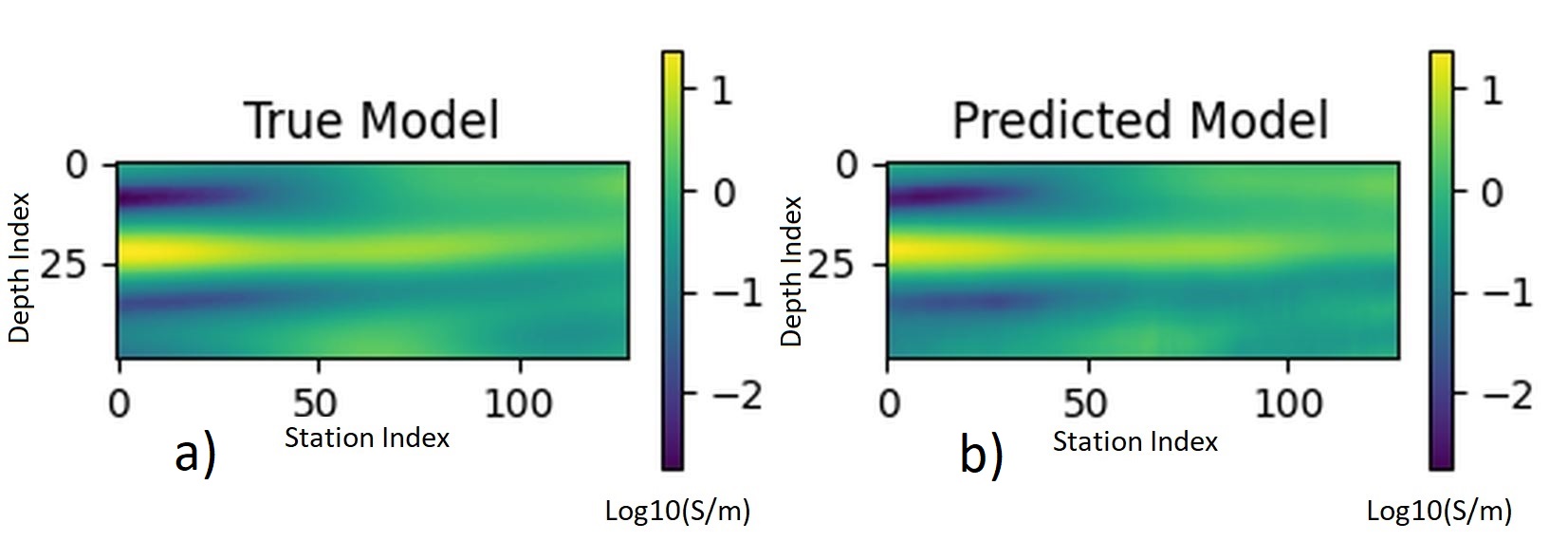
Our training model set consists of $10,000$ conductivity models with a core size of fine cells of 1280m (width) x 245m (deep), with a mesh size of 10m x 10m x 5m, and an example is shown in Figure 2a. Using the Python gstools library [Müller et al., 2022] we generate random models with structures that are plausible for aquifer bearing geology. To obtain appropriate conductivity distributions for the training models, we first invert the field data using a conventional 1D inversion algorithm (EM1DTM) [Farquharson and Oldenburg, 1996]. Then we use the same conductivity statistics from the 1D inversions to create the training models. While the limitations of 1D inversions are well known, our thesis is that the global distribution of conductivity values is sufficiently accurate to use in building the training models.

The training data are then calculated by forward modeling in 3D high and low-moment Skytem data with H3DTD [Haber et al., 2007]. The AEM data, flight heights and labels are all normalized by the standard deviation prior to entering the neural network, while the labels also have the mean subtracted before normalization. The network is first trained and then predictions are made on the high and low-moment field data.

Figure 2: Validation example after training. a) True model. b) Predicted model from validation.

5 Results

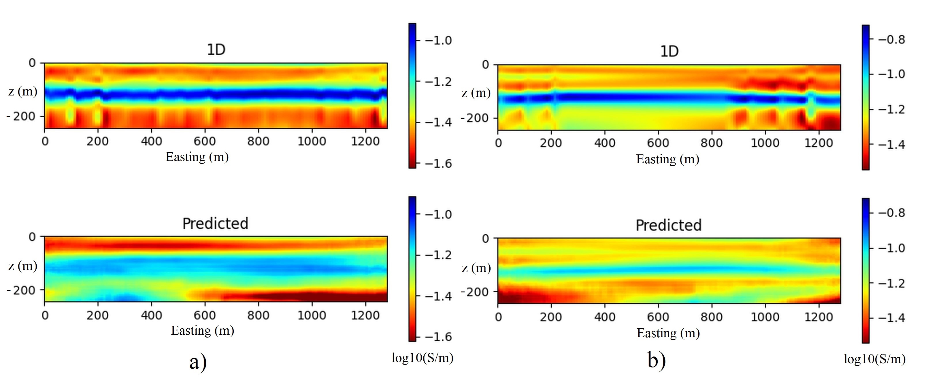
In training, the validation loss flattened out at roughly 800 epochs to a loss of 0.1, and an example of a typical validation result is shown in Figure 2b, where the validation is close to the true image. We then tested the network on the Kaweah field dataset where an example of the normalized input data (high-moment) along with the raw flight heights from a line section is shown in Figure 3. Network predictions, from two line sections along with stitched-1D inversions for reference are displayed in Figure 4.

Figure 3: Field data example from Kaweah. Top) High-moment normalized data. Bottom) Flight heights.

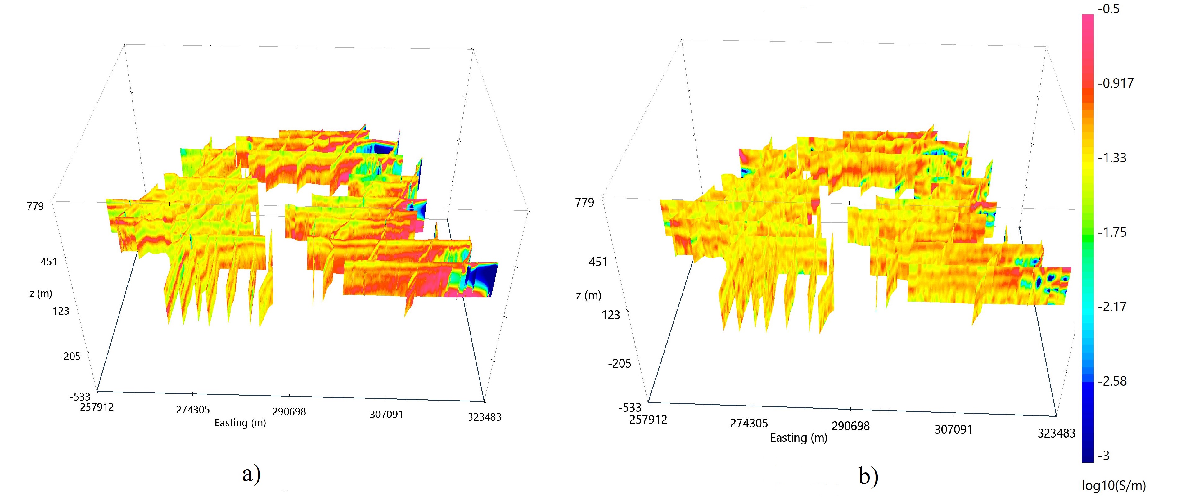
It is clear that the network predictions have many similarities to the 1D inversions, which suggests that the predictions are producing reasonable results. The exact conductivities are slightly different as are the precise geometries of the horizontal layers, but the overall look and feel is similar. For a broader look at all the results, the stitched 1D inversions and network predictions are displayed in Figure 5. The predictions, which take only a matter of seconds to create, produce similar conductivity structures in each line compared to the 1D results, but the stitched 1D inversions produce horizontal layers that are better defined and with more resolution. Therefore, to achieve the same resolution, and eventually even better, compared to the stitched 1D results, we need more training models. $10,000$ is still a tiny number of training models in the machine learning space, and we expect the prediction results to improve as we increase this number, with the added benefit of avoiding 1D pant-leg artifacts with vertical conductors.

Figure 4: Network predictions from two line sections from the Kaweah sub-basin dataset. Results from stitched 1D inversions are shown in the top panel and from the trained network in the bottom panel. Note: z = 0m represents the top of the model and not sea-level.

Figure 5: Skytem Kaweah dataset results a) Stitched 1D inversions. b) Neural network predictions.

6 Conclusions

In this study we trained a neural-network to predict 2D conductivity models from time-domain AEM data, thus bypassing the need for expensive forward modeling during inversion. To train the network, $10,000$ synthetic models were created with similar conductivity attributes to the field data environment and synthetic AEM data were calculated in 3D over these training models. These data were used to train and validate the network, and then we predicted on field data from Kaweah in California and compared the predictions to stitched 1D inversion results. The AI predictions compared well with the 1D results, but did not quite show as much resolution in the horizontal layering. We see this as a successful proof of concept and we are confident that the results will improve with the addition of more training models.

References

- Farquharson and Oldenburg [1996] C. G. Farquharson and D. W. Oldenburg. Approximate sensitivities for the electromagnetic inverse problem. Geophysical Journal International, 126:235–252, 7 1996. ISSN 0956540X. doi: 10.1111/j.1365-246X.1996.tb05282.x. URL http://gji.oxfordjournals.org/cgi/doi/10.1111/j.1365-246X.1996.tb05282.x.
- Wilson et al. [2006] G. A. Wilson, A. P. Raiche, and F. Sugeng. 2.5d inversion of airborne electromagnetic data. Exploration Geophysics, 37:363–371, 2006. ISSN 18347533. doi: 10.1071/EG06363.
- Haber et al. [2007] Eldad Haber, Douglas W. Oldenburg, and R. Shekhtman. Inversion of time domain three-dimensional electromagnetic data. Geophysical Journal International, 171:550–564, 11 2007. ISSN 0956540X. doi: 10.1111/j.1365-246X.2007.03365.x. URL http://doi.wiley.com/10.1111/j.1365-246X.2007.03365.x.
- McMillan et al. [2015] Michael S. McMillan, Christoph Schwarzbach, Eldad Haber, and Douglas W. Oldenburg. 3d parametric hybrid inversion of time-domain airborne electromagnetic data. Geophysics, 80:K25–K36, 9 2015. ISSN 0016-8033. doi: 10.1190/geo2015-0141.1. URL http://library.seg.org/doi/10.1190/geo2015-0141.1.
- Wu et al. [2022] Sihong Wu, Qinghua Huang, and Li Zhao. Instantaneous inversion of airborne electromagnetic data based on deep learning. Geophysical Research Letters, 49, 5 2022. ISSN 19448007. doi: 10.1029/2021GL097165.
- Ronneberger et al. [2015] Olaf Ronneberger, Philipp Fischer, and Thomas Brox. U-net: Convolutional networks for biomedical image segmentation. International Conference on Medical Image Computing and Computer-Assisted Intervention, pages 234–241, 5 2015. URL http://arxiv.org/abs/1505.04597.
- He et al. [2016] Kaiming He, Xiangyu Zhang, Shaoqing Ren, and Jian Sun. Deep residual learning for image recognition. Proceedings of the IEEE conference on computer vision and pattern recognition, pages 770–778, 2016. URL http://image-net.org/challenges/LSVRC/2015/.
- McMillan et al. [2021] Michael S. McMillan, Eldad Haber, Bas Peters, and Jennifer Fohring. Mineral prospectivity mapping using a vnet convolutional neural network. Leading Edge, 40:99–105, 2 2021. ISSN 19383789. doi: 10.1190/tle40020099.1.
- Kingma and Ba [2014] Diederik P. Kingma and Jimmy Ba. Adam: A method for stochastic optimization. arXiv preprint arXiv:1412.6980, 12 2014. URL http://arxiv.org/abs/1412.6980.
- Sørensen and Auken [2004] Kurt I Sørensen and Esben Auken. Skytem – a new high-resolution transient electromagnetic system. Exploration Geophysics, 35:191–199, 2004. ISSN 0812-3985. doi: 10.1071/EG04194.
- Kang et al. [2022] Seogi Kang, Rosemary Knight, and Meredith Goebel. Improved imaging of the large-scale structure of a groundwater system with airborne electromagnetic data. Water Resources Research, 58, 4 2022. ISSN 19447973. doi: 10.1029/2021WR031439.
- Müller et al. [2022] Sebastian Müller, Lennart Schüler, Alraune Zech, and Falk Heße. Gstools v1.3: a toolbox for geostatistical modelling in python. Geoscientific Model Development, 15:3161–3182, 2022.