Effects of resonant dipole-dipole interactions in the spin noise of atomic vapors

Abstract

We perform spin noise spectroscopy close to resonance in a 1-mm-thick cell containing a dense Rubidium vapor. A laser is used to excite optical dipoles in the vapor while probing the Faraday rotation noise. We report unusual lineshapes of the spin noise spectra with a strong density dependence, which we attribute to interactions arising between particles in the system. Introducing a two-body model and simulations, we show that these features are the hallmark of a strong dipole-dipole interaction between binaries within the ensemble. A precise fit of the experimental spectra allows to extract the strength and the duration of the dipole-dipole interaction. We unveil its impact on the spin noise frequency and investigate the role of the atomic motion in the unexpected lineshapes. This work demonstrates the potential of spin noise spectroscopy to observe and quantify strong interactions occurring within a particle ensemble.

I Introduction

The optical measurement of spontaneous angular momentum fluctuations in particle ensembles, called spin noise spectroscopy (SNS), has gained interest over the last decades Aleksandrov and Zapasskii (1981); Crooker et al. (2004). It was shown first to be an efficient, non-invasive way to characterize spin dynamics in dilute atomic vapors, including for example alkali vapors Katsoprinakis et al. (2007); Mihaila et al. (2006); Fomin et al. (2020) or metastable helium vapors Liu et al. (2022, 2023). The method was then extended to study spin noise in condensed phases such as semiconductors Hübner et al. (2014), quantum wells Poltavtsev et al. (2014) or quantum dots Crooker et al. (2010); Glasenapp et al. (2016); Gundín et al. (2024), giving new insights on the relaxation and decoherence channels appearing in strongly-correlated matter. In atomic ensembles, SNS reveals ground-state energy structures both in non-invasive Crooker et al. (2004); Zapasskii et al. (2013); Swar et al. (2021) and invasive Glasenapp et al. (2014); Chalupczak and Godun (2011); Horn et al. (2011); Swar et al. (2018) regimes. The latter has gained considerable interest in the last decade, since it allows to characterize the effects of various forces applied on the system by its environment. Indeed, coupling a system with external fields may drive it out of equilibrium, allowing to obtain information beyond the fluctuation-dissipation theory Sinitsyn and Pershin (2016); Li et al. (2013). For instance, the coupling induced by a radiofrequency field between Zeeman sublevels was characterized using SNS Glasenapp et al. (2014), and randomly fluctuating magnetic fields were shown to give rise to non-thermal spin noise in weakly-pumped atomic ensemble Delpy et al. (2023a). Such field can be responsible for non-Gaussian spin dynamics, as revealed recently by higher-order spin noise (SN) spectroscopy Li et al. (2016).

However, the literature about the use of SNS to probe interactions within an ensemble is much less prolific. So far, only short range interactions have been found to have a strong impact on the spin dynamics in atomic ensembles. Namely, the effect of spin-exchange (SE) collisions has been extensively studied during the past years. SE mechanism has been long understood to be a source of spin fluctuations as well as a source of decoherence and relaxations, according to the fluctuation-dissipation relation Katsoprinakis et al. (2007), and was shown to create spontaneous coherences between hyperfine levels in one-species Mouloudakis et al. (2022) and two-species systems Mouloudakis et al. (2019); Dellis et al. (2014); Roy et al. (2015). However, the spin noise spectra arising from such impact-like interactions are essentially that of independent particles Mouloudakis and Kominis (2021). The SE mechanisms being too short-ranged, experiments never reported any many-body effects mediated by such an interaction. On the other hand, long-range interactions such as resonant dipole-dipole coupling are well known for changing the optical properties of a dense set of emitters, giving rise to coherent processes such as superradiance Gross and Haroche (1982), collective Lamb shifts Röhlsberger et al. (2010); Keaveney et al. (2012); Peyrot et al. (2019), or self-broadening of the optical response of the vapor Lewis (1980). These interactions can create bipartite entanglement, for instance between Rydberg atoms Browaeys et al. (2016), and are the key ingredients for a class of atomic quantum simulators Browaeys and Lahaye (2020).

Therefore, this article studies high-density SNS regimes, in which long-range dipole-dipole coupling are expected to modify the properties of the vapor. We investigate the changes that such interactions can induce on the dynamics of the ground-state populations and coherences of the atoms. We analyze both experimental and numerical spin noise spectra to show the modifications of the usual spectral features due to the presence of the dipole-dipole interaction (DDI) in a dense Rubidium vapor. This article aims at giving a deeper, quantitative insight on the action of the dipole-dipole coupling on spin noise spectra, eventually supporting the results presented in the letter Delpy et al. (2024).

This paper is organized as follows. Section II describes the experimental apparatus and reports experimental SN spectra that exhibit unexpected, density-dependent changes at high densities. Section III then proposes a microscopic toy-model to simulate the spin noise spectra of a system of two atoms coupled by resonant dipole-dipole interactions. We further support these simulations by calculating perturbatively the action of the coupling Hamiltonian on the two-body ground-state energies. Finally, section IV includes the atomic motion and demonstrates its influence on the experimental results in terms of inhomogeneous broadening of the spin noise lines. Eventually, it highlights the link between the low-frequency noise and the finite correlation time of the bipartite system. We indeed show that this specific feature is another proof of the correlations induced in the ensemble by the dipole-dipole interaction.

II Experimental observations

We describe the experimental setup and highlight the specificities and purpose of the vapor cell we use. We then compare the spin noise spectra obtained at low and high atomic densities.

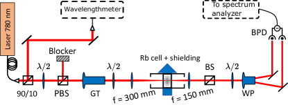
Figure 1: Schematics of the typical setup used to perform SNS experiments shown in the paper. PBS : polarizing beam splitter, GT : Glan-Thomson polarizer, BS : beam splitter, WP : Wollaston prism. BPD : balanced photodetector.

II.1 Experimental setup and results

A schematics of the apparatus is shown in figure 1. An external cavity diode laser is tuned at 780 nm with a power of a few mW to probe spin noise in the vicinity of the $\mathrm{D}_{2}$ line of Rubidium. We use a Glan-Thomson polarizer to ensure a better linear polarization of the beam. It is then focused into the vapor cell to reach a diameter of about $\phi\simeq 300$ µm. The vapor cell is embedded in a metallic oven, the temperature of which is fine-tuned using a homemade temperature controller. The typical achievable temperatures range from ambient temperature to around 180^∘C. After propagating through the cell, the laser beam is sent on a balanced detection. Indeed, we probe the spin noise in the vapor by measuring the stochastic Faraday-like rotations of the probe polarization $\delta\theta(t)\propto\langle S_{z}\rangle(t)$ where $S_{z}$ is the projection of the collective spin on the laser propagation axis $z$ Aleksandrov and Zapasskii (1981); Crooker et al. (2004); Mihaila et al. (2006). A half-wave (HW) plate followed by a Wollaston prism (WP) splits the beam in two well-balanced parts of orthogonal polarization, which are then sent on two photodiodes. The difference of the photocurrents is then proportional to the tiny Faraday rotation angle: $\Delta I=I_{+}-I_{-}\propto\delta\theta(t)$. We feed this differential photocurrent in an electrical spectrum analyzer (ESA) to get the SN spectrum of the atomic vapor, e.g the power spectral density PSD($S_{z}$). Following usual SNS setups Aleksandrov and Zapasskii (1981); Crooker et al. (2004), a pair of coils is used to create a transverse magnetic field aligned along the $x$ axis, essentially forcing the spontaneous spin coherences to oscillate at the Larmor frequency, typically a few MHz. Consequently, the spin noise resonances appear in a region of the spectrum which is free of low-frequency technical noises other than the laser shot noise and the ESA electronic noise background.

The atomic sample is a 1-mm glass cell, containing both ⁸⁵Rb and ⁸⁷Rb isotopes with natural abundance. We do not use any buffer gas, meaning that the vapor is mainly inhomogeneously broadened by Doppler effect. The main asset of using such a small cell is that we can probe SNS at densities as high as $N_{at}=4\times 10^{14}\,\mathrm{at.cm}^{-3}$ while keeping our probe weakly detuned from the center of the ground state hyperfine levels absorption lines. We define the laser detuning as $\Delta=\omega_{p}-\omega_{0}$ with $\omega_{p}$ the laser frequency and $\omega_{0}$ the $F=3\rightarrow F^{\prime}$ hyperfine transition frequency between the $5^{2}S_{1/2}$ and $5^{2}P_{3/2}$ states of ⁸⁵Rb.

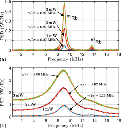
Figure 2: (a) Spin noise spectra obtained for a detuning of $\Delta/2\pi=1.5\,\mathrm{GHz}$, a magnetic field of around 19 G and a vapor density of $N_{at}\simeq 2.5\times 10^{12}\,\mathrm{at.cm}^{-3}$. (b) Spectra obtained in the same conditions except for a higher density of $N_{at}\simeq 3\times 10^{14}\,\mathrm{at.cm}^{-3}$. They all show unexpected linewidths of more than 1 MHz. All dashed lines are fits to the data, using the procedure described in section II.B.

The experimental results shown in this article are obtained for a $\Delta/2\pi=1.5\,\mathrm{GHz}$ detuning. This corresponds to a probe laser tuned halfway between the $F=3\rightarrow F^{\prime}$ and $F=2\rightarrow F^{\prime}$ hyperfine transition of ⁸⁵Rb, so that the spin noise probed here is that of all ground-state hyperfine levels of ⁸⁵Rb and ⁸⁷Rb. Figure 2 (a) shows typical SN spectra for a cell temperature T$=90^{\circ}$C, corresponding to an atomic density $N_{at}\simeq 2.5\times 10^{12}\,\mathrm{at.cm}^{-3}$ using Killian’s formula Weller et al. (2011). The signal background, mainly arising from the laser shot noise, has been independently measured and subtracted. In this condition, the SN spectra exhibit two spin noise resonances because of the different Landé factors of the two Rubidium isotopes. Both peaks are well separated and their widths are about $\gamma/2\pi\simeq 270\,\mathrm{kHz}$, corresponding mainly to the decoherence rate due to the finite time of interaction between the moving atoms and the laser beam. It can be seen in figure 2 (a) that increasing the probe laser power enhances the signal to noise ratio Mihaila et al. (2006); Glazov and Zapasskii (2015), but essentially leaves the linewidth unchanged. This means that the excitation of the ground-state population by the probe beam can be neglected for this detuning. These spectra are totally consistent with the ones reported typically for non-invasive SNS in alkali vapors Crooker et al. (2004); Katsoprinakis et al. (2007); Swar et al. (2018).

Strikingly, figure 2(b) demonstrates that such behaviour is no longer valid at high densities. It shows SN spectra obtained in the same conditions, but at a higher temperature $T=175^{\circ}$C, which corresponds to an atomic density $N_{at}\simeq 3\times 10^{14}\,\mathrm{at.cm}^{-3}$. In such conditions, spin noise resonance lines are much broader, reaching linewidths of more than 1 MHz. Moreover, figure 2(b) shows that increasing the probe laser power from 1 mW to 3 mW results in a increase of the linewidths, eventhough the power broadening has been ruled out by the results at low density. Finally, a large asymmetry in the lineshape appears, caused by an additional low-frequency noise on top of the subtracted noise floor.

II.2 Density-dependent anomalous broadening

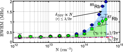
Figure 3: Evolution of the spin noise linewidths as a function of the vapor atomic density for both isotopes. The dashed line and dash-dotted line correspond to the expected transit rate and the sum of transit and SE collisional rates for single-atom dynamics, respectively. The laser power is 2 mW and the detuning is $\Delta/2\pi=1.5\,\mathrm{GHz}$.

Let us first study the spin noise linewidths of both isotope peaks as a function of the atomic density. We fit the lineshapes using a sum of three functions. The first one is a broad Lorentzian line centered on zero frequency, which accounts for the extra low-frequency noise. The two other lines correspond to the spin resonance peaks of both ⁸⁵Rb and ⁸⁷Rb isotopes, and are given by:

$$C_{zz}(\omega)=A\times\dfrac{\gamma^{2}+\omega^{2}+\omega_{L}^{2}}{(\gamma^{2}+\omega_{L}^{2}-\omega^{2})^{2}+4\gamma^{2}\omega^{2}}$$ (1)

These specific lineshapes arise from the Bloch equations describing the spin precession around a magnetic field aligned with the $x$ axis, under the action of a damping and a white-noise forcing term. The Bloch equations can be written under the matrix form

$$\bm{\dot{S}}=R\bm{S}+G\bm{\eta}$$ (2)

with $\bm{S}=\begin{pmatrix}S_{y}\\ S_{z}\end{pmatrix}$, $R=\begin{pmatrix}-\gamma_{L}&\omega_{L}\\ -\omega&-\gamma_{L}\end{pmatrix}$ the deterministic drift matrix, and $\bm{\eta}=\begin{pmatrix}\eta_{y}\\ \eta_{z}\end{pmatrix}$ a stochastic variable with a zero mean and unit variance, accounting for the spin fluctuations. The matrix $G$ describes the strength of the spin noise, and we simply take $G\equiv\sqrt{A}\times 1\kern-2.5pt\text{l}$, $A$ being a free parameter in the fit. The variable $\bm{S}$ obeying such an equation is a vectorial Ornstein-Uhlenbeck process, which admits a power spectrum matrix Katsoprinakis et al. (2007); Sinitsyn and Pershin (2016); Mouloudakis et al. (2022) given by:

$$C(\omega)=(R+i\omega 1\kern-2.5pt\text{l})^{-1}GG^{T}(R^{T}-i\omega 1\kern-2.5pt\text{l})^{-1}.$$ (3)

The power spectral density (PSD) of $S_{z}$ is given by the element $C_{zz}(\omega)$, which yields the result of eq.(1).

Figure 3(a) shows the changes in the spin noise half-width at half maximum (HWHM), for densities ranging from $10^{12}\,\mathrm{at.cm}^{-3}$ to $4\times 10^{14}\,\mathrm{at.cm}^{-3}$. A drastic increase of the linewidths of both spin noise peaks is visible, reaching almost $2\,\mathrm{MHz}$ for ⁸⁵Rb at T$=180^{\circ}$C. Strikingly, this density-dependent broadening cannot be explained by the usual relaxation mechanisms, namely transit decoherence and spin-exchange collisions. The expected linewidths corresponding to these processes are shown as baselines in dashed line (transit rate $\gamma_{t}/2\pi$) and dash-dotted line (sum of transit and SE collisional rate $\gamma_{t}/2\pi+\gamma_{se}/2\pi$) in figure 3. The shaded area thus represent an additional broadening that remains unexplained by the single-spin dynamics. Interestingly, the onset of this density-dependent broadening appears as soon as the density of the vapor reaches $10^{14}\,\mathrm{at.cm}^{-3}$, corresponding to an average inter-atomic distance of around $\langle r\rangle\simeq 0.55N_{at}^{-1/3}\simeq 120\,\mathrm{nm}$ Chandrasekhar (1943), which we denote $r_{0}$ in the rest of the paper. This typical distance being close to the reduced wavelength $\lambda/2\pi$ of the nearest transition, this onset suggests the appearance of radiative coupling between atoms in the vapor, which we discuss in section III.

II.3 Analysis of the additional low-frequency noise

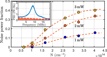
Figure 4: Fraction of the noise power contained in the low-frequency component as a function of the vapor density, measured for probe power of $1\,\mathrm{mW}$, $2\,\mathrm{mW}$ and $3\,\mathrm{mW}$. The orange dashed line are guides to the eye. Inset: the shaded area shows the region of the spectra integrated to get the low-frequency noise power.

Let us now describe the low-frequency tail appearing for atomic densities higher than $N_{at}=10^{14}\,\mathrm{at.cm}^{-3}$. This noise cannot be attributed to shot noise as we measured it independently and subtracted it from the data. This extra component is highlighted in color in the inset of figure 4, which shows a spectrum obtained for a temperature of $T=175^{\circ}$C ($N_{at}=3\times 10^{14}\,\mathrm{at.cm}^{-3}$) and a probe power of $2\,\mathrm{mW}$. As explained in the previous subsection, we fit this broad line using a Lorentzian function centered on the zero frequency, with amplitude and width being free parameters. The HWHM is estimated to be $\gamma_{c}/2\pi=14.1\pm 0.8\,\mathrm{MHz}$. To be more quantitative, we compare the ratio of the noise power contained in this area over the total noise power as a function of the density of the vapor. Figure 4 shows that this fraction increases with the vapor density. It is not measurable with precision below $N=10^{14}\,\mathrm{at.cm}^{-3}$, but increases afterwards up to non-negligible values. For $3\,\mathrm{mW}$ of light power and a density of $N=4\times 10^{14}\,\mathrm{at.cm}^{-3}$ (180^∘C), almost half of the total power is contained in the low-frequency component. Furthermore, the laser power has a large impact on the variance of this noise: the fraction of the total spin noise contained in the low frequency component is three times larger at the highest density for a $3\,\mathrm{mW}$ probe power than for $1\,\mathrm{mW}$. This demonstrates that the probe laser plays a crucial role in the creation of this noise, in accordance with our earlier suggestion of an optical coupling appearing within the system.

III Microscopic model: numerical simulations and perturbative treatment of the DDI

In the previous section, we quantified the density dependence of the spin noise lineshapes measured at high atomic densities. Such experimental observations suggest the appearance of a strong optical coupling regime. In this section, we propose a simple microscopic model of two atoms coupled via resonant dipole-dipole coupling and then numerically study the spin noise spectra obtained in the case where the atoms are static. We highlight drastic changes in the spectra, which we subsequently explain using perturbative calculations of the two-body ground-state energy structure.

III.1 Model

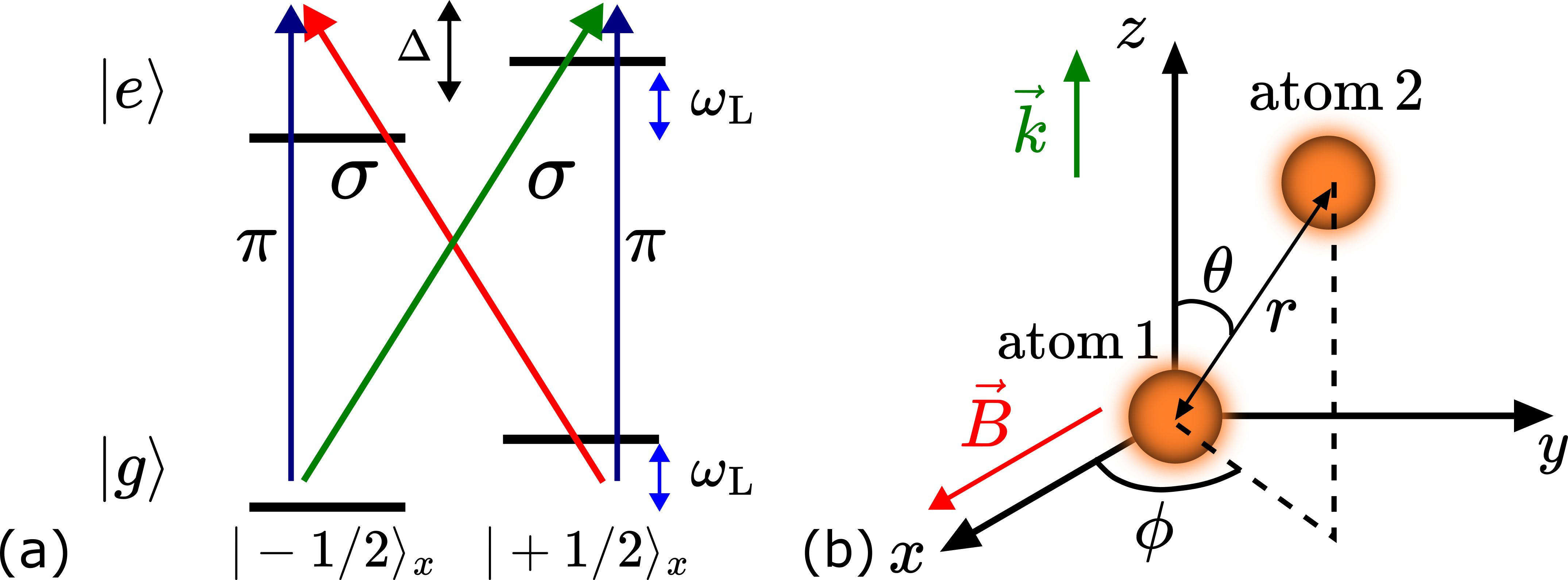
Figure 5: (a) Single-particle energy diagram considered in our model, quantized in the $x$ direction, along the magnetic field. $\pi$ ($\sigma$) denotes light polarized along the $x$ ($y$) axis. The light is detuned by $\Delta$ from the center of the resonance. (b) Schematics and parameters used to describe the spatial arrangement of the two-body problem: one atom is at the origin of the frame and the spherical coordinates give the position of the second atom.

Lets us now introduce the model derived to explain the experimental SN spectra. Since we can neglect the SE collisions rate compared to the transit rate, we make the assumption that inter-hyperfine coherences do not play a role. We can thus overlook the hyperfine structures of the atoms and consider only one ground-state and one excited state. Moreover, we do not aim at describing higher-order tensorial arrangements of spins Fomin et al. (2020); Liu et al. (2023) but only spin orientation. Consequently, it is reasonable to consider only a $J=1/2$ ground state to simulate the dynamics of spin coherences. The magnetic field is aligned along the $x$ axis, thus splitting the ground-state Zeeman sublevels by an energy $\hbar\omega_{L}$. Figure 5 (a) shows a schematics of this configuration, with a quantization axis in the direction of the magnetic field. Since we want to investigate the action of the probe beam on the optical coupling, we also include a $J^{\prime}=1/2$ excited state. The light then couples the ground-state Zeeman manifold to the excited one. As the light propagates along the $z$ axis, a linear polarization along the $x$ axis ($\pi$-polarized) couples ground- and excited-states Zeeman sublevels with the same spin projection $m_{S}$ along the $x$ axis. Orthogonally polarized light ($\sigma$ polarization) couples Zeeman sublevels of opposite values of $m_{S}$. It is important to notice that for the sake of the discussion performed in this section, this choice of quantization axis is not the same as in the letter Delpy et al. (2024). With this choice, we recall that the spin noise $\braket{S_{z}(t)}$ arises from fluctuating coherences between the ground-state Zeeman sublevels $\ket{g,-1/2}_{x}$ and $\ket{g,+1/2}_{x}$, where $g$ denotes the ground-state.

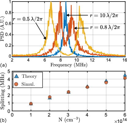
Figure 6: (a) Examples of three spin noise spectra obtained for a fixed geometry with three average interatomic distance $r$ and fixed angles $\theta=0,\,\phi=0$. (b) Orange dots: Numerical calculations of the splitting between the peaks as a function of the density $N=(0.55/r)^{3}$. Blue triangles: theoretical expression using the calculations of section III.C.

Let us now include the dipole-dipole interaction. We consider two atoms with the single-atom energy structure described above. The uncoupled part of the Hamiltonian is thus

$$H_{0}=\sum_{i=1,2}H_{SA}^{(i)},$$ (4)

with $H_{SA}^{(i)}=\hbar\omega_{L}S_{x}^{(i)}-\mathbf{D}^{(i)}\cdot\mathbf{E}(\bm{r}_{i},t)$, where $\bm{r}_{i}$ denotes the position of the atom $i$, is the single-atom hamiltonian including Zeeman splitting and light-matter coupling. Here, we choose to work in the long wavelength approximation, i.e. we assume that the atoms are close enough to neglect the dependence on $\bm{r}_{i}$ of the electric field $\mathbf{E}(\bm{r}_{i},t)=\mathbf{E}(t)$. We thus neglect the phase difference in the oscillations of the atomic dipoles. This approximation is justified by our experimental observations: the impact of the DDI on the SN spectra is shown to be relevant only when the interatomic distance is smaller than $\lambda/2\pi$, i.e. when the approximation becomes valid. For large interatomic separation, this approximation breaks down. Nevertheless, as discussed later in the paper, the radiative coupling has no impact in this case.

This coupling between the two atoms can now be included by considering the interaction of both atoms with the vacuum modes of the electromagnetic field bath Lehmberg (1970); Agarwal (2012); Le Kien and Rauschenbeutel (2017); Reitz et al. (2022). Following the standard derivation of the master equation, we trace out the bath degree of freedom to get the following equation of motion:

$$\dot{\rho}=-\dfrac{i}{\hbar}\left[H_{0}+V_{dd},\rho\right]+D[\rho]+f,$$ (5)

where the resonant dipole-dipole interaction Hamiltonian is

$$V_{dd}=\hbar\sum_{\begin{subarray}{c}i\neq j\\ \lambda,\lambda^{\prime}\end{subarray}}\zeta_{\lambda,\lambda^{\prime}}(r_{ij})\frac{D_{+}^{\lambda,i}D_{-}^{\lambda^{\prime},j}}{d_{0}^{2}}.$$ (6)

Here, $D_{+}^{\lambda,i}$ (resp. $D_{-}^{\lambda,i}$) is the excitation (resp. de-excitation) part of the dipole operator of atom $i$ and of polarization component $\lambda=\sigma_{+},\sigma_{-},z$. We denote $d_{0}$ the dipole element for the $J\rightarrow J^{\prime}$ transition and $\Gamma_{0}$ the excited states population relaxation rate. The quantity $\displaystyle{\zeta_{\lambda,\lambda^{\prime}}(r_{ij})=-\dfrac{3\Gamma_{0}}{4}\,\left(\bm{\varepsilon}_{\lambda}\right)^{*}\cdot\mathrm{Re}\quantity(\overline{\overline{G}}(\mathbf{r}_{i},\mathbf{r}_{j},\omega_{0}))\cdot\bm{\varepsilon}_{\lambda^{\prime}}}$, where $\displaystyle{\overline{\overline{G}}(\mathbf{r}_{i},\mathbf{r}_{j},\omega_{0})=\quantity(\overline{\overline{1\kern-2.5pt\text{l}}}+\dfrac{\bm{\nabla}\bm{\nabla}}{k^{2}})\dfrac{e^{ik_{0}r_{ij}}}{k_{0}r_{ij}}}$ is the electromagnetic Green’s dyadic, gives the strength of the radiative coupling between a dipole in $\mathbf{r}_{i}$ polarized along $\bm{\varepsilon}_{\lambda^{\prime}}$ and a second one placed in $\mathbf{r}_{j}$ oscillating in the direction of $\bm{\varepsilon}_{\lambda}$. Here we denoted $k_{0}=\omega_{0}/c$ the light wave vector and $r_{ij}=|\mathbf{r}_{i}-\mathbf{r}_{j}|$ the interatomic distance. The symmetrical tensor $\overline{\overline{\zeta}}(r_{ij})$ thus strongly depends on the interatomic geometry, and particularly on the distance between two atoms :

$$\centering\begin{array}[]{c c l}\overline{\overline{\zeta}}(r_{ij})&=&\dfrac{3\Gamma_{0}}{4}\left(\dfrac{\cos\xi}{\xi^{3}}+\dfrac{\sin\xi}{\xi^{2}}-\dfrac{\cos\xi}{\xi}\right)1\kern-2.5pt\text{l}\\ &&+\dfrac{3\Gamma_{0}}{4}\left(\dfrac{\cos\xi}{\xi}-\dfrac{3\cos\xi}{\xi^{3}}-\dfrac{3\sin\xi}{\xi^{2}}\right)\mathbf{n}\otimes\mathbf{n},\\ \end{array}\@add@centering$$ (7)

where $\xi=k_{0}r_{ij}$ and $\mathbf{n}=\mathbf{r}_{ij}/r_{ij}$ is the unit vector in the interatomic direction. The decoherence matrix $D[\rho]$ takes the form

$$\begin{split}D[\rho]=&-\gamma_{t}\rho-\sum_{\begin{subarray}{c}i,j\\ \lambda,\lambda^{\prime}\end{subarray}}\dfrac{\gamma_{\lambda,\lambda^{\prime}}(r_{ij})}{d_{0}^{2}}[D_{+}^{\lambda,i}D_{-}^{\lambda^{\prime},j}\rho\\ &-\rho D_{+}^{\lambda,i}D_{-}^{\lambda^{\prime},j}-2D_{-}^{\lambda^{\prime},j}\rho D_{+}^{\lambda,i}],\end{split}$$ (8)

where

$$\gamma_{\lambda,\lambda^{\prime}}(r_{ij})=\dfrac{3\Gamma_{0}}{4}\,\left(\bm{\varepsilon}_{\lambda}\right)^{*}\cdot\mathrm{Im}\quantity(\overline{\overline{G}}(\vec{r}_{i},\vec{r}_{j},\omega_{0}))\cdot\bm{\varepsilon}_{\lambda^{\prime}}$$ (9)

is the decoherence rate due to the coupling with the electromagnetic field modes. The first term in the definition of $D[\rho]$ accounts for the averaged transit relaxations. We include the spin fluctuations by using a noise operator $f$ similar to the one introduced in refs. Liu et al. (2022, 2023); Delpy et al. (2023a). This Hermitian, traceless operator introduces white-noise fluctuations in the Zeeman population and coherences. This way, we mimic the Poissonian transit of the atoms through the beam, which is the main mechanism of noise in our case. The equation of motion given by eq.(5) is used to simulate the time evolution of the two-atom density matrix. To correctly take into account the action of the light on the atomic population and coherences, we start from an uncorrelated thermal state $\rho_{0}=\rho_{th}^{(1)}\otimes\rho_{th}^{(2)}$ and let it evolve towards a steady-state density matrix under the action of the magnetic field and the light beam. After it is reached, we add the fluctuations operator in eq.(5) and start simulating a set of noisy time traces. For each of them, we compute the quantum average of the two-atom spin operator $\braket{S_{z}}=\sum_{i=1,2}\mathrm{Tr}(\rho s_{z}^{(i)})$, with $s_{z}^{(i)}$ the single-particle spin operator. From this set of data we can then compute the PSD of $\braket{S_{z}}$ and thus obtain the two-body SN spectra. It should be here mentioned that we do not average over the Doppler effect experienced by the atoms, and comparison with experimental results should thus be done with parameters that keep the ratio $\Delta/\Gamma$ constant, where $\Gamma$ is the optical coherence decay rate of one atom: this allows to have the same absorption for the experiments and simulations. While it is usual to increase $\Gamma$ to the Doppler width value and keep the optical detuning equal to the experimental value, we chose to have $\Gamma$ equal to the atom homogeneous linewidth $\Gamma_{0}/2$, and decrease $\Delta/2\pi$ down to 300 MHz, which helps us to save computing time.

III.2 Simulation of spin noise spectra: results in static geometry

We first consider the ideal case where the atoms are fixed in the lab frame. The geometry and the definition of the coordinates are shown in figure 5(b). We chose arbitrary spherical angles $\theta$ and $\phi$ between the atoms, as well as a fixed interatomic distance $r$. In that case, the two-body problem is characterized by the interatomic vector $\mathbf{r}_{ij}$. This in turn fully determines the Green’s tensor $\overline{\overline{G}}(\mathbf{r}_{i},\mathbf{r}_{j},\omega_{0})$ as well as the interaction Hamiltonian and decoherence operators Lehmberg (1970); Agarwal (2012). The main result of such a configuration is the following: for large interatomic distances $r>\lambda/2\pi$, the SN spectrum obtained is essentially that of a single spin, while it can dramatically change when $r\leq\lambda/2\pi$. For instance, fig.6(a) shows spectra obtained for $\theta=0$ and $\phi=0$, and three interatomic distances. For $r>\lambda/2\pi$, we obtain a single and typical SN resonance. However, for $r\leq\lambda/2\pi$, two lines are clearly visible. This remarkable splitting is plotted as a function of the vapor density from which we infer the average interatomic distance $r$ in figure 6(b) (orange dots). As the atomic density increases, it gets larger, eventually reaching several MHz at the highest density. Assuming that the splitting is due to DDI Hamiltonian, such an increase with the density can be understood considering the fact that $\zeta_{\lambda,\lambda^{\prime}}(r_{ij})$ is an increasing function of $1/r$ (see eq.(7)), eventually scaling like $1/r^{3}\propto N$ in the near field Browaeys et al. (2016); Agarwal (2012). The fact that the splitting represented in fig.6(b) is not a perfectly linear function of $N$ can be explained by the fact that $r$ is just smaller than $\lambda/2\pi$ but not much smaller in the range of values studied here. We are thus not strictly speaking in the near-field regime. Moreover, there is no effects on the linewidth of the peaks, since the part of the decoherence operator $D[\rho]$ coming from the radiative coupling does not affect the ground-state coherences, but only the optical dipoles.

However, the interatomic distance $r_{ij}$ is not the only meaningful parameter. Indeed, the angular coordinates $(\theta,\phi)$ rule the intensity of the coupling between the dipoles via the tensor $\mathbf{n}\otimes\mathbf{n}$ appearing in the electromagnetic Green’s dyadic. Therefore, the splitting strongly depends on these angles: appendix A show some $(\theta,\phi)$ couples for which the it is reduced or even vanishes. In the following discussion, we stick to the case ($\theta=0,\,\phi=0$) and analyze the splitting in terms of the perturbation induced by the DDI on the two-atom eigenenergies.

III.3 Physical interpretation

Let us consider the energy diagram shown in figure 5(a). It depicts the single-atom energy structure considered in our model, quantized along the $x$ axis, which is the direction of the transverse magnetic field. Consequently, in the absence of probe light, the single-atom eigenvectors are that of the Zeeman hamiltonian, namely $\ket{g,-1/2}_{x}$ and $\ket{g,+1/2}_{x}$, with respective energies $-\hbar\omega_{L}/2$ and $+\hbar\omega_{L}/2$. This results in the coherences between these two states oscillating at $\omega_{L}$. The spin noise spectra thus show one peak centered at the Larmor frequency. Let us now add a $\sigma$-polarized probe light, which couples the ground-state sublevel $\ket{g,-1/2}_{x}$ to the excited state sublevel $\ket{e,+1/2}_{x}$, and $\ket{g,+1/2}_{x}$ to $\ket{e,-1/2}_{x}$. The new low-energy eigenvectors can be computed analytically. In the experimentally relevant case $\omega_{L}\ll\Delta$, they read

$$\centering\left\{\begin{array}[]{c c l}\ket{-}&=&\cos(\psi/2)\ket{g,-1/2}_{x}+\sin(\psi/2)\ket{e,+1/2}_{x},\\ \ket{+}&=&\cos(\psi/2)\ket{g,+1/2}_{x}+\sin(\psi/2)\ket{e,-1/2}_{x},\\ \end{array}\right.\@add@centering$$ (10)

where the mixing angle $\psi$ is given by $\tan(\psi/2)=\Omega/(2\Delta)$ with $\Omega$ the Rabi frequency of the light. The Clebsch-Gordan (CG) coefficients do not appear in the mixing angle value, as they are here equal for both transitions. In the weak driving limit ($\Omega\ll\Delta$), the mixing angle tends to zero and we can map directly the state $\ket{-}_{x}$ to $\ket{g,-1/2}_{x}$ and $\ket{+}_{x}$ to $\ket{g,+1/2}_{x}$. These new eigenstates of the one-body hamiltonian $H_{SA}^{(i)}$ are the "light-shifted" states with respective eigenenergies $\displaystyle{\mp\frac{\hbar\omega_{L}}{2}+\frac{\Delta-\sqrt{\Delta^{2}+\Omega^{2}}}{2}}$. This shift in frequency is summarized in figure 7 (upper part). Since these states experience similar light shifts, they are still separated by an energy $\hbar\omega_{L}$, and the SN spectrum still show one peak at the Larmor frequency. It is worth noting that experiments already demonstrated large lights shifts visible in spin noise spectra, for instance in metastable helium Delpy et al. (2023b). Although they were also reported in SNS experiments in alkali atoms Chalupczak and Godun (2011), light shifts are less likely to appear in Rubidium in non resonant conditions because of the small hyperfine splitting of the excited states Happer (1970), which makes our model valid.

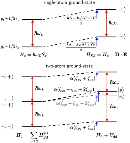
Figure 7: Upper panel: changes in the single-atom ground-state energies due to the light-matter coupling. The perturbed states see their energies impacted by the light shift. Lower panel: changes in the two-atom ground-states induced by the dipole-dipole coupling. The DDI shifts the four state unevenly, resulting in a modification of the spin noise frequencies.

Let us now consider a system of two identical atoms experiencing the influence of both the magnetic field and the light field. We first assume that they are uncoupled, and we move to the two-body Hilbert space. The relevant eigenbasis is thus composed of 16 eigenvectors. Nevertheless, the dynamics of the spin noise emerges from spontaneous coherences arising within the ground-state. The spin noise frequency can therefore be deduced from the structure of the ground-state only, so that we will restrict our analysis to the four lowest energy states. They form the two-body ground-state manifold. Considering the one-atom eigenstates given by eq. (10), we can construct this ground-state manifold: $\{\ket{-,-},\ket{-,+},\ket{+,-},\ket{+,+}\}$. However, since the atoms are uncoupled, the two-body SN spectra are similar to that of a single-atom and thus still show one peak at the Larmor frequency.

We finally add the dipole-dipole interaction in a perturbative manner. We consider the action of the interaction Hamiltonian $V_{dd}$ on the four uncoupled ground-state eigenvectors of the two-body system. With the specific choice of angular coordinates ($\theta=0$, $\phi=0$), one can show that the Green’s tensor $\overline{\overline{G}}(\vec{r}_{i},\vec{r}_{j},\omega_{0})$ is simply diagonal in the basis $\{x,\,y,\,z\}$, i.e. the two atoms are coupled via dipoles with similar polarization in this basis. This yields the following expression for $V_{dd}$:

$$\begin{array}[]{r l}V_{dd}=&\hbar\zeta_{xx}(r_{ij})\left(\dfrac{D_{+}^{x,1}D_{-}^{x,2}}{d_{0}^{2}}+\dfrac{D_{+}^{x,2}D_{-}^{x,1}}{d_{0}^{2}}\right)\\ &+\hbar\zeta_{yy}(r_{ij})\left(\dfrac{D_{+}^{y,1}D_{-}^{y,2}}{d_{0}^{2}}+\dfrac{D_{+}^{y,2}D_{-}^{y,1}}{d_{0}^{2}}\right)\\ &+\hbar\zeta_{zz}(r_{ij})\left(\dfrac{D_{+}^{z,1}D_{-}^{z,2}}{d_{0}^{2}}+\dfrac{D_{+}^{z,2}D_{-}^{z,1}}{d_{0}^{2}}\right).\end{array}$$ (11)

Since we choose a $\sigma$-polarized light, only $\sigma_{+}$ and $\sigma_{-}$ coherences are created, as seen from eq. (10). It is therefore easier to perform calculations using the dipole operator expressed in the $\{x,\sigma_{+},\sigma_{-}\}$ basis according to the transformation:

$$\left\{\begin{array}[]{c c}D^{y}=&\dfrac{D^{\sigma_{+}}+D^{\sigma_{-}}}{\sqrt{2}},\\ D^{z}=&\dfrac{D^{\sigma_{+}}-D^{\sigma_{-}}}{\sqrt{2}i}.\\ \end{array}\right.$$ (12)

Calculating the first-order perturbation induced by the remaining terms on the four uncoupled eigenvectors $\ket{-,-},\ket{+,-},\ket{-,+}$ and $\ket{+,+}$ of the two-body lower manifold is now feasible using eqs.(10), (11) and (12). The relevant terms are given in Appendix B, using diagrams showing the exchange of excitation to which they correspond. Remarkably, the DDI lifts the degeneracy between the states $\ket{+,-}$ and $\ket{-,+}$, to give the new symmetrized states $\displaystyle{\ket{s}=\frac{\ket{+,-}+\ket{-,+}}{\sqrt{2}}}$ and $\displaystyle{\ket{u}=\frac{\ket{+,-}-\ket{-,+}}{\sqrt{2}}}$. One eventually finds that the first-order correction to the set of eigenenergies under the action of the resonant DDI is

$$\left\{\begin{array}[]{c c l}\braket{-,-}{V_{dd}}{-,-}&=&\alpha(\zeta_{yy}+\zeta_{zz}),\\ \braket{+,+}{V_{dd}}{+,+}&=&\alpha(\zeta_{yy}+\zeta_{zz}),\\ \braket{s}{V_{dd}}{s}&=&\alpha(\zeta_{yy}-\zeta_{zz}+2\zeta_{xx}),\\ \braket{u}{V_{dd}}{u}&=&\alpha(\zeta_{yy}-\zeta_{zz}-2\zeta_{xx}),\\ \end{array}\right.$$ (13)

with $\alpha=\dfrac{\Omega^{2}\Delta^{2}/4}{(\Omega^{2}/4+\Delta^{2})^{2}}\simeq\dfrac{\Omega^{2}}{4\Delta^{2}}$ for $\Omega\ll\Delta$. These level shifts due to the DDI are summarized in the bottom panel of figure 7.

The key result of this part is the following: since the four levels do not experience the same shifts, new frequencies appear in the spin noise spectrum. Indeed, the two-atom $z$-axis spin component $\braket{S_{z}}=\sum_{i=1,2}\braket{s_{z}^{(i)}}$ precesses at the frequencies given by

$$\omega\equiv\frac{E_{\ket{a}}-E_{\ket{b}}}{\hbar},$$ (14)

with $\ket{a}$ and $\ket{b}$ two of the two-body ground-states verifying the selection rule $\Delta M_{x}=\pm 1$ Mihaila et al. (2006) where $M_{x}$ denotes an eigenvalue of the two-atom $S_{x}$ operator. Fortunately, the four states $\ket{-,-}$, $\ket{s}$, $\ket{u}$ and $\ket{+,+}$ can be directly mapped to the eigenstates of the two operators $\{S^{2},S_{x}\}$ in the weak driving limit. Indeed, since they originate from the addition of two spin 1/2 systems, the two-atom ground-state levels are either spin 1 or spin 0 states: $\ket{-,-}$, $\ket{+,+}$ and $\ket{s}$ are the spin 1 triplet states, and $\ket{u}$ is the spin 0 singlet state. The frequencies authorized by eq. (14) therefore arise from the difference in energy between the states $\ket{-,-}$ and $\ket{s}$ on the one hand, and between the states $\ket{s}$ and $\ket{+,+}$ on the other hand. The spinless state $\ket{u}$ does not participate in the spin noise spectrum of the system. Consequently, taking into account the energy shifts given by eq.(13), this yields the frequencies

$$\left\{\begin{array}[]{c c}\omega_{+}=&\omega_{L}+\delta\\ \omega_{-}=&\omega_{L}-\delta\end{array}\right.$$ (15)

where $\delta=2\alpha|\zeta_{zz}-\zeta_{xx}|$. These two frequencies are highlighted in the lower panel of fig. 7. This eventually proves how the splitting $2\delta$ visible in figure 6 (a) is a consequence of the changes in the ground-state two-body energies induced by the DDI. The splitting calculated theoretically using the model presented above are presented in blue triangles in fig.6(b), taking into account the CG coefficients that have been let aside here. The excellent agreement validates our physical picture. Only the last points show a slight discrepancy, suggesting the limit of the perturbative approach above $N_{at}=5\times 10^{14}\,\mathrm{at.cm}^{-3}$. We emphasize here a couple of remarkable properties of this analytical result. First, the value of the splitting is proportional to a linear combination of elements of the tensor $\overline{\overline{\zeta}}$. Since these elements all scale with the interatomic distance $r$ like a power law $1/r^{\beta}$, this explains why the splitting of fig.6 (b) follows the same scaling. Furthermore, as expected for the coupling between light-induced dipoles, the splitting scales with the Rabi frequency as $\Omega^{2}$ (i.e. linearly with the laser power) in the weak driving limit. This eventually supports our experimental observations (see fig.2(b) of this paper and fig.4 of the letter Delpy et al. (2024)) that the more intense the light beam, the stronger the interaction.

It has been observed when performing simulations that the polarization of the light matters: when using $\pi$-polarized light, only $\pi$ dipoles are excited among the atoms. One can easily verify that in this case, the diagonal terms of $V_{dd}$ in the uncoupled basis $\{\ket{-,-},\,\ket{-,+}\,\ket{+,-},\,\ket{+,+}\}$ arise solely from the $D_{+}^{x,i}D_{-}^{x,j}$ part of the hamiltonian and are all equal. In spite of the degeneracy of $\ket{+,-}$ and $\ket{-,+}$ still being lifted by other non-diagonal terms, the resulting splitting is greatly reduced as compared to the earlier case of a $\sigma$-polarized light excitation and barely exceeds the linewidth of each peak. However, the experimental spin noise spectra bear no such polarization dependence. This can be understood from the limit of our model, where both ground and excited states are composed of two Zeeman sublevels only, creating a strong sensitivity to light polarization. This sensitivity is reduced in atoms having a larger number of sublevels both in ground and excited states, like for instance alkali atoms such as Rubidium. We would thus expect this dependence to be attenuated in the case of a simulation taking into account e.g. hyperfine levels and sublevels with the corresponding CG coefficients.

Nevertheless, the last section will demonstrate that this simple model remarkably encapsulates the physical ingredients required to explain the experimental observations, as soon as the atomic motion is introduced.

IV Effect of the dipole-dipole interaction in the case of a time-dependent two-atom conformation

While the DDI mechanism highly depends on the spatial arrangement of the atoms, the thermal motion cannot be forgotten. Let us now investigate how it affects the SN spectra in order to recover the experimental observations from our model. We provide details about our numerical procedure, and we conclude on the features obtained in the dynamical regime that were not predicted in the static case.

IV.1 Results of numerical simulations including dynamical two-body conformations

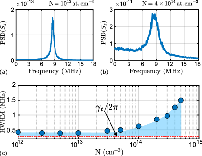
Figure 8: (a,b) Examples of spin noise spectra simulated for densities of $10^{12}\,\mathrm{at.cm}^{-3}$ ($\simeq 75^{\circ}$C) and $4.10^{14}\,\mathrm{at.cm}^{-3}$ ($\simeq 180^{\circ}$C). (c) Simulated evolution of the HWHM of the SN peak as a function of atomic density. Parameters : $\Omega/2\pi=150\,\mathrm{MHz}$, $\Delta/2\pi=300\,\mathrm{MHz}$.

A binary is formed thanks to the DDI when two atoms are nearby in the vapor. As they are moving, the two-body configuration is constantly evolving. We model this effect by including random changes in the atomic spherical coordinates $(r,\theta,\phi)$ after a time of evolution denoted $\tau_{c}$. This time can be therefore be considered as the lifetime of the binary. The interatomic distance $r$ is picked randomly using the nearest-neighbor probability density function and the average atomic density N Chandrasekhar (1943):

$$P(r)=4\pi Nr^{2}e^{-\frac{4}{3}\pi Nr^{3}}.$$ (16)

The two angles $\theta,\phi$ are picked with uniform probability distributions. The spin noise PSD is computed as before using the simulated time-sequence of $\braket{S_{z}}(t)$. Figures 8 (a) and (b) show the results of including a finite lifetime of the binary in such a way. We choose a lifetime of $\tau_{c}=100\,\mathrm{ns}$, much smaller than the duration of the simulations. The result is two-fold. First, the spin noise resonance obtained at a high density $N=4\times 10^{14}\,\mathrm{at.cm}^{-3}$ (spectrum (b)) is much broader than the one at a low-density $N=10^{12}\,\mathrm{at.cm}^{-3}$ (spectrum (a)). Following the discussion led in the previous section, this broadening can now be interpreted as the average over a set of various oscillation frequencies. Indeed, since the interatomic distance and angles fluctuate with time, the two precession frequencies resulting from the action of the DDI are also quickly changing (see fig. 6 for instance). They are thus averaged to yield a broad, continuous spectrum. Furthermore, fig.8 (c) shows the changes in the linewidth of the spectrum as a function of the vapor density. It increases from around $300\,\mathrm{kHz}$ at low densities up to $1.5\,\mathrm{MHz}$ at $N=5\times 10^{14}\,\mathrm{at.cm}^{-3}$. These values are very close to the one observed experimentally and shown in fig.3 (a). Moreover, the difference between the simulated linewidth and the single-body decoherence rate (dash-dotted line) seems to increase approximately linearly with $N$, like in the experimental data. This can be understood since we have shown that the splitting of the static spectra increases almost linearly with the density. This scaling is thus preserved when averaging over the conformation. Finally, this interpretation of the broadening also explains the power dependence of the SN linewidth highlighted in fig.2 (b). Indeed, we have shown in the previous section that the splitting $2\delta$ scales like $\Omega^{2}\propto P$, the laser power, in the limit where saturation can be neglected. The averaging over the splitting induced by various geometries has to carry the same dependence. It thus yields a broadening proportional to $P$. This dependence has been verified numerically and experimentally at low power, before the system starts to saturate (see figure 4 of the letter Delpy et al. (2024)).

The second consequence of the fluctuating spatial arrangement is even more important. Including this stochastic change in the spatial arrangement of the atoms is responsible for the appearance of a broad, low-frequency component similar to the one observed experimentally. Consequently, including the time-dependent changes in the conformation of the atoms allows us to reproduce precisely the full lineshape observed experimentally and presented in section II. Interestingly, including this finite correlation time of the two-body arrangement is drastically different from averaging the spin noise spectra obtained in the static case over a large amount of conformation. For instance, we have performed 200 simulation with different triplets ($r$, $\theta$, $\phi$). Each spectrum was computed from time traces much longer than any other characteristic timescales of the system. Averaging these spectra yielded a broadened peak centered on the Larmor frequency, resulting from the averaging of spectra showing various degrees of splitting. Nevertheless, the low-frequency noise was absent, which eventually proves that it is related to the fast-changing interatomic distances and orientation due to thermal motion. We finish this paper by further discussing this point, and we show that this feature can actually give information on the correlated two-atom dynamics.

IV.2 Interpretation of the broad, low-frequency noise component

Finally, we now discuss both the physical origin and the dynamics of the low-frequency noise, and how we can use the corresponding spectral feature to measure the typical lifetime of the binary.

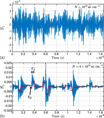
Figure 9: (a) Typical numerical simulations of a time sequence of the two-body spin component $\braket{S_{z}}(t)$ at a low density of $N=10^{12}\,\mathrm{at.cm}^{-3}$, a 2 mW probe power and a detuning $\Delta/2\pi=300\,\mathrm{MHz}$. (b) Simulations for a density $N=4\times 10^{14}\,\mathrm{at.cm}^{-3}$. The step-like red dotted line represents the fluctuations of the steady-state $\braket{S_{z}}^{(st)}$ around which the spins precess.

For this purpose, it is actually helpful to analyze the results in the time domain: figure 9 shows time traces of $\langle S_{z}\rangle(t)$ obtained for two different atomic densities. The plot obtained for $N=10^{12}\,\mathrm{at.cm}^{-3}$ (fig.9 (a)) shows the usual random noise modulated at the Larmor frequency, as expected from the single particle dynamics. However, the results at $N=4\times 10^{14}\,\mathrm{at.cm}^{-3}$, shown in fig.9 (b), is drastically different. In that case, it is clearly visible that each change in the two atoms conformation "triggers" a stochastic precession of the two-body spin coherences $\braket{S_{z}}$, with a random amplitude. This excitation originates from non-adiabatic changes in the two-atom eigenstates induced by the changes in the conformation. In other words, the changes in the dipole-dipole coupling are a source of spin noise itself.

Let alone the transit and optical relaxations, it creates a stochastic dynamics of the density matrix $\displaystyle{\rho(t)=e^{-\frac{i}{\hbar}\int_{0}^{t}\left(H_{0}+V_{dd}(t^{\prime})\right)\mathrm{dt^{\prime}}}\,\rho_{0}\,e^{\frac{i}{\hbar}\int_{0}^{t}\left(H_{0}+V_{dd}(t^{\prime})\right)\mathrm{dt^{\prime}}}}$ where $V_{dd}(t)$ itself is a random operator with a time correlation $\tau_{c}$. The system then evolves at certain frequencies that are specific to the spatial arrangement at a given time $t$. Indeed, one can see in fig.9 (b) that after a change of geometry at an arbitrary time $t=t_{0}$ (indicated in fig. 9(b)), the density matrix evolves towards a new steady-state which depends on the operator $V_{dd}$ at $t_{0}$. Consequently, the spin component $\braket{S_{z}}(t)$ precesses while evolving towards a steady-state value that can be non-zero (e.g. $\langle S_{z}\rangle^{(st)}\simeq 5\times 10^{-3}$ for the change at $t_{0}$). The red dotted-line in fig. (9) (b) shows these step-like fluctuating steady-states. We emphasize here that the value of $\tau_{c}$ has been enlarged to $500\,\mathrm{ns}$ in the simulations to make this mechanism more visible. These slower fluctuations of the spins are related to the two-body correlated dynamics, and do not exist at low densities, where the atoms follow a single-particle equation of evolution.

This variation of the value $\braket{S_{z}}^{(st)}$ around which the spin oscillates is also responsible for the low-frequency noise visible on the experimental spectra in figure 2(b) and the simulated spectra of figure 8(b). Since the spin dynamics is intrinsic to the operator $V_{dd}$ at time t, the steady-state values of $\braket{S_{z}}$ are random, with a zero average over all possible conformation of the two-body system. $\braket{S_{z}}^{(st)}$ is thus a centered random process with a finite correlation time $\tau_{c}$. Since $\braket{S_{z}}(t)$ is at each time evolving towards the steady-state value of the considered conformation, this noise must appear in the spin noise spectrum. Assuming that the noise autocorrelation decreases exponentially, the Wiener-Khinchin theorem states that the corresponding PSD is a Lorentzian line with a HWHM $\gamma_{c}=1/\tau_{c}$. The experimental measurement of $\gamma_{c}/2\pi=14.1\,\mathrm{MHz}$ thus gives an experimental estimation for the binary lifetime of $\tau_{c}=11.2\,\mathrm{ns}$. This value of $\tau_{c}$ is smaller than the one we have used in our simulations (see fig.8): this is due to the way we implement the change of geometry in our simulations, as discussed in details in Appendix C. However, it should be noted that the $100\,\mathrm{ns}$ value used in the simulations yields the correct linewidth for the low-frequency tail, hence the good agreement between the simulated and experimental spectra. Eventually, we proved that the existence of this low-frequency noise is a genuine hallmark of correlated, two-body dynamics. As such, this opens the way to the use of SNS to study possible entanglement created and sustained by dipole-dipole coupling.

It is also remarkable that such a spectral feature allows us to estimate the lifetime of the binary formed by the DDI, and therefore the typical range of the interaction. Since we do not use any buffer gas, the trajectories of the atoms in the cell are essentially ballistic. Consequently, the estimated lifetime $\tau_{c}=11.2\,\mathrm{ns}$ gives an interaction range of $a_{c}^{exp}=\bar{v}\tau_{c}=4.1$ µm. To discuss the meaning of this distance $a_{c}$, it is useful to clearly distinguish it from the other typical distance $r_{0}$ discussed earlier in the paper. Indeed, we have shown that $r_{0}\simeq\lambda/2\pi$ is the typical interatomic distance for which the signatures of the DDI, namely the inhomogeneous broadening and the low-frequency noise, begins to appear of the SN spectra. This suggests that $r_{0}$ sets the scale for which (i) the splitting induced by the DDI exceeds the natural spin noise linewidth; (ii) the two-atom spin component $\langle S_{z}\rangle^{(st)}$ at steady-state may differ significantly from the value it takes for independent atoms. Nevertheless, the low-frequency tail contains an additional information: the typical value of the time $\tau_{c}$ and thus the distance $a_{c}$ over which the dynamics of the atoms stays correlated. We emphasize here that these two length scales $r_{0}$ and $a_{c}$ are different: $r_{0}$ depends on the characteristic ratio between $V_{dd}$ and the single-atom energies and decoherence rates, whereas $a_{c}$ is more intrinsic to the dipole-dipole coupling mechanism itself. In this regard, we expect a dependence of $a_{c}$ on the laser detuning and power: $a_{c}(\Delta,\Omega)$. The present results thus certainly calls for further systematic measurement of these dependencies.

V Conclusion

We have experimentally and theoretically investigated a high-density regime of spin noise spectroscopy in a vapor of natural Rubidium. For that purpose, using a mm-thick vapor cell, we have performed a spectral analysis of the Faraday rotation of a probe light tuned close to the $\mathrm{D_{2}}$ line of Rubidium. Due to the low optical depths allowed by such a thin cell, we were able to probe a regime where the light detuning is small enough to effectively drive dipoles in the ensemble, while the high density allows the atoms to strongly interact. In that case, we have shown that the resonant dipole-dipole interaction taking place in the vapor induces drastic changes in the spin noise spectra compared to the signals at lower temperature. Indeed, the spectra obtained at densities above $N=10^{14}\,\mathrm{at.cm}^{-3}$ exhibit a very broad linewidth, unexplained by the usual single-particle relaxation mechanisms. Moreover, a large asymmetry in the lineshapes reveals the appearance of a broad noise component centered on low frequencies.

To explain such features, we have proposed a microscopic model based on the evolution of a density matrix in a two-particle Hilbert space. We have implemented simulations based on a master equation that includes dipole-dipole coupling as well as radiative and transit relaxations. We have shown that in the case of atoms fixed in the lab frame, the interaction hamiltonian $V_{dd}$ is responsible for a splitting in the spin noise spectrum of the two-body system. We have analytically studied the changes in the eigenfrequencies of the coupled ground-state due to the DDI eventually showing the appearance of new frequencies in the SN spectrum. We then added the atomic motion as fluctuations in the coordinates of the two-atom conformation. Since $V_{dd}$ is highly dependent on the spatial arrangement of the atoms, this results in a broad spin noise peak, coming from the averaging of a set of split spectra. Therefore, the anomalous broadening is actually inhomogeneous and coming from the various atomic conformations, rather than an additional decoherence of the system.

Finally, we proved that including the fluctuations of the conformation of the atoms is responsible for the appearance of the low-frequency noise. We have interpreted this noise as coming from the changes in the eigenstates due to the noise in $V_{dd}$ itself. Consequently, this noise is a signature of the evolution of the two-body system coupled by the DDI, allowing collective spin noise to exist. We have then estimated a DDI interaction range $a_{c}=4.1$ µm from the experimental data, consistent with recent 2D-spectroscopy experiments in Rb vapors Liang and Li (2021); Yu et al. (2019); Falvo and Li (2023); Gao et al. (2016).

This study opens the way to the characterization of collective spin noise in more complex samples, or resulting from other types of long-range interaction. It also opens the possibility to study entanglement using simple SNS setups. Further researches include a thorough statistical description of the noise created by the fluctuations in the dipole-dipole coupling itself. The study of three-body or many-body interactions at higher densities is also an exciting prospect, and may actually already be relevant in the regime presented here. Finally, this study is one step further towards the observation of higher-order correlators in strongly interacting atomic systems.

Appendix A Angular dependence of the SN spectra splitting induced by the DDI

In section III.B, we numerically simulated a set of SN spectra showing the influence of the interatomic distance on the strength of the splitting induced by the DDI. We discussed the power-law scaling of the splitting with the inverse interatomic distance. We ran such simulations for fixed angular coordinates $\theta=0,\,\phi=0$. However, it is clear from the definition of $\overline{\overline{\zeta}}(r_{ij})$, given by eq.(7) of the main text, that the angular coordinates also play a crucial role in the strength of the DDI, as we now discuss.

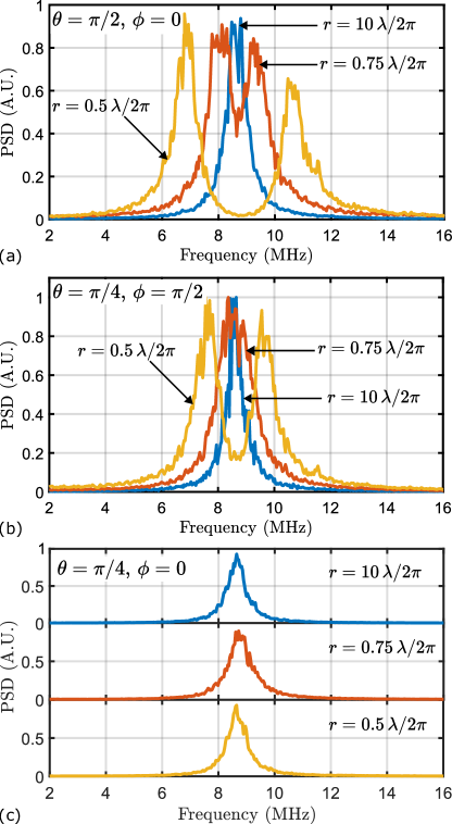
Figure 10: Examples of spin noise spectra obtained for angular coordinates (a) $\theta=\pi/2$, $\phi=0$; (b) $\theta=\pi/4$, $\phi=\pi/2$ and $\theta=\pi/4$, $\phi=0$. For each set of angles, the transition between the weak and strong coupling regime is shown using three interatomic distances. In the last case, no significant modification of the spectrum is induced by the DDI.

We show in figure 10 a few examples of other sets of angular coordinates $\theta,\,\phi$ to show how they affect the splitting of the SN spectra. One can for instance see in fig.10(a) that the choice of $\theta=\pi/2,\phi=0$ leads to a strong splitting, which is of the same order of magnitude as the configuration $\theta=0,\phi=0$ presented and analytically studied in the main text. However, it is much reduced when $\theta=\pi/4,\phi=\pi/2$ (fig 10(b)) and vanishes completely when $\theta=\pi/4$ and $\phi=0$ (fig. 10 (c)).

Understanding this dependence is non trivial without using any numerical simulations. The electromagnetic Green’s dyadic $\displaystyle{\overline{\overline{G}}(\mathbf{r}_{i},\mathbf{r}_{j},\omega_{0})=\quantity(\overline{\overline{1\kern-2.5pt\text{l}}}+\dfrac{\bm{\nabla}\bm{\nabla}}{k^{2}})\dfrac{e^{ik_{0}r_{ij}}}{k_{0}r_{ij}}}$ characterizes the electric field created in space by an oscillating dipole $\mathbf{d}(\mathbf{r}_{1},t)$ according to:

$$\mathbf{E}(\mathbf{r},t)=\dfrac{1}{4\pi\varepsilon_{0}}\overline{\overline{G}}(\mathbf{r},\mathbf{r}_{1},\omega_{0})\cdot\mathbf{d}(\mathbf{r}_{1},t)$$ (17)

The electrostatic energy $\Delta E_{2}=-\left(\mathbf{d_{2}}\right)^{*}\cdot\mathbf{E}(\mathbf{r_{2}},t)$ acquired by the second dipole $\mathbf{d}_{2}$ is thus governed by the elements of the tensor $\overline{\overline{\zeta}}(r_{12})$ discussed in the main text. An explicit expression of the electric field $\mathbf{E}(\mathbf{r},t)$ can be found in electrodynamics and optics textbooks Jackson (2009); Griffiths (2023). It can be separated in three contribution: the quasi-static (near-field) term, dominating for $kr\ll 1$, the radiated (far-field) term ($kr\gg 1$) and finally the inductive term ($kr\simeq 1$).

The near and far-field terms are well known, so that one can somehow have a view of which coupling $\zeta_{\lambda,\lambda^{\prime}}$ will be non zero by looking at the characteristic field lines in these regime. Unfortunately, they are not relevant in the study presented here for two reasons: (i) the DDI mediated by the far field is very weak, and the associated perturbation of the two-body ground-state cannot be seen experimentally; (ii) the DDI in the near-field is relevant for atomic densities higher than what we can achieve experimentally. Therefore, the relevant interacting regime in the experimental results presented here is closer to $kr\leq 1$, which does not allow for straightforward representation of the electric field, and thus of the shape and strength of the electromagnetic Green’s tensor.

Appendix B Perturbation of the two-atom ground-states via an exchange of atomic excitation

Here we give more details about the terms in the expression of $V_{dd}$

$$V_{dd}=\hbar\sum_{\begin{subarray}{c}i\neq j\\ \lambda,\lambda^{\prime}\end{subarray}}\zeta_{\lambda,\lambda^{\prime}}(r_{ij})\frac{D_{+}^{\lambda,i}D_{-}^{\lambda^{\prime},j}}{d_{0}^{2}}$$ (18)

that are relevant to compute the first-order perturbation of the two-atom ground-state by ddi. As discussed in the text, we consider the case where the light is $\sigma$-polarized. The action of the Hamiltonian $V_{dd}$ is to describe the de-excitation of an atom and the excitation of its neighbour via an exchange of light. Since we built the two-body lower manifold using the one-body eigenstates of the Zeeman and light-matter coupling Hamiltonian, these states have a non-zero dipole. Such a situation is depicted in fig. 11, where each one-body atomic state is schematized as a superposition of a ground-state sublevel (large dot) and an excited-state sublevel (small dot).

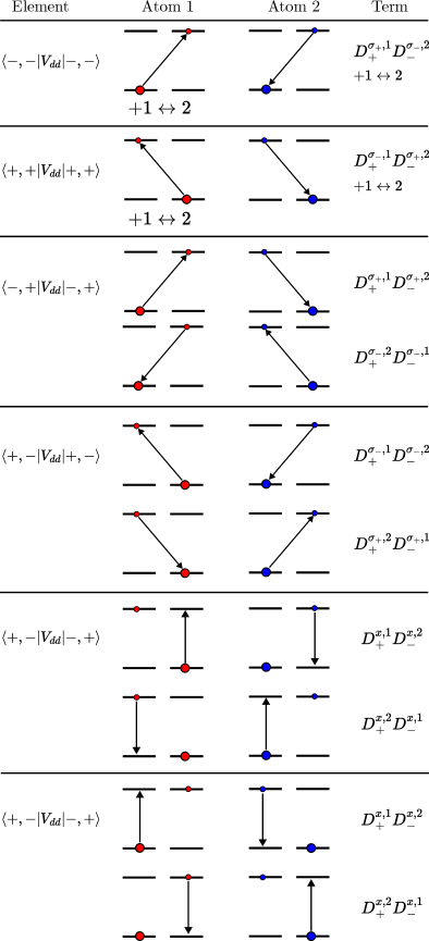
Figure 11: Schematics of the relevant operators in the calculation the first-order energy shifts experienced by the two-body ground-states under the action of the ddi. An upward (downward) arrow designates the action of a $D_{+}^{i}\,(D_{-}^{i})$ operator on the atom $i$.

The relevant operators in the right-hand side sum of eq.(18) are the ones showing non-zero diagonal matrix element for the four states composing the two-body lower manifold: $\{\ket{-,-},\ket{-,+},\ket{+,-},\ket{+,+}\}$. These terms are summarized in fig.11, where the corresponding product of dipole operators is expressed in the $\{x,\,\sigma_{+},\,\sigma_{-}\}$ basis, which is the most convenient to describe the excitation and de-excitation of atoms. In the single-atom basis $\{\ket{g,-1/2},\,\ket{g,+1/2},\,\ket{e,-1/2},\,\ket{e,+1/2}\}$, we have:

$$\begin{split}D_{+}^{x}=\dfrac{d_{0}}{\sqrt{3}}\begin{pmatrix}0&0&0&0\\ 0&0&0&0\\ -1&0&0&0\\ 0&1&0&0\end{pmatrix},\\ D_{+}^{\sigma_{+}}=\sqrt{\dfrac{2}{3}}d_{0}\begin{pmatrix}0&0&0&0\\ 0&0&0&0\\ 0&0&0&0\\ -1&0&0&0\end{pmatrix},\\ D_{+}^{\sigma_{-}}=\sqrt{\dfrac{2}{3}}d_{0}\begin{pmatrix}0&0&0&0\\ 0&0&0&0\\ 0&-1&0&0\\ 0&0&0&0\end{pmatrix},\end{split}$$ (19)

and obviously $D_{-}^{x}=(D_{+}^{x})^{\dagger}$, $D_{-}^{\sigma_{+}}=(D_{+}^{\sigma_{-}})^{\dagger}$ and $D_{-}^{\sigma_{-}}=(D_{+}^{\sigma_{+}})^{\dagger}$. Keeping in mind that for the case $\theta=0,\phi=0$, $\overline{\overline{\zeta}}(r_{ij})$ is diagonal in the $\{x,y,z\}$ basis, one can then use the simple expression of $V_{dd}$ given in the main text by eq. (11), substitute the dipole operators in the $\{x,y,z\}$ basis by the ones listed above, and keep only the terms depicted in figure 11.

Consider first the state $\ket{-,-}$: the operators $O$ in the right-hand side of eq. (18) with non-zero matrix elements $\braket{-,-}{O}{-,-}$ correspond to an excitation of the first atom by a $\sigma_{+}$-polarized light emitted by the de-excitation of the second atom. Similarly, the state $\ket{+,+}$ is only perturbed at first-order by the same mechanism, except that the emitted light should be $\sigma_{-}$-polarized. For these mechanisms, the two additional operators obtained by the exchange between atom 1 and 2 must also be considered. This gives the same shift for both states $\ket{-,-}$ and $\ket{+,+}$:

$$\braket{-,-}{V_{dd}}{-,-}=\braket{+,+}{V_{dd}}{+,+}=\alpha(\zeta_{yy}+\zeta_{zz})$$ (20)

where, letting aside the CG coefficients which are intrinsic to the atomic structure we consider, $\alpha=\dfrac{\Omega^{2}\Delta^{2}/4}{(\Omega^{2}/4+\Delta^{2})^{2}}$.

The case of the two other states $\ket{+,-}$ and $\ket{-,+}$ is peculiar due to their initial degeneracy. The associated diagonal terms in $V_{dd}$ involve an excitation and de-excitation sequence with radiations of opposite polarizations, as seen in fig. 11. Moreover, they are coupled to one another by the absorption and emission process with $x$ polarization, that played no role earlier for the $\ket{-,-}$ and $\ket{+,+}$ states. One can show that in the reduced basis $\{\ket{-,+},\,\ket{+,-}\}$, $V_{dd}$ reads:

$$V_{dd}=\begin{pmatrix}\zeta_{yy}-\zeta_{zz}&2\zeta_{xx}\\ 2\zeta_{xx}&\zeta_{yy}-\zeta_{zz}.\end{pmatrix}$$ (21)

The diagonalization of $V_{dd}$ in this subspace then yields the two symmetrized states $\ket{s}=\dfrac{\ket{+,-}+\ket{-,+}}{\sqrt{2}}$ and $\ket{u}=\dfrac{\ket{+,-}-\ket{-,+}}{\sqrt{2}}$ with respective energy shifts

$$\left\{\begin{array}[]{c c l}\braket{s}{V_{dd}}{s}&=&\alpha(\zeta_{yy}-\zeta_{zz}+2\zeta_{xx}),\\ \braket{u}{V_{dd}}{u}&=&\alpha(\zeta_{yy}-\zeta_{zz}-2\zeta_{xx}),\\ \end{array}\right.$$ (22)

hence the result of eq. (13) in the main text.

Appendix C Numerical implementation of the two-atom geometry changes and corresponding autocorrelation function

We discuss here the choice of the geometry correlation time $\tau_{c}$ we used in the numerical simulations to reproduce the experimental data. Indeed, to simulate the finite lifetime of the binary formed by the DDI, we assume in our model that the interatomic coordinates triplet $(r,\,\theta,\,\phi)$ randomly changes after each period of duration $\tau_{c}$. This results in step-like changes in the steady-state $z$-component of the spin $\langle S_{z}\rangle^{(st)}$, with random amplitudes. Consequently, the autocorrelation function of the stationary random variable $\langle S_{z}\rangle^{(st)}$ is triangular:

$$\overline{\langle S_{z}\rangle^{(st)}(t)\langle S_{z}\rangle^{(st)}(0)}\ \propto\left\{\begin{array}[]{l r}1-|t|/\tau_{c}&\mathrm{for}\,|t|\leq\tau_{c},\\ 0&\mathrm{otherwise}.\end{array}\right.$$ (23)

Using the Wiener-Kinchin theorem, the Fourier Transform of this function gives the associated PSD $C_{zz}(\nu)$, which corresponds to the low-frequency tail of the high-density SN spectra. It gives:

$$C_{zz}(\nu)=\sigma^{2}_{\langle S_{z}\rangle^{(st)}}\mathrm{sinc}^{2}\left(\pi\tau_{c}/\nu\right),$$ (24)

with $\sigma^{2}_{\langle S_{z}\rangle^{(st)}}$ the variance of $\langle S_{z}\rangle^{(st)}$ and the convention $\mathrm{sinc}(\nu)=\sin(\nu)/\nu$.

Consequently, the low-frequency tail appearing in our simulations (see fig.8 (b) for instance) is sinc-shaped: it shows a first zero for $\nu=1/\tau_{c}$ and a first ripple for $\nu=3/2\tau_{c}$. Higher-order ripples are hidden in the noise due to the finite number of samples used to compute the numerical spectra. Taking a correlation time $\tau_{c}=100\,\mathrm{ns}$, this gives a first zero at $\nu=10\,\mathrm{MHz}$ and a first ripple centered on $\nu=15\,\mathrm{MHz}$. These values are consistent with the experimental estimation of the low-frequency noise linewidth in fig.4: $\gamma_{c}/2\pi=14.1\pm 0.8\,\mathrm{MHz}$, hence the agreement in the lineshapes between simulations and experiments.

However, one must keep in mind that this sinc-shape is only a consequence of our choice to change randomly the two-body conformation after each step of duration $\tau_{c}$. Nevertheless, it is physically more reasonable to assume an exponential decay for the binary in the experiment. The value of $\gamma_{c}$ then yields an experimental lifetime $\tau_{c}=1/\gamma_{c}=11.2\,\mathrm{ns}$ as discussed in the main text.

References

- Aleksandrov and Zapasskii (1981) E. B. Aleksandrov and V. S. Zapasskii, JETP 54 (1981).
- Crooker et al. (2004) S. A. Crooker, D. G. Rickel, A. V. Balatsky, and D. L. Smith, Nature 431, 49 (2004), number: 7004 Publisher: Nature Publishing Group.
- Katsoprinakis et al. (2007) G. E. Katsoprinakis, A. T. Dellis, and I. K. Kominis, Physical Review A 75, 042502 (2007).
- Mihaila et al. (2006) B. Mihaila, S. A. Crooker, D. G. Rickel, K. B. Blagoev, P. B. Littlewood, and D. L. Smith, Physical Review A 74, 043819 (2006).
- Fomin et al. (2020) A. A. Fomin, M. Y. Petrov, G. G. Kozlov, M. M. Glazov, I. I. Ryzhov, M. V. Balabas, and V. S. Zapasskii, Physical Review Research 2, 012008 (2020).
- Liu et al. (2022) S. Liu, P. Neveu, J. Delpy, L. Hemmen, E. Brion, E. Wu, F. Bretenaker, and F. Goldfarb, New Journal of Physics 24, 113047 (2022).
- Liu et al. (2023) S. Liu, P. Neveu, J. Delpy, E. Wu, F. Bretenaker, and F. Goldfarb, Physical Review A 107, 023527 (2023), publisher: American Physical Society.
- Hübner et al. (2014) J. Hübner, F. Berski, R. Dahbashi, and M. Oestreich, physica status solidi (b) 251, 1824 (2014).
- Poltavtsev et al. (2014) S. V. Poltavtsev, I. I. Ryzhov, M. M. Glazov, G. G. Kozlov, V. S. Zapasskii, A. V. Kavokin, P. G. Lagoudakis, D. S. Smirnov, and E. L. Ivchenko, Physical Review B 89, 081304 (2014).
- Crooker et al. (2010) S. A. Crooker, J. Brandt, C. Sandfort, A. Greilich, D. R. Yakovlev, D. Reuter, A. D. Wieck, and M. Bayer, Physical Review Letters 104, 036601 (2010).
- Glasenapp et al. (2016) P. Glasenapp, D. S. Smirnov, A. Greilich, J. Hackmann, M. M. Glazov, F. B. Anders, and M. Bayer, Physical Review B 93, 205429 (2016).
- Gundín et al. (2024) M. Gundín, P. Hilaire, C. Millet, E. Mehdi, C. Antón, A. Harouri, A. Lemaître, I. Sagnes, N. Somaschi, O. Krebs, P. Senellart, and L. Lanco, “Spin Noise Spectroscopy of a Single Spin using Single Detected Photons,” (2024).
- Zapasskii et al. (2013) V. S. Zapasskii, A. Greilich, S. A. Crooker, Y. Li, G. G. Kozlov, D. R. Yakovlev, D. Reuter, A. D. Wieck, and M. Bayer, Physical Review Letters 110, 176601 (2013).
- Swar et al. (2021) M. Swar, D. Roy, S. Bhar, S. Roy, and S. Chaudhuri, Physical Review Research 3, 043171 (2021).
- Glasenapp et al. (2014) P. Glasenapp, N. Sinitsyn, L. Yang, D. Rickel, D. Roy, A. Greilich, M. Bayer, and S. Crooker, Physical Review Letters 113, 156601 (2014).
- Chalupczak and Godun (2011) W. Chalupczak and R. M. Godun, Physical Review A 83, 032512 (2011).
- Horn et al. (2011) H. Horn, G. M. Müller, E. M. Rasel, L. Santos, J. Hübner, and M. Oestreich, Physical Review A 84, 043851 (2011), publisher: American Physical Society.
- Swar et al. (2018) M. Swar, D. Roy, D. D, S. Chaudhuri, S. Roy, and H. Ramachandran, Optics Express 26, 32168 (2018).
- Sinitsyn and Pershin (2016) N. A. Sinitsyn and Y. V. Pershin, Reports on Progress in Physics 79, 106501 (2016).
- Li et al. (2013) F. Li, Y. V. Pershin, V. A. Slipko, and N. A. Sinitsyn, Physical Review Letters 111, 067201 (2013).
- Delpy et al. (2023a) J. Delpy, S. Liu, P. Neveu, C. Roussy, T. Jolicoeur, F. Bretenaker, and F. Goldfarb, New Journal of Physics 25, 093055 (2023a).
- Li et al. (2016) F. Li, S. A. Crooker, and N. A. Sinitsyn, Physical Review A 93, 033814 (2016).
- Mouloudakis et al. (2022) K. Mouloudakis, G. Vasilakis, V. G. Lucivero, J. Kong, I. K. Kominis, and M. W. Mitchell, Physical Review A 106, 023112 (2022).
- Mouloudakis et al. (2019) K. Mouloudakis, M. Loulakis, and I. K. Kominis, Physical Review Research 1, 033017 (2019).
- Dellis et al. (2014) A. T. Dellis, M. Loulakis, and I. K. Kominis, Physical Review A 90, 032705 (2014).
- Roy et al. (2015) D. Roy, L. Yang, S. A. Crooker, and N. A. Sinitsyn, Scientific Reports 5, 9573 (2015), publisher: Nature Publishing Group.
- Mouloudakis and Kominis (2021) K. Mouloudakis and I. K. Kominis, Physical Review A 103, L010401 (2021).
- Gross and Haroche (1982) M. Gross and S. Haroche, Physics Reports 93, 301 (1982).
- Röhlsberger et al. (2010) R. Röhlsberger, K. Schlage, B. Sahoo, S. Couet, and R. Rüffer, Science 328, 1248 (2010).
- Keaveney et al. (2012) J. Keaveney, A. Sargsyan, U. Krohn, I. G. Hughes, D. Sarkisyan, and C. S. Adams, Physical Review Letters 108, 173601 (2012), publisher: American Physical Society.
- Peyrot et al. (2019) T. Peyrot, Y. Sortais, J.-J. Greffet, A. Browaeys, A. Sargsyan, J. Keaveney, I. Hughes, and C. Adams, Physical Review Letters 122, 113401 (2019), publisher: American Physical Society.
- Lewis (1980) E. L. Lewis, Physics Reports 58, 1 (1980).
- Browaeys et al. (2016) A. Browaeys, D. Barredo, and T. Lahaye, Journal of Physics B: Atomic, Molecular and Optical Physics 49, 152001 (2016).
- Browaeys and Lahaye (2020) A. Browaeys and T. Lahaye, Nature Physics 16, 132 (2020), number: 2 Publisher: Nature Publishing Group.
- Delpy et al. (2024) J. Delpy, N. Fayard, F. Bretenaker, and F. Goldfarb, submitted (2024).
- Weller et al. (2011) L. Weller, R. J. Bettles, P. Siddons, C. S. Adams, and I. G. Hughes, Journal of Physics B: Atomic, Molecular and Optical Physics 44, 195006 (2011).
- Glazov and Zapasskii (2015) M. M. Glazov and V. S. Zapasskii, Optics Express 23, 11713 (2015).
- Chandrasekhar (1943) S. Chandrasekhar, Reviews of Modern Physics 15, 1 (1943), publisher: American Physical Society.
- Lehmberg (1970) R. H. Lehmberg, Physical Review A 2, 883 (1970).
- Agarwal (2012) G. S. Agarwal, “Quantum optics,” (2012), iSBN: 9781139035170 Publisher: Cambridge University Press.
- Le Kien and Rauschenbeutel (2017) F. Le Kien and A. Rauschenbeutel, Physical Review A 95, 023838 (2017), publisher: American Physical Society.
- Reitz et al. (2022) M. Reitz, C. Sommer, and C. Genes, PRX Quantum 3, 010201 (2022).
- Delpy et al. (2023b) J. Delpy, S. Liu, P. Neveu, E. Wu, F. Bretenaker, and F. Goldfarb, Physical Review A 107, L011701 (2023b), publisher: American Physical Society.
- Happer (1970) W. Happer, Progress in Quantum Electronics 1, 51 (1970).
- Liang and Li (2021) D. Liang and H. Li, The Journal of Chemical Physics 154, 214301 (2021).
- Yu et al. (2019) S. Yu, M. Titze, Y. Zhu, X. Liu, and H. Li, Optics Express 27, 28891 (2019), publisher: Optica Publishing Group.
- Falvo and Li (2023) C. Falvo and H. Li, The Journal of Chemical Physics 159, 064304 (2023).
- Gao et al. (2016) F. Gao, S. T. Cundiff, and H. Li, Optics Letters 41, 2954 (2016), publisher: Optica Publishing Group.
- Jackson (2009) J. D. Jackson, Classical electrodynamics, 3rd ed. (Wiley, Hoboken, NY, 2009).
- Griffiths (2023) D. J. Griffiths, Introduction to Electrodynamics, 5th ed. (Cambridge University Press, 2023).