$W-$mass and Muon $g-2$ in Inert 2HDM Extended by Singlet Complex Scalar

Abstract

The deviations of the recent measurements of the muon magnetic moment and the $W-$boson mass from their SM predictions hint to new physics beyond the SM. In this article, we address the observed discrepancies in the $W$-boson mass and muon anomalous magnetic moment in the Inert Two Higgs Doublet Model (I2HDM) extended by a complex scalar field singlet under the SM gauge group. The model is constrained from the existing LEP data and the measurements of partial decay widths to gauge bosons at LHC. It is shown that a large subset of this constrained parameter space of the model can simultaneously accommodate the $W$-boson mass and also explain the muon $g-2$ anomaly.

I Introduction

The departures of low-energy observables from their Standard Model (SM) predictions can provide indirect clues for physics beyond the SM. The $W$ boson mass and the anomalous magnetic moment of muon are two such most notable anomalies that provide a stringent test of the SM Crivellin and Mellado (2023) and should be explained by any proposed model beyond SM.

The CDF Collaboration has reported a notable discrepancy between the measured and predicted values of $W$ mass through a series of increasingly precise measurements Kotwal (2024). The most recent measurement by CDF collaboration Aaltonen et al. (2022)

$$m_{{}_{W}}^{\rm CDF}=(80.4335\pm 0.0094)\,{\text{GeV}}$$ (1)

on their full Run-2 dataset of 8.8 fb^-1 which deviates from the global average of the other experiments Workman et al. (2022)

$$m_{{}_{W}}^{\rm PDG}=(80.377\pm 0.012)\,{\text{GeV}}.$$ (2)

and also the recent improved measurement by ATLAS Aad et al. (2024) which is $m_{{}_{W}}^{\rm ATLAS}=(80.3665\pm 0.0159)\,$GeV. The global fit SM prediction Workman et al. (2022) ($80.356\pm 0.006$) GeV is about $7\sigma$ below the value reported by CDF.

A more recent global fit SM prediction reported by reference de Blas et al. (2022)

$$m_{{}_{W}}^{\rm SM}=(80.3499\pm 0.0056)\,{\text{GeV}}$$ (3)

further increases the discrepancy from CDF value. Such a significant discrepancy, calls for a thorough investigation of physics beyond the Standard Model (BSM) Kotwal (2024).

Another long standing discrepancy is in the muon anomalous magnetic moment where the direct measurements of muon ($g-2$) are precisely made and have been confirmed in several experiments. The most recent measurement of the anomalous muon magnetic moment by the Fermilab Muon $g-2$ Experiment Aguillard et al. (2023) using data collected in 2019 and 2020 gives

$$a_{\mu} = \frac{(g-2)_{\mu}}{2}=116592057(25)\times 10^{-11}(0.21\,\text{ppm})$$

resulting in the new world average

$$a_{\mu}^{\rm exp}=116592059(22)\times 10^{-11}(0.19\,\text{ppm})$$ (5)

The SM prediction is given by et al. (2020)

$$a_{\mu}^{\rm SM} = 116591810(43)\times 10^{-11}$$ (6)

amounting to about $5\sigma$ discrepancy

$$\Delta a_{\mu} = a_{\mu}^{\rm exp}-a_{\mu}^{\rm SM}=\left(2.49\pm 0.48\right)\times 10^{-9}.$$ (7)

This SM prediction uses the conservative leading order data-driven computation of Hadronic Vacuum Polarisation (HVP) Keshavarzi et al. (2020) based on the available data sets for the $e^{+}e^{-}\to$hadrons cross section and the techniques applied for the evaluation of the HVP dispersive integral. The prospects for improvements of the uncertainties in the SM prediction Ignatov et al. (2023); Blum et al. (2023); et al. (2020) may make the SM prediction closer to experimental measurements. However, how would this discrepancy play out by future analysis is not yet settled.

The additional quantum corrections induced by new particles in a model beyond SM might account for the observed anomaly in the $W-$boson mass as well as the muon magnetic moment. These twin problems have been addressed recently in many models beyond the SM Cici and Dag (2024); *Zhu:2023qyt; *Davoudiasl:2023cnc; *Abdallah:2023pbl; *Ahmadvand:2023gse; *Chakrabarty:2022gqi; *Abdallah:2022shy; *Kim:2022axk; *Zheng:2022ssr; *Chakrabarty:2022voz; *Kawamura:2022fhm; *Chowdhury:2022dps; *He:2022zjz; *Kim:2022xuo; *Botella:2022rte; *Bhaskar:2022vgk; *Arcadi:2022dmt; *Kawamura:2022uft; *Zhou:2022cql; *Athron:2022qpo; *Babu:2022pdn; *Bagnaschi:2022qhb with varying degrees of success.

In an earlier work Bharadwaj et al. (2021), the authors have addressed the observed discrepancies in the anomalous magnetic moment of muons and electrons by I2HDM to include a complex scalar field and a charged singlet vector-like lepton. In this spirit we revisit our earlier model albeit without the introduction of a charged vector-like lepton and discuss the constraints on the model parameters from the LEP data and recent Higgs decay data. Using this constrained model, we attempt to address the possibility of explaining such high value of $m_{W}$ as well as an upward pull for muon $g-2$.

The rest of this article is organised as follows: The section II briefly reviews our model. In section III, we discuss the constraints on model parameters coming from the Higgs decay and the LEP data. The additional contributions to muon anomalous magnetic moment and $W-$mass in our model are discussed in section IV and the corresponding numerical results of the regions in parameter space that simultaneously explains both anomalies are given in section V. We summarise our results in the last section VI.

II The model

The I2HDM consiss of two $SU(2)_{L}$ doublets of complex scalar fields: SM-like doublet $\Phi_{1}$ and another doublet $\Phi_{2}$(the inert doublet) possessing the same quantum numbers as $\Phi_{1}$ but with no direct coupling to fermions. We consider a model with the scalar sector of I2HDM extended by a neutral complex gauge singlet scalar field $\Phi_{3}$. After electroweak symmetry breaking (EWSB), $\Phi_{1}$ as well as $\Phi_{3}$ acquire nonzero real vacuum expectation values, $v_{{}_{\!\rm SM}}$ and $v_{s}$ respectively. We invoke a $Z_{2}$ symmetry under which all SM fields and $\Phi_{1}$ are even. The inert doublet fields $\Phi_{2}$ and the singlet scalar $\Phi_{3}$ are odd under this $Z_{2}$ symmetry. Due to this symmetry the scalar fields in $\Phi_{2}$ do not mix with the SM-like field from $\Phi_{1}$. The $Z_{2}$ symmetry also ensures that the SM gauge bosons and fermions are forbidden to have direct interaction with the inert doublet and additional complex scalar singlet. We however, allow an explicit breaking of $Z_{2}$ symmetry in the Yukawa Lagrangian ${\cal L}_{Y}$ in order to facilitate coupling of SM leptons with $CP$ odd pseudo-scalars.

The part of the Lagrangian different from SM Lagrangian is written as

$${\cal L} \supset {\cal L}_{\rm scalar}\ +\ {\cal L}_{Y}\$$ (8a)

$${\cal L}_{\rm scalar} = \left(D_{\mu}\Phi_{1}\right)^{\dagger}\ \left(D^{\mu}\Phi_{1}\right)\ +\ \left(D_{\mu}\Phi_{2}\right)^{\dagger}\ \left(D_{\mu}\Phi_{2}\right)\ +\ \left(D_{\mu}\Phi_{3}\right)^{*}\ \left(D_{\mu}\Phi_{3}\right)\ -\ V_{\rm scalar}$$ (8b)

$$V_{\rm scalar} = V_{\rm 2HDM}\left(\Phi_{1},\Phi_{2}\right)+V_{\rm Singlet}\left(\Phi_{3}\right)+V_{\rm Mix}\left(\Phi_{1},\Phi_{2},\Phi_{3}\right)$$ (8c)

$$= -\frac{1}{2}m_{11}^{2}\left(\Phi_{1}^{\dagger}\Phi_{1}\right)-\frac{1}{2}m_{22}^{2}\left(\Phi_{2}^{\dagger}\Phi_{2}\right)+\frac{\lambda_{1}}{2}\left(\Phi_{1}^{\dagger}\Phi_{1}\right)^{2}+\frac{\lambda_{2}}{2}\left(\Phi_{2}^{\dagger}\Phi_{2}\right)^{2}$$

$$+\lambda_{3}\left(\Phi_{1}^{\dagger}\Phi_{1}\right)\left(\Phi_{2}^{\dagger}\Phi_{2}\right)+\lambda_{4}\left(\Phi_{1}^{\dagger}\Phi_{2}\right)\left(\Phi_{2}^{\dagger}\Phi_{1}\right)+\frac{1}{2}\left[\lambda_{5}\ \left(\Phi_{1}^{\dagger}\Phi_{2}\right)^{2}+\ h.c.\right]$$

$$-\frac{1}{2}m_{33}^{2}\ \Phi_{3}^{*}\Phi_{3}+\frac{\lambda_{8}}{2}\left(\Phi_{3}^{*}\Phi_{3}\right)^{2}+\lambda_{11}\left|\Phi_{1}\right|^{2}\Phi_{3}^{*}\Phi_{3}+\lambda_{13}\left|\Phi_{2}\right|^{2}\Phi_{3}^{*}\Phi_{3}$$

$$-i\,\kappa\,\,\left[\left(\Phi_{1}^{\dagger}\Phi_{2}+\Phi_{2}^{\dagger}\Phi_{1}\right)\,\,\left(\Phi_{3}-\Phi_{3}^{\star}\right)\right]$$

where

$$\Phi_{1}\equiv\left[\begin{array}[]{c}\phi_{1}^{+}\\ \frac{1}{\sqrt{2}}\,\left(v_{\rm SM}+\phi_{1}^{0}+i\,\eta_{1}^{0}\right)\\ \end{array}\right];\,\,\,\Phi_{2}\equiv\left[\begin{array}[]{c}\phi_{2}^{+}\\ \frac{1}{\sqrt{2}}\,\left(\phi_{2}^{0}+i\,\eta_{2}^{0}\right)\\ \end{array}\right]\,\,\,{\rm and}\,\Phi_{3}\equiv\frac{1}{\sqrt{2}}\,\left(v_{s}+\phi_{3}^{0}+i\,\eta_{3}^{0}\right)$$ (8h)

$$-{\cal L}_{\rm Y} = y_{u}\ \overline{Q_{L}}\ \widetilde{\Phi_{1}}\ u_{R}\ +\ y_{d}\ \overline{Q_{L}}\ \Phi_{1}\ d_{R}\ +\ y_{{}_{l}}\ \overline{l_{L}}\ \Phi_{1}\ e_{R}\ +y_{1}\ \overline{l_{L}}\ \Phi_{2}\ e_{R}+\ \text{h.c.}$$ (8i)

where all couplings in the scalar potential and Yukawa sector are real in order to preserve the CP invariance. Here, we have invoked an additional global $U(1)$ symmetry under $\Phi_{3}\to e^{i\,\alpha}\Phi_{3}$ to reduce the number of free parameters in the scalar potential, which is however allowed to be softly broken by the $\kappa$ term.

The stability of the Lagrangian given in (8c) have been discussed in the article Bharadwaj et al. (2021) and we refer the reader to this reference for the co-positivity conditions on the scalar potential and its minimisation.

The absence of mixing among the imaginary component of the inert doublet with the real component of either the first SM like doublet or the singlet results in the decoupling of the mass matrices for neutral scalars and pseudoscalars. The $2\times 2$ CP-even neutral scalar mass matrix arises due to the mixing of the real components of SM like first doublet $\Phi_{1}$ and the singlet $\Phi_{3}$. Diagonalisation of this CP-even mass matrix by orthogonal rotation matrix parameterized in terms of the mixing angle $\theta_{13}$ gives the two mass eigenstates $h_{1}$ and $h_{3}$. with masses given by

$$m_{h_{1}}^{2} = \cos^{2}{\theta_{13}}\,\,\lambda_{1}\,v_{{}_{\!\rm SM}}^{2}+\sin\left(2{\theta_{13}}\right)v_{s}\,\,\lambda_{11}\,\,v_{{}_{\!\rm SM}}$$ (9a)

$$+\sin^{2}{\theta_{13}}\,\,v_{s}^{2}\,\,\lambda_{8}$$

$$m_{h_{3}}^{2} = \sin^{2}{\theta_{13}}\,\,\lambda_{1}\,\,v_{{}_{\!\rm SM}}^{2}-\sin\left(2{\theta_{13}}\right)v_{s}\,\,\lambda_{11}\,\,v_{{}_{\!\rm SM}}$$ (9b)

$$+\cos^{2}{\theta_{13}}\,\,v_{s}^{2}\,\,\lambda_{8}$$

with

$$\tan 2\theta_{13} = \frac{\lambda_{11}\,v_{{}_{\!\rm SM}}v_{s}}{\lambda_{1}\,v_{{}_{\!\rm SM}}^{2}-\lambda_{8}v_{s}^{2}}$$ (9c)

Similarly, the diagonalisation of mass matrix for CP-odd scalars $\eta_{2}^{0}$ and $\eta_{3}^{0}$ gives the pseudoscalar mass eigenstates $A^{0}$ and $P^{0}$ with masses given by

$$m_{A^{0}}^{2} = \frac{1}{2}\left(\overline{\lambda}_{345}\,v_{{}_{\!\rm SM}}^{2}-m_{22}^{2}+\lambda_{13}v_{s}^{2}\right)\cos^{2}\theta_{23}$$ (10a)

$$-\sqrt{2}\kappa\,v_{{}_{\!\rm SM}}\sin 2\theta_{23}$$

$$m_{P^{0}}^{2} = \frac{1}{2}\left(\overline{\lambda}_{345}\,v_{{}_{\!\rm SM}}^{2}-m_{22}^{2}+\lambda_{13}v_{s}^{2}\right)\sin^{2}\theta_{23}$$ (10b)

$$+\sqrt{2}\kappa\,v_{{}_{\!\rm SM}}\sin 2\theta_{23}$$

where $$\overline{\lambda}_{345}=\lambda_{3}+\lambda_{4}-\lambda_{5} \theta_{23}$$ and the mixing angle is given by

$$\kappa=-\,\frac{1}{2\,\sqrt{2}\,v_{{}_{\!\rm SM}}}\left(m^{2}_{P^{0}}+m^{2}_{A^{0}}\right)\tan\left(2\,\theta_{23}\right)$$ (10c)

Out of the remaining neutral and charged scalar mass eigenstates, $\eta_{1}^{0}$ and $\phi_{1}^{\pm}$ are the massless Nambu-Golsdstone bosons and the masses of $\phi_{2}^{0}$ and $\phi_{2}^{\pm}$ which are renamed as $h_{2}$ and $H^{\pm}$ respectively are given by

$$m_{h_{2}}^{2} = \frac{1}{2}\ \left[-m_{22}^{2}+\ \left(\lambda_{3}+\lambda_{4}+\lambda_{5}\right)\,v_{{}_{\!\rm SM}}^{2}+\lambda_{13}v_{s}^{2}\right]$$

$$m_{H^{\pm}}^{2} = -m_{22}^{2}\ +\lambda_{3}v_{{}_{\!\rm SM}}^{2}+\ \lambda_{13}v_{s}^{2}$$ (11b)

The twelve independent parameters in the scalar potential (8c), namely, $m_{11}$, $m_{22}$, $m_{33}$, $\lambda_{i=1,\,\ldots\,5}$, $\lambda_{8}$, $\lambda_{11}$, $\lambda_{13}$ and $\kappa$ can now be expressed in terms of the following physical masses and mixing angles:

$$v_{{}_{\!\rm SM}},\,v_{s},\,m_{h_{1}}^{2},\,m_{h_{2}}^{2},\,m_{h_{3}}^{2},\,m_{H^{\pm}}^{2},\,\ m_{A^{0}}^{2},\,m_{P^{0}}^{2},\,\theta_{13},\,\theta_{23},\,m_{22}^{2}$$

(12)

For the relations among the mass parameters and scalar couplings of the Lagrangian, reader is referred to the appendix A of reference Bharadwaj et al. (2021)). Further, the dimension-full scalar triple couplings of the charged Higgs bosons with neutral scalars are expressed as $g_{h_{i}H^{+}H^{-}}=(\lambda_{h_{i}H^{+}H^{-}}\,v_{{}_{\!\rm SM}})$, where

$$\lambda_{h_{1}H^{+}H^{-}} = \lambda_{3}\,\cos\theta_{13}+\frac{v_{s}}{v_{{}_{\!\rm SM}}}\,\lambda_{13}\,\sin\theta_{13}$$ (13a)

$$\lambda_{h_{3}H^{+}H^{-}} = \frac{v_{s}}{v_{{}_{\!\rm SM}}}\lambda_{13}\cos\theta_{13}\ -\ \lambda_{3}\ \sin\theta_{13}$$ (13b)

The Yukawa interactions given in (8i) can be re-written in terms of mass eigenstates as

$$-{\cal L}^{{}^{\rm Yukawa}}_{\rm SM\,Fermions} = \sum_{s_{i}\equiv h_{1},h_{3}}\frac{y_{{}_{ffs_{i}}}}{\sqrt{2}}\left(v_{{}_{\!\rm SM}}\,\,\delta_{s_{i},h_{1}}+s_{i}\right)\bar{f}\ f\ +\frac{y_{{}_{llh_{2}}}}{\sqrt{2}}(h_{2}\ \bar{l}^{-}\ l^{-})+\sum_{s_{i}\equiv P^{0},A^{0}}\frac{y_{{}_{lls_{i}}}}{\sqrt{2}}(s_{i}\ \bar{l}^{-}\gamma_{5}\ l^{-})$$ (14)

$$+\ \left[y_{{}_{l\nu H^{-}}}\ (\bar{\nu}_{l}\ P_{R}\ l^{-}H^{+})+{\rm h.c.}\right],$$

where $f$ and $l^{-}$ represent SM fermions and SM charged leptons respectively. The Yukawa couplings with scalar/ pseudoscalar mass eigenstates are listed in table 1.

$y_{{}_{ffh_{1}}}\,\,\,$	$\quad\left(\sqrt{2}m_{f}/v_{\rm SM}\right)\cos\theta_{13}$	$\,y_{{}_{llh_{2}}}\,\,\,$	$y_{1}$
$y_{{}_{ffh_{3}}}\,\,\,$	$-\left(\sqrt{2}m_{f}/v_{\rm SM}\right)\sin\theta_{13}$	$\,y_{{}_{llP^{0}}}\,\,\,$	$-i\ y_{1}\sin\theta_{23}$
$y_{{}_{l\nu H^{-}}}$	$y_{1}$	$\,y_{{}_{llA^{0}}}\,\,\,$	$\quad i\ y_{1}\cos\theta_{23}$

Table 1: Yukawa couplings

III Constraints on Parameter Space

The theoretical constraints and existing experimental observations restrict the parameter space of any model beyond the SM. Physical parameters of the model that affect the observables we shall use to constrain them are

Masses $$: m_{h_{1}},\,m_{h_{2}},\,m_{h_{3}},\,m_{H^{\pm}},\,\ m_{A^{0}},\,m_{P^{0}}$$

Mixing Angles $$: \theta_{13},\,\theta_{23}$$

Couplings $$: y_{1},\,\lambda_{{h_{1}H^{+}H^{-}}},\,\lambda_{{h_{3}H^{+}H^{-}}}$$ (15)

We discuss below various constraints imposed on these parameters.

III.1 Theoretical Constraints

Let us first consider theoretical limitations on the scalar potential of our Model. The scalar potential given in (8c) should satisfy the stability and co-positivity conditions listed in reference Bharadwaj et al. (2021). Further, tree level perturbative unitarity requires that

$$\left|\lambda_{i}\right|\leq 4\pi,\quad\text{and}\quad|y_{1}|<\sqrt{4\pi}.$$ (16)

where $\lambda_{i}$ are all the quartic scalar couplings and $y_{i}$ refers to any Yukawa coupling.

The relations among mass parameters and scalar couplings of the Lagrangian, along with the co-positivity conditions result in the following two mutually exclusive allowed regions of parameter space:

$$\Theta(\left|\lambda_{5}\right|-\lambda_{4})=\begin{cases}\Theta\left[m_{H^{\pm}}^{2}-(m_{A^{0}}^{2}+m_{P^{0}}^{2})\right]&\,\,\text{for}\,\,\,\,m_{h_{2}}^{2}>m_{A^{0}}^{2}+m_{P^{0}}^{2}\\ \Theta\left[m_{h_{2}}^{2}-m_{H^{\pm}}^{2}\right]&\,\,\text{for}\,\,\,\,m_{h_{2}}^{2}<m_{A^{0}}^{2}+m_{P^{0}}^{2}\end{cases}.$$ (17)

In this article we explore the phenomenology rich region given by

$$m_{h_{2}}^{2}>m_{A^{0}}^{2}+m_{P^{0}}^{2}\quad\text{and}\quad m_{H^{\pm}}^{2}>m_{A^{0}}^{2}+m_{P^{0}}^{2}.$$ (18)

Now we consider the constraints from some experimental observations. In all these calculations, the values of parameters $\alpha$, the Fermi constant $G_{F}$ and $Z$ boson mass $m_{{}_{Z}}$ are taken to be the measured values Workman et al. (2022).

III.2 Constraints from Higgs Decay

Since, LHC data favors a scalar eigenstate $H$ with mass$\,\sim 125\,$GeV Workman et al. (2022), we identify CP even lightest neutral scalar $h_{1}$,coming predominantly from the doublet $\Phi_{1}$(equation(9a)) with the observed scalar $H$ and take $m_{h_{1}}=125\,$GeV. Further, the couplings of $h_{1}$ with a pair of fermions and gauge bosons are the corresponding SM Higgs couplings but suppressed by $\cos\theta_{13}$ due to $\Phi_{1}-\Phi_{3}$ mixing.

We now compare the total Higgs decay width in SM  Denner et al. (2011); Andersen et al. (2013)

$$\Gamma(h^{\rm SM}\to\textrm{all})\sim 4.07\,\text{MeV}$$ (19)

with the recently measured total Higgs decay width at the Large Hadron Collider(LHC) Workman et al. (2022)

$$\Gamma(H\to\text{all})_{\rm LHC}=3.2^{+2.4}_{-1.7}\,\text{MeV}.$$ (20)

We examine the bounds on partial decay widths of 125 GeV $h_{1}$ at LHC and determine the constrained parameter space by demanding that, in our model, $h_{1}$ decays can account for the measured value of the total Higgs decay width. To this end, we define the signal strength $\mu_{{}_{XY}}$ w.r.t. $h_{1}$ production via dominant gluon fusion in $p-p$ collision, followed by its decay to $X\,Y$ pairs in the narrow width approximation as

$$\mu_{{}_{XY}} = \frac{\sigma(pp\to h_{1}\to XY)}{\sigma(pp\to h\to XY)^{\textrm{SM}}}=\frac{\Gamma\left(h_{1}\to g\,g\right)}{\Gamma\left(h^{SM}\to g\,g\right)}\,\,\,\,\frac{\textrm{BR}\left(h_{1}\to X\,Y\right)}{\textrm{BR}\left(h^{\rm SM}\to X\,Y\right)}=\cos^{2}\theta_{13}\,\,\frac{\textrm{BR}\left(h_{1}\to X\,Y\right)}{\textrm{BR}\left(h^{\rm SM}\to X\,Y\right)}$$ (21)

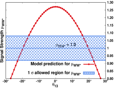
(a) The solid red curve shows the variation of $\mu_{{}_{WW^{\star}}}$ computed in our model with the CP-even mixing angle $\theta_{13}$. The shaded blue region depicts the allowed one sigma region for the measured $\mu_{{}_{WW^{\star}}}=1.00\pm 0.08$ Workman et al. (2022).

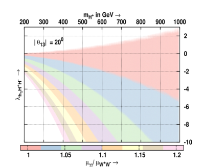
(b) Color density map for the constraint $\mu_{{}_{\gamma\gamma}}/\mu_{{}_{WW^{\star}}}$ $=1.1\pm 0.11$ Workman et al. (2022) corresponding to the $\theta_{13}=20^{\circ}$ in $(\lambda_{{h_{1}H^{+}H^{-}}}-m_{H^{\pm}}\,\,)$ plane.

Figure 1: Constraints on parameters $\theta_{13}$, $g_{{}_{h_{1}H^{+}H^{-}}}$ and $m_{H^{\pm}}\,\,$ from the measurements of the partial Higgs decay widths to the gauge bosons at the LHC Workman et al. (2022).

The partial decay width of $h_{1}\to W\,W^{\star}$ channel is related to the corresponding value in SM as

$$\Gamma(h_{1}\to WW^{\star}) = \cos^{2}\theta_{13}\ \Gamma(h^{\rm SM}\to WW^{\star})$$ (22)

giving the signal strength

$$\mu_{{}_{WW^{\star}}} = \cos^{4}\theta_{13}\ \frac{\Gamma(h^{\rm SM}\to\text{all})}{\Gamma(H\to\text{all})_{\rm LHC}}\simeq 1.27\cos^{4}\theta_{13}$$

Thus, the signal strength $\mu_{{}_{WW^{\star}}}$ depends only one parameter of the model, namely $\theta_{13}$ which can be strongly constrained by the observed value, $\mu_{WW^{\star}}=1.00\pm 0.08$ Workman et al. (2022). The one sigma band around the central value of the observed $\mu_{WW^{\star}}$ is shown in the figure 1a, which restricts the value of $\theta_{13}$ to $19.7^{\circ}\lesssim\left|\theta_{13}\right|\lesssim 22.8^{\circ}$. Throughout this work, we take $\theta_{13}=20^{\circ}$.

We now calculate the partial decay width of $h_{1}\to\gamma\gamma$ channel at one loop in our model that may be parameterized as

$$\Gamma(h_{1}\to\gamma\,\gamma) = \cos^{2}\theta_{13}\left|1+\zeta_{\gamma\gamma}\right|^{2}\,\Gamma\left(h^{\rm SM}\to\gamma\,\gamma\right),$$ (24)

where the SM Higgs partial decay width in $\gamma\,\gamma$ channel and the dimensionless parameter $\zeta_{\gamma\gamma}$ are given by Bonilla et al. (2016); Bharadwaj et al. (2021)

$$\Gamma(h^{\rm SM}\to\gamma\gamma) = \frac{G_{F}\alpha^{2}\ m_{h}^{3}}{128\sqrt{2}\pi^{3}}\ \left|\frac{4}{3}{\cal M}^{\gamma\gamma}_{1/2}\bigg{(}\frac{4m_{t}^{2}}{m_{h}^{2}}\bigg{)}+{\cal M}^{\gamma\gamma}_{1}\bigg{(}\frac{4m_{\rm W}^{2}}{m_{h}^{2}}\bigg{)}\right|^{2}$$ (25a)

$$\zeta_{\gamma\gamma} = \frac{v_{\rm SM}}{\cos\theta_{13}}\left[\frac{\frac{g_{h_{1}H^{+}H^{-}}}{2\,m^{2}_{H^{\pm}}}{\cal M}^{\gamma\gamma}_{0}\left(\frac{4m_{H^{\pm}}^{2}}{m_{h_{1}}^{2}}\right)}{{\cal M}^{\gamma\gamma}_{1}\left(\frac{4\,m_{\rm W}^{2}}{m_{h_{1}}^{2}}\right)+\frac{4}{3}\,{\cal M}^{\gamma\gamma}_{1/2}\left(\frac{4\,m_{t}^{2}}{m_{h_{1}}^{2}}\right)}\right]$$ (25b)

The loop form factors $${\cal M}^{\gamma\gamma}_{0,\,1/2,\,1}$$ in the above equations are defined in the appendix A.

Using the relations (22) and (24), the ratio of signal strengths becomes

$$\frac{\mu_{{}_{\gamma\gamma}}}{\mu_{{}_{W\,W^{\star}}}} = \frac{\Gamma(h_{1}\to\gamma\,\gamma)}{\Gamma(h_{1}\to W\,W^{\star})}\times\frac{\Gamma(h^{\rm SM}\to WW^{\star})}{\Gamma(h^{\rm SM}\to\gamma\,\gamma)}\,=\,\left|1+\zeta_{\gamma\gamma}\right|^{2}$$ (26a)

The average experimental values of signal strengths $\mu_{{}_{\gamma\gamma}}=1.10\pm{+0.07}$ and $\mu_{{}_{WW^{\star}}}=1.00\pm 0.08$ Workman et al. (2022) give $\mu_{{}_{\gamma\gamma}}/\mu_{{}_{WW^{\star}}}=1.1\pm 0.11$. The value for this ratio in our model depends only upon the parameters $\theta_{13}$, $m_{H^{\pm}}\,\,$ and $\lambda_{{h_{1}H^{+}H^{-}}}$. In the figure 1b, we depict the contours satisfying $\mu_{{}_{\gamma\gamma}}/\mu_{{}_{WW^{\star}}}=1.1\pm 0.11$ Workman et al. (2022) for $\theta_{13}=20^{\circ}$ in the ($\lambda_{{h_{1}H^{+}H^{-}}}-m_{H^{\pm}}\,\,$) plane for both positive and negative values of the triple coupling $\lambda_{{h_{1}H^{+}H^{-}}}$. It may be noted from the figure 1b that, the range of coupling $\lambda_{{h_{1}H^{+}H^{-}}}$ is bounded from below and above for a given value of $m_{H^{\pm}}\,\,$.

Since the experimental uncertainty for $\mu_{{}_{Z\gamma}}$ Workman et al. (2022) is large, we do not expect any more constraints on the the model parameters from $h_{1}\to Z\,\gamma$ decay channel Bharadwaj et al. (2021).

III.3 Constraints from LEP II Data

The scalar and pseudoscalar masses along with the Yukawa coupling $y_{1}$ in our model can be constrained from the existing LEP II data either by investigating the (a) direct pair production of scalars and pseudoscalars or (b) by production of pair of fermions mediated by these additional physical scalars or pseudoscalars. The dominant direct pair production channels at $e^{+}e^{-}$ collider:

$$e^{+}\ e^{-} \to \gamma^{\star}/\,Z^{\star}\to H^{+}+H^{-}$$ (27)

$${\rm and}\hskip 14.22636pte^{+}\ e^{-} \to Z^{\star}\to A^{0}/P^{0}+h_{i}$$ (28)

have been studied to put the lower mass bounds on $m_{H^{\pm}}\gtrsim 93.5\,$GeV and $\sum m_{h_{i}}\gtrsim 200$ GeV Schael et al. (2013). The production cross section of fermion pairs gets a contribution from additional scalars and pseudo-scalars in the model through new leptonic Yukawa coupling $y_{1}$. This additional contribution should be in agreement with the electroweak precision measurements conducted by LEP experiments. The combined analysis of DELPHI and L3 at LEP II at $\sqrt{s}=200\ GeV$ estimate the cross-section of muon pair production to Schael et al. (2013)

$$\sigma(e^{+}\ e^{-}\to\mu^{+}\ \mu^{-})=3.072\pm 0.108\pm 0.018\,{\rm pb}.$$ (29)

The excess contribution to this cross section in our model over the SM one can be written as

$$\sigma_{\mu^{+}\mu^{-}}^{\rm NP} = \frac{s}{64\pi}\ \sqrt{\frac{s-4m_{\mu}^{2}}{s-4m_{e}^{2}}}\,\left|{\cal M}_{\mu^{+}\mu^{-}}^{\rm NP}\right|^{2}$$

where

$$\left|{\cal M}_{\mu^{+}\mu^{-}}^{\rm NP}\right|^{2} = \left[y_{1}^{2}\left(-\frac{\cos^{2}\theta_{23}}{s-m_{A^{0}}^{2}}-\frac{\sin^{2}\theta_{23}}{s-m_{P^{0}}^{2}}+\frac{1}{s-m_{h_{2}}^{2}}\right)+\frac{2m_{e}m_{\mu}}{v_{{}_{\!\rm SM}}^{2}}\,\left(\frac{\cos^{2}\theta_{13}}{s-m_{h_{1}}^{2}}+\frac{\sin^{2}\theta_{13}}{s-m_{h_{3}}^{2}}\right)\right]^{2}$$ (30)

$$-\left[\frac{2m_{e}m_{\mu}}{v_{{}_{\!\rm SM}}^{2}}\,\left(\frac{1}{s-m_{h_{{}_{SM}}}^{2}}\right)\right]^{2}$$

We compute this contribution to $\mu$-pair production cross-section given by equation (30) and put constraints on the model parameters by accommodating this excess contribution within the 1$\sigma$ uncertainty (0.1095pb) in the cross-section $\sigma(e^{+}\ e^{-}\to\mu^{+}\ \mu^{-})$ given by (29). The figure 2 depicts the density maps for $\left|y_{1}\right|$ in the ($m_{{}_{h_{2}}}-\theta_{23}$) plane corresponding to various values of $m_{{}_{A^{0}}}$ and pseudo scalar mass ratio $R_{P}=m_{{}_{P^{0}}}/m_{{}_{A^{0}}}=0.5,\,1,\,2$. The value of $m_{{}_{h_{3}}}$ is taken to be 400 GeV in these plots. For a given $m_{{}_{A^{0}}}$ and $m_{{}_{P^{0}}}$, the value of $m_{h_{2}}$ has a lower limit determined by (18).

Following observations may be noted from the equation (30):

1. The cross-section is found to be less sensitive to the variation of $m_{h_{3}}$ since, for $\theta_{13}\approx 20^{\circ}$, the term proportional to $\left(m_{e}m_{\mu}\right)/v_{{}_{\!\rm SM}}^{2}$ is negligibly tiny. This enables the LEP data to tightly constrain the magnitude of the $\left|y_{1}\right|$ and $\left|\theta_{23}\right|$ for the varying scalar and pseudo-scalar masses upto a TeV scale.

2. The permitted  range  of $\left|y_{1}\right|$  is primarily governed by the choice of $\theta_{23}$ and  the pseudoscalar mass ratio  $R_{P}=m_{{}_{P^{0}}}/m_{{}_{A^{0}}}$. With the exception of $R_{P}=1$, we note that the allowed values of $\left|y_{1}\right|$ are not very sensitive to  $m_{h_{2}}$. This is because, the matrix element squared $\left|~{\cal M}_{\mu^{+}\mu^{-}}^{\rm NP}\right|^{2}$ in equation (30) becomes independent of $\theta_{23}$ for $m_{A^{0}}=m_{P^{0}}$, and hence  the allowed values of $\left|y_{1}\right|$ are dictated by vlaues of $m_{h_{2}}$ and $m_{{}_{A^{0}}}$. This is evident from the $\left|y_{1}\right|$ color density map given in figure 2b.

3. The color density maps in Figures 2a and 2c show the concave and convex profiles of $\left|y_{1}\right|$  w.r.t. $\theta_{23}$ for $R_{P}<1$ and $R_{P}>1$, respectively, due to the presence of $\cos^{2}(\theta_{23})$ and $\sin^{2}(\theta_{23})$ with the respective propagators for pseudoscalars $A^{0}$ and $P^{0}$. The convexity/ concavity profile is more pronounced for lower scalar and pseudoscalar masses.

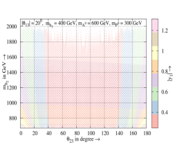
(a) $\!\!m_{{}_{A^{0}}}\!\!\!=\!600$GeV, $R_{P}\!=\!0.5$

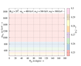
(b) $\!\!m_{{}_{A^{0}}}\!\!\!=\!300$GeV, $R_{P}\!=\!1$

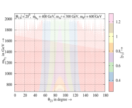
(c) $\!\!m_{{}_{A^{0}}}\!\!\!=\!300$GeV, $R_{P}\!=\!2$

Figure 2: Yukawa coupling $\left|y_{1}\right|$ color density maps for a given $\theta_{13}=20^{\circ}$ and $m_{{}_{h_{3}}}$ = 400 GeV in the ($m_{{}_{h_{2}}}-\theta_{23}$) plane satisfying the combined analysis of DELPHI and L3 $\sigma(e^{+}\ e^{-}\to\mu^{+}\ \mu^{-})=3.072\pm 0.108\pm 0.018$ pb at $\sqrt{s}=200\ GeV$ Schael et al. (2013) corresponding to the three choices of pseudo scalar mass ratios ($R_{P}=m_{{}_{P^{0}}}/m_{{}_{A^{0}}}$) $\equiv$ 1/2, 1 and 2 in Figures 2a, 2b and 2c respectively.

Working with the constrained parameter space, obtained in this section, we now proceed to look for viable explanation for the observed discrepancies in the measurements of the anomalous magnetic dipole moment for muon and the $W$-boson mass in the next two sections.

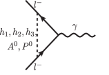
(a) Leptons 1-Loop

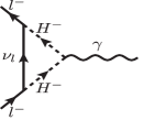
(b) Charged Scalars 1-Loop

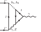
(c) BarrZee top Triangle

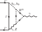
(d) BarrZee $H^{\pm}$ Triangle

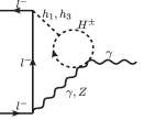
(e) BarrZee $H^{\pm}$ Bubble

Figure 3: One-loop and two-loop dominant diagrams contributing to $g-2$ of charged lepton $l$.

IV Calculation of $\mathbf{(g-2)_{\mu}}$ and $\mathbf{W}$-boson mass

We explore in this and the following sections how our model can account for the anomalies in the muon anomalous magnetic moment and the $W$-boson mass. We discuss the formalism for computing  both quantities in this section, and the following section provides the multivariate numerical analysis.

IV.1 Muon Anomalous Magnetic Moment

Now, we compute the dominant one- and two-loop contributions to the anomalous magnetic moment of a charged lepton $(l)$ in our model and then subtract the SM contributions from the same. This difference in the anomalous magnetic moment $\Delta a_{l}$ arises due to the exchange of the additional spectrum of charged and neutral scalars and pseudoscalars in the I2HDM at the one- and two-loop level of the perturbative calculations. Based on the Lagrangian given in equations (8c) and  (8i), the dominant Feynman diagrams  at one and two loops are given in the figure  3. The excess contribution to lepton $\Delta a_{l}$ at the one-loop level is given by

$$\delta a_{l}^{\rm 1\,loop} = \frac{1}{16\,\pi^{2}}\left[2\ \frac{m_{l}^{4}}{v_{{}_{\!\rm SM}}^{2}}\ \left(\frac{\cos^{2}\theta_{13}}{m_{h_{1}}^{2}}\ +\frac{\sin^{2}\theta_{13}}{m_{h_{3}}^{2}}-\frac{1}{m_{h^{\rm SM}}^{2}}\right)\ {\cal I}_{1}+m_{l}^{2}\ \left(\frac{\cos^{2}\theta_{23}}{m_{A^{0}}^{2}}+\frac{\sin^{2}\theta_{23}}{m_{P^{0}}^{2}}\right)\ y_{1}^{2}\ {\cal I}_{2}\right.$$ (31a)

$$\left.+\frac{m_{l}^{2}}{m_{h_{2}}^{2}}\ y_{1}^{2}\ {\cal I}_{1}+\left|y_{1}\right|^{2}\ \frac{m_{l}^{2}}{m_{H^{\pm}}^{2}}\ {\cal I}_{3}\right]$$

where the one loop integral functions $${\cal I}_{1},\,{\cal I}_{2} {\cal I}_{3} m_{A^{0}}=m_{P^{0}} \theta_{23}$$ and are defined in the appendix B in equations (41a),  (41b) and  (41c), respectively.  We observe that the one-loop amplitudes in Figure 3a are  negative and positive, corresponding to mediating pseudoscalars and  scalars, respectively, while  the contribution from the charged Higgs loop in Figure 3b is negative  and competitively much smaller in magnitude. It is to be noted that for , the one-loop contribution becomes independent of the mixing angle .

The contributions of two loop diagrams, some of which may dominate inspite of an additional loop suppression factor play a crucial role in the estimation of anomalous MDM. It is shown in the literature that the dominant two-loop Barr-Zee diagrams mediated by neutral scalars and pseudoscalars can become relevant for certain mass scales so that their contribution to the muon anomalous MDM are of the same order to that of one loop diagrams Chun and Mondal (2020). The additional contributions to the lepton $\Delta a_{l}$ at two-loop level is given by

$$\delta{a_{l}}^{2\ loop} = \frac{\alpha_{\rm em}}{4\ \pi^{3}}\ \left[\frac{m_{l}}{v_{{}_{\!\rm SM}}}\frac{m_{t}}{v_{{}_{\!\rm SM}}}\ \left\{\sin^{2}\theta_{13}\ f\left(\frac{m_{t}^{2}}{m_{h_{3}}^{2}}\right)-\cos^{2}\theta_{13}\ f\left(\frac{m_{t}^{2}}{m_{h_{1}}^{2}}\right)+f\left(\frac{m_{t}^{2}}{m_{h^{\rm SM}}^{2}}\right)\right\}\right.$$

$$\left.-\frac{m_{l}^{2}}{4}\,\frac{m_{l}}{v_{{}_{\!\rm SM}}^{2}}\left\{\frac{\cos\theta_{13}}{m_{h_{1}}^{2}}\ g_{{}_{h_{1}H^{+}H^{-}}}\ \tilde{f}\left(\frac{m_{H^{\pm}}^{2}}{m_{h_{1}}^{2}}\right)-\frac{\sin\theta_{13}}{m_{h_{3}}^{2}}\ g_{{}_{h_{3}H^{+}H^{-}}}\ \tilde{f}\left(\frac{m_{H^{\pm}}^{2}}{m_{h_{3}}^{2}}\right)\right\}\right]$$

where the two loop integral functions $f$ and $\tilde{f}$ are given by the equations (42a) and (42b) respectively in appendix B.

The two-loop contributions of the charged Higgs in figure 3d and 3e are comparatively small and negative. The dominant Barr-Zee contributions are found to depend on the mixing angle $\theta_{13}$, scalar masses $m_{h_{1}}$, $m_{h_{3}}$ and the Yukawa coupling $\left|y_{1}\right|$.

On analysing the combined contribution from the one- and two-loop diagrams for the constrained parameter space obtained in the preceding section, we find that, depending on the mass range of the scalars and pseudoscalars, both the one- and two-loop Barr-Zee contributions can be significant. In fact, by demanding the total anomalous magnetic dipole moment, to agree within one sigma of the measured value  as stated in equation (7), we can further limit the parameter space.

IV.2 $W$ Mass Anomaly

In this subsection, we compute the $W$-boson mass in our extended inert  two Higgs doublet models. The mass of the $W$-boson can be predicted from muon decay in terms of three  precisely measured quantities, namely, the Fermi constant, $G_{\mu}$, the fine structure constant, $\alpha_{\rm em}$, and the mass of the $Z$-boson, $m_{{}_{Z}}$ via

$$m_{{}_{W}}^{2}\left(1-\frac{m_{{}_{W}}^{2}}{m_{{}_{Z}}^{2}}\right)=\frac{\pi\alpha_{\rm em}}{\sqrt{2}G_{\mu}\left(1-\Delta r\right)}$$ (32)

where $\Delta r$ represents the quantum corrections to the relation and is a function of the scalar and pseudoscalar masses and the gauge couplings. This relationship is usually employed for predicting the $W$-boson mass $m_{{}_{W}}$ by an iterative procedure since $\Delta r$ is itself a function of $m_{{}_{W}}$. The SM contribution to $\Delta r$ at the full two-loop level, augmented by all the known three-loop contributions and the four-loop strong corrections, has been computed Degrassi et al. (2015). The discrepancy between the measured and the SM value may be resolved via quantum corrections that modify $\Delta r$. Defining $(\Delta r)^{\prime}=\Delta r\big{|}_{\rm NP}-\Delta r\big{|}_{\rm SM}$ and using measured values of $G_{\mu}$, $\alpha_{\rm em}$ and $m_{{}_{Z}}$ as input to the $SU(2)\times U(1)$ gauge theory, the relation

$$m_{{}_{W}}^{2} = (m_{{}_{W}}^{\rm SM})^{2}\left(1+\frac{s_{w}^{2}}{c_{w}^{2}-s_{w}^{2}}(\Delta r^{\prime})\right)$$ (33)

gives the prediction of $W$-boson mass Grimus et al. (2008). Here $s_{w}=\sin{\theta_{w}}$ and $c_{w}=\cos{\theta_{w}}$, $\theta_{w}$ being the weak angle and $(\Delta r^{\prime})$ represents the measure of deviations of the quantum corrections in a new physics model from those in SM. It is possible to parameterize $(\Delta r^{\prime})$ in terms of the oblique parameters $S$, $T$ and $U$ as

$$\Delta r^{\prime} = \frac{\alpha}{s_{w}^{2}}\left(-\frac{1}{2}\Delta S+c_{w}^{2}\Delta T+\frac{c_{w}^{2}-s_{w}^{2}}{4s_{w}^{2}}\Delta U\right).$$ (34)

where $\Delta S$, $\Delta T$, and $\Delta U$ are the deviations from their corresponding SM values in the estimation of the oblique parameters in any new physics models Peskin and Takeuchi (1992); *Marciano:1990dp; *Kennedy:1990ib; *Kennedy:1991sn; *Kennedy:1991wa; *Ellis:1992zi. These deviations are caused by additional radiative corrections resulting from the additional scalars and pseudoscalars in the computation of self energy amplitudes of the SM gauge bosons. The electroweak precision measurements estimate the deviations in the precision observables as  Workman et al. (2022)

$$\Delta S=-0.02\pm 0.10,\,\,\Delta T=0.03\pm 0.12,\,\,\Delta U=0.01\pm 0.11$$ (35)

Defining $\Delta m_{{}_{W}}=m_{{}_{W}}-m_{{}_{W}}^{\rm SM}$ and approximating $\Delta m_{{}_{W}}^{2}\simeq 2\,m_{{}_{W}}^{\rm SM}\Delta m_{{}_{W}}$, the discrepancy between the SM prediction and experimental value of $W$ mass can be computed using the relation

$$\Delta m_{{}_{W}}=\frac{\alpha\,m_{{}_{W}}^{\rm SM}}{2(c_{w}^{2}-s_{w}^{2})}\left(-\frac{1}{2}\Delta S+c_{w}^{2}\Delta T+\frac{c_{w}^{2}-s_{w}^{2}}{4s_{w}^{2}}\Delta U\right).$$ (36)

Since, the contribution from $\Delta U$ is small, henceforth we consider only the corrections from $\Delta S$ and $\Delta T$ to $\Delta m_{{}_{W}}$.

We compute the deviations $\Delta S$ and $\Delta T$ in our model at one loop level coming from scalars and pseudo scalars $h_{i},\,P^{0},\,A^{0}$. The explicit expressions for the same are given in the appendix C. The equation (36) can then be solved iteratively to determine the prediction of $m_{{}_{W}}$in our model.

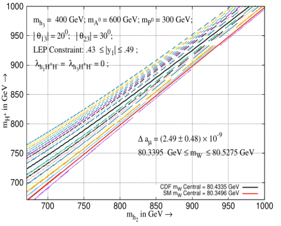
(a) $\theta_{23}=30^{\circ}$, $R_{P}=\frac{m_{{}_{P^{0}}}}{m_{{}_{A^{0}}}}=0.5$

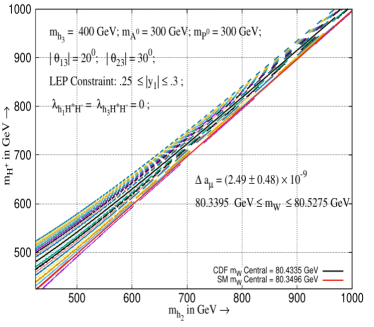
(b) $\theta_{23}=30^{\circ}$, $R_{P}=\frac{m_{{}_{P^{0}}}}{m_{{}_{A^{0}}}}=1$

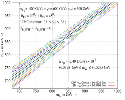
(c) $\theta_{23}=45^{\circ}$, $R_{P}=\frac{m_{{}_{P^{0}}}}{m_{{}_{A^{0}}}}=0.5$

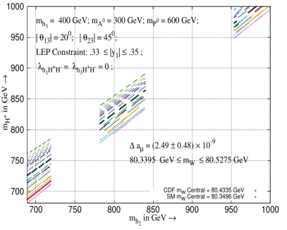
(d) $\theta_{23}=45^{\circ}$, $R_{P}=\frac{m_{{}_{P^{0}}}}{m_{{}_{A^{0}}}}=2$

Figure 4: This figure exhibits the allowed parameter space in the ($m_{{}_{h_{2}}}-m_{H^{\pm}}$) plane for various combinations of $\theta_{23}$ and $R_{P}$. In each panel, the loci of points in a given color depict a contour satisfying simultaneously  (a) LEP and partial Higgs decay width constraints from LHC, (b) a specific value of $m_{{}_{W}}=m_{{}_{W}}^{\rm CDF}+n\sigma^{\rm CDF}$, with $n\in[-10,10]$, and (c) muon anomalous  magnetic moment in the range  $[2.01\,:~\,2.97]\times 10^{-9}~$  (1$\sigma$ band of $\Delta a_{\mu}$). The lowest (uppermost) contour   corresponds to $n=-10$ ($n=10$). The loci of red and black points correspond to the central values of $m_{{}_{W}}^{\rm SM}$ and $m_{{}_{W}}^{\rm CDF}$, respectively.

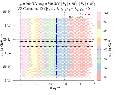
(a) $\theta_{23}=30^{\circ}$, $R_{P}=0.5$, $m_{{}_{A^{0}}}=600\,$GeV

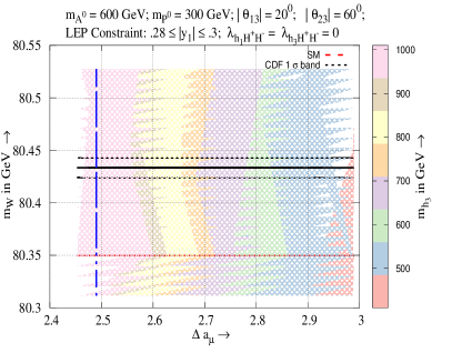
(b) $\theta_{23}=60^{\circ}$, $R_{P}=0.5$, $m_{{}_{A^{0}}}=600\,$GeV

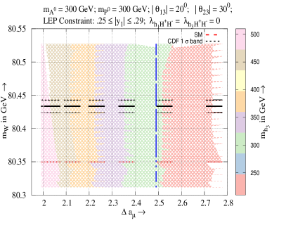
(c) $\theta_{23}=30^{\circ}$, $R_{P}=1$, $m_{{}_{A^{0}}}=300\,$GeV

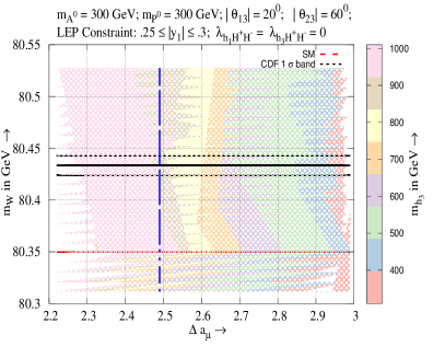
(d) $\theta_{23}=60^{\circ}$, $R_{P}=1$, $m_{{}_{A^{0}}}=300\,$GeV

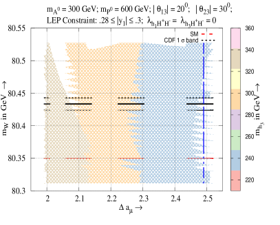
(e) $\theta_{23}=30^{\circ}$, $R_{P}=2$, $m_{{}_{A^{0}}}=300\,$GeV

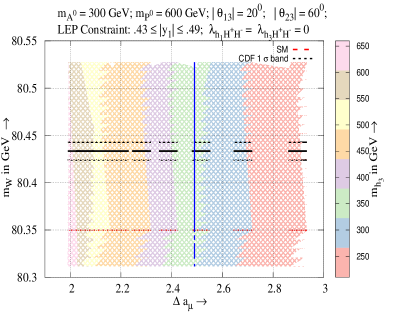
(f) $\theta_{23}=60^{\circ}$, $R_{P}=2$, $m_{{}_{A^{0}}}=300\,$GeV

Figure 5: Model prediction for twin anomalies through the $m_{h_{3}}$ color density maps in the ($\Delta a_{\mu}-m_{{}_{W}}$) plane corresponding to $\theta_{23}\equiv$ 30^∘ and 60^∘ and three choices of $R_{P}\equiv$ 0.5, 1 and 2. The density plot satisfy LEP limits and partial Higgs decay width constraint from LHC. The black horizontal dashed lines correspond to $m_{{}_{W}}^{\rm CDF}$1$\sigma$ band given by (1) while the red horizontal dashed line corresponds to $m_{{}_{W}}^{\rm SM}$predicted value (3). The vertical blue line corresponds to the central value of $\Delta a_{\mu}$ given by (7). The values of $\Delta a_{\mu}$ are shown only in the 1$\sigma$ band, i.e. in the range $[2.01:2.97]\times 10^{9}$.

V The Twin Anomaly

In this section we demonstrate the simultaneous explanation of the twin anomalies while satisfying all the constraints discussed so far. Our numerical analysis algorithm is designed as follows:

• Based on the LHC constraint on the partial decay width of Higgs to $W\,W^{\star}$ and identifying the lightest scalar in the spectrum to be $m_{h_{1}}$ = 125 GeV, we fix the CP-even mixing angle $\left|\theta_{13}\right|=20^{\circ}$.

• As discussed in section III, we divide the parameter space into three regions of pseudoscalar mass ratios: $R_{P}=m_{P^{0}}/m_{A^{0}}\equiv$ 0.5, 1, and 2. Each such region is further investigated for three choices of CP-Odd mixing angle $\theta_{23}\equiv$ $30^{\circ}$, $45^{\circ}$, and $60^{\circ}$.

• In general all scalar and pseudoscalar masses are varied between 200 GeV and 1 TeV. However, in accordance with equations (LABEL:eq:mh2a) and (LABEL:eq:mh2a), $m_{h_{2}}$ and $m_{H^{+}}$ are varied in range $\sqrt{m_{A^{0}}^{2}+m_{P^{0}}^{2}}<m_{{}_{h_{2}}},m_{{H^{\pm}}}\leq$ 1 TeV. For the purpose of demonstration and paucity of space, we choose specific mass combinations for ($m_{A^{0}},\,m_{P^{0}}$): ($600,\,300$) GeV, ($300,\,300$) GeV, and ($300,\,600$) GeV corresponding to $R_{P}=m_{P^{0}}/m_{A^{0}}\equiv$ 0.5, 1, and 2 respectively.

• The magnitude of the Yukawa coupling is kept below the perturbative limit, $\left|y_{1}\right|\leq\sqrt{4\,\pi}$. To further simplify our computation, we have considered vanishing triple scalar coupling $\lambda_{h_{i}H^{+}H^{-}}$.

• Next, we scan the constrained parameter hyperspace to search for simultaneous solution for $W$ mass lying in the range $[80.3395:80.5275]\,$ and the anomalous magnetic moment of muon lying within one sigma band $\Delta a_{\mu}\in[2.01:~2.97]\times 10^{-9}$ Aguillard et al. (2023) given in equation (7). The specified range of  $m_{{}_{W}}$ is chosen in order to include $m_{{}_{W}}^{\rm CDF}$ Aaltonen et al. (2022), $m_{{}_{W}}^{\rm PDG}$ Workman et al. (2022) and  $m_{{}_{W}}^{\rm SM}$ de Blas et al. (2022).

Following the analysis, figure 4 illustrates this allowed parameter space on the ($m_{{}_{h_{2}}}-m_{H^{\pm}}$) plane for various combinations of $\theta_{23}$ and $R_{P}$ that satisfy the one sigma permissible range for $\Delta a_{\mu}$. The lower limits of $m_{{}_{h_{2}}}$ and $m_{{}_{H^{\pm}}}$ in these plots are set by the constraint (18). The contour satisfying a specific value of $m_{{}_{W}}=m_{{}_{W}}^{\rm CDF}+n\sigma^{\rm CDF}$, with $n\in[10,10]$, is represented by the loci of points in a given color. The lowest (uppermost) contour   corresponds to $n=-10$ ($n=10$). The loci of red and black points correspond to the central values of $m_{{}_{W}}^{\rm SM}$ and $m_{{}_{W}}^{\rm CDF}$ respectively.  The choice of $\left|y_{1}\right|$ for a given set of scalar and pseudoscalar masses are essentially dictated by the LEP constraint and hence varies within a narrow range as mentioned in the legend. We make some important observations on the contour plots based on the model analysis

• Since the Yukawa coupling of leptons with $A^{0}$ and $P^{0}$ is proportional to $\cos{\theta_{23}}$ and $\sin{\theta_{23}}$ respectively, the behaviour of the contour plots for $\theta_{23}=30^{\circ}$ and $R_{P}=0.5$ is very similar to the case with $\theta_{23}=60^{\circ}$ and $R_{P}=2$. Hence we show plot for only one of them in the figure 4a.

  On the similar note, for cases where the mass ratio $R_{P}$ is unity,   the LEP constraints and the  value of $\Delta a_{\mu}$ become independent of the mixing angle $\theta_{23}$, and hence, similar patterns are obtained in the contour plots for all $\theta_{23}$. We have therefore  depicted only one of them for $\theta_{23}=30^{\circ}$ in the  figure 4b.

• No viable solution for $m_{{}_{W}}$in the required range is found for $R_{P}=2(0.5)$, at fixed $m_{h_{3}}$ = 400 GeV keeping all other parameters constant, for $\theta_{23}=30^{\circ}$($60^{\circ}$). However, given a lower (or higher) value of $m_{h_{3}}$, the solution does exists. This is also evident from the $m_{h_{3}}$ color density plot in figures 5b(5e).

• The long discontinuities of loci of points in the contour plots of figure 4 indicate the noncompliance of the model parameters to satisfy both the anomalies simultaneously in the required range.

Finally, we exhibit the sensitivity of model parameter space through the $m_{h_{3}}$ color density maps in the ($\Delta a_{\mu}-m_{{}_{W}}$) plane in figure 5 for different combinations of $R_{P}$ and $\theta_{23}$. The black horizontal lines corresponds to 1$\sigma$ band of $m_{{}_{W}}^{\rm CDF}$given by (1) while the red horizontal line corresponds to the central $m_{{}_{W}}^{\rm SM}$value (3). Similarly, the vertical blue line corresponds to the central value of $\Delta a_{\mu}$ given by (7). A couple of observations from the figure 5 are given below:

• For a given $R_{P}$, lower values of $m_{{}_{h_{3}}}$ are favored for lower values of mixing angle $\theta_{23}$. Similarly, for a given value of $\theta_{23}$, lower values of $m_{{}_{h_{3}}}$ are favored for higher $R_{P}$.

• For $\theta_{23}=30^{\circ}$ and $R_{P}=2,m_{A^{0}}=300\,$GeV, the common parameter space allowed by $m_{{}_{W}}$value favors $\Delta a_{\mu}$ in the lower half of $1\sigma$ band while for $\theta_{23}=60^{\circ}$ and $R_{P}=0.5,m_{A^{0}}=600\,$GeV, the parameter space allowed by $m_{{}_{W}}$value favors $\Delta a_{\mu}$ in the upper half of $1\sigma$ band. This can be inferred from figures 5b and 5e.

Thus, we see that a fairly large parameter space is available that solves not only the anomaly of $\Delta a_{\mu}$ but also accommodates the CDF value of $W$-boson mass. Furthermore, the model predicts the SM value of $m_{{}_{W}}$ for some parameter space that accommodates the $\Delta a_{\mu}$ observed value.

VI Summary

In this article, we have considered a minimal extension of the inert 2HDM with the inclusion of a $Z_{2}$ odd $SU(2)$ complex scalar singlet to explain the deviations of the recent measurements of the muon anomalous magnetic moment and the $W$-boson mass from their SM predictions. Implementing the stability and minimization conditions on the scalar potential, we have parameterized the model in terms of three neutral CP-even and two CP-odd scalar masses, one charged Higgs mass, one mixing angle each for the CP-even and CP-odd pair of scalars, Yukawa coupling and scalar triple couplings of charged scalar.

We identify the lightest scalar $h_{1}$ of the spectrum of this extended model with SM-like Higgs ($m_{h_{1}}$ = 125 GeV) observed at LHC. The model is then constrained by the recent measurements of the partial decay widths of Higgs to gauge bosons at the LHC that fix the CP-even mixing angle $\theta_{13}\approx 20^{\circ}$. The average experimental values of signal strengths $\mu_{{}_{\gamma\gamma}}=1.10\pm 0.07$ and $\mu_{{}_{WW^{\star}}}=1.00\pm 0.08$ Workman et al. (2022) provide the allowed range for neutral scalar triple coupling $\lambda_{{h_{1}H^{+}H^{-}}}$ with the charged Higgs. We restrict the parameter space by choosing the triple scalar couplings: $\lambda_{{h_{1}H^{+}H^{-}}}=\lambda_{{h_{3}H^{+}H^{-}}}=0.$. Further, the existing LEP data for $\sigma(e^{+}\ e^{-}\to\mu^{+}\ \mu^{-})=3.072\pm 0.108\pm 0.018\,{\rm pb}$ Schael et al. (2013) is used to constrain the relation between the Yukawa couplings and the masses of the scalar and pseudoscalars as stated in  equation (30).

We then compute the contribution of the model to the anomalous magnetic moment of the charged lepton, $\Delta a_{\mu}$, at the one loop level arising from the Feynman diagrams due to the exchange of the neutral scalar, pseudoscalar, and charged scalars as given in (31a). The contribution of the dominant Bar-Zee diagrams at the two-loop level presented in equation (LABEL:eq:MDM-2loop) is also included in the computation of $\Delta a_{\mu}$.

Next, we calculate the contribution to the precision observables $\Delta S$ and $\Delta T$  at the one loop level from the scalars and pseudoscalars in the extended I2HDM as given in the appendix C.  This deviation of the precision variables from the SM  prediction is fed into the nonlinear relation for the $W-$boson mass in equation (36). This nonlinear equation is then solved iteratively by  varying the parameters of the model to compute the contribution to $W$-boson mass in the model.

The constrained model is systematically scanned and analysed to accommodate both experimental observations simultaneously. For simplicity and brevity, the analysis is reported for three pseudoscalar mass combinations ($m_{A^{0}},m_{P^{0}}$) $\equiv$ (300,300) GeV, (300, 600) GeV, and (600,300) GeV and three choices of the pseudoscalar mixing angle $\theta_{23}\equiv 30^{\circ},45^{\circ}$, and $60^{\circ}$.  The $m_{h_{2}}$, $m_{h_{3}}$, and $m_{H^{+}}$ are varied up to 1 TeV, while the lower limits for $m_{h_{2}}$ and $m_{H^{+}}$ are fixed by the equations (LABEL:eq:mh2a) and (11b), respectively. Maintaining the unitarity of Yukawa couplings, the coupling $|y_{1}|$ is varied in range $|y_{1}|<\sqrt{4\pi}$. The allowed values of $|y_{1}|$ are fixed from the LEP data and the one sigma range for $\Delta a_{\mu}=\left(249\pm 48~\right)\times 10^{-11}$ Aguillard et al. (2023).

Our analysis can be summarised from the four panels in figure 4, where each panel consists of 22 contour plots in the ($m_{{}_{h_{2}}}-m_{H^{\pm}}$) plane for various combinations of $\theta_{23}$ and ratio $R_{P}=m_{P^{0}}/m_{A^{0}}$. The contours correspond to $10\,\sigma$ band for $m_{{}_{W}}^{\rm CDF}$ ($m_{{}_{W}}^{\rm CDF}-10\sigma^{\rm CDF}<m_{{}_{W}}<~m_{{}_{W}}^{\rm CDF}+10\sigma^{\rm CDF}$) Aaltonen et al. (2022) (in order to include $m_{{}_{W}}^{\rm SM}$) and simultaneously satisfy the one sigma permissible range for $\Delta a_{\mu}$ at fixed $m_{h_{3}}=400\,$GeV. The observations are further reinforced  by depicting the allowed common parameter space in the color density plots for $m_{h_{3}}$ in the ($\Delta a_{\mu}-m_{{}_{W}}$) plane in figure 5  for  different combinations of $R_{P}$ and  $\theta_{23}$.

Thus, the LEP and LHC data-constrained parameter hyperspaces of the said model accommodate recent observations of both $\Delta a_{\mu}$ and $m_{{}_{W}}^{\rm CDF}$within the required experimental uncertainty bands.  We also show that a different parameter space accommodating $\Delta a_{\mu}$ also predicts the SM value of $W$ mass. Although we have worked with a restricted parameter space, the simultaneous solution space of the parameters is, however, fairly large and also spans over other choices of the mass combinations for pseudoscalars with the mixing angle $20^{\circ}\leq\left|\theta_{23}\right|\leq 80^{\circ}$.   The choice of non-zero triple scalar couplings further enhances the allowed parameter space.

Appendix A Definition of Loop Form Factors

The loop amplitudes used in equations (25a) and (25b) are expressed in terms of dimensionless parameter $\tau$, which is essentially function of the ratios of mass squared of physical scalars, pseudo-scalars, gauge bosons and fermions.

$${\cal M}^{\gamma\gamma}_{0}(\tau) = -\tau[1-\tau f(\tau)]$$ (37a)

$${\cal M}^{\gamma\gamma}_{1/2}(\tau) = 2\tau[1+(1-\tau)f(\tau)],$$ (37b)

$${\cal M}^{\gamma\gamma}_{1}(\tau) = -[2+3\tau+3\tau(2-\tau)f(\tau)]$$

where

$$f(\tau)=\left\{\begin{array}[]{cc}\arcsin^{2}\big{(}\frac{1}{\sqrt{\tau}}\big{)}&\textrm{for }\,\tau\geqslant 1,\\ -\frac{1}{4}\Big{[}\log\Big(\frac{1+\sqrt{1-\tau}}{1-\sqrt{1-\tau}}\Big{missing})-i\pi\Big{]}^{2}&\textrm{for }\,\tau<1.\\ \end{array}\right.$$ (40)

Appendix B One loop and two loop functions for MDM

The integrals required to compute the one loop contribution to the muon magnetic moment of leptons (31a) are given by

$${\cal I}_{1}(r^{2}) = \int_{0}^{1}dx\ \frac{(1+x)(1-x)^{2}}{(1-x)^{2}\ r^{2}+x}$$ (41a)

$${\cal I}_{2}(r^{2}) = \int_{0}^{1}dx\ \frac{-(1-x)^{3}}{(1-x)^{2}\ r^{2}+x},$$ (41b)

$${\cal I}_{3}(r^{2}) = \int_{0}^{1}dx\ \frac{-x(1-x)}{1-(1-x)\ r^{2}}$$ (41c)

with $r=\frac{m_{l}}{m_{s_{i}}},$ and $s_{i}=h_{1},\ h_{2},\ h_{3},\ A^{0},\ P^{0}.$

The integrals contributing to the muon magnetic moment of leptons at two loop level given in equation (LABEL:eq:MDM-2loop) are defined as

$$f(r^{2}) = \frac{r^{2}}{2}\,\int_{0}^{1}dx\ \frac{1\ -\ 2x(1-x)}{x(1-x)\ -\ r^{2}}\ \ln\left[\,\frac{x(1-x)}{r^{2}}\,\right]$$ (42a)

$$\tilde{f}(r^{2}) = \int_{0}^{1}dx\ \frac{x(1-x)}{r^{2}-\ x(1-x)}\ \ln\left[\,\frac{x(1-x)}{r^{2}}\,\right]$$ (42b)

Appendix C The Oblique Parameters

The precision observables derived from the radiative corrections of the gauge Boson propagator are essentially the two point vacuum polarization tensor functions of $\Pi_{ij}^{\mu\nu}(q^{2})$, $q^{2}$ is the four-momentum of the vector boson ($V=W,Zor\gamma$). Following the prescription of the reference Haber (1993) the vacuum polarization tensor functions corresponding to pair of gauge Bosons $V_{i},V_{j}$ can be written as

$$i\Pi^{\mu\nu}_{ij}(q) = ig^{\mu\nu}A_{ij}(q^{2})+iq^{\mu}q^{\nu}B_{ij}(q^{2})\quad;\quad\quad A_{ij}(q^{2})=A_{ij}(0)+q^{2}F_{ij}(q^{2})$$ (43a)

The oblique parameters are defined as:

$$S \equiv \frac{1}{g^{2}}\left(16\pi\cos\theta_{W}^{2}\right)\left[F_{ZZ}(m_{Z}^{2})-F_{\gamma\gamma}(m_{Z}^{2})+\left(\frac{2\sin\theta_{W}^{2}-1}{\sin\theta_{W}\cos\theta_{W}}\right)F_{Z\gamma}(m_{Z}^{2})\right]$$ (44a)

$$T \equiv \frac{1}{\alpha_{em}}\left[{A_{WW}(0)\over m_{W}^{2}}-{A_{ZZ}(0)\over m_{Z}^{2}}\right]$$ (44b)

$$U \equiv \frac{1}{g^{2}}\left(16\pi\right)\left[F_{WW}(m_{W}^{2})-F_{\gamma\gamma}(m_{W}^{2})-{\cos\theta_{W}\over\sin\theta_{W}}F_{Z\gamma}(m_{W}^{2})\right]-\,S\,.$$ (44c)

$\alpha_{em}$ being the fine structure constant. It is worthwhile to mention that although $A_{ij}(0)$ and $F_{ij}$ are divergent by themselves but the total divergence associated with each precision parameter in equations (44a), (44b) and (44c) vanish on taking into account a gauge invariant set of one loop diagrams contributing for a given pair of gauge Bosons. The additional contribution to the oblique parameters (apart from SM) in our model can be computed to give

$$\Delta S = \frac{G_{F}\,\alpha_{em}^{-1}}{2\sqrt{2}\,\pi^{2}}\,\sin^{2}\left(2\,\theta_{W}\right)\,\Bigg{[}\sin^{2}\theta_{13}\bigg{\{}m_{Z}^{2}\bigg{(}\mathcal{B}_{0}(m_{Z}^{2};m_{Z}^{2},m_{h_{1}}^{2})-\mathcal{B}_{0}(m_{Z}^{2};m_{Z}^{2},m_{h_{3}}^{2})\bigg{)}+\mathcal{B}_{22}(m_{Z}^{2};m_{Z}^{2},m_{h_{3}}^{2})$$

$$-\mathcal{B}_{22}(m_{Z}^{2};m_{Z}^{2},m_{h_{1}}^{2})\bigg{\}}+\cos^{2}\theta_{23}\mathcal{B}_{22}(m_{Z}^{2};m_{h_{2}}^{2},m_{A^{0}}^{2})+\sin^{2}\theta_{23}\mathcal{B}_{22}(m_{Z}^{2};m_{h_{2}}^{2},m_{P^{0}}^{2})-\mathcal{B}_{22}(m_{Z}^{2};m_{H^{\pm}}^{2},m_{H^{\pm}}^{2})\Bigg{]}$$

where

$$\mathcal{B}_{22}(q^{2};m_{1}^{2},m_{2}^{2}) = B_{22}(q^{2};m_{1}^{2},m_{2}^{2})-B_{22}(0;m_{1}^{2},m_{2}^{2})$$ (45b)

$$\mathcal{B}_{0}(q^{2};m_{1}^{2},m_{2}^{2}) = B_{0}(q^{2};m_{1}^{2},m_{2}^{2})-B_{0}(0;m_{1}^{2},m_{2}^{2})$$ (45c)

$$\Delta T = \frac{G_{F}\,\alpha_{em}^{-1}}{2\sqrt{2}\,\pi^{2}}\Bigg{[}\sin^{2}\theta_{13}\Bigg{\{}m_{W}^{2}\bigg{(}B_{0}(0;m_{W}^{2},m_{h_{1}}^{2})-B_{0}(0;m_{W}^{2},m_{h_{3}}^{2})\bigg{)}-m_{Z}^{2}\bigg{(}B_{0}(0;m_{Z}^{2},m_{h_{1}}^{2})-B_{0}(0;m_{Z}^{2},m_{h_{3}}^{2})\bigg{)}$$ (46)

$$+B_{22}(0;m_{W}^{2},m_{h_{3}}^{2})-B_{22}(0;m_{W}^{2},m_{h_{1}}^{2})+B_{22}(0;m_{Z}^{2},m_{h_{1}}^{2})-B_{22}(0;m_{Z}^{2},m_{h_{3}}^{2})\Bigg{\}}$$

$$-\frac{1}{2}\,A_{0}(m^{2}_{H^{\pm}})+B_{22}(0;m_{H^{\pm}}\,\,^{2},m_{h_{2}}^{2})+\cos^{2}\theta_{23}\bigg{(}B_{22}(0;m_{H^{\pm}}\,\,^{2},m_{A^{0}}^{2})-B_{22}(0;m_{h_{2}}^{2},m_{A^{0}}^{2})\bigg{)}$$

$$+\sin^{2}\theta_{23}\bigg{(}B_{22}(0;m_{H^{\pm}}\,\,^{2},m_{P^{0}}^{2})-B_{22}(0;m_{h_{2}}^{2},m_{P^{0}}^{2})\bigg{)}\Bigg{]}$$

The Veltman Passarino Loop Integrals $A_{0},\,B_{0},\,B_{22}$ in the above expressions are defined as

$$A_{0}(m^{2}) = m^{2}\ \left(\Delta+1-\ln m^{2}\right),$$ (47a)

$$B_{0}(q^{2};m_{1}^{2},m_{2}^{2}) = \Delta-\int_{0}^{1}\,dx\,\ln(X-i\epsilon)$$ (47b)

$$B_{22}(q^{2};m_{1}^{2},m_{2}^{2}) = \frac{1}{4}(\Delta+1)\left[m_{1}^{2}+m_{2}^{2}-\frac{1}{3}q^{2}\right]-\frac{1}{2}\int_{0}^{1}\,dx\,X\ln(X-i\epsilon)$$ (47c)

where $X\equiv m_{1}^{2}x+m_{2}^{2}(1-x)-q^{2}x(1-x)$ and $\Delta\equiv{2\over 4-d}+\ln(4\pi)+\gamma_{E}$ in $d$ space-time dimensions. For the Feynman rules and Feynman diagrams involved in the computation of vacuum polarisation functions for $\Delta S$ and $\Delta T$, one is referred to the reference Bharadwaj et al. (2021).

References

- Crivellin and Mellado (2023) A. Crivellin and B. Mellado 10.1038/s42254-024-00703-6 (2023), arXiv:2309.03870 [hep-ph] .
- Kotwal (2024) A. V. Kotwal, Nature Rev. Phys. 6, 180 (2024).
- Aaltonen et al. (2022) T. Aaltonen et al. (CDF), Science 376, 170 (2022).
- Workman et al. (2022) R. L. Workman et al. (Particle Data Group), PTEP 2022, 083C01 (2022).
- Aad et al. (2024) G. Aad et al. (ATLAS), (2024), arXiv:2403.15085 [hep-ex] .
- de Blas et al. (2022) J. de Blas, M. Pierini, L. Reina, and L. Silvestrini, Phys. Rev. Lett. 129, 271801 (2022), arXiv:2204.04204 [hep-ph] .
- Aguillard et al. (2023) D. P. Aguillard et al. (Muon g-2), Phys. Rev. Lett. 131, 161802 (2023), arXiv:2308.06230 [hep-ex] .
- et al. (2020) T. A. et al., Physics Reports 887, 1 (2020), the anomalous magnetic moment of the muon in the Standard Model.
- Keshavarzi et al. (2020) A. Keshavarzi, D. Nomura, and T. Teubner, Phys. Rev. D 101, 014029 (2020), arXiv:1911.00367 [hep-ph] .
- Ignatov et al. (2023) F. V. Ignatov et al. (CMD-3), (2023), arXiv:2302.08834 [hep-ex] .
- Blum et al. (2023) T. Blum et al. (RBC, UKQCD), Phys. Rev. D 108, 054507 (2023), arXiv:2301.08696 [hep-lat] .
- Cici and Dag (2024) A. Cici and H. Dag, (2024), arXiv:2403.10888 [hep-ph] .
- Zhu (2023) S.-h. Zhu, AAPPS Bull. 33, 18 (2023), arXiv:2309.08633 [hep-ph] .
- (14) H. Davoudiasl, K. Enomoto, H.-S. Lee, J. Lee, and W. J. Marciano, Phys. Rev. D 108, 10.1103/PhysRevD.108.115018, arXiv:2309.04060 [hep-ph] .
- Abdallah et al. (2024) W. Abdallah, M. Ashry, J. Kawamura, and A. Moursy, Phys. Rev. D 109, 015031 (2024), arXiv:2308.05691 [hep-ph] .
- Ahmadvand and Hajkarim (2023) M. Ahmadvand and F. Hajkarim, Eur. Phys. J. C 83, 1021 (2023), arXiv:2302.09610 [hep-ph] .
- Chakrabarty et al. (2023) N. Chakrabarty, I. Chakraborty, D. K. Ghosh, and G. Saha, Eur. Phys. J. C 83, 870 (2023), arXiv:2212.14458 [hep-ph] .
- Abdallah et al. (2023) W. Abdallah, R. Gandhi, and S. Roy, Phys. Lett. B 840, 137841 (2023), arXiv:2208.02264 [hep-ph] .
- Kim et al. (2023) S.-S. Kim, H. M. Lee, A. G. Menkara, and K. Yamashita, SciPost Phys. Proc. 12, 045 (2023), arXiv:2208.12430 [hep-ph] .
- Zheng et al. (2022) M.-D. Zheng, F.-Z. Chen, and H.-H. Zhang, Eur. Phys. J. C 82, 895 (2022), arXiv:2207.07636 [hep-ph] .
- Chakrabarty (2023) N. Chakrabarty, Phys. Rev. D 108, 075024 (2023), arXiv:2206.11771 [hep-ph] .
- Kawamura and Raby (2022) J. Kawamura and S. Raby, Phys. Rev. D 106, 035009 (2022), arXiv:2205.10480 [hep-ph] .
- Chowdhury and Saad (2022) T. A. Chowdhury and S. Saad, Phys. Rev. D 106, 055017 (2022), arXiv:2205.03917 [hep-ph] .
- He (2023) S.-P. He, Chin. Phys. C 47, 043102 (2023), arXiv:2205.02088 [hep-ph] .
- Kim (2022) J. Kim, Phys. Lett. B 832, 137220 (2022), arXiv:2205.01437 [hep-ph] .
- Botella et al. (2022) F. J. Botella, F. Cornet-Gomez, C. Miró, and M. Nebot, Eur. Phys. J. C 82, 915 (2022), arXiv:2205.01115 [hep-ph] .
- Bhaskar et al. (2022) A. Bhaskar, A. A. Madathil, T. Mandal, and S. Mitra, Phys. Rev. D 106, 115009 (2022), arXiv:2204.09031 [hep-ph] .
- Arcadi and Djouadi (2022) G. Arcadi and A. Djouadi, Phys. Rev. D 106, 095008 (2022), arXiv:2204.08406 [hep-ph] .
- Kawamura et al. (2022) J. Kawamura, S. Okawa, and Y. Omura, Phys. Rev. D 106, 015005 (2022), arXiv:2204.07022 [hep-ph] .
- Zhou et al. (2022) Q. Zhou, X.-F. Han, and L. Wang, Eur. Phys. J. C 82, 1135 (2022), arXiv:2204.13027 [hep-ph] .
- Athron et al. (2023) P. Athron, A. Fowlie, C.-T. Lu, L. Wu, Y. Wu, and B. Zhu, Nature Commun. 14, 659 (2023), arXiv:2204.03996 [hep-ph] .
- Babu et al. (2022) K. S. Babu, S. Jana, and V. P. K., Phys. Rev. Lett. 129, 121803 (2022), arXiv:2204.05303 [hep-ph] .
- Bagnaschi et al. (2022) E. Bagnaschi, M. Chakraborti, S. Heinemeyer, I. Saha, and G. Weiglein, Eur. Phys. J. C 82, 474 (2022), arXiv:2203.15710 [hep-ph] .
- Bharadwaj et al. (2021) H. Bharadwaj, S. Dutta, and A. Goyal, JHEP 11, 056, arXiv:2109.02586 [hep-ph] .
- Denner et al. (2011) A. Denner, S. Heinemeyer, I. Puljak, D. Rebuzzi, and M. Spira, Eur. Phys. J. C 71, 1753 (2011), arXiv:1107.5909 [hep-ph] .
- Andersen et al. (2013) J. R. Andersen et al. (LHC Higgs Cross Section Working Group) 10.5170/CERN-2013-004 (2013), arXiv:1307.1347 [hep-ph] .
- Bonilla et al. (2016) C. Bonilla, D. Sokolowska, N. Darvishi, J. L. Diaz-Cruz, and M. Krawczyk, J. Phys. G 43, 065001 (2016), arXiv:1412.8730 [hep-ph] .
- Schael et al. (2013) S. Schael et al. (ALEPH, DELPHI, L3, OPAL, LEP Electroweak), Phys. Rept. 532, 119 (2013), arXiv:1302.3415 [hep-ex] .
- Chun and Mondal (2020) E. J. Chun and T. Mondal, JHEP 11, 077, arXiv:2009.08314 [hep-ph] .
- Degrassi et al. (2015) G. Degrassi, P. Gambino, and P. P. Giardino, JHEP 05, 154, arXiv:1411.7040 [hep-ph] .
- Grimus et al. (2008) W. Grimus, L. Lavoura, O. M. Ogreid, and P. Osland, Nucl. Phys. B 801, 81 (2008), arXiv:0802.4353 [hep-ph] .
- Peskin and Takeuchi (1992) M. E. Peskin and T. Takeuchi, Phys. Rev. D 46, 381 (1992).
- Marciano and Rosner (1990) W. J. Marciano and J. L. Rosner, Phys. Rev. Lett. 65, 2963 (1990), [Erratum: Phys.Rev.Lett. 68, 898 (1992)].
- Kennedy and Langacker (1990) D. C. Kennedy and P. Langacker, Phys. Rev. Lett. 65, 2967 (1990), [Erratum: Phys.Rev.Lett. 66, 395 (1991)].
- Kennedy and Langacker (1991) D. C. Kennedy and P. Langacker, Phys. Rev. D 44, 1591 (1991).
- Kennedy (1991) D. C. Kennedy, Phys. Lett. B 268, 86 (1991).
- Ellis et al. (1992) J. R. Ellis, G. L. Fogli, and E. Lisi, Phys. Lett. B 285, 238 (1992).
- Haber (1993) H. E. Haber, in Theoretical Advanced Study Institute (TASI 92): From Black Holes and Strings to Particles (1993) pp. 589–686, arXiv:hep-ph/9306207 .