Multipoles of the galaxy bispectrum on a light cone: wide-separation and relativistic corrections

Abstract

The galaxy bispectrum provides access to correlations among different scales that cannot be captured by the power spectrum alone, and with the Stage-IV galaxy surveys it enables the possibility of detecting both primordial non-Gaussianity (PNG) and general relativistic effects. Accounting for wide-separation corrections, which arise from the loss of symmetry in the correlation of widely separated points on the past light cone, is essential for their accurate modelling and detection. These corrections can be included perturbatively to the standard bispectrum and we compute them analytically for a generalised line of sight. We include the radial contribution to the wide-separations corrections for the first time. We show that the first-order corrections entering the odd multipoles with respect to the line of sight are large, up to $10\%$ of the bispectrum monopole, and need to be included when considering the leading-order relativistic effects that could be detectable with surveys like DESI and Euclid. The second-order wide-separation and relativistic contributions, including their mixing terms, have implications for analysis of PNG and we show, for the local type, they can mimic $f_{\rm NL}$ of order 10 in the squeezed limit. We present full analytic expressions for all these contributions to the local bispectrum and its multipoles with a publicly available code for their computation.

1 Introduction

Much effort has been employed in the use of summary statistics of galaxy clustering in redshift space to test the theoretical assumptions entering our cosmological models, from the initial conditions that gave origin to the large-scale structure (LSS) of the universe, up to the theory of gravity responsible for structure formation.

If the initial conditions were perfectly Gaussian and gravitational collapse was a linear process, the mean of the density field and its power spectrum would provide a full statistical description of the field. However, the nonlinear dynamics correlates different scales and higher-order moments are thus required to better characterise the statistical distribution of the observed fields. The bispectrum – the lowest higher-order statistics beyond the power spectrum – has been used to quantify departures from the Gaussian assumption in both matter [see 1, 2] and temperature fields [e.g., 3, 4]. The latter gives the tightest constraints to date on the level of non-Gaussianities in the initial conditions due to the small level of nonlinear structure formation at the redshifts of the cosmic microwave background (CMB). However, as CMB experiments push the limits of angular resolution to detect temperature fluctuations at smaller scales, the number of available modes are inevitably being exhausted. On the other hand, galaxy redshift surveys probe the 3D distribution of matter, resulting in many more modes to constrain cosmological parameters.

Over the past decades, these surveys have grown in the number density of detected objects and also in area and redshift range coverage [see, for example, Figure 1 of 5]. In particular, we are witnessing now the emergence of the so-called Stage-IV spectroscopic galaxy surveys, with Dark Energy Spectroscopic Instrument (DESI) [6] and Euclid [7] already in operation, and others such as SPHEREx [8] and Nancy Grace Roman Space Telescope (WFIRST) [9] to start in the upcoming years. They will enable the study of primordial physics [10] and tests of general relativity [11] with high accuracy due to the large sky fraction mapped by these surveys ($f_{\rm sky}\gtrsim 0.3$ [10]). In addition to these surveys, the Square Kilometre Array Observatory (SKAO) will conduct a low-redshift neutral hydrogen (HI) galaxy survey, during Phase-1 (SKAO1) [12], with spectroscopic precision by mapping the 21-cm radio emission of galaxies. Finally, the conceptual Phase-2 (SKAO2) would expand the observations to higher redshifts, and over a larger area (e.g., [13]).

In order to draw robust conclusions about the cosmological hypotheses one aims at testing, the observables obtained from these surveys need to be corrected for projection effects that emerge from the fact that observations are made on our past light cone [14]. The most prominent and well-studied effect are the standard redshift-space distortions (RSD) [15], which are manifested as anisotropies due to the projection of the peculiar velocity of galaxies projected along the line-of-sight (LOS) direction. However, other effects that appear in the observed redshift, such as gravitational redshift, Doppler corrections and other relativistic effects [16] are also relevant when we constrain cosmology with the galaxy number counts (e.g., see [17]).

Analyses involving redshift-space quantities decompose the induced LOS dependence of the statistics into multipoles with respect to its orientation to the LOS. In this so-called redshift space, the bispectrum has been shown to break degeneracies between the linear bias of the tracers $b_{1}$, the growth rate of structures $f$, the amplitude of linear perturbations $\sigma_{8}$ [18, 19], and neutrino masses [20], for example. Finally, further interest is directed towards the relativistic projection effects, whose leading-order contribution generate odd multipole moments in the galaxy bispectrum [21, 22, 23] and which can act as a direct probe of gravity on cosmological scales.

The convention for these multipoles is that they are calculated from the $n$-point function at local regions (defined by a singular LOS) where statistical homogeneity is assumed [24]. This approximation breaks down at large scales since the statistics of the density field at each point in the local correlation function is different. Corrections to this singular LOS approximation can be done through a series expansion, where it becomes dependent on the actual choice of the LOS in the triplet.

Although the angular part of these corrections, induced as we leave the local plane-parallel limit, has been extensively studied for the case of the two-point statistics [25, 26, 27, 28, 29, 30, 31, 32, 33, 34, 35], giving rise to the so-called wide-angle corrections, their impact on the galaxy bispectrum [for example, see 36] and corrections that appear by breaking statistical homogeneity radially [37, 31, 34, 35] are much less common. It was only recently that wide-angle corrections were computed for the bispectrum in a Cartesian-Fourier basis in [38]. The consistency of [38] was then verified with a different basis expansion in [39]. In these works, it is shown that wide-angle effects in the bispectrum can bias the detection of PNG of the local type, a specific signal which emerges from a quadratic correction to the primordial gravitational potential [40, 41].

Indeed, with Stage-IV surveys, these corrections become relevant not only due to the increased precision, but also as these surveys map increased volume the scales that are correlated increase. In this work, we attempt to provide a consistent picture of the relative contribution of relativistic, wide angle and radial redshift terms to the bispectrum multipoles over a range of bispectrum shapes and scales and how this depends on the LOS used to describe the local triplet.

Wide-separation terms are suppressed by a factor $(1/k\,d)^{m}$ for a given order in the perturbative expansion, while the relativistic terms have suppression factors of $(\mathcal{H}/k)^{n}$. In this work, we calculate terms up to second-order ($m+n\leq 2$), including cross-terms, and we highlight how wide-separation corrections have the potential to impact both the analysis of both the imaginary relativistic contribution and also PNG.

This paper is organised as follows. In Section 2, we introduce the local bispectrum along with the relevant perturbation theory, as well detail on the relativistic corrections. In Section 3, we present the perturbative framework to include wide-separation effects in the bispectrum. The results are presented and discussed in Section 4, and we conclude in Section 5.

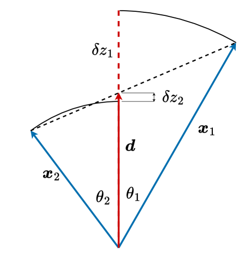
Figure 1: Real space two-point function, where deviations from the plane-parallel and constant redshift limit are respectively expressed in terms of $\theta_{1},\theta_{2}$ and $\delta z_{1},\delta z_{2}$ for a given LOS $\bm{d}$.

2 The Local Bispectrum

In the case of a statistically homogeneous field our statistics are more straightforward with fewer degrees of freedom, e.g. in the case of the power spectrum it is diagonal and the bispectrum is zero for open triangles. Indeed, without statistical homogeneity the standard approach to expand the Fourier space correlators into multipoles with respect to the orientation to the LOS becomes ill-defined [42, 43, 32] and different statistics are needed.

While we assume the density field to be statistically homogeneous in real-space for a constant time slice, in reality, when we observe on a light cone, this symmetry is broken by a couple of effects. Firstly, redshift-space distortions cause our field in redshift space to depend on the LOS; for a survey outside the plane-parallel limit, different regions within the survey will be statistically different due to the differing LOS. Secondly, on the past light cone, the statistics change radially as the density field evolves with redshift.

Therefore, it is useful and conventional to define local regions which are approximated to be statistically homogeneous [24], and as such they can be described by a singular LOS. In this case, therefore, the statistics are diagonal.

The local 3-point function is thus described by a triplet of points defined at a certain point in space, which define our local bispectrum after a Fourier transformation,

$$B^{\rm loc}(\bm{k}_{1},\bm{k}_{2},\bm{d})\equiv\int\mathrm{d}^{3}\bm{x}_{13}\mathrm{d}^{3}\bm{x}_{23}\,{\rm e}^{-i(\bm{k}_{1}\cdot\bm{x}_{13}+\bm{k}_{2}\cdot\bm{x}_{23})}\,\langle\delta(\bm{x}_{1})\delta(\bm{x}_{2})\delta(\bm{x}_{3})\rangle,$$ (2.1)

where $\bm{x}_{13}=\bm{x}_{1}-\,\bm{x}_{3}$ and the dependence on $\bm{d}$ is implicit in the 3-point correlation function given by $\langle\delta(\bm{x}_{1})\delta(\bm{x}_{2})\delta(\bm{x}_{3})\rangle\equiv\zeta(\bm{x}_{1},\bm{x}_{2},\bm{x}_{3})\equiv\zeta(\bm{x}_{13},\bm{x}_{23},\bm{d})$.

The full local bispectrum in redshift space can parameterised with six degrees of freedom: $B_{\rm loc}(q_{1},q_{2},q_{3},\mu_{1},\phi_{12};d)$, three of which, $k_{1},k_{2},k_{3}$, describe the triangle shape and two more, $\theta_{1},\phi_{12}$, describe the orientation of the triangle with respect to the LOS, and $d$ is the separation of the observer to the triplet. We define $\theta$ as the angle between $\bm{k}_{1}$ and the LOS, $\bm{d}$, such that $\cos(\theta_{1})=\mu_{1}=\bm{k}\cdot\bm{d}$ and $\phi$ are the azimuthal angles between $\bm{k}_{2}$ and $\hat{\bm{d}}$ in the plane normal to $\hat{\bm{k}}_{1}$. Therefore, they satisfy

$$\mu_{2}=\mu_{1}\cos{\theta}+\sqrt{1-\mu^{2}}\sin{\theta}\cos{\phi_{12}},$$ (2.2)

where $\cos{\theta}=\hat{\bm{k}}_{1}\cdot\hat{\bm{k}}_{2}$.

2.1 Multipoles estimator

If we construct the standard ‘Scoccimarro’ estimator for the bispectrum multipoles [24]

$$\hat{B}_{\ell m}(k_{1},k_{2},k_{3})=\frac{1}{N^{T}_{123}}\int_{\mathcal{S}_{1}} \frac{\mathrm{d}^{3}\bm{q}_{1}}{(2\pi)^{3}}\int_{\mathcal{S}_{2}}\frac{\mathrm{d}^{3}\bm{q}_{2}}{(2\pi)^{3}}\int_{\mathcal{S}_{3}}\frac{\mathrm{d}^{3}\bm{q}_{3}}{(2\pi)^{3}}\,\,\delta^{D}(\bm{q}_{123})\int\mathrm{d}^{3}\bm{x}_{1}\,\mathrm{d}^{3}\bm{x}_{2}\,\mathrm{d}^{3}\bm{x}_{3}$$ (2.3)

$$\times{\rm e}^{-i(\bm{k}_{1}\cdot\bm{x}_{13}+\bm{k}_{2}\cdot\bm{x}_{23})}\,\,\delta_{W}(\bm{x}_{1})\,\delta_{W}(\bm{x}_{2})\,\delta_{W}(\bm{x}_{3})\,Y^{*}_{\ell,m}(\hat{\bm{q}}_{1}\cdot\hat{\bm{d}},\phi),$$

where the orientation of the triangle relative to the LOS $\hat{\bm{d}}$ is decomposed into spherical harmonics about $\hat{\bm{d}}$. Note, however, the $m\neq 0$ parts are not computable with separable Fast Fourier Transforms (FFT), and so it is common to just focus on the $m=0$ part, which can be written in terms of a Legendre basis. Further, since this is measured in a survey, we define the windowed density field $\delta_{W}(\bm{x})=W(\bm{x})\delta(\bm{x})$, where $W(\bm{x})$ is the survey window function. The Fourier space integrals are discrete sums $\int_{\mathcal{S}_{i}}\mathrm{d}^{3}\bm{q}_{i}F(\bm{q}_{i})\equiv\sum_{\mathcal{S}_{i}}F(\bm{q}_{i})$ over thin $k$-space shells $\mathcal{S}_{i}$ of width $\Delta k$, centred at $k_{i}$, such that $\mathcal{S}_{i}\equiv\mathcal{S}(k_{i}|\Delta k)$ is the region of $k$-magnitudes contained by a given $k_{i}$-bin, $k_{i}-\Delta k/2\leq k\leq k_{i}+\Delta k/2$. Here, $N^{T}_{123}$ represents the number of closed triangles formed from the triplet of bins,

$$N^{T}_{123}=k_{f}^{-3}\int_{\mathcal{S}_{1}}\mathrm{d}^{3}\bm{q}_{1}\int_{\mathcal{S}_{2}}\mathrm{d}^{3}\bm{q}_{2}\int_{\mathcal{S}_{3}}\mathrm{d}^{3}\bm{q}_{3}\,\,\delta^{D}(\bm{q}_{123}),$$ (2.4)

where $k_{f}$ is the fundamental frequency in Fourier space. We can then construct the equivalent unwindowed theoretical expectation that corresponds to the ‘Scoccimarro’ estimator for each multipole $B_{\ell m}$ [24]. In the continuous limit, using the change in coordinates

$$\int\mathrm{d}^{3}\bm{x}_{1}\mathrm{d}^{3}\bm{x}_{2}\mathrm{d}^{3}\bm{x}_{3}\rightarrow\int\mathrm{d}^{3}\bm{d}\int\mathrm{d}^{3}\bm{x}_{13}\mathrm{d}^{3}\bm{x}_{23},$$ (2.5)

and splitting the integration in each shell

$$\int_{\mathcal{S}_{i}}\mathrm{d}^{3}\bm{q}_{i}=\int^{k_{i}+\Delta k/2}_{k_{i}-\Delta k/2}\mathrm{d}q_{i}q_{i}^{2}\int\mathrm{d}\Omega_{q_{i}},$$ (2.6)

where $\int\mathrm{d}\Omega_{q}$ represents an integral over solid angle, the corresponding theoretical multipoles can be expressed in the familiar form:

$$B_{\ell m}(k_{1},k_{2},k_{3})=\int\frac{\mathrm{d}^{3}\bm{d}}{V_{s}}\left[\int\frac{\mathrm{d}\Omega}{4\pi}B^{\rm loc}(q_{1},q_{2},q_{3},\mu_{1},\phi_{12};d)Y^{*}_{\ell m}(\mu_{1},\phi_{12})\right].$$ (2.7)

It is convenient to define the term in the square bracket above as the local bispectrum multipole, such that the multipoles measured with a given survey corresponds to an average of this local quantity over the entire survey volume.

Equivalently, we could consider alternative decompositions for the anisotropic local bispectrum, such as the tri-polar spherical harmonic (TripoSH) [44] or other modal approaches (e.g., see [45]), where wide-separation corrections are still computed from the local bispectrum, but they will enter a different set of multipoles and modes.

2.2 Perturbation theory

In this section we give a brief overview of the perturbation theory that forms the basis of our later calculations; the aim is to write the theoretical local bispectrum with explicit dependence on the ‘end-point’ positions, $\bm{x}_{1},\bm{x}_{2},\bm{x}_{3}$, including where we have redshift dependent functions. See [46] for a more detailed review of these topics.

The local bispectrum correlates density fields at different radial comoving distances, $x_{i}$, which corresponds to different redshifts, $z_{i}$. Therefore, we express this redshift dependence in terms of the radial comoving distances. We also adopt the following notation for real and Fourier integrals;

$$\int_{\bm{x}}\equiv\int\mathrm{d}^{3}\bm{x}\,\,,\,\,\int_{\bm{q}}\equiv\int\frac{\mathrm{d}^{3}\bm{q}}{(2\pi)^{3}}.$$ (2.8)

In standard perturbation theory we can express both the matter overdensity $\delta(\bm{x})$ and velocity divergence $\theta(\bm{x})=\nabla\cdot\bm{v}(\bm{x})$ fields neatly in Fourier space as a perturbative sum where each $n^{\rm th}$ order field can be expressed in terms of $n$ products of first order density field with some coupling kernel. For example, we can write

$$\delta(\bm{k},x) =\sum_{n=1}^{\infty}\int_{\bm{k}_{1},...,\bm{k}_{n-1},\bm{k}_{n}}\delta_{D}(\bm{k}-\bm{k}_{1}-...-\bm{k}_{n})F_{n}(\bm{k}_{1},...,\bm{k}_{n},x)\delta^{(1)}(\bm{k}_{1},x)...\delta^{(1)}(\bm{k}_{n},x),$$ (2.9a)

$$\theta(\bm{k},x) =-f\mathcal{H}\sum_{n=1}^{\infty}\int_{\bm{k}_{1},...,\bm{k}_{n-1},\bm{k}_{n}}\delta_{D}(\bm{k}-\bm{k}_{1}-...-\bm{k}_{n})G_{n}(\bm{k}_{1},...,\bm{k}_{n},x)\delta^{(1)}(\bm{k}_{1},x)...\delta^{(1)}(\bm{k}_{n},x),$$ (2.9b)

where $F_{n}(\bm{k}_{1},...,\bm{k}_{n},x_{1})$ and $G_{n}(\bm{k}_{1},...,\bm{k}_{n},x_{1})$ are the perturbation theory kernels responsible for the coupling of scales, $f$ is the linear growth rate of matter perturbations, and $\mathcal{H}$ is the conformal Hubble parameter.

At first order, the density field can be separated into its temporal and spatial parts:

$$\delta^{(1)}(\bm{k}_{1},x_{1})=D(x_{1})\delta^{(1)}(\bm{k}_{1}),$$ (2.10)

where the time evolution is parameterised by the linear growth function, $D(x_{1})$, satisfying the equation

$$\mathcal{H}^{2}(x_{1})(1+z(x_{1}))^{2}D_{zz}(x_{1})+[\mathcal{H}_{z}(x_{1})\mathcal{H}(x_{1})(1+z(x_{1}))^{2}]D_{z}=\frac{3H_{0}^{2}\Omega_{m,0}}{2a(x_{1})}D(x_{1}),$$ (2.11)

where derivatives of a function $F$ with respect to redshift are denoted by $F_{z}$.

For the case of a field at second order, this can be expressed in terms of a convolution of two first-order fields with the relevant coupling kernel (e.g., Equation 2.9). At second order, this split is not so trivial; however, it can be solved to provide a solution for the Fourier-space Newtonian coupling kernels (see, for example, [47, 48]):

$$F_{2}(\bm{q}_{1},\bm{q}_{2},x_{1}) =\frac{1}{2}[1+K(x_{1})]+\frac{1}{2}\hat{\bm{q}}_{1}\cdot\hat{\bm{q}}_{2}\left(\frac{q_{2}}{q_{1}}+\frac{q_{2}}{q_{2}}\right)+\frac{[1-K(x_{1})]}{2}(\hat{\bm{q}}_{1}\cdot\hat{\bm{q}}_{2})^{2},$$ (2.12a)

$$G_{2}(\bm{q}_{1},\bm{q}_{2},x_{1}) =C(x_{1})+\frac{1}{2}\hat{\bm{q}}_{1}\cdot\hat{\bm{q}}_{2}\left(\frac{q_{2}}{q_{1}}+\frac{q_{2}}{q_{2}}\right)+[1-C(x_{1})](\hat{\bm{q}}_{1}\cdot\hat{\bm{q}}_{2})^{2},$$ (2.12b)

where, following the same notation as [47], the redshift-dependent coefficients are defined by the relationship of the first and second-order growth functions, $D$ and $F$ respectively, such that

$$K(x_{1})\equiv\frac{F(x_{1})}{D^{2}(x_{1})},\,\,C(x_{1})\equiv\frac{F^{\prime}(x_{1})}{2D(x_{1})D^{\prime}(x_{1})}.$$ (2.13)

The second-order growth rate satisfies a differential equation similar to the one at first-order, but with an additional source term

$$\mathcal{H}^{2}(x_{1})[1+z(x_{1})]^{2}F_{zz}(x_{1})+\left(\mathcal{H}_{z}(x_{1})\,\mathcal{H}(x_{1})\,[1+z(x_{1})]^{2}\right)F_{z}(x_{1})=\frac{3H_{0}^{2}\Omega_{m,0}}{2a(x_{1})}[F(x_{1})+D^{2}(x_{1})].$$ (2.14)

In the Einstein-de-Sitter limit, we recover the standard approximation for the second order kernels, where $K(x_{1})=C(x_{1})=3/7$.

The standard first- and second-order redshift space Newtonian kernels with explicit $\bm{x}_{1},\bm{x}_{2}$ and $\bm{x}_{3}$ are given by [18, 49]

$$Z^{(1)}_{\rm N}(\bm{q},\bm{x}_{1})=D(x_{1})[b_{1}+f(\hat{\bm{q}}\cdot\hat{\bm{x}}_{1})^{2}],$$ (2.15)

and

$$Z^{(2)}_{\rm N}= D^{2}(x_{1})\left(b_{1}(x_{1})\left(F_{2}(\bm{q}_{1},\bm{q}_{2},x_{1})\right)+\frac{b_{2}(x_{1})}{2}\right.$$ (2.16)

$$\left.+\,f(x_{1})\frac{(\bm{q}_{12}\cdot\hat{\bm{x}}_{1})^{2}}{q^{2}_{12}}\left(G_{2}(\bm{q}_{1},\bm{q}_{2},x_{1})\right)+b_{\Gamma_{2}}(x_{1})S(\bm{q}_{1},\bm{q}_{2})\right.$$

$$\left.+\frac{f(x_{1})}{2}(\bm{q}_{12}\cdot\hat{\bm{x}}_{1})\left[b_{1}(x_{1})\left(\frac{(\bm{q}_{1}\cdot\hat{\bm{x}}_{1})}{q_{1}^{2}}+\frac{(\bm{q}_{2}\cdot\hat{\bm{x}}_{1})}{q_{2}^{2}}\right)+f(x_{1})\frac{(\bm{q}_{1}\cdot\hat{\bm{x}}_{1})(\bm{q}_{2}\cdot\hat{\bm{x}}_{1})}{q_{1}^{2}q^{2}_{2}}(\bm{q}_{12}\cdot\hat{\bm{x}}_{1})\right]\right)$$

where $\bm{q}_{12}=\bm{q}_{1}+\bm{q}_{2}$, $b_{1}$ and $b_{2}$ are the Eulerian linear and second order clustering biases respectively, and $b_{\Gamma_{2}}$ is the tidal bias with the kernel,

$$\mathcal{S}_{2}(\bm{q}_{1},\bm{q}_{2})=(\hat{\bm{q}}_{1}\cdot\hat{\bm{q}}_{2})^{2}-1$$ (2.17)

As wide-separation and relativistic effects are generally relevant only on large scales, we ignore higher-order loop contributions and the phenomenological Fingers-of-God (FoG) damping that affects the bispectrum on smaller, nonlinear scales. Though we note that mixing between these contributions will still be non-negligible for the bispectrum, particularly in the squeezed limit as it correlates both large and small scales, we leave this modelling to future work.

2.3 Relativistic effects

Relativistic distortions occur as we observe on our past light cone. These distortions include projection type effects arising from the Doppler-type effects and gravitational redshift as well as integrated effects like the Integrated Sachs-Wolfe (ISW) and lensing contributions.

Relativistic projection effects been well studied in linear perturbation theory [50, 14, 51]. At second order the picture is more complicated [52, 53, 54, 55, 56, 57], with extra couplings between the projection effects and additional dynamical contributions arising from relativistic treatment of the second order gravitational and velocity potentials.

Here we will make use of the calculations presented in [58, 59, 60, 61, 22], which includes all local corrections arising from projection effects along the LOS, as well as contributions from the dynamical evolution. We neglect integrated terms in common with these works, though these will be interesting to include in a more complete analysis.

Keeping terms up to $(\mathcal{H}/k)^{2}$, the relativistic part of the redshift-space kernels are given by

$$Z^{(1)}_{\rm GR}=i\, (\bm{q}_{1}\cdot\hat{\bm{x}}_{1})\frac{\gamma_{1}}{q_{1}^{2}}+\frac{\gamma_{2}}{q_{1}^{2}},$$ (2.18a)

$$\begin{split}Z^{(2)}_{\rm GR}=\frac{1}{q^{2}_{1}q^{2}_{2}}\bigg{(}&\frac{q^{2}_{1}q^{2}_{2}}{q^{2}_{3}}\left[F_{2}(\bm{q}_{1},\bm{q}_{2})\beta_{6}+G_{2}(\bm{q}_{1},\bm{q}_{2})\beta_{7}\right]+(\bm{q}_{1}\cdot\hat{\bm{x}}_{1})(\bm{q}_{2}\cdot\hat{\bm{x}}_{1})\beta_{8}\\ &+(\bm{q}_{3}\cdot\hat{\bm{x}}_{1})^{2}\left(\beta_{9}+E_{2}(\bm{q}_{1},\bm{q}_{2})\beta_{10}\right)+(\bm{q}_{1}\cdot\bm{q}_{2})\beta_{11}+(q^{2}_{1}+q_{2}^{2})\beta_{12}\\ &+((\bm{q}_{1}\cdot\hat{\bm{x}}_{1})^{2}+(\bm{q}_{2}\cdot\hat{\bm{x}}_{1})^{2})\beta_{13}\\ &+i\Big{\{}[(\bm{q}_{1}\cdot\hat{\bm{x}}_{1})q_{1}^{2}+(\bm{q}_{2}\cdot\hat{\bm{x}}_{1})q_{2}^{2}]\beta_{14}+\left[(\bm{q}_{1}\cdot\hat{\bm{x}}_{1})+(\bm{q}_{2}\cdot\hat{\bm{x}}_{1})\right](\bm{q}_{1}\cdot\bm{q}_{2})\beta_{15}\\ &\quad+q_{1}q_{2}[(\bm{q}_{1}\cdot\hat{\bm{x}}_{1})+(\bm{q}_{2}\cdot\hat{\bm{x}}_{1})]\beta_{16}+[(\bm{q}_{1}\cdot\hat{\bm{x}}_{1})^{3}+(\bm{q}_{2}\cdot\hat{\bm{x}}_{1})^{3})]\beta_{17}\\ &\quad+(\bm{q}_{1}\cdot\hat{\bm{x}}_{1})(\bm{q}_{2}\cdot\hat{\bm{x}}_{1})[(\bm{q}_{1}+\bm{q}_{2})\cdot\hat{\bm{x}}_{1}]\beta_{18}+(\bm{q}_{3}\cdot\hat{\bm{x}}_{1})\frac{q^{2}_{1}q^{2}_{2}}{q^{2}_{3}}G_{2}(\bm{q}_{1},\bm{q}_{2})\beta_{19}\Big{\}}\bigg{)},\end{split}$$ (2.18b)

where

$$E_{2}(\bm{q}_{1},\bm{q}_{2})=\frac{q^{2}_{1}q^{2}_{2}}{q^{4}_{3}}\left[3+2\hat{\bm{q}}_{1}\cdot\hat{\bm{q}}_{2}\left(\frac{q_{2}}{q_{1}}+\frac{q_{2}}{q_{2}}\right)+(\hat{\bm{q}}_{1}\cdot\hat{\bm{q}}_{2})^{2}\right].$$ (2.19)

The time dependence (e.g., dependence on radial comoving distance) is contained within the $\gamma$’s and $\beta$’s, for the first and second orders respectively, which are bias dependent coefficients evaluated at $x_{i}$. For example, $\gamma_{1}$ the leading order relativistic correction and $\gamma_{2}$ the second order part can be written as,

$$\frac{\gamma_{1}(x_{1})}{\mathcal{H}(x_{1})} =f(x_{1})\left[b_{e}(x_{1})-2\mathcal{Q}(x_{1})-\frac{2(1-\mathcal{Q}(x_{1}))}{x_{1}\,\mathcal{H}(x_{1})}-\frac{-(1+z(x_{1}))\mathcal{H}(x_{1})\mathcal{H}_{z}(x_{1})}{\mathcal{H}^{2}(x_{1})}\right],$$ (2.20a)

$$\begin{split}\frac{\gamma_{2}(x_{1})}{\mathcal{H}^{2}(x_{1})}&=f(x_{1})(3-b_{e}(x_{1}))+\frac{3}{2}\Omega_{m}(x_{1})\bigg{[}2+b_{e}(x_{1})-f(x_{1})-4\mathcal{Q}(x_{1})\\ &\hskip 155.0pt-\frac{2(1-\mathcal{Q}(x_{1}))}{x_{1}\,\mathcal{H}(x_{1})}-\frac{-(1+z(x_{1}))\mathcal{H}(x_{1})\mathcal{H}_{z}(x_{1})}{\mathcal{H}(x_{1})^{2}}\bigg{]}.\end{split}$$ (2.20b)

Here, $\mathcal{Q}$ and $b_{e}$ are respectively the magnification and evolution biases and $\Omega_{m}$ is the matter density parameter.

The leading-order relativistic terms are projection effects arising from the redshift-space projection, with the Doppler and gravitational redshift contributions. These terms, represented by $\gamma_{1}$ and $\beta_{14}-\beta_{19}$, are imaginary and scale as $\mathcal{H}/k$; they are also of odd parity and, as such, they contribute to the odd multipole moments [61, 22]. While the second-order terms that scale as $(\mathcal{H}/k)^{2}$ are real and contribute to the even multipoles. Full expressions for the $\beta$’s are given in Appendix A of [22].

2.4 Local tree-level bispectrum

The redshift-space kernels, including the relativistic parts, are given by

$$Z^{(1)} =Z^{(1)}_{\rm N}+Z^{(1)}_{\rm GR},$$ (2.21a)

$$Z^{(2)} =Z^{(2)}_{\rm N}+Z^{(2)}_{\rm GR}.$$ (2.21b)

By considering the definition of the local bispectrum (Equation (2.1)), the configuration space density fields, $\delta_{s}(\bm{x})$, can be expressed in terms of the inverse Fourier transform of the standard redshift-space fields, $\delta_{s}(\bm{k})$, such that the leading-order local bispectrum can be expressed as

$$B_{\text{loc}}(k_{1},k_{2},k_{3},\mu_{1},\phi)=\int_{\bm{x}_{13},\bm{x}_{23},\bm{q}_{1},\bm{q}_{2}} {\rm e}^{-i[(\bm{k}_{1}-\bm{q}_{1})\cdot\bm{x}_{13}+(\bm{k}_{2}-\bm{q}_{2})\cdot\bm{x}_{23}]}$$ (2.22)

$$\times 2Z^{(1)}(\bm{q}_{1},\bm{x}_{1})Z^{(1)}(\bm{q}_{2},\bm{x}_{2})Z^{(2)}(\bm{q}_{1},\bm{q}_{2},\bm{x}_{3})P(q_{1})P(q_{2}).$$

3 Wide-Separation Corrections

The local bispectrum correlates the density field in three separate locations in the sky (see Equation 2.1), which under the assumption of local homogeneity is modelled by a single LOS. As in the global case, this assumption is also broken locally due to redshift space distortions outside the plane parallel limit and due to the redshift evolution. Thus, describing the triplet by a singular LOS, $\bm{d}$, results in a loss of signal; in observations, the density fields at these positions are statistically different. To include the full non-linear wide-separation corrections, one would therefore need to compute a statistic dependent on all 3 end-point positions. However, just as in the power spectrum, these corrections can be approximated by introducing a series expansion to account for the deviations of the triplet positions from the chosen LOS, $\bm{d}$.

These corrections for the position of each point in the triplet can naturally be split into angular and radial parts. The angular components are termed ‘wide-angle’ (WA) corrections and arises as we leave the local plane-parallel limit, such that $\hat{\bm{x}}_{1}\neq\hat{\bm{x}}_{2}\neq\hat{\bm{x}}_{3}$; the magnitude of these corrections are therefore dependent on the size of the opening angle between the triplet and the observer, which can be defined in terms of $(x_{13}/d)$ and $(x_{23}/d)$. Corrections to the radial part arise as these statistics are measured on a light cone, and the points in the triplet are at differing comoving distances, such that $x_{1}\neq x_{2}\neq x_{3}$, corresponding to different redshifts. Hence, these terms depend on the size of the radial separation and on how the cosmology changes with redshift. We introduce the term ‘radial redshift’ (RR) to label these corrections.

Perturbative expansions to include wide-separation corrections are performed on the triangle in configuration space, and thus it is relatively straightforward to include them in the correlation functions; however, for Fourier-space statistics, the calculation is slightly more involved. The standard approach for the power spectrum is to perform the expansion in configuration space, computing the multipoles of the two-point correlation function first, and then Hankel transforming this to get the multipoles of the power spectrum [31, 32]. This type of approach was extended to the bispectrum in [39], where the angular dependencies of the three-point correlation function (3PCF) were expanded into Legendre multipoles and as such, after computing the angular integrals, the 3PCF can be related to the bispectrum multipoles by a double Hankel transform.

In [38], a formalism using a Cartesian space expansion is introduced. This allows for the computation of wide-separation corrections directly in Fourier space. This approach has the advantage that it connects neatly with standard perturbation theory (SPT) in Fourier space and, therefore, is easily extendable to higher-order statistics. When comes to the bispectrum, this method also has the advantage of being fully analytic and only reliant on finite sums. Here, we use this formalism to compute wide-separation corrections, including radial-redshift corrections, for a generalised LOS. Below we describe our calculations.

3.1 Geometry in configuration space

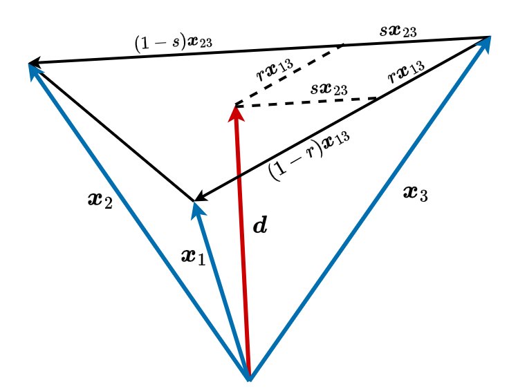
Figure 2: Bispectrum geometry in real space, where the LOS $\bm{d}$ and the positions of the real space end-points LOS defined from the observer. The parameters $r$ and $s$ are the weights relating $\bm{d}$ to $\bm{x}_{3}$.

The choice of LOS here then represents both the point from which we perform our expansions but also the unit vector which we use to define our spherical harmonics multipoles. This choice can be generalized to any point in the real-space triangle defined by $\bm{x}_{1},\bm{x}_{2},\bm{x}_{3}$ using two free parameters such that

$$\bm{d}=r\,\bm{x}_{1}+s\,\bm{x}_{2}+(1-r-s)\,\bm{x}_{3},$$ (3.1)

where $0<r+s<1$ and are defined with respect to $\bm{x}_{3}$.

From this parameterisation, the three end-point LOS $\bm{x}_{1},\bm{x}_{2}$ and $\bm{x}_{3}$ can be re-expressed in terms of the parameters of our local bispectrum, Equation (2.1): $\bm{d}$, at which we define our local bispectrum, and $\bm{x}_{13}$ and $\bm{x}_{23}$, which are integrated over. By inspecting Figure 2), we see that we can write, for example,

$$\bm{x}_{1} =\bm{d}+(1-r)\bm{x}_{13}-s\bm{x}_{23},$$ (3.2)

$$\bm{x}_{2} =\bm{d}-r\bm{x}_{13}+(1-s)\bm{x}_{23},$$

$$\bm{x}_{3} =\bm{d}-r\bm{x}_{13}-s\bm{x}_{23}.$$

Common LOS choices, such as the end-point or centre-of-mass (COM), are then defined as:

$$\bm{x}_{1} :\,\,r=1,\quad s=0,$$ (3.3)

$$\bm{x}_{2} :\,\,r=0,\quad s=1,$$

$$\bm{x}_{3} :\,\,r=0,\quad s=0,$$

COM $$:\,\,r=s=1/3.$$

For convenience in the series expansion below, we also define the notation

$$A_{i} =\begin{cases}A_{1}=(1-r),&\text{for }\bm{x}_{1}\\ A_{2}=-r,&\text{for }\bm{x}_{2}\\ A_{3}=-r,&\text{for }\bm{x}_{3}\end{cases}$$ (3.4)

and

$$B_{i} =\begin{cases}B_{1}=-s,&\text{for }\bm{x}_{1}\\ B_{2}=(1-s),&\text{for }\bm{x}_{2}\\ B_{3}=-s,&\text{for }\bm{x}_{3}\end{cases}$$ (3.5)

where $A_{i}$ then represents the separation between the chosen LOS and a given end-point, $\bm{x}_{i}$, along the vector $\bm{x}_{13}$ and $B_{i}$ is the equivalent for the vector $\bm{x}_{23}$. The series expansion for an end-point dependence then can be written generally in terms of $A_{i},B_{i}$.

From these definitions, the magnitudes of each vector $x_{1},x_{2},x_{3}$ can then be found in terms of $A_{i},B_{i}$

$$x_{i}=d\sqrt{1+2\mu_{13}A_{i}\epsilon_{1}+2\mu_{23}B_{i}\epsilon_{2}+A_{i}^{2}\epsilon^{2}_{1}+A_{i}^{2}\epsilon^{2}_{2}+2A_{i}B_{i}(\hat{\bm{x}}_{13}\cdot\hat{\bm{x}}_{23})\epsilon_{1}\epsilon_{2}},$$ (3.6)

where $\mu_{13}=\hat{\bm{x}}_{13}\cdot\hat{\bm{d}}$ and $\mu_{23}=\hat{\bm{x}}_{23}\cdot\hat{\bm{d}}$ and we have defined the parameters $\epsilon_{1}=x_{13}/d\ \&\ \epsilon_{2}=x_{23}/d$.

The approach is then to Taylor expand any $\bm{x}_{1},\bm{x}_{2},\bm{x}_{3}$ dependence in terms of $\epsilon_{1},\epsilon_{2}$ about the point $\epsilon_{1}=\epsilon_{2}=0$, to incorporate these corrections from the breaking of statistical homogeneity in our local bispectrum, (2.1). The validity of this expansion for a given survey is dependent on its range of both redshifts and scales. If we consider a full sky survey for a given redshift bin then although $\epsilon_{1},\epsilon_{2}$ will be larger than one for some local triplets with the largest separations, the contributions of them to most k-scales we are interested in should be small. For example, if we focus on a scale of $k\approx 0.01\,[h/{\rm Mpc}]$ corresponding to wavelengths of $\sim 600\,[{\rm Mpc}/h]$ ($\lambda=2\pi/k$) then this corresponds to the comoving distance to a triplet at $z\approx 0.2$. Therefore, if we were considering a triangle configuration with a $k$-mode $k\approx 0.01\,[h/{\rm Mpc}]$ then we would expect the expansion to break down if the bin included redshifts as low as $z\approx 0.2$. So therefore to be robust, for a given redshift bin with a $z_{\rm min}$ the minimum $k$ (largest scale) that the expansion is valid for is $k_{\rm min}=2\pi/x(z_{\rm min})$ [62].

3.1.1 Wide-angle expansion

The angular LOS dependence in the bispectrum is included in terms of $\hat{\bm{x}}_{1},\hat{\bm{x}}_{2}$, and $\hat{\bm{x}}_{3}$, which can be rewritten in terms of a dual series expansion in $\epsilon_{1}$ and $\epsilon_{2}$ about the LOS $\hat{\bm{d}}$. Using Equations (3.2) and (3.6), the unit vectors can be expanded, up to second order in $\epsilon_{1}$ and $\epsilon_{2}$, as:

$$\begin{split}\hat{\bm{x}}_{i}&=\frac{\bm{d}+A_{i}\bm{x}_{13}+B_{i}\bm{x}_{23}}{|\bm{d}+A_{i}\bm{x}_{13}+B_{i}\bm{x}_{23}|},\\ &=\left(\hat{\bm{d}}+A_{i}\,\hat{\bm{x}}_{13}\,\epsilon_{1}+B_{i}\,\hat{\bm{x}}_{23}\,\epsilon_{2}\right)\bigg{[}1-A_{i}\,\mu_{13}\,\epsilon_{1}-B_{i}\,\mu_{23}\,\epsilon_{2}-\frac{1}{2}\left(A^{2}_{1}\,\epsilon^{2}_{1}+A^{2}_{2}\,\epsilon^{2}_{2}\right)\\ &\quad A_{i}\,B_{i}\,(\hat{\bm{x}}_{13}\cdot\hat{\bm{x}}_{23})\,\epsilon_{1}\,\epsilon_{2}+\frac{3}{8}\left(4\,A^{2}_{1}\,\mu^{2}_{13}\,\epsilon^{2}_{1}+4\,A^{2}_{2}\,\mu^{2}_{23}\,\epsilon^{2}_{2}+8\,A_{i}\,B_{i}\,\mu_{13}\,\mu_{23}\,\epsilon_{1}\,\epsilon_{2}\right)\bigg{]}+\mathcal{O}(\epsilon^{3}),\\ &=\hat{\bm{d}}+A_{i}\,\hat{\bm{x}}_{13}\,\epsilon_{1}+B_{i}\,\hat{\bm{x}}_{23}\,\epsilon_{2}-\hat{\bm{d}}(A_{i}\,\mu_{13}\,\epsilon_{1}+B_{i}\,\mu_{23}\,\epsilon_{2})-\hat{\bm{d}}\Bigg{[}\frac{1}{2}\left(A^{2}_{1}\,\epsilon^{2}_{1}+A^{2}_{2}\,\epsilon^{2}_{2}\right)\\ &\quad+A_{i}\,B_{i}(\hat{\bm{x}}_{13}\cdot\hat{\bm{x}}_{23})\,\epsilon_{1}\,\epsilon_{2}-\frac{3}{8}\left(4\,A^{2}_{1}\,\mu^{2}_{13}\,\epsilon^{2}_{1}+4\,A^{2}_{2}\,\mu^{2}_{23}\,\epsilon^{2}_{2}+8\,A_{i}\,B_{i}\,\mu_{13}\,\mu_{23}\,\epsilon_{1}\,\epsilon_{2}\right)\Big{]}\\ &\qquad-(A_{i}\,\hat{\bm{x}}_{13}\,\epsilon_{1}+B_{i}\,\hat{\bm{x}}_{23}\,\epsilon_{2})(A_{i}\,\mu_{13}\,\epsilon_{1}+B_{i}\,\mu_{23}\,\epsilon_{2})+\mathcal{O}(\epsilon^{3}).\end{split}$$ (3.7)

This can then be trivially extended to any order.

3.1.2 Radial-redshift expansion

Radial dependence in the local bispectrum is included in the form of several redshift-dependent parameters, which are evaluated at the comoving distances ${x_{1},x_{2},x_{3}}$. Outside the constant redshift approximation, where $x_{i}\neq d$, it follows that $f(x_{i})\neq f(d)$, where $f(x_{i})$ is any term we might consider as a function of redshift, i.e., $D,f,K,C,b_{1},b_{2},b_{\gamma},\beta_{i}$ etc. If we consider Equation (3.6), the corrections to the radial part can naturally be included in the dual Taylor expansion in $\epsilon_{1}$ and $\epsilon_{2}$ about the point $\epsilon_{1}=\epsilon_{2}=0$, such that, for any function $f(x_{i})$, additional terms are generated depending on its derivative with respect to radial comoving distance:

$$f(x_{i})= f(d)+A_{i}\,f^{\prime}(d)\,\mu_{13}\,\epsilon_{1}+B_{i}\,f^{\prime}(d)\,\mu_{23}\,\epsilon_{2}+\frac{1}{2}f^{\prime}(d)\left[A_{i}^{2}\epsilon^{2}_{1}+2A_{i}\,B_{i}\,(\hat{\bm{x}}_{13}\cdot\hat{\bm{x}}_{23})\,\epsilon_{1}\,\epsilon_{2}+B_{i}^{2}\epsilon^{2}_{2}\right]$$ (3.8)

$$+\frac{1}{2}\left[-2f^{\prime}(d)+f^{\prime\prime}(d)\right]\left(A_{i}^{2}\,\mu^{2}_{13}\,\epsilon^{2}_{1}+2A_{i}\,B_{i}\,\mu_{13}\,\mu_{23}\,\epsilon_{1}\,\epsilon_{2}+B_{i}^{2}\,\mu^{2}_{23}\,\epsilon^{2}_{2}\right)+\mathcal{O}(\epsilon^{3}).$$

We use derivatives with respect to the log-comoving distance, ${}^{\prime}=\mathrm{d}/\mathrm{d}\,\ln d$, such that each order in the series expansion has the same suppression as the wide-angle terms, $1/(kd)^{n}$. However, alternatively we could consider $f^{\prime}(d)=(\mathcal{H}d)f_{z}(d)$, in which case the first-order terms will have a $(\mathcal{H}/k)$ suppression. Still considering derivatives with respect to redshift rather than comoving distance, at higher orders the pure radial-redshift terms also can have a $1/(kd)$ suppression and, as such, the $n^{\rm th}$-order as $(1/(kd))^{a}(\mathcal{H}/k)^{b}$, for $a+b=n$.

The relative size of the radial-redshift contributions to the wide-angle terms scale as $B_{\rm RR}\propto g^{\prime}(d)\,B_{\rm WA}$, and thus are related to $g^{\prime}(d)/g(d)$ for each parameter in the bispectrum that depends on redshift. The size of the derivative of each parameter, compared to the wide-angle terms, is shown in Figure 3. Note that the radial-redshift contribution from $b_{\Gamma_{2}}$ and $b_{2}$ is still small as these are subdominant contributions to the bispectrum at zeroth order in the wide-separation expansion.

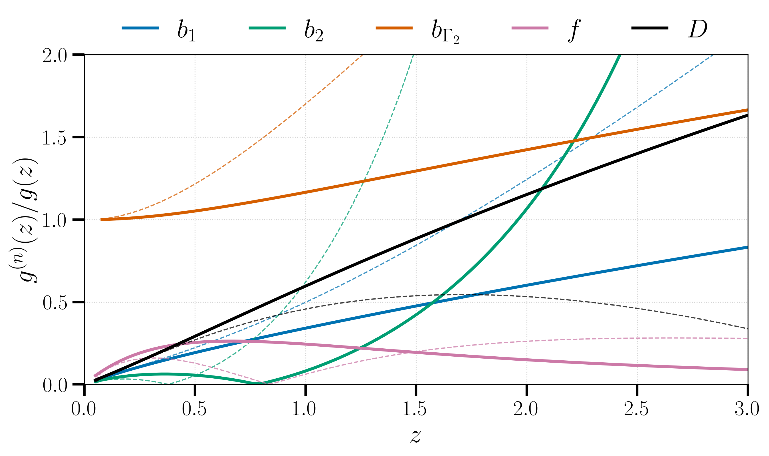
Figure 3: Ratios of redshift-dependent parameters with its first- (solid lines) and second-order (dashed) derivatives with respect to $\ln d$, as a function of redshift. In this figure, we take $b_{1}=\sqrt{1+z}$ as a proxy for the linear bias, with $b_{2}$ and $b_{\Gamma_{2}}$ given by Equations (4.9). The fiducial flat $\Lambda$CDM cosmology used to compute $f$ and $D$ is described in Section 4.

3.2 Derivation Overview

Starting from the local bispectrum in redshift space, Equation (2.22), we can use the series expansions shown in Equations (3.7) and (3.8) to reparameterise the $\bm{x}_{1},\bm{x}_{2}$ and $\bm{x}_{3}$ dependence in terms of $\bm{d}$, and $\bm{x}_{13}$ and $\bm{x}_{23}$.

Since there is no $\bm{x}_{13},\bm{x}_{23}$ dependence in the real-space integrals for the zeroth-order term in the expansion, which corresponds to the locally homogeneous limit $\bm{x}_{1}=\bm{x}_{2}=\bm{x}_{3}=\hat{\bm{d}}$, these become delta functions $\delta_{D}(\bm{q}_{1}-\bm{k}_{1})$ and $\delta_{D}(\bm{q}_{2}-\bm{k}_{2})$; therefore, the plane-parallel, constant redshift local bispectrum reduces to the standard expression

$$B^{\rm loc,0}(k_{1},k_{2},k_{3},\mu_{1},\phi)=2Z_{1}(k_{1},\mu_{1})Z_{1}(k_{1},\mu_{2})Z_{2}(k_{1},k_{2},\mu_{3})P_{L}(k_{1})P_{L}(k_{2})+\text{perms}.$$ (3.9)

However, beyond the zeroth order and after expanding $\bm{x}_{13}$ and $\bm{x}_{23}$ into their Cartesian vector components $x_{13,x},\ldots,x_{23,z}$, we can collect powers of $\epsilon_{1}$ and $\epsilon_{2}$, which leads to

$$\begin{split}B^{\text{loc}}(k_{1},k_{2},k_{3},\mu_{1},\phi,d)=&\int_{\bm{q}_{1},\bm{q}_{2},\bm{x}_{13},\bm{x}_{23}}e^{-i(\bm{k}_{1}-\bm{q}_{1})\cdot\bm{x}_{13}}e^{-i(\bm{k}_{2}-\bm{q}_{2})\cdot\bm{x}_{23}}\\ &\quad\times\sum_{i_{x},i_{y},i_{z}}\epsilon_{1}^{(i_{x}+i_{y}+i_{z})}\left[\left(\frac{x_{13,x}}{x_{13}}\right)^{i_{x}}\left(\frac{x_{13,y}}{x_{13}}\right)^{i_{y}}\left(\frac{x_{13,z}}{x_{13}}\right)^{i_{z}}\right]\\ &\quad\times\sum_{j_{x},j_{y},j_{z}}\epsilon_{2}^{(i_{x}+i_{y}+i_{z})}\left[\left(\frac{x_{23,x}}{x_{23}}\right)^{i_{x}}\left(\frac{x_{23,y}}{x_{23}}\right)^{i_{y}}\left(\frac{x_{23,z}}{x_{23}}\right)^{i_{z}}\right]\\ &\quad\times\mathcal{C}_{i_{x},i_{y},i_{z},j_{x},j_{y},j_{z}}(\bm{q}_{1},\bm{q}_{2},\bm{q}_{3},\bm{d}),\end{split}$$ (3.10)

where $\mathcal{C}_{i_{x},i_{y},i_{z},j_{x},j_{y},j_{z}}(k_{1},k_{2},k_{3},\mu_{1},\phi)$ are the bispectrum coefficients for each term in the expansion. Here, $i_{x},i_{y},i_{z},j_{x},j_{y},j_{z}$ correspond to the power of each respective Cartesian component of $\bm{x}_{13}\,\&\,\bm{x}_{23}$, and $n=i_{x}+i_{y}+i_{z}+j_{x}+j_{y}+j_{z}$ is the order of the expansion. In the $n=0$ case, $\mathcal{C}_{0,0,0,0,0,0}$ is just the standard zeroth-order bispectrum as in Equation (3.9):

$$\mathcal{C}_{0,0,0,0,0,0}\left(\bm{k}_{1},\bm{k}_{2},\bm{k}_{3},\bm{d}\right)=2Z_{1}(\bm{k}_{1},\bm{d})Z_{1}(\bm{k}_{2},\bm{d})Z_{2}(\bm{k}_{1},\bm{k}_{2},\bm{d})P_{L}(k_{1})P_{L}(k_{2})+\text{perms}.$$ (3.11)

For $n>0$, one can remove the $\bm{x}_{13},\bm{x}_{23}$ dependence in the real-space integrals by considering the Fourier relation

$$\frac{\partial}{\partial k_{j}}F(\bm{k})=-i\int\mathrm{d}^{3}\bm{x}\,\,e^{-i\bm{k}\cdot\bm{x}}x_{j}f(\bm{x}),$$ (3.12)

such that the Cartesian components of $\bm{x}_{13}\,,\,\bm{x}_{23}$ can be replaced with their derivatives, i.e. $x_{13,j}\rightarrow-i\partial_{k_{1,j}}$ and $x_{23,j}\rightarrow-i\partial_{k_{2,j}}$, acting on the whole expression. Therefore, the $\bm{x}_{13}$ and $\bm{x}_{23}$ integrals, as in the locally homogeneous limit, become Dirac-deltas $\delta_{D}(\bm{q}_{1}-\bm{k}_{1})$ and $\delta_{D}(\bm{q}_{2}-\bm{k}_{2})$.

Therefore, Equation (3.10) can be rewritten in the form

$$\begin{split}B^{\rm loc}(k_{1},k_{2},k_{3},\mu_{1},\phi;d)=\sum_{n}\left(\frac{i}{d}\right)^{n}\,\,\,\sum^{i_{x}+i_{y}+i_{z}+j_{x}+j_{y}+j_{z}=n}_{i_{x},i_{y},i_{z},j_{x},j_{y},j_{z}}&\left(\partial^{i_{x}}_{k_{1,x}}\partial^{i_{y}}_{k_{1,y}}\partial^{i_{z}}_{k_{1,z}}\right)\left(\partial^{j_{x}}_{k_{2,x}}\partial^{j_{y}}_{k_{2,y}}\partial^{j_{z}}_{k_{2,z}}\right)\\ &\times\mathcal{C}_{i_{x},i_{y},i_{z},j_{x},j_{y},j_{z}}\left(\bm{k}_{1},\bm{k}_{2},\bm{k}_{3},\bm{d}\right)\end{split}$$ (3.13)

such that there are $n$ partial derivatives acting on each coefficient for each term in the series.

Using Equation (3.13), we can collect terms at each expansion order, which are suppressed by a factor of $i/(k\,d)$. Therefore, if we separate wide-angle and radial-redshift terms as well as the Newtonian and relativistic contributions, we can express the bispectrum as a series of terms some suppression factors,

$$B^{\rm loc}= \left(\frac{i}{k\,d}\right)(B_{{\rm WA}_{1}}+B_{{\rm RR}_{1}})+\frac{i\,{\cal H}}{k}B_{{\rm GR}_{1}}+\left(\frac{i}{k\,d}\right)^{2}(B_{{\rm WA}_{2}}+B_{{\rm RR}_{2}}+B_{{\rm WA}_{1}{\rm RR}_{1}})$$ (3.14)

$$+\frac{i\,{\cal H}}{k}\left(\frac{i}{k\,d}\right)(B_{{\rm WA}_{1}{\rm GR}_{1}}+B_{{\rm RR}_{1}{\rm GR}_{1}})+\left(\frac{i\,{\cal H}}{k}\right)^{2}B_{{\rm GR}_{2}}$$

where we have truncated terms that are suppressed by ${\cal O}(1/k^{3})$ and higher. The theoretical multipoles induced by wide separations, for a given survey, can then be retrieved from the full local expression, as in Equation (2.7). Here, the imaginary first-order terms have odd powers of $\mu$ and therefore enter into the odd multipoles, while the real second-order terms are of even parity.

4 Results and Discussion

Our main results are the complete expressions for the local tree-level bispectrum, Equation (3.14), including wide-angle, radial-redshift and relativistic projection effects up to second order for a generalised LOS $\bm{d}$ (Section 3). For a typical analysis, this is decomposed into LOS multipoles and averaged over survey area (see Section 2). Because the full analytic expressions are extremely long and cumbersome, we do not show them here. Instead, we plot multipoles of the bispectrum for some given shapes and scales, and provide a publicly code containing the expressions, along with a Mathematica notebook used to compute them .

At first order, our numerical results for the pure wide-angle bispectrum is in agreement with both [38] and [39]; however, at second order, we only find agreement with [39] when the comparison was possible.

To examine these effects, we consider a few different types of future galaxy surveys of different tracers and redshift ranges, a H$\alpha$ Euclid-like survey $(0.9<z<1.8)$, a DESI-like BGS $(0.05<z<0.6)$ and SKAO1 HI galaxy survey $(0<z<0.5)$ [64] as well as a futuristic Phase-2 survey, SKAO2, galaxy survey over $(0.1<z<2)$. We show the results for a flat $\Lambda$CDM cosmology with parameters taken from [65]: $h=0.6766,\,\Omega_{\rm b}h^{2}=0.02242,\,\Omega_{\rm c}h^{2}=0.11933,\,A_{s}=2.105\times 10^{-9},\,n_{s}=0.9665$.

We use these surveys as [66] provides readily available models of magnification, $\mathcal{Q}$, and evolution, $b_{e}$, bias which are important for the relativistic contributions. These are astrophysical parameters that are defined with respect to the luminosity cut for a flux limited survey,

$$b_{e}=-\frac{\partial\,{\rm ln}\,n_{g}}{\partial\,{\rm ln}(1+z)},\,\,\mathcal{Q}=-\frac{\partial\,{\rm ln}\,n_{g}}{\partial\,{\rm ln}\,L}\bigg{|}_{c},$$ (4.1)

where $L$ is the luminosity function, $n_{g}$ is the comoving number density and $|_{c}$ refers to an evaluation at the flux cut. Fitting functions of evolution and magnification bias (as well as the number density) are derived from an assumed luminosity function for a given tracer and survey (see [66] for full details).

We assume the linear clustering bias is independent of luminosity [67]

$$\frac{\partial b_{1}}{\partial\,{\rm ln}\,L}\Big{|}_{c}=0.$$ (4.2)

For an H$\alpha$ Euclid-like survey, we assume a 15,000 $\rm{deg}^{2}$ footprint with a linear bias [67],

$$b_{1}(z)=0.9+0.4z,$$ (4.3)

and for magnification $\mathcal{Q}$ and evolution $b_{e}$ biases we adopt Model 3 from [66], such that,

$$\mathcal{Q}(z) =0.583+2.02z-0.568z^{2}+0.0411z^{3},$$ (4.4a)

$$b_{e}(z) =-7.29+0.470z+1.17z^{2}-0.0290z^{3},$$ (4.4b)

which is valid over the redshift range $(0.9<z<1.8)$.

For the 15,000 $\rm{deg}^{2}$ Bright Galaxy Sample (BGS) with DESI like specifications, we assume a linear bias [6]

$$b_{1}(z)=1.34/D(z),$$ (4.5)

with magnification $\mathcal{Q}$ and evolution $b_{e}$ biases [66],

$$\mathcal{Q}(z) =0.282+2.36z+2.27z^{2}+11.1z^{3},$$ (4.6a)

$$b_{e}(z) =-2.25-4.02z+0.318z^{2}-14.6z^{3},$$ (4.6b)

valid over the redshift range $(0.05<z<0.6)$.

For the 5,000 $\rm{deg}^{2}$ SKAO1 HI galaxy survey, we use a linear bias model from [68, 13]

$$b_{1}(z)=0.616\,\rm{e}^{1.0117\,z},$$ (4.7)

and similarly for the 30,000 $\rm{deg}^{2}$ SKAO2:

$$b_{1}(z)=0.554\,\rm{e}^{0.783\,z}.$$ (4.8)

Expressions for evolution and magnification biases as well as the number densities are interpolated from Table 1 and Table 2 in [66].

Then for simplicity in our modelling we assume the local Lagrangian expression for $b_{\gamma_{2}}$ and the quadratic fit for $b_{2}$ [69]:

$$b_{\Gamma_{2}} =-\frac{2}{7}(b_{1}(z)-1),$$ (4.9a)

$$b_{2} =0.412-2.143b_{1}(z)+0.929b_{1}^{2}(z)+0.008b_{1}^{3}(z)+4/3\,b_{\Gamma_{2}}(z).$$ (4.9b)

We plot the bispectrum for differing choices of LOS. For the results of the monopole we use a COM LOS ($r=s=1/3$) as this allows for a more accurate representation of wide-separation effects (see discussion in Section 4.1) while for the other multipoles, where unspecified, we use $\bm{d}=\bm{x}_{3}$ ($r=s=0$) as a default choice as an end-point LOS has a more simple connection to the standard FFT estimators used to measure the multipoles of the bispectrum. The $\bm{x}_{2}$ and $\bm{x}_{3}$ end-points are equivalent if the respective $k$-vectors also switch, i.e. $B_{\ell}(k_{1},k_{2},k_{3};\bm{x}_{2})\equiv B_{\ell}(k_{1},k_{3},k_{2};\bm{x}_{3})$; but this symmetry is broken for the $\bm{x}_{1}$ case for $\ell>0$ due to the fact that the multipole expansion is about $\bm{k}_{1}$.

For plots over fixed triangle shapes and scales, we choose three different triangle configurations:

• Equilateral: $k_{1}=k_{2}=k_{3}=0.01\>[h/{\rm Mpc}]$

• Folded: $k_{1}=2\,k_{2}=2\,k_{3}=0.02\>[h/{\rm Mpc}]$

• Squeezed: $k_{1}=k_{2}=10\,k_{3}=0.05\>[h/{\rm Mpc}]$

which are used in the plots below.

4.1 Line-of-sight dependence

Monopole

The monopole of the bispectrum corresponds to the case where we have averaged over the LOS dependence, $\mu_{1},\phi$. Therefore, it is not decomposed with respect to any LOS and as such there is no LOS dependence in our estimator; in our theory however, we still have to define a point from which to Taylor expand about to describe our configuration space triangle and therefore our LOS dependent describe the choices of points about which to do the expansion.

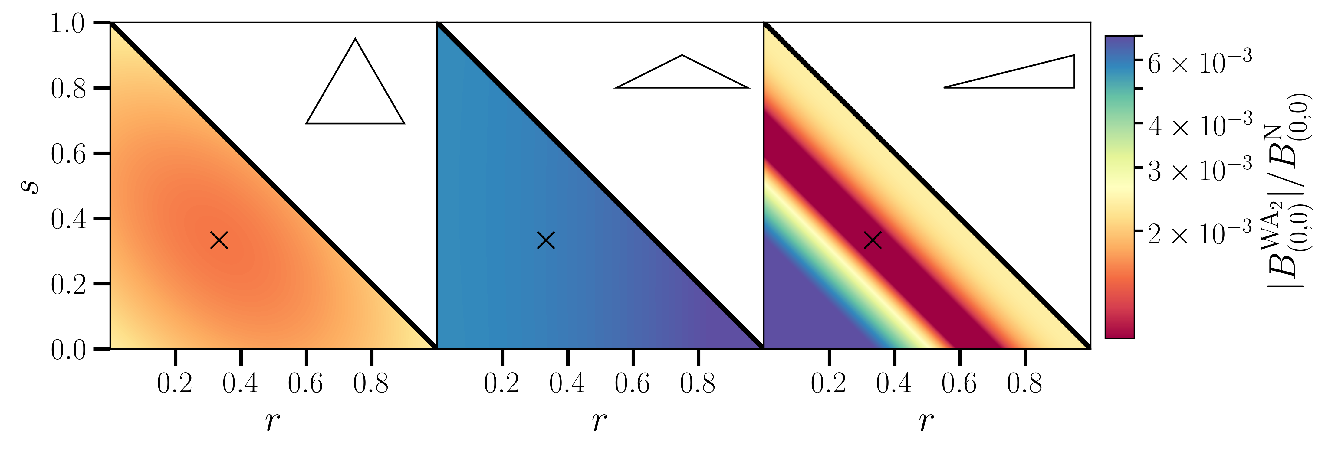
Figure 4: Fractional contribution to the monopole from second-order wide-angle effects, $B^{{\rm WA}_{2}}_{(0,0)}$, for a H$\alpha$ Euclid-like survey at redshift $z=1$. This is plotted over different LOS directions in the configuration space triangle (see Figure 2), for three fixed triangles: equilateral (left), folded (middle) and squeezed (right). The corners of the triangles represent the end-point lines-of-sight: $\bm{x}_{1}$ (bottom right), $\bm{x}_{2}$ (top left), and $\bm{x}_{3}$ (bottom left). The COM LOS is denoted by $\times$.

For the monopole only the even order wide-separation and relativistic terms enter and so in this case we are referring purely to the second order terms. Figure 4 shows the $r,s$ (which parameterise our choice of LOS) dependence of the monopole for different bispectrum shapes. For the equilateral shape, $k_{1}=k_{2}=k_{3}$, all three end-points are equivalent however for a non-endpoint LOS, for example the centre-of-mass (COM) where $r=s=1/3$, will generally induce a smaller contribution. This can be explained if we consider the configuration space triangle, Figure 2; the separations between $\bm{d}$ and the end-points are less extreme for a point in the centre of the triangle. Thus, the wide-separation series expansions in terms of $A_{i}\epsilon_{1},B_{i}\epsilon_{2}$ should converge quicker, and therefore a COM LOS should be more accurate to the true non-linear wide-separation corrections that we observe. Therefore, for all discussion of the monopole, we use a COM LOS.

Outside the equilateral configuration, wide-separation effects are often weighted more if the LOS choice is weighted more towards an end-point which corresponds to a smaller $k$-vector; wide-separation effects are larger when the scales that are correlated are larger.

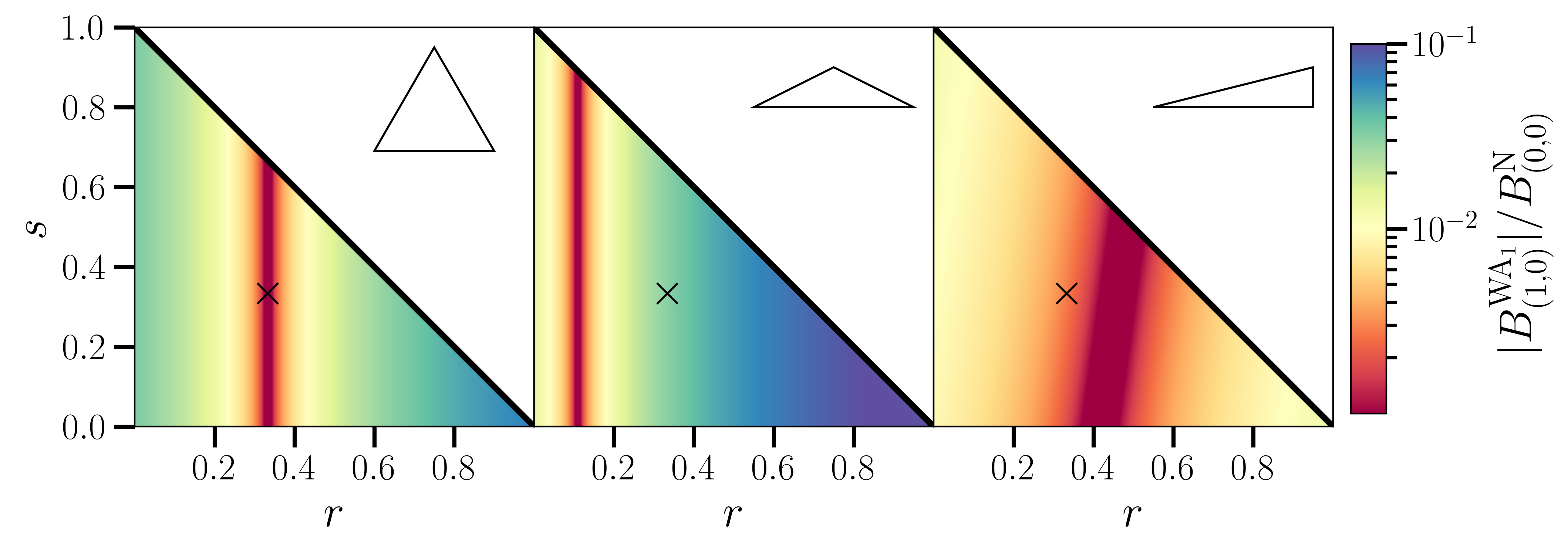
(a) Wide-angle (WA) contribution.

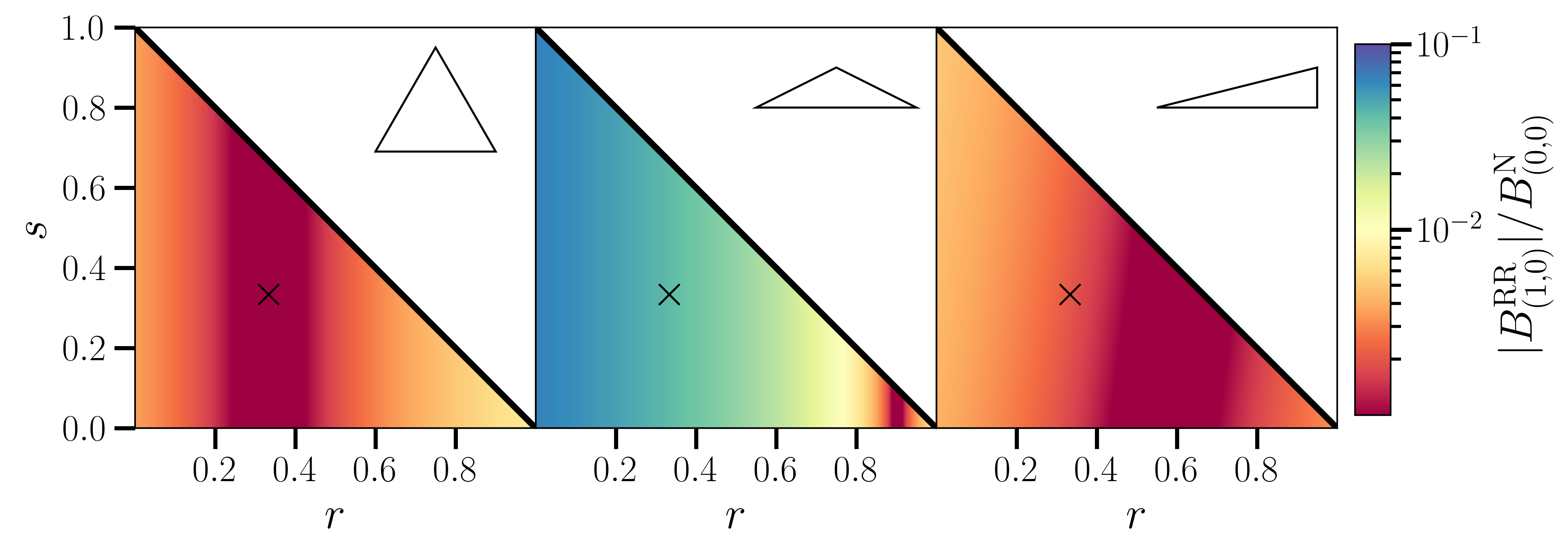
(b) Radial-redshift (RR) contribution.

Figure 5: Contribution to the dipole as a fraction of the monopole from first-order wide-separation effects for a Euclid-like H$\alpha$ survey at $z=1$. This is plotted over LOS choices (parameterised by $r$ and $s$, as in Equation 3.2) in configuration space, for three fixed triangles: equilateral (left), folded (middle) and squeezed (right). The corners of the triangles represent the end-point LOS: $\bm{x}_{1}$ (bottom right), $\bm{x}_{2}$ (top left), and $\bm{x}_{1}$ (bottom left). The COM LOS is denoted by $\times$.

Other multipoles

For any $\ell\neq 0$ multipole, the choice of LOS is more complex as is it not only the point about which we expand from to describe the configuration space triangle, but also it is the vector with which we use to define our spherical harmonic basis. Figure 5 shows the odd wide-separation contributions (both radial redshift and wide angle) to the bispectrum dipole as a function of $r,s$. First order wide-separation terms are linear in the expansions parameters and so there is no $r,s$ dependence from the convergence in the equilateral limit, but as before different $k$ generate $r,s$ dependence due to the loss of symmetry (for this folded configuration $k_{2}=k_{3}$ and therefore there is no change with respect to $s$). But outside the monopole there is a dependence on $r$ as our spherical harmonics are defined with respect to $\hat{\bm{k}}_{1}$. For the case of non-zero $m$ multipoles these also contain information about $k_{2}$ and therefore these have additional $s$ dependence.

4.2 Parity odd

The imaginary contributions coming from odd moments is composed of the first-order contributions from the three different effects: wide-angle, radial-redshift and relativistic terms:

$$B^{(1)}_{\rm loc}=B_{\rm WA_{1}}+B_{\rm RR_{1}}+B_{\rm GR_{1}}.$$ (4.10)

These will enter the odd multipole moments of the bispectrum, namely $B_{10}$. We show each of these contributions, and the total bispectrum, in Figure 6, after integrating over all possible LOS.

At first order in the wide-separation series expansion, the contributions are linear in the expansion parameters and, therefore, any choice of LOS in the configuration-space triangle can be expressed as the linear combination of the three end-point lines-of-sight:

$$B^{(1)}(k_{1},k_{2},k_{3},\mu_{1},\phi,d;\bm{d})= rB^{(1)}(k_{1},k_{2},k_{3},\mu_{1},\phi,d;\bm{x}_{1})+sB^{(1)}(k_{1},k_{2},k_{3},\mu_{1},\phi,d;\bm{x}_{2})$$ (4.11)

$$+(1-r-s)B^{(1)}(k_{1},k_{2},k_{3},\mu_{1},\phi,d;\bm{x}_{3}).$$

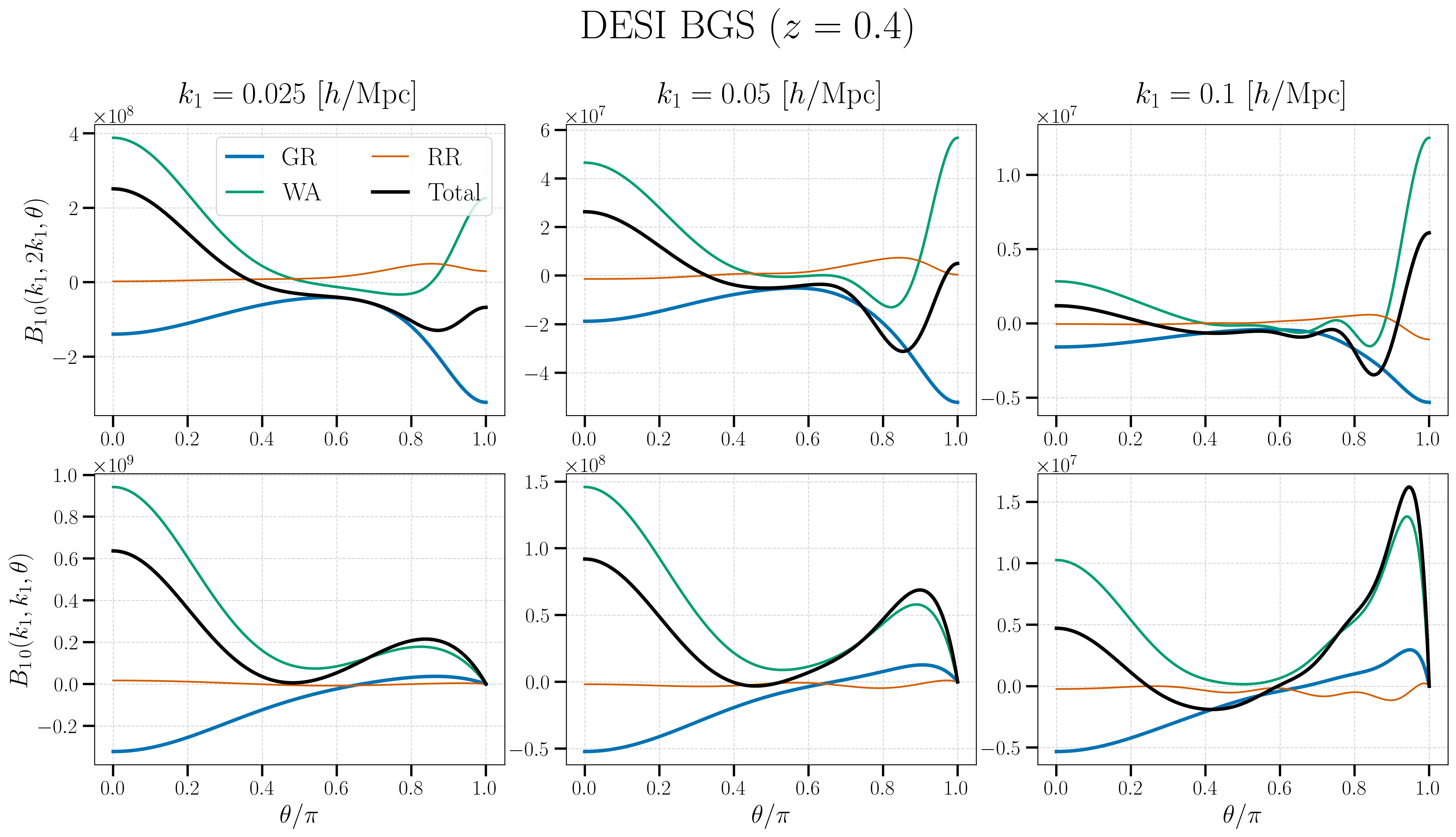
Figure 6: Dipole moment $\ell=1$ ($m=0$) of the bispectrum for $k_{2}=2k_{1}$ (top) and the isosceles configuration, $k_{1}=k_{2}$ (bottom), as a function of the angle between $k_{1}$ and $k_{2}$. The results assume a DESI-like Bright Galaxy Survey (BGS) at redshift $z=0.4$. Each panel displays the general relativistic (GR, blue), wide-angle (WA, green), and radial-redshift (RR, orange) contributions to the bispectrum, and the total signal (black). The total bispectrum is computed from the sum of each of these contributions.

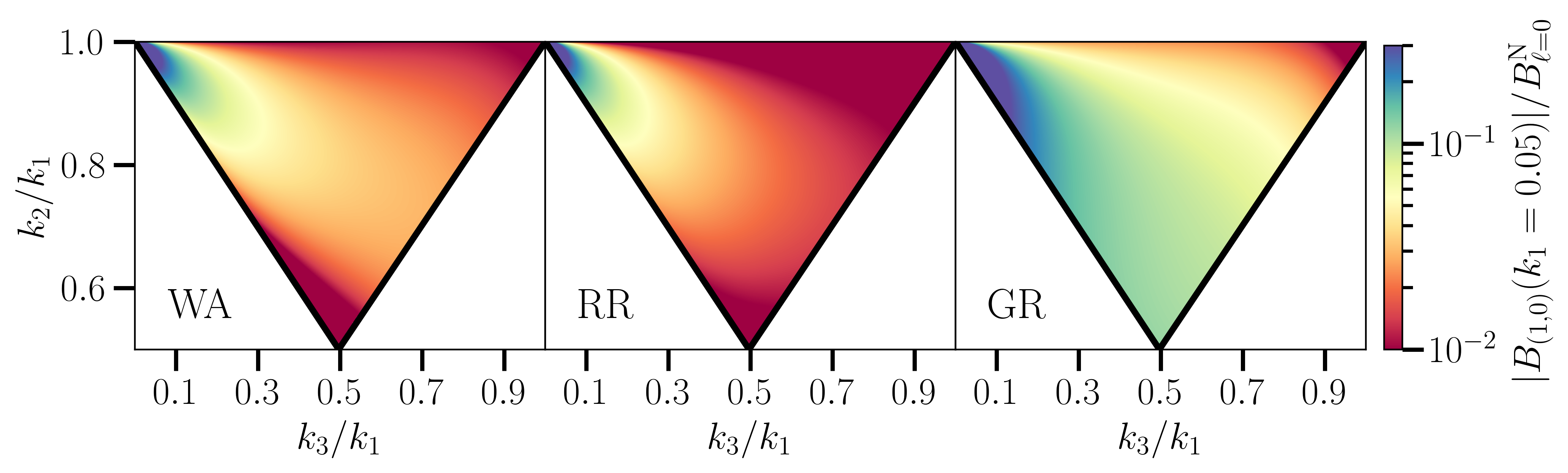
Figure 7: Contribution to the dipole as a fraction of the monopole from first order wide angle, radial redshift and relativistic effects for a H$\alpha$ Euclid-like survey at $z=1$. This is plotted over bispectrum shapes, for a fixed scale with $k_{1}=0.05\,\,[h/$Mpc]. Top left corner: Squeezed, Top right corner: Equilateral, Bottom: Folded.

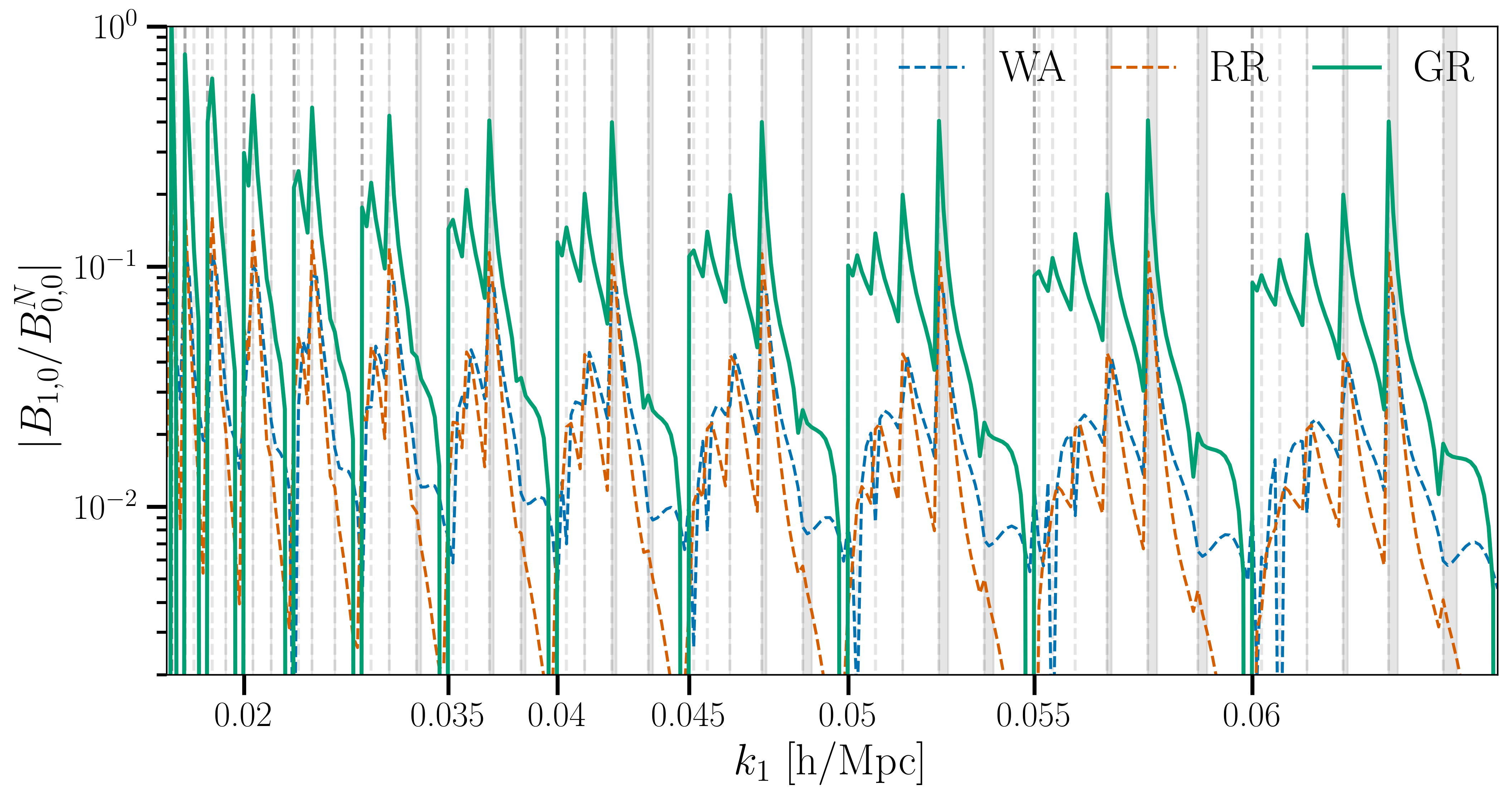
Figure 8: Odd parity first order contributions to the dipole as a fraction of the monopole plotted over all triangles, where $k_{1}>k_{2}>k_{3}$, for a Euclid-like H$\alpha$ survey at $z=1$. The plot represents all triangles in a nested structure where we use a bin width of $0.005\>[h/{\rm Mpc}]$. The thicker dashed lines represent a step in $k_{1}$ ($k_{2}$ (and $k_{3}$) reset to their minimum value for that $k_{1}$ considering the triangle condition), such that it is constant in that region between dashed lines. Folded triangles occur on these dashed lines, with equilateral triangles directly before it. The fainter dashed lines denote the corresponding steps in $k_{2}$. The shaded regions represent ‘squeezed’ regions where $3\,k_{3}<k_{2}\leq k_{1}$.

As expected due to their $1/k$ suppression, Figure 7 and Figure 8 shows the signal for all three effects increases at large scales with peaks in the squeezed limit, corresponding to a small $k_{3}$ in this case. A notable result here is that relativistic effects are in general larger than their wide-separation counterparts (note for a single tracer in the equilateral case the relativistic effects are zero due to the symmetry), unlike in the power spectrum, though we stress the relativistic terms are heavily dependent on the models of evolution and magnification bias. Wide-separation effects can also lead to higher powers of $\mu$ and as such it has the effect of moving signal into the higher multipoles and therefore for higher $\ell$, wide-separation effects will generally have a greater fractional contribution to the overall signal. We include plots of the contributions for other odd multipoles in Appendix C.

The wide angle contribution has a $1/(kd)$ suppression and therefore it is less important at high redshifts, as shown in Figure 9. However for the BGS, at low redshifts, they can dominate the dipole signal, though at a certain redshift and scale, given by $k=2\pi/\chi(z)$, the wide-separation perturbative expansion will break down (represented by the vertical dashed vertical lines in Figure 9).

First-order radial-redshift contributions however, if we use derivatives with respect to redshift, scale as $\mathcal{H}/k$. Therefore, for surveys covering a higher redshift range, such as the Roman Space Telescope [9], or the proposed Stage-V MegaMapper survey [70], we would expect the wide-angle contribution to be negligible, while the radial-redshift corrections would still need to be considered for precision analyses.

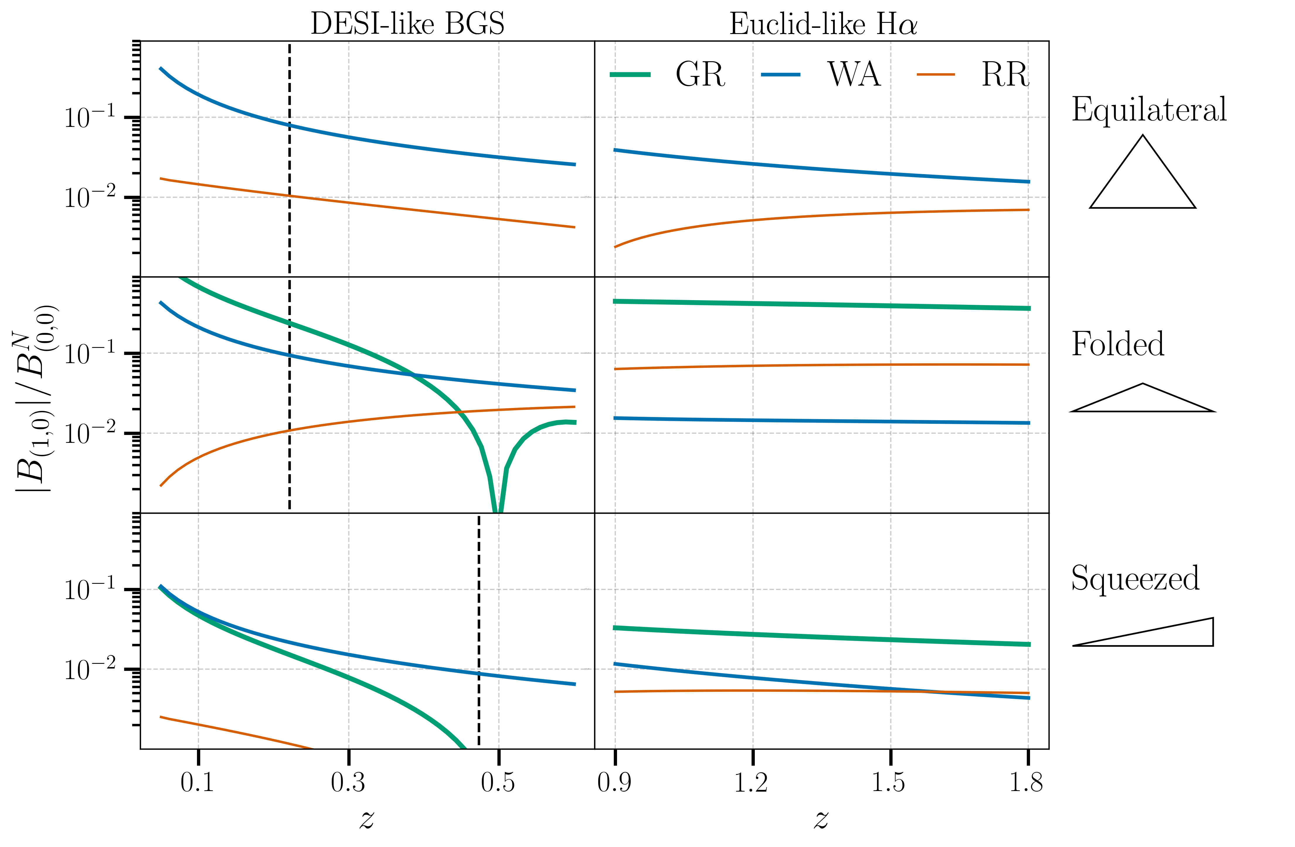
Figure 9: Odd parity first-order contributions to the dipole as a fraction of the monopole for three different triangle configurations (equilateral, squeezed and folded) for both a DESI BGS and an H$\alpha$ Euclid-like survey. The dashed vertical represent the redshift at which the wide-separation expansion is expected to break down for the given scales.

4.2.1 Signal-to-noise ratio

To consider the detectability of these effects in future surveys we compute the signal-to-noise ratio (SNR) for the dipole of the bispectrum:

$${\rm SNR}^{2}=\sum_{\triangle}\frac{B_{\ell m}(k_{1},k_{2},k_{3})B_{\ell m}^{*}(k_{1},k_{2},k_{3})}{{\sf C}_{\ell m}(k_{1},k_{2},k_{3})}$$ (4.12)

where we discretely sum over all triangles $\triangle$ where $k_{1}>k_{2}>k_{3}$. We assume a Gaussian bispectrum covariance for simplicity with the expressions given in Appendix B.

We compute the SNR in redshift bins of width $\Delta z=0.1$ and then the cumulative SNR for a given survey is given by summing the SNR from each bin in quadrature ${\rm SNR}(<z)=\sum_{z}\sqrt{{\rm SNR}(z)^{2}}$. In $k$-space we impose bin widths of $\Delta k=2k_{f}$ where $k_{f}$ is the fundamental frequency of the survey ($k_{f}\approx(2\pi)/V^{1/3}$) and a cut-off scale at $k_{max}=0.1\>[h/{\rm Mpc}]$. We also exclude Fourier modes where $k>2\pi/x(z_{\rm min})$ for the minimum redshift of the bin as the wide angle expansion breaks down. Results are plotted in Figure 10 and SNR values are given in Table 1.

	DESI BGS	Euclid H$\alpha$	SKAO1	SKAO2
${\rm SNR}_{\rm WA}$	1.9	1.9	1.2	5.5
${\rm SNR}_{\rm RR}$	0.3	2.4	0.1	2.5
${\rm SNR}_{\rm WS}$	1.6	1.1	1.2	5.9
${\rm SNR}_{\rm GR}$	1.8	11.7	0.4	8.8
${\rm SNR}_{\rm All}$	2.8	10.9	1.3	13.1

Table 1: SNR for the dipole, $\ell=1,m=0$, of the galaxy bispectrum for different contributions for each survey we consider.

We note that this analysis ignores several key factors and just constitutes a crude calculation. Firstly, these results will be heavily impacted by the convolution with the survey window function which will dampen the signal on the large scales as well as mix the odd and even parity signals. On smaller, mildly non-linear scales the tree level theory assumed here will be inadequate both in the signal and the covariance. In general much more attention needs to paid to the covariance; the Gaussian covariance limit has shown to be a poor approximation to the true covariance, particularly in the squeezed limit [71, 72, 73], and also we neglected the relativistic and wide-separation contributions. Lastly, proper consideration of small scales should allow for higher $k_{\rm max}$ allowing a greater range of mode to be accessed rather than the harsh cut-off of $k_{\rm max}=0.1\>[h/{\rm Mpc}]$ considered here. These results do however appear broadly consistent with those of previous analyses [67, 38].

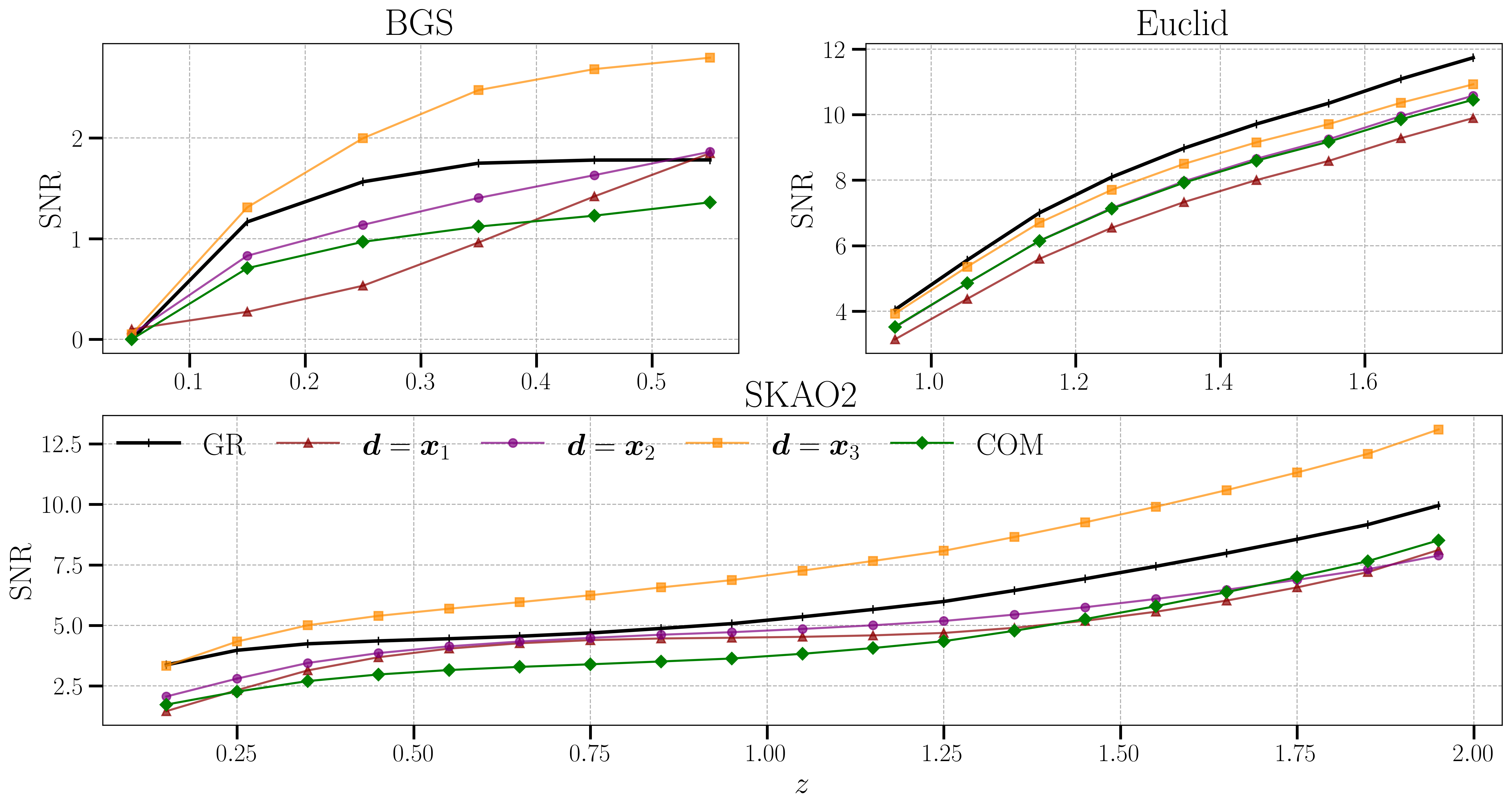
Figure 10: Cumulative SNR of the dipole, $(\ell=1,m=0)$ plotted over redshift bins, for the three different surveys we consider, without wide-separation effects (green) – that is, purely relativistic contribution – and with wide-separation for different LOS choices.

The SNR is strongly dependent on survey volume for all three contributions as larger volumes leads to a smaller $k_{f}$ and, therefore, more $k$-modes. The predominant part of the signal arises from squeezed, or moderately squeezed triangles, where $k_{3}$ is small and $k_{1}$ and $k_{2}$ are comparatively large. The low redshift samples of DESI BGS and SKAO1-like samples do not cover a large enough volume for a strong detection of the relativistic signal while for the larger redshift coverage of SKAO2 and Euclid, we obtain ${\rm SNR}\sim\mathcal{O}(10)$. Therefore, one would expect the relativistic terms to be detectable in other similar spectroscopic surveys, like the higher redshift ELG and LRG samples of DESI. For a cosmic variance limited survey, with $f_{\rm sky}=1$ and assuming $b_{e}=\mathcal{Q}=0$, as shown in Figure 11, also has an ${\rm SNR}\sim\mathcal{O}(10)$ for the relativistic signal. The dominant non evolution and magnification bias terms generally are inversely proportional to redshift, however for a realistic survey, non-zero evolution and magnification biases will drive the relativistic signal at higher redshifts.

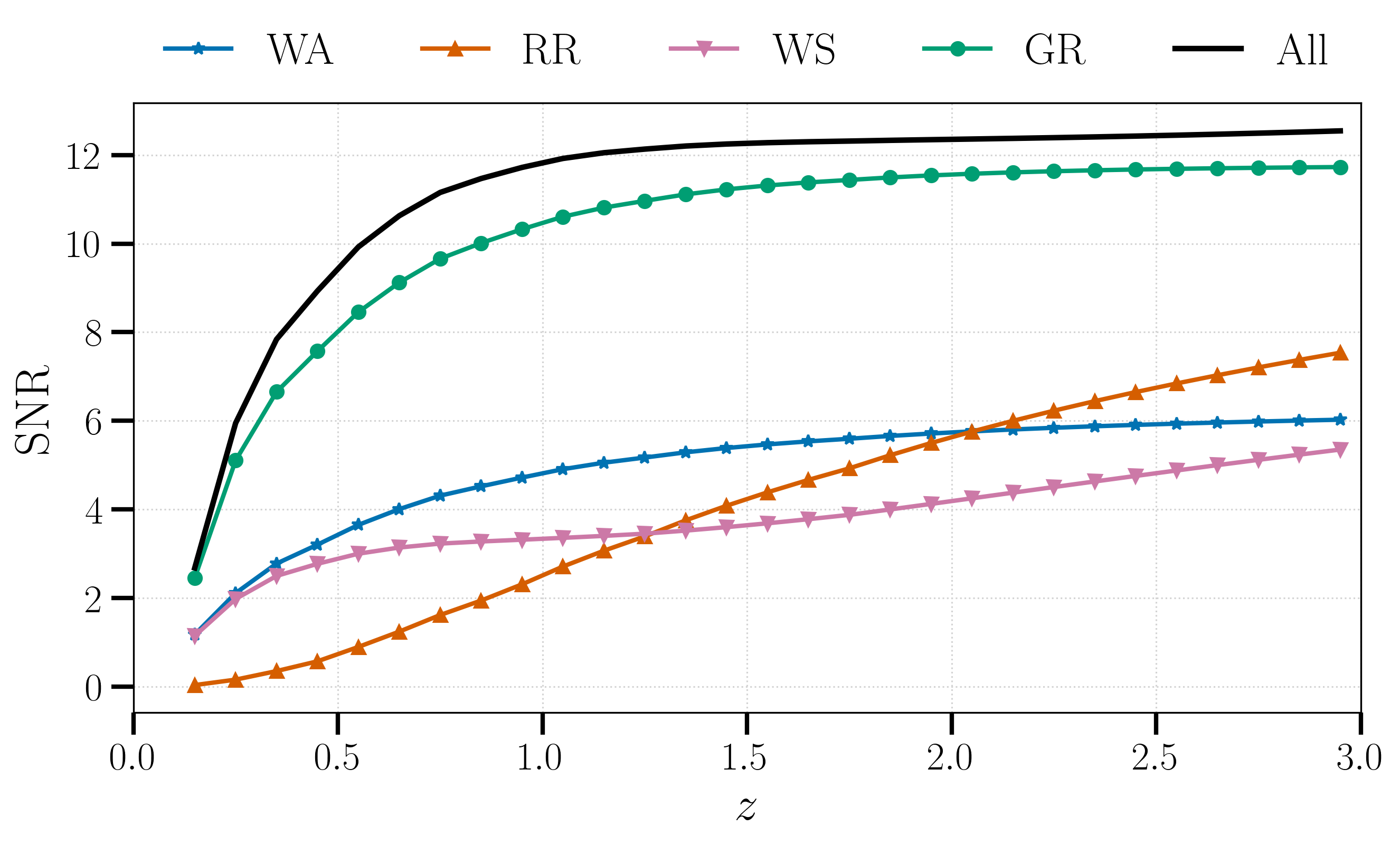
Figure 11: Cumulative SNR for different contributions to the dipole of the bispectrum for a cosmic variance limited survey with $b_{e}=\mathcal{Q}=0$. Also $b_{1}=\sqrt{1+z}$ and $b_{2}$ and $b_{\Gamma_{2}}$ are set by Equation (4.9).

Therefore, for a realistic analysis as well as accessing more modes by pushing to higher redshifts, greater constraining power on relativistic corrections should be achievable with multi-tracer approaches (e.g. see [74] for example os constraints from a multi-tracer analysis); indeed in the $(\mathcal{H}/k)$ relativistic corrections enter the odd multipoles of the power spectrum for the multi-tracer case.

Further, while we just just considered the dipole, $\ell=1,m=0$, for the discussion here, additional information from the imaginary bispectrum is contained in the other odd multipoles.

Confident detection of the wide-separation corrections requires large volumes, but as expected the wide angle signal peaks at lower redshifts while the radial redshift signal is fairly redshift independent. Their effect on the overall SNR of the dipole, as shown in figure 10, is survey dependent and is also dependent on the LOS choice.

If we consider the linear-order expansions in Equations (3.7) and (3.8), then the wide-angle terms contain either the dot products $\bm{d}\cdot\hat{\bm{x}}_{1i}$, or $\bm{k}\cdot\hat{\bm{x}}_{1i}$, and the radial-redshift terms have a factor of $\bm{d}\cdot\hat{\bm{x}}_{1i}$. In general, these $\bm{d}\cdot\hat{\bm{x}}_{1i}$ terms appear more suppressed for a less extreme LOS choice; often, as in the Euclid-like case, the $\bm{d}\cdot\hat{\bm{x}}_{1i}$ and $\bm{k}\cdot\hat{\bm{x}}_{1i}$ contributions are of opposite sign and, therefore, the wide-angle contributions are larger for a COM LOS as there is less cancellation between the two contributions.

Fisher forecast

If we introduce amplitude parameters for each effect ($\alpha_{\rm GR},\alpha_{\rm WA},\alpha_{\rm RR}$), such that the odd part of the bispectrum is given by

$$B^{(1)}_{\rm loc}=\alpha_{\rm WA}B_{\rm WA_{1}}+\alpha_{\rm RR}B_{\rm RR_{1}}+\alpha_{\rm GR}B_{\rm GR_{1}},$$ (4.13)

we can examine the degeneracy between the contributions by performing a Fisher matrix analysis on these parameters. Assuming a Gaussian likelihood, the Fisher matrix depends on the derivative of the multipoles with respect to the parameters:

$$F_{ij,\ell m}=\sum_{\triangle}\frac{\partial B_{\ell m}}{\partial\theta_{i}}{\sf C}^{-1}_{\ell m}\frac{\partial B_{\ell m}^{*}}{\partial\theta_{j}}.$$ (4.14)

Figure 12 shows the 1- and 2-$\sigma$ forecasted constraints on the amplitude parameters for the DESI-, Euclid-, and SKAO2-like surveys. For the Euclid case, the wide-separation and relativistic contributions are positively correlated, unlike in the SKAO2-like galaxy survey like case. We can see the shift in the correlations due to different ranges of redshift for each survey.

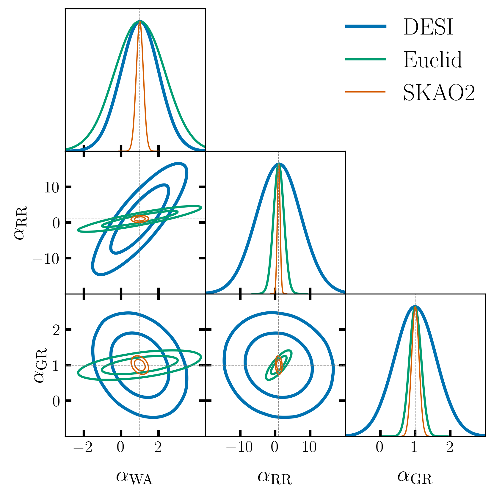
Figure 12: 1- and 2-$\sigma$ forecast for the amplitude parameters measured with the dipole of the bispectrum for a DESI BGS (thick blue), Euclid H$\alpha$ (green) and a SKAO2 HI (thin orange) galaxy surveys.

4.3 Parity even

The parity even part of the wide-separation, and relativistic corrections, which comes in at second order, includes a relativistic and wide-separation mixing contribution, such that we can write

$$B^{(2),{\rm loc}}=\left(\frac{i}{k_{i}\,d}\right)^{2}(B_{{\rm WS}_{2}})+\frac{i\,{\cal H}}{k_{i}}\left(\frac{i}{k_{i}\,d}\right)(B_{{\rm WS}_{1}{\rm GR}_{1}})+\left(\frac{i\,{\cal H}}{k_{i}}\right)^{2}B_{{\rm GR}_{2}},$$ (4.15)

where WS includes both wide-angle and radial-redshift contributions, as well as their mixing at second order.

As in the case of the odd parity terms, the even parity relativistic contribution, $({\rm GR}_{2})$, is generally larger than the wide-separation contributions (as in Figures 13 and Figure 13), $({\rm WA}_{2}+{\rm RR}_{2}+{\rm WA/RR})$ though at second order we also have the mixing contribution which is greater than the pure wide-separation contribution.

These second-order contributions are smaller than their first-order imaginary counterparts. The percentage correction of wide-separation effects (including the mixed terms) to the standard Newtonian term is $<1\%$ for most triangles, but it peaks on small scales and in the squeezed limit, where it can be of order $10\%$.

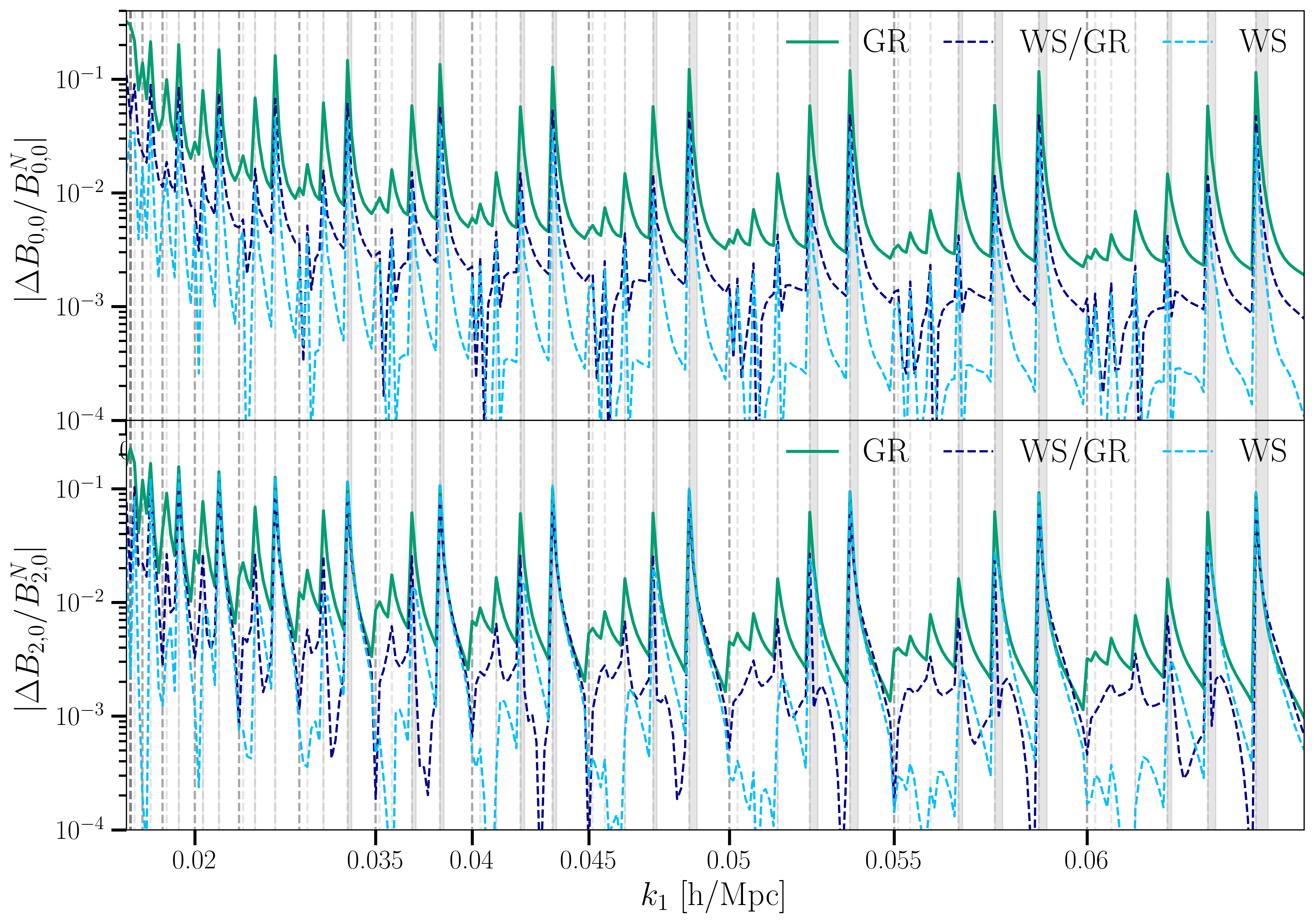
Figure 13: Fractional contribution to the monopole (top) and quadrupole (bottom) from wide-separation (WS) and relativistic effects (GR) and their mixing (WS/GR) for a H$\alpha$ Euclid-like survey at $z=1$, plotted over all triangles.

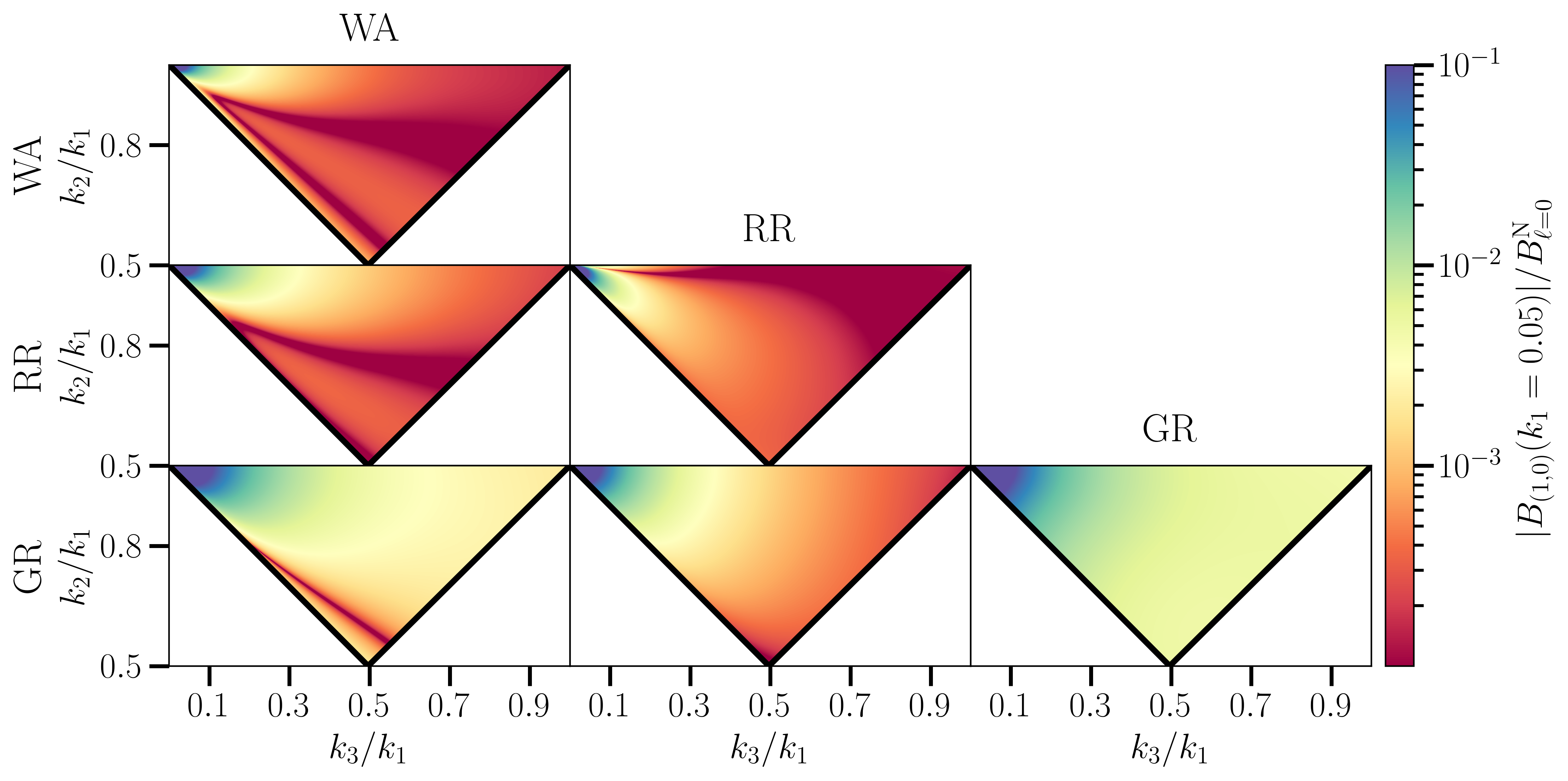
Figure 14: Fractional contribution to the monopole from wide-separation and GR effects for a H$\alpha$ Euclid-like survey at $z=1$. This is plotted over bispectrum shapes, for a fixed scale with $k_{1}=0.05\,\,[h/Mpc]$.

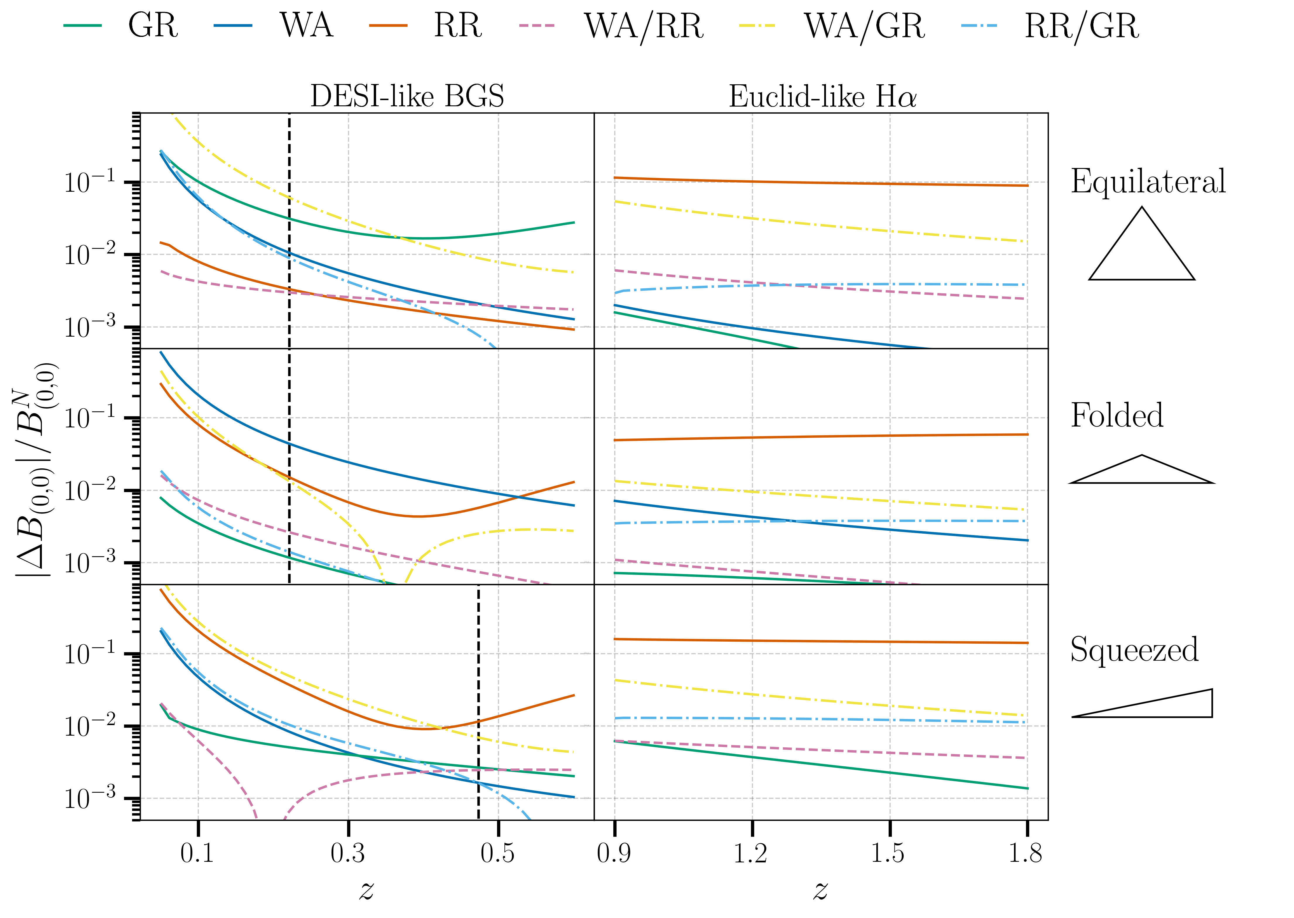
Figure 15: Even parity second-order contributions to the monopole as a fraction of the Newtonian part for three different triangle configurations (equilateral, squeezed and folded) for both a DESI BGS and an H$\alpha$ Euclid-like survey.

4.3.1 Effective primordial non-Gaussianity

While the percentage contributions of wide-separation corrections to the monopole are of order $<1\%$ for scales $k\approx 0.01\,[h/{\rm Mpc}]$, with a larger contribution coming from the mixing with the relativistic corrections, it is important to consider for an accurate analysis of PNG; if wide-separation and relativistic corrections are ignored in the theory modelling then this unaccounted for signal can mimic a PNG signal. Previous studies have shown that relativistic corrections can significantly bias measurements for PNG of the local type in the monopole of the galaxy bispectrum [75, 76], and here we consider a similar analysis with the inclusion of wide-separation corrections.

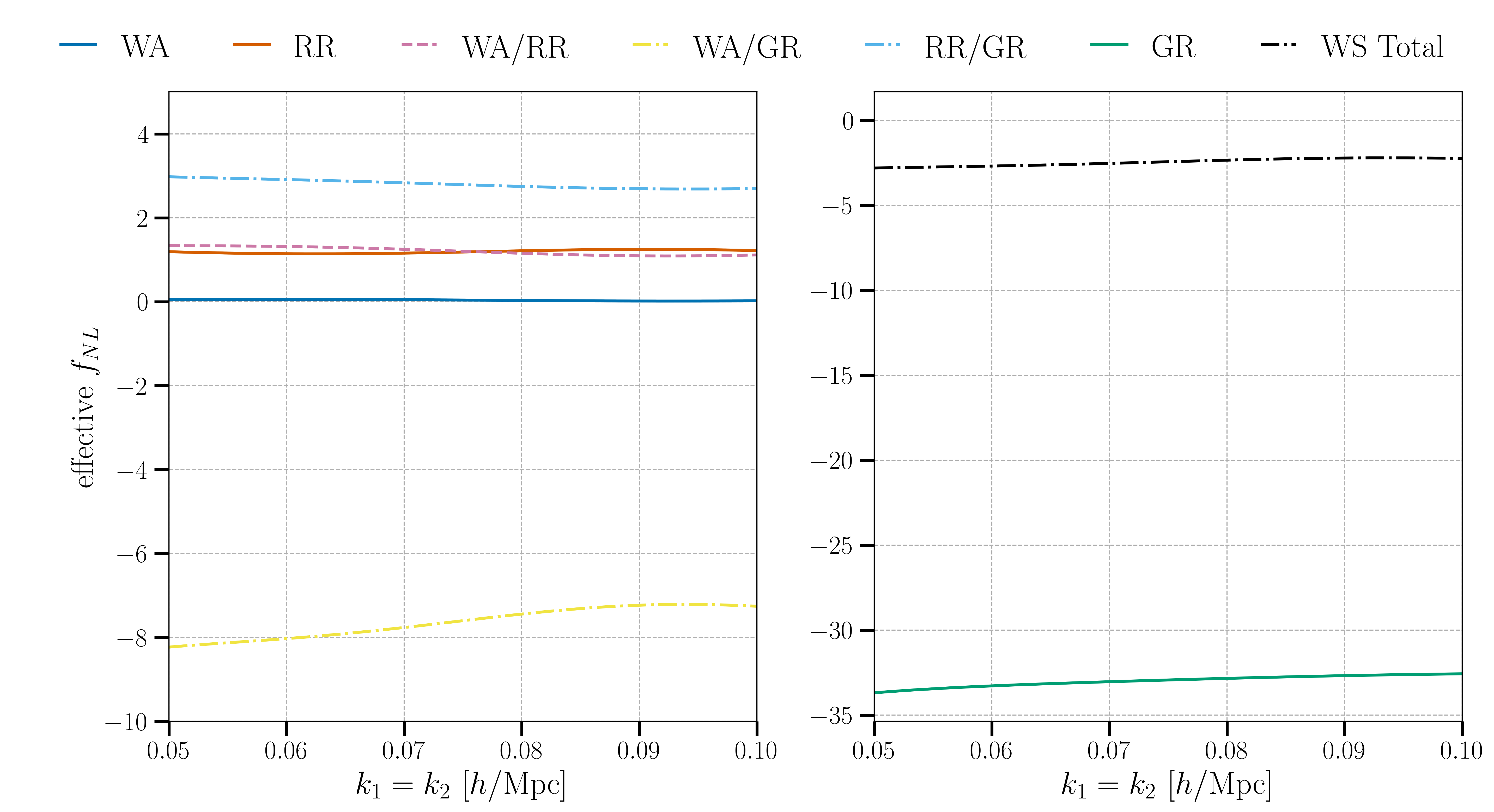
Figure 16: Left Panel: Effective local $f_{\rm NL}$ induced in the monopole by each wide-separation contribution (including mixing with relativistic terms) for a squeezed limit configuration with $k_{3}=0.01$, for a Euclid-like survey at $z=1$. A COM LOS is used for the monopole. Right Panel: Combined effective $f_{\rm NL}$ for all wide-separation effects alongside the pure relativistic contribution.

Focusing on local type PNG and as such we consider the squeezed limit of the bispectrum monopole at large scales. We consider a local PNG contribution including scale dependent bias following [77], with full details of our modelling given in Appendix D. The left panel of Figure 16 shows the effective local $f_{\rm NL}$ induced by each type of wide-separation correction, for the Euclid-like bias parameters at $z=1$. We can see that while the pure wide angle contribution mimics $f_{\rm NL}$ of $\mathcal{O}(0.1)$, which is consistent with the findings in [39], the contributions from the other terms are more significant. The relativistic/wide-separation mixing in particular can lead to the individual contributions with $f_{\rm NL}\approx 10$. The right panel shows the total wide-separation corrections, including all mixing terms, as well as the dominant pure relativistic term.

In comparison to previous results, the effective local non-Gaussianity induced by GR effects, $f^{\rm eff\,GR}_{\rm NL}$, is larger than that in [75, 76]. This can attribute this largely to the signal from the evolution and magnification bias terms. For $b_{\rm e}=\mathcal{Q}=0$, we find $f^{\rm eff\,GR}_{\rm NL}\approx 5$ roughly in line with the results of [75], who considered the impact of local relativistic projection effects on the full bispectrum. Detailed comparison with the results of [76] is not straightforward as they consider the bispectrum in a spherical basis. For a higher redshift sample, the wide-angle contribution will decrease (see Figure 15), but the radial-redshift contribution, in particular, will still be relevant for precision constraints.

Wide-separation corrections directly on PNG contribution (wide-separation/PNG mixed term) are negligible for most analyses; however, a full relativistic treatment of PNG is more subtle and requires further attention [78].

The effective $f_{\rm NL}$ induced by the wide-separation corrections in the galaxy bispectrum falls with current $f_{\rm NL}$ constraints, but in order to reach for example the goal of $\Delta f_{\rm NL}\approx 1$, both wide-separation and relativistic corrections cannot be ignored.

5 Conclusions

In this work, we computed wide-separation effects to the three-dimensional galaxy bispectrum, with a generalised line-of-sight orientation in the triplet of galaxies including, for the first time, the contribution from local redshift evolution, which becomes relevant when galaxies are widely separated in terms of radial distance. The expressions and routines used to compute these effects for given kernels of the galaxy bispectrum are publicly available . For low redshifts and large angular footprints, the perturbative approach to wide-angle effects breaks down at the largest scales. However, this perturbative approach should be robust enough to make precision constraints for the most relevant scales in ongoing (DESI and Euclid) and future (SKAO2) surveys that map large redshifts.

We show that the imaginary part of these effects, which enter the odd multipole moments of the bispectrum, can be up to 10% of the Newtonian monopole for ongoing Stage-IV galaxy surveys, like Euclid (see Figure 8). At lower redshifts, the wide-angle (WA) contribution is larger for a DESI-like Bright Galaxy Survey (BGS), compared to the radial redshift (RR) contributions, but for $z>1$ they have a similar magnitude for the Euclid-like case considered here (Figure 9). We stress, nonetheless, the dependence of our results on the range of scales, shapes, redshifts and bias parameters considered.

We have compared these contributions to the signal from general relativistic corrections, including both dynamical and projection effects. These contributions are, in general, larger than the wide-separation terms for the cases considered here, and the leading-order imaginary part that enters the odd multipoles should be detectable with a single tracer in surveys with large enough volume: for a Euclid-like H$\alpha$ galaxy survey, over $0.9<z<1.8$, our forecast showed a signal-to-noise ratio of order 10. Since the odd multipoles of the galaxy bispectrum are an interesting method to constrain gravity on cosmological scales, in this work we have shown how important it is to accurately model and account for the wide-separation effects – including the radial redshift contribution – due to their degeneracy with the relativistic terms.

The second-order wide-separation effects are real and affect the even-parity multipoles. Here, we showed that these can mix with the relativistic signal, and the mixing terms between wide-separation and relativistic effects can be of similar order to the pure second-order relativistic signal. These effects, while percentage or sub-percentage level corrections to the Newtonian contribution, will still need to be considered for precision analysis on large scales ($k\lesssim 10^{-2}\,\,h/{\rm Mpc}$), which are particularly relevant to constrain primordial non-Gaussianities (PNG). For PNG of the local-type, we showed that wide-separation effects in the squeezed limit, if unaccounted for, can ‘mimic’ $f_{\rm NL}$ up to $\mathcal{O}(1)$ (Figure 16) mainly through the mixing with the relativistic terms. The effective $f_{\rm NL}$ we find generated by the pure relativistic term alone, $f_{\rm NL}\approx\mathcal{O}(30)$, is larger than in previous analysis, but this can be attributed to the models of evolution and magnification bias we use.

In this work, we omitted the effect of the convolution of the survey window function which significantly impact the large scales analysed, and therefore it is important to model how these contributions will be affected. The modelling of this is non-trivial, and we leave this aspect as an avenue of future work. Further, the impact of nonlinear linear effects should be considered, and the inclusion of mode-coupling, off-diagonal and beyond-Gaussian terms should be included in a realistic modelling of the covariance matrix.

Code Availability Statement

Routines used in this work are publicly available at https://github.com/craddis1/ws_bk_theory.

Appendix A Impact of the survey window convolution

The window function convolution will dampen the signal for $k$-modes that approach the size of the survey. Additionally, it introduces additional terms from the convolution, such that for a given term with $\mu^{m}$ dependence it introduces additional terms dependent on $\mu^{m-n}/k^{n}$. The effect of this is to mix the parity odd and even terms such that different signals enter each multipole, though this is suppressed on scales much smaller than the window.

For completeness, we briefly examine the effect of the survey window on the bispectrum, but implementation is beyond the scope of this work (see [63, 44] for more detailed discussions).

We can define our local windowed bispectrum

$$B^{\rm W}_{\rm loc}(\bm{k}_{1},\bm{k}_{2},\bm{d})=\int_{\bm{x}_{13},\bm{x}_{23}}\,{\rm e}^{-i(\bm{k}_{1}\cdot\bm{x}_{13}+\bm{k}_{2}\cdot\bm{x}_{23})}\,W(\bm{x}_{1})W(\bm{x}_{2})W(\bm{x}_{3})\,\zeta_{\rm loc}(\bm{x}_{13},\bm{x}_{23},\bm{d})$$ (A.1)

from our theoretical unwindowed expression with wide-separation corrections already included in $\zeta_{\rm loc}(\bm{x}_{13},\bm{x}_{23},\bm{d})$. Note that here wide-separation corrections are computed directly on the unwindowed theory and not on the full windowed expression.

If we assume $\bm{d}=\bm{x}_{3}$ ($\zeta_{\rm loc}(\bm{x}_{13},\bm{x}_{23},\bm{d})$ is computed for the same LOS) then one can write:

$$B^{W}_{\rm loc}(\bm{k}_{1},\bm{k}_{2},\bm{d})\equiv W(\bm{d})\int_{\bm{x}_{13},\bm{x}_{23}}\,{\rm e}^{-i(\bm{k}_{1}\cdot\bm{x}_{13}+\bm{k}_{2}\cdot\bm{x}_{23})}\,W(\bm{d}+\bm{x}_{13})W(\bm{d}+\bm{x}_{23})\zeta_{\rm loc}(\bm{x}_{13},\bm{x}_{23},\bm{d}).$$ (A.2)

By defining the Fourier transform of the window

$$W(\bm{x})=\int\mathrm{d}^{3}\bm{q}\,W(\bm{q})e^{i\bm{q}\cdot{x}},$$ (A.3)

and writing the local correlation as the inverse Fourier transform of the local Fourier bispectrum then the windowed bispectrum is given by

$$B^{W}_{\rm loc}(\bm{k}_{1},\bm{k}_{2},\bm{d})\equiv W(\bm{d})\int_{\bm{x}_{13},\bm{x}_{23},\bm{k}_{1}^{\prime},\bm{k}_{2}^{\prime},\bm{q}_{1},\bm{q}_{2}}\,{\rm e}^{-i(\bm{k}_{1}-\bm{k}_{1}^{\prime}+\bm{q}_{1})\cdot\bm{x}_{13}}{\rm e}^{-i(\bm{k}_{2}-\bm{k}_{2}^{\prime}+\bm{q}_{2})\cdot\bm{x}_{23}}$$ (A.4)

$$\times W(\bm{q}_{1})W(\bm{q}_{2})B_{\rm loc}(\bm{k}_{1},\bm{k}_{2},\bm{d}),$$

The configuration space integrals then become Dirac deltas which contract the integrals over $\bm{k}_{1}^{\prime},\bm{k}_{2}^{\prime}$ such that the convolution of the local bispectrum with window becomes

$$B^{W}_{\rm loc}(\bm{k}_{1},\bm{k}_{2},\bm{d})\equiv W(\bm{d})\int_{\bm{q}_{1},\bm{q}_{2}}\,W(\bm{q}_{1})W(\bm{q}_{2})B_{\rm loc}(\bm{k}_{1}+\bm{q}_{1},\bm{k}_{2}+\bm{q}_{2},\bm{d}).$$ (A.5)

Appendix B Gaussian covariance for the bispectrum multipoles

The estimator defined in Equation (2.3), assuming the plane-parallel limit and ignoring the convolution of the survey window on the multipoles, simplifies to

$$\hat{B}_{\ell,m}(k_{1},k_{2},k_{3})=\frac{\sqrt{4\pi}}{N_{T}}\int_{\mathcal{S}_{1}}\mathrm{d}^{3}\bm{q}_{1}\int_{\mathcal{S}_{2}}\mathrm{d}^{3}\bm{q}_{2}\int_{\mathcal{S}_{3}}\mathrm{d}^{3}\bm{q}_{3}\delta^{D}(\bm{q}_{123})\delta(\bm{q}_{1})\delta(\bm{q}_{2})\delta(\bm{q}_{3})Y^{*}_{\ell,m}(\hat{\bm{q}}_{1}\cdot\hat{\bm{d}},\phi).$$ (B.1)

The covariance of each multipole is given by

$${\sf C}^{B}_{\ell m}(k_{1},k_{2},k_{3},k^{\prime}_{1},k^{\prime}_{2},k^{\prime}_{3})\equiv\langle\hat{B}_{\ell m}(k_{1},k_{2},k_{3})\hat{B}^{*}_{\ell m}(k^{\prime}_{1},k^{\prime}_{2},k^{\prime}_{3})\rangle-\langle\hat{B}_{\ell m}(k_{1},k_{2},k_{3})\rangle\langle\hat{B}^{*}_{\ell m}(k^{\prime}_{1},k^{\prime}_{2},k^{\prime}_{3})\rangle.$$ (B.2)

To model the covariance for the bispectrum multipoles we make the simplifying assumptions of assuming Gaussian cosmic variance and only considering the leading order Newtonian terms. For Gaussianity $\langle\hat{B}_{\ell m}(k_{1},k_{2},k_{3})\rangle$ is zero and as such following [85] we can write:

$${\sf C}^{B}_{\ell m}=\frac{4\pi\,s_{B}}{N^{T}_{123}}\int\mathrm{d}\mu_{1}\int\mathrm{d}\phi\,|Y_{\ell}^{m}(\mu_{1},\phi)|^{2}P_{\rm PP}(k_{1},\mu_{1})P_{\rm PP}(k_{2},\mu_{2})P_{\rm PP}(k_{3},\mu_{3})$$ (B.3)

where we assume the thin bin limit $\Delta k<<k$ such that $N^{T}_{123}=8\pi^{2}k_{1}k_{2}k_{3}(\Delta k/k_{f})^{3}$ and the fundamental frequency of the survey is given by $k_{f}\approx 2\pi/(V)^{(1/3)}$. $P_{\rm N}(k_{1},\mu_{1})$ is the kaiser plane-parallel redshift space power spectrum with a shot noise contribution to the noise given by

$$P_{\rm N,PP+N}(k,\mu)=Z_{\rm N}^{(1)}(k,\mu)^{2}P_{\rm lin}(k)+\frac{1}{\bar{n}_{g}}.$$ (B.4)

Appendix C Other multipoles

Figure 17 shows the contribution from the imaginary bispectrum, generated by wide-separation and relativistic corrections, for a selection of odd multipoles. Without wide-separations corrections, multipoles up $\ell=6$ are induced. However, for the $n^{\rm th}$ order in the wide-separation expansion, non-zero multipoles are generated up to $\ell=6+n$.

In comparison to Figure 8 we can see different shape dependence for the $m\neq 0$ multipoles; in particular the relativistic contributions appears to have a distinct peak in the squeezed isosceles triangles. Note, though the amplitude of the multipoles is smaller for higher $m$, evaluation of the additional information from each multipole requires further analysis.

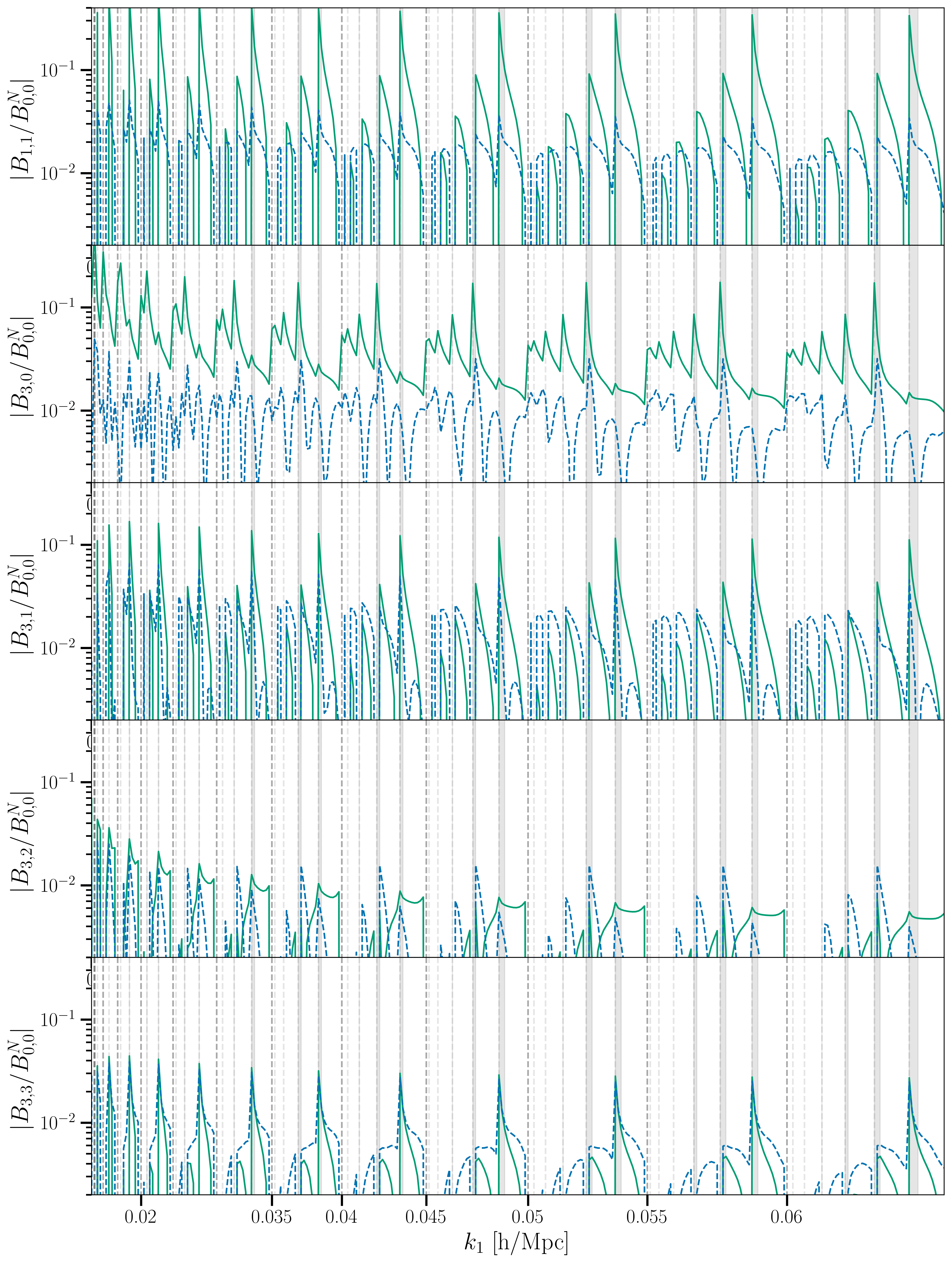
Figure 17: Relativistic (green) and wide-separation (blue) corrections to a selection of odd multipoles.

Appendix D Newtonian Local type Non-Gaussianity

We consider the local non-Gaussianity contribution, including scale-dependent biases, following [77], the non-Gaussian contributions to the first-order and second-order perturbations theory kernels are given by

$$Z^{(1)}_{\rm N,NG}=D(x_{1})b_{01}(x_{1})$$ (D.1)

and

$$Z^{(2)}_{\rm N,NG}=\,D^{2}(x_{1}) \left[b_{1}(x_{1})\left(f_{\rm NL}\frac{\alpha(q_{3})}{\alpha(q_{1})\alpha(q_{2})}\right)+f(x_{1})\frac{(\bm{q}_{12}\cdot\hat{\bm{x}}_{1})^{2}}{q^{2}_{12}}\left(f_{\rm NL}\frac{\alpha(q_{3})}{\alpha(q_{1})\alpha(q_{2})}\right)\right.$$ (D.2)

$$\,\left.\frac{b_{11}(x_{1})}{2}\left(\frac{1}{\alpha(q_{1})}+\frac{1}{\alpha(q_{2})}\right)+b_{01}(x_{1})\left(\frac{(\bm{q}_{1}\cdot\bm{q}_{2})}{q_{1}^{2}\alpha(q_{2})}+\frac{(\bm{q}_{1}\cdot\bm{q}_{2})}{q_{2}^{2}\alpha(q_{1})}\right)\right.$$

$$\,\left.+\frac{b_{02}(x_{1})}{\alpha(q_{1})\alpha(q_{2})}+\frac{b_{01}(x_{1})}{2}f(x_{1})(\bm{q}_{1}\cdot\hat{\bm{x}}_{1})\left(\frac{(\bm{q}_{1}\cdot\hat{\bm{x}}_{1})}{q_{1}^{2}\alpha(q_{2})}+\frac{(\bm{q}_{2}\cdot\hat{\bm{x}}_{1})}{q_{2}^{2}\alpha(q_{1})}\right)\right].$$

For models of the scale dependent biases, we follow the expressions in [77] and write the Eulerian expressions (we drop the explicit dependence on comoving distance)

$$b_{01} =b^{L}_{01},$$ (D.3a)

$$b_{11} =b^{L}_{01}+b^{L}_{11},$$ (D.3b)

$$b_{02} =b^{L}_{02},$$ (D.3c)

in terms of Lagrangian biases which, if one assumes a universal mass function, are given by

$$b_{01} =2\,\delta_{c}\,f_{\rm NL}\,b^{L}_{10},$$ (D.4a)

$$b_{11} =2\,f_{\rm NL}(\delta_{c}\,b^{L}_{20}-b^{L}_{10}),$$ (D.4b)

$$b_{02} =4\,f_{\rm NL}^{2}(\delta_{c}\,b^{L}_{20}-2\,b^{L}_{10}).$$ (D.4c)

Above, $\delta_{c}=1.686$ is the critical density for spherical collapse in an Einstein-de Sitter universe. The Lagrangian bias parameters in Equation (D.4) can then be expressed in terms of the Eulerian bias as

$$b^{L}_{10} =b_{10}-1,$$ (D.5a)

$$b^{L}_{20} =b_{20}-(8/21)\,b^{L}_{10}.$$ (D.5b)

The full redshift space kernels, at each order in perturbation theory, are>

$$Z^{(1)}=Z^{(1)}_{\rm G}+Z^{(1)}_{\rm N,NG},$$ (D.6)

and

$$Z^{(2)}=Z^{(2)}_{\rm G}+Z^{(2)}_{\rm N,NG},$$ (D.7)

and so the total primordial non-Gaussian contribution to the bispectrum can be calculated through Equation (2.22).

References

- [1] R. Scoccimarro, H.A. Feldman, J.N. Fry and J.A. Frieman, The bispectrum of IRAS redshift catalogs, The Astrophysical Journal 546 (2001) 652–664.
- [2] H.A. Feldman, J.A. Frieman, J.N. Fry and R. Scoccimarro, Constraints on galaxy bias, matter density, and primordial non-Gaussianity from the PSCz galaxy redshift survey, Physical Review Letters 86 (2001) 1434–1437.
- [3] A.F. Heavens, Estimating non-Gaussianity in the microwave background, Monthly Notices of the Royal Astronomical Society 299 (1998) 805–808.
- [4] P. Collaboration, Y. Akrami, F. Arroja, M. Ashdown, J. Aumont, C. Baccigalupi et al., Planck 2018 results. IX. Constraints on primordial non-Gaussianity, 2019.
- [5] D.J. Schlegel, S. Ferraro, G. Aldering, C. Baltay, S. BenZvi, R. Besuner et al., A spectroscopic road map for cosmic frontier: DESI, DESI-II, Stage-5, 2022.
- [6] A. Aghamousa, J. Aguilar, S. Ahlen, S. Alam, L.E. Allen, C.A. Prieto et al., The DESI experiment part I: science, targeting, and survey design, arXiv preprint arXiv:1611.00036 (2016) .
- [7] R. Laureijs, J. Amiaux, S. Arduini, J.L. Auguères, J. Brinchmann, R. Cole et al., Euclid definition study report, 2011.
- [8] O. Doré, J. Bock, M. Ashby, P. Capak, A. Cooray, R. de Putter et al., Cosmology with the SPHEREX All-Sky Spectral Survey, arXiv e-prints (2014) arXiv:1412.4872 [1412.4872].
- [9] D. Spergel, N. Gehrels, C. Baltay, D. Bennett, J. Breckinridge, M. Donahue et al., Wide-Field InfrarRed Survey Telescope-Astrophysics Focused Telescope Assets WFIRST-AFTA 2015 Report, 2015.
- [10] N. Sailer, E. Castorina, S. Ferraro and M. White, Cosmology at high redshift — a probe of fundamental physics, Journal of Cosmology and Astroparticle Physics 2021 (2021) 049.
- [11] F. Beutler and E. Di Dio, Modeling relativistic contributions to the halo power spectrum dipole, Journal of Cosmology and Astroparticle Physics 2020 (2020) 048.
- [12] D.J. Bacon, R.A. Battye, P. Bull, S. Camera, P.G. Ferreira, I. Harrison et al., Cosmology with phase 1 of the square kilometre array red book 2018: Technical specifications and performance forecasts, Publications of the Astronomical Society of Australia 37 (2020) .
- [13] P. Bull, Extending Cosmological Tests of General Relativity with the Square Kilometre Array, The Astrophysical Journal 817 (2016) 26.
- [14] C. Bonvin and R. Durrer, What galaxy surveys really measure, 1105.5280.
- [15] N. Kaiser, Clustering in real space and in redshift space, Monthly Notices of the Royal Astronomical Society 227 (1987) 1.
- [16] J. Yoo, A.L. Fitzpatrick and M. Zaldarriaga, New perspective on galaxy clustering as a cosmological probe: General relativistic effects, Physical Review D 80 (2009) .
- [17] J. Yoo and U. Seljak, Wide-angle effects in future galaxy surveys, Monthly Notices of the Royal Astronomical Society 447 (2015) 1789.
- [18] R. Scoccimarro, H.M.P. Couchman and J.A. Frieman, The bispectrum as a signature of gravitational instability in redshift space, The Astrophysical Journal 517 (1999) 531.
- [19] H. Gil-Marín, C. Wagner, J. Norena, L. Verde and W. Percival, Dark matter and halo bispectrum in redshift space: theory and applications, Journal of Cosmology and Astroparticle Physics 2014 (2014) 029.
- [20] C. Hahn, F. Villaescusa-Navarro, E. Castorina and R. Scoccimarro, Constraining M with the bispectrum. Part I. Breaking parameter degeneracies, Journal of Cosmology and Astroparticle Physics 2020 (2020) 040.
- [21] C. Clarkson, E.M. de Weerd, S. Jolicoeur, R. Maartens and O. Umeh, The dipole of the galaxy bispectrum, 1812.09512v3.
- [22] E.M. de Weerd, C. Clarkson, S. Jolicoeur, R. Maartens and O. Umeh, Multipoles of the relativistic galaxy bispectrum, 1912.11016v3.
- [23] D. Jeong and F. Schmidt, Parity-odd galaxy bispectrum, Physical Review D 102 (2020) 023530.
- [24] R. Scoccimarro, Fast estimators for redshift-space clustering, 1506.02729v2.
- [25] A.S. Szalay, T. Matsubara and S.D. Landy, Redshift-space distortions of the correlation function in wide-angle galaxy surveys, The Astrophysical Journal 498 (1998) L1.
- [26] T. Matsubara, The correlation function in redshift space: General formula with wide-angle effects and cosmological distortions, The Astrophysical Journal 535 (2000) 1.
- [27] I. Szapudi, Wide-angle redshift distortions revisited, The Astrophysical Journal 614 (2004) 51.
- [28] P. Pápai and I. Szapudi, Non-perturbative effects of geometry in wide-angle redshift distortions, Monthly Notices of the Royal Astronomical Society 389 (2008) 292.
- [29] D. Bertacca, R. Maartens, A. Raccanelli and C. Clarkson, Beyond the plane-parallel and newtonian approach: Wide-angle redshift distortions and convergence in general relativity, Journal of Cosmology and Astroparticle Physics 2012 (2012) 025.
- [30] F. Montanari and R. Durrer, New method for the Alcock-Paczyński test, Physical Review D 86 (2012) 063503.
- [31] P. Reimberg, F. Bernardeau and C. Pitrou, Redshift-space distortions with wide angular separations, Journal of Cosmology and Astroparticle Physics 2016 (2016) 048.
- [32] E. Castorina and M. White, Beyond the plane-parallel approximation for redshift surveys, Monthly Notices of the Royal Astronomical Society 476 (2018) 4403.
- [33] F. Beutler, E. Castorina and P. Zhang, Interpreting measurements of the anisotropic galaxy power spectrum, Journal of Cosmology and Astroparticle Physics 2019 (2019) 040.
- [34] P. Paul, C. Clarkson and R. Maartens, Wide-angle effects in multi-tracer power spectra with doppler corrections, 2208.04819v2.
- [35] S. Jolicoeur, S.L. Guedezounme, R. Maartens, P. Paul, C. Clarkson and S. Camera, Relativistic and wide-angle corrections to galaxy power spectra, arXiv e-prints (2024) arXiv:2406.06274 [2406.06274].
- [36] D. Bertacca, A. Raccanelli, N. Bartolo, M. Liguori, S. Matarrese and L. Verde, Relativistic wide-angle galaxy bispectrum on the light cone, Physical Review D 97 (2018) 023531.
- [37] C. Bonvin, L. Hui and E. Gaztañaga, Asymmetric galaxy correlation functions, Physical Review D 89 (2014) .
- [38] M. Noorikuhani and R. Scoccimarro, Wide-angle and relativistic effects in fourier-space clustering statistics, 2207.12383v1.
- [39] K. Pardede, E. Di Dio and E. Castorina, Wide-angle effects in the galaxy bispectrum, arXiv e-prints (2023) arXiv:2302.12789 [2302.12789].
- [40] E. Komatsu and D.N. Spergel, Acoustic signatures in the primary microwave background bispectrum, Physical Review D 63 (2001) 063002.
- [41] N. Dalal, O. Doré, D. Huterer and A. Shirokov, Imprints of primordial non-Gaussianities on large-scale structure: Scale-dependent bias and abundance of virialized objects, Phys. Rev. D 77 (2008) 123514.
- [42] S. Zaroubi and Y. Hoffman, Clustering in redshift space: Linear theory, astro-ph/9311013v2.
- [43] A. Hamilton, Linear redshift distortions: A review, The Evolving Universe: Selected Topics on Large-Scale Structure and on the Properties of Galaxies (1998) 185.
- [44] N.S. Sugiyama, S. Saito, F. Beutler and H.-J. Seo, A complete fft-based decomposition formalism for the redshift-space bispectrum, 1803.02132v3.
- [45] J. Byun and E. Krause, Modal compression of the redshift-space galaxy bispectrum, 2205.04579.
- [46] F. Bernardeau, S. Colombi, E. Gaztanaga and R. Scoccimarro, Large-scale structure of the universe and cosmological perturbation theory, astro-ph/0112551v1.
- [47] T. Matsubara, On Second-Order Perturbation Theories of Gravitational Instability in Friedmann-Lemaître Models, Progress of Theoretical Physics 94 (1995) 1151 [astro-ph/9510137].
- [48] T. Tram, C. Fidler, R. Crittenden, K. Koyama, G.W. Pettinari and D. Wands, The intrinsic matter bispectrum in cdm, Journal of Cosmology and Astroparticle Physics 2016 (2016) 058–058.
- [49] L. Verde, A.F. Heavens, S. Matarrese and L. Moscardini, Large-scale bias in the universe - ii. redshift-space bispectrum, Monthly Notices of the Royal Astronomical Society 300 (1998) 747–756.
- [50] J. Yoo, General relativistic description of the observed galaxy power spectrum: Do we understand what we measure?, 1009.3021.
- [51] A. Challinor and A. Lewis, Linear power spectrum of observed source number counts, 1105.5292.
- [52] D. Bertacca, R. Maartens and C. Clarkson, Observed galaxy number counts on the lightcone up to second order: I. Main result, 1405.4403.
- [53] D. Bertacca, R. Maartens and C. Clarkson, Observed galaxy number counts on the lightcone up to second order: II. Derivation, 1406.0319.
- [54] D. Bertacca, Observed galaxy number counts on the light cone up to second order: III. Magnification bias, Classical and Quantum Gravity 32 (2015) 195011 [1409.2024].
- [55] E. Di Dio, R. Durrer, G. Marozzi and F. Montanari, Galaxy number counts to second order and their bispectrum, 1407.0376.
- [56] J. Yoo and M. Zaldarriaga, Beyond the linear-order relativistic effect in galaxy clustering: Second-order gauge-invariant formalism, 1406.4140.
- [57] J.L. Fuentes, J.C. Hidalgo and K.A. Malik, Galaxy number counts at second order: an independent approach, Classical and Quantum Gravity 38 (2021) 065014.
- [58] O. Umeh, S. Jolicoeur, R. Maartens and C. Clarkson, A general relativistic signature in the galaxy bispectrum: the local effects of observing on the lightcone, 1610.03351.
- [59] S. Jolicoeur, O. Umeh, R. Maartens and C. Clarkson, Imprints of local lightcone \projection effects on the galaxy bispectrum. Part II, 1703.09630.
- [60] S. Jolicoeur, O. Umeh, R. Maartens and C. Clarkson, Imprints of local lightcone projection effects on the galaxy bispectrum. Part III. Relativistic corrections from nonlinear dynamical evolution on large-scales, 1711.01812.
- [61] C. Clarkson, E.M. de Weerd, S. Jolicoeur, R. Maartens and O. Umeh, The dipole of the galaxy bispectrum, Monthly Notices of the Royal Astronomical Society: Letters 486 (2019) L101–L104.
- [62] J.N. Benabou, I. Sands, H.S.G. Gebhardt, C. Heinrich and O. Doré, Wide-angle effects in the power spectrum multipoles in next-generation redshift surveys, 2024.
- [63] K. Pardede, F. Rizzo, M. Biagetti, E. Castorina, E. Sefusatti and P. Monaco, Bispectrum-window convolution via Hankel transform, 2203.04174.
- [64] Square Kilometre Array Cosmology Science Working Group, D.J. Bacon, R.A. Battye, P. Bull, S. Camera, P.G. Ferreira et al., Cosmology with Phase 1 of the Square Kilometre Array Red Book 2018: Technical specifications and performance forecasts, 1811.02743.
- [65] Planck Collaboration, N. Aghanim, Y. Akrami, M. Ashdown, J. Aumont, C. Baccigalupi et al., Planck 2018 results. VI. Cosmological parameters, 1807.06209.
- [66] R. Maartens, J. Fonseca, S. Camera, S. Jolicoeur, J.-A. Viljoen and C. Clarkson, Magnification and evolution biases in large-scale structure surveys, 2107.13401.
- [67] R. Maartens, S. Jolicoeur, O. Umeh, E.M. De Weerd, C. Clarkson and S. Camera, Detecting the relativistic galaxy bispectrum, 1911.02398.
- [68] S. Yahya, P. Bull, M.G. Santos, M. Silva, R. Maartens, P. Okouma et al., Cosmological performance of SKA H I galaxy surveys, 1412.4700.
- [69] T. Lazeyras, C. Wagner, T. Baldauf and F. Schmidt, Precision measurement of the local bias of dark matter halos, 1511.01096.
- [70] D.J. Schlegel, J.A. Kollmeier, G. Aldering, S. Bailey, C. Baltay, C. Bebek et al., The MegaMapper: A Stage-5 Spectroscopic Instrument Concept for the Study of Inflation and Dark Energy, arXiv e-prints (2022) arXiv:2209.04322 [2209.04322].
- [71] A. Barreira, The squeezed matter bispectrum covariance with responses, 1901.01243.
- [72] M. Biagetti, L. Castiblanco, J. Noreña and E. Sefusatti, The covariance of squeezed bispectrum configurations, 2111.05887.
- [73] J. Salvalaggio, L. Castiblanco, J. Noreña, E. Sefusatti and P. Monaco, Bispectrum non-Gaussian Covariance in Redshift Space, 2403.08634.
- [74] D. Karagiannis, R. Maartens, J. Fonseca, S. Camera and C. Clarkson, Multi-tracer power spectra and bispectra: formalism, 2305.04028.
- [75] O. Umeh, S. Jolicoeur, R. Maartens and C. Clarkson, A general relativistic signature in the galaxy bispectrum: the local effects of observing on the lightcone, 1610.03351.
- [76] E. Di Dio, H. Perrier, R. Durrer, G. Marozzi, A. Moradinezhad Dizgah, J. Noreña et al., Non-Gaussianities due to relativistic corrections to the observed galaxy bispectrum, 1611.03720.
- [77] M. Tellarini, A.J. Ross, G. Tasinato and D. Wands, Galaxy bispectrum, primordial non-Gaussianity and redshift space distortions, Journal of Cosmology and Astroparticle Physics 2016 (2016) 014.
- [78] R. Maartens, S. Jolicoeur, O. Umeh, E.M. De Weerd and C. Clarkson, Local primordial non-Gaussianity in the relativistic galaxy bispectrum, 2011.13660.
- [79] G. D’Amico, M. Lewandowski, L. Senatore and P. Zhang, Limits on primordial non-Gaussianities from BOSS galaxy-clustering data, arXiv e-prints (2022) arXiv:2201.11518 [2201.11518].
- [80] J. Lesgourgues, The Cosmic Linear Anisotropy Solving System (CLASS) I: Overview, arXiv e-prints (2011) arXiv:1104.2932 [1104.2932].
- [81] D. Blas, J. Lesgourgues and T. Tram, The cosmic linear anisotropy solving system (class). part ii: Approximation schemes, Journal of Cosmology and Astroparticle Physics 2011 (2011) 034–034.
- [82] C.R. Harris, K.J. Millman, S.J. van der Walt, R. Gommers, P. Virtanen, D. Cournapeau et al., Array programming with NumPy, Nature 585 (2020) 357.
- [83] P. Virtanen, R. Gommers, T.E. Oliphant, M. Haberland, T. Reddy, D. Cournapeau et al., SciPy 1.0: Fundamental Algorithms for Scientific Computing in Python, Nature Methods 17 (2020) 261.
- [84] J.D. Hunter, Matplotlib: A 2d graphics environment, Computing in Science & Engineering 9 (2007) 90.
- [85] K.C. Chan and L. Blot, Assessment of the information content of the power spectrum and bispectrum, 1610.06585.