Adaptive and Parallel Multiscale Framework for Modeling Cohesive Failure in Engineering Scale Systems

Abstract

The high computational demands of multiscale modeling necessitate advanced parallel and adaptive strategies. To address this challenge, we introduce an adaptive method that utilizes two microscale models based on an offline database for multiscale modeling of curved interfaces (e.g., adhesive layers). This database employs nonlinear classifiers, developed using Support Vector Machines from microscale sampling data, as a preprocessing step for multiscale simulations. Next, we develop a new parallel network library that enables seamless model selection with customized communication layers, ensuring scalability in parallel computing environments. The correctness and effectiveness of the hierarchically parallel solver are verified on a crack propagation problem within the curved adhesive layer. Finally, we predict the ultimate bending moment and adhesive layer failure of a wind turbine blade and validate the solver on a difficult large-scale engineering problem.

1 Introduction

The rapid expansion of composite materials in aerospace, wind energy, automotive, and other industries has stimulated significant research interest in multiscale methods. In general, multiscale methods have the ability to construct the constitutive response from data at lower scales and can efficiently transform epistemic uncertainty (i.e., reducible uncertainty) in the parameters of coarse-grained models into the aleatoric uncertainty (i.e., irreducible uncertainty) of finer-grained models. Review articles by Matouš et al. [45], Fish et al. [23], Schlick et al. [65], and Geers et al. [26] highlight important milestones in multiscale modeling and delineate outstanding challenges.

Multiscale methods, and homogenization in particular, trace back to micromechanics. Early models, such as those by Sachs [62], Taylor [69], Eshelby [18], Willis [76], and Hill [32], among others, were developed to estimate effective macroscopic constitutive equations. The “homogenization” method was originally conceived by Ivo Babuška [1] and many following works provided rigor to its foundation (see the work of Benssousan et al. [5], and Sanchez-Palencia [64], for example).

Since its early development, many powerful homogenization methods have been developed for a variety of engineering problems, with work by Fish [22], Geers et al. [27], Ghosh et al., [28], Khisaeva and Ostoja-Starzewski [35], Temizer and Zohdi [70], Terada et al. [71], Miehe et al. [49], Ponte Castañeda [11], Michel et al. [47], Feyel and Chaboche [21], Matouš et al. [46], and many other scholars. Today, homogenization is regarded as a well-developed discipline with an impact on industry and academia alike.

Figure 1: National Rotor Testbed 13 m wind turbine blade. (from Murray et al. [54])

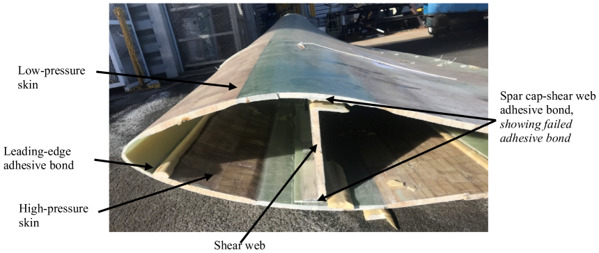
In this article, we are particularly interested in the multiscale modeling of adhesive layers. Adhesive layers are critical in many engineering applications. Fig. 1 shows progressive debonding of a 13 m wind turbine blade designed by Sandia National Laboratories [34] and structurally tested at the National Wind Technology Center [25]. During the ultimate static test, the adhesive joint failed between the shear web and the spar cap on the low-pressure side. This highlights the modeling challenges of capturing the structural response of the blade as well as the highly nonlinear response of the adhesive. To address the modeling challenges of adhesive failure, Matouš et al. [46, 38, 37] developed a multiscale scheme for interfaces, which was later expanded to finite strains [33, 52]. The first three-dimensional (3D) hierarchically parallel implementation was developed by Mosby and Matouš [51, 53] and successfully applied to large multiscale problems.

Unfortunately, the computational complexity of multiscale modeling remains a bottleneck, and many researchers have focused on developing Reduced-Order Models (ROM). Oskay and Fish [58] developed eigendeformation-based reduced order homogenization. Yvonnet and He developed a reduced model multiscale method [77]. Michel and Suquet developed a nonuniform transformation field analysis [48]. van Tuijl et al. [72] developed a wavelet based reduced order model. Bhattacharjee and Matouš [6, 7] developed a manifold-based reduced order model. Le et al. [39] used neural networks for computational homogenization. Beel and Fish proposed solver-free reduced order homogenization [4]. Adaptive multiscale modeling is also popular [19, 29, 9, 13, 3, 57, 56, 73]. Furthermore, we highlight the impact of machine learning on multiscale modeling [59, 74, 12, 8, 42].

In this work, we develop a novel adaptive and parallel multiscale framework that combines both model reduction and efficient parallel implementation. In particular, we focus on Computational Homogenization (CH) and microscale model selection [2], which are crucial for solving real industrially relevant problems, like in Fig. 1. For large engineering problems, multiscale simulations are usually needed in only a small portion of the computational domain (i.e., the damage-prone regions of the adhesive layer), and the rest of the structure can be modeled using a ROM or a phenomenological constitutive model. However, the matter of how to effectively select from a list of models is a nontrivial task, especially in a parallel multiscale environment where each model requires different computational resources. To address this issue, we rely on Support Vector Machines (SVMs) [14, 17], which are supervised max-margin models with associated learning algorithms that analyze data for regression analysis and classification. SVMs offer potential for enhancing statistical analysis in multiscale modeling due to their robust mathematical foundations and scalability [44, 31, 67]. We extend the 3D multiscale modeling of interfaces [51] to problems with curvature, which requires a careful computational treatment of the unit cell normal. Moreover, we develop a novel multiscale network library that allows uninterrupted dynamic microscale model selection and computer resource allocation in a parallel setting. We verify the framework on the Double-Cantilever Beam (DCB) with a curved interface and validate it on a difficult National Rotor Testbed (NRT) engineering problem.

The remainder of this paper is organized as follows. In Section 2, we overview the governing equations for CH and SVMs. Section 3 explores the adaptive strategy for selecting microscale models. In Section 4, we introduce the supporting network for parallel and adaptive multiscale simulation. Following this, Section 5 discusses the constitutive model alongside the numerical implementation. Section 6 presents numerical examples. Finally, the conclusions are drawn in Section 7.

2 Governing equations

In this section, we present computational homogenization for interfaces and SVMs for model selection. Building upon the previous multiscale work outlined in [53], we develop and incorporate a novel adaptive strategy suitable for high-performance computing (i.e, parallel computing). The following subsections will cover both macro and micro scale problems, with an overview of Support Vector Regression (SVR), which is a variant of the SVM, as the methodology for microscale model adaption.

2.1 Computational homogenization for interfaces

For clarity of presentation, we revisit multiscale cohesive modeling in a finite strain setting as originally developed in [46, 51, 52]. The position of a macroscopic material point is defined as $\vec{X}\in\Omega_{0}$ in a body $\Omega_{0}\subset\mathbb{R}^{3}$, and the position of a microscopic material point is defined as $\vec{Y}\in\Theta_{0}$ in a microstructure $\Theta_{0}\subset\mathbb{R}^{3}$, as shown in Fig. 2. The adhesive layer is represented by the domain $\Gamma_{0}\subset\mathbb{R}^{2}$ with a positive thickness $l_{c}$ linking two adherends $\Omega_{0}^{\pm}$ and a normal to the interface ${}^{0}\vec{N}$. The boundary is decomposed into $\partial\Omega^{u}_{0}$ and $\partial\Omega^{\text{t}}_{0}$, for the applied displacement $\hat{\vec{u}}$ and traction $\hat{\vec{t}}$ vectors respectively, satisfying the relations $\partial\Omega_{0}=\partial\Omega_{0}^{u}\cup\partial\Omega_{0}^{\text{t}}$ and $\partial\Omega_{0}^{u}\cap\partial\Omega_{0}^{\text{t}}=\emptyset$.

Figure 2: Kinematics of multiscale cohesive modeling in a finite strain setting. $\Omega_{0}^{\pm}$ are the macroscale domains, while $\Theta_{0}$ represents the microscale domain.

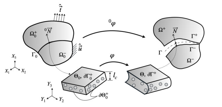
Within the multiscale cohesive modeling framework, the average deformation gradient on the interface $\Gamma_{0}$ is defined by the jump across the layer $\llbracket{}^{0}\varphi\,\rrbracket={}^{0}\varphi^{+}-{}^{0}\varphi^{-}=\llbracket{}^{0}\vec{u}\,\rrbracket$. Thus, the macroscale deformation gradients read ${}^{0}\boldsymbol{F}=\nabla_{\vec{X}}{}^{0}\varphi=\boldsymbol{1}+\nabla_{\vec{X}}{}^{0}\vec{u}$ for the macroscale domain $\Omega_{0}^{\pm}$, and ${}^{0}\boldsymbol{F}=\boldsymbol{1}+\nicefrac{{1}}{{l_{c}}}\llbracket{}^{0}\vec{u}\,\rrbracket\otimes{}^{0}\vec{N}$ for the interface $\Gamma_{0}$. The macroscale boundary value problem stems from the linear momentum balance. By neglecting inertial terms and body forces, we obtain

$$\nabla_{\vec{X}}\cdot({}^{0}\boldsymbol{F}\,{}^{0}\boldsymbol{S})=\vec{0}\quad \in\Omega_{0},$$ (1)

$${}^{0}\boldsymbol{P}\cdot{}^{0}\vec{N}=\hat{\vec{t}}\quad \text{on }\partial\Omega_{0}^{\text{t}},$$ (2)

$${}^{0}\vec{u}=\hat{\vec{u}}\quad \text{on }\partial\Omega_{0}^{u},$$ (3)

$${}^{0}\vec{t}^{+}+{}^{0}\vec{t}^{-}=\vec{0}\quad \in\Gamma_{0},$$ (4)

where ${}^{0}\boldsymbol{P}={}^{0}\boldsymbol{F}\,{}^{0}\boldsymbol{S}$ and ${}^{0}\boldsymbol{S}=2\partial\,{}^{0}W({}^{0}\boldsymbol{C})/\partial\,{}^{0}\boldsymbol{C}$ are the first (PK1) and the second Piola-Kirchhoff (PK2) stress tensors, respectively. Here, PK2 is derived from the macroscale strain energy density function ${}^{0}W({}^{0}\boldsymbol{C})$ and ${}^{0}\boldsymbol{C}={}^{0}\boldsymbol{F}^{\top}\,{}^{0}\boldsymbol{F}$ denotes the macroscopic right Cauchy–Green deformation tensor.

The microscale deformation gradient is represented as $\boldsymbol{F}={}^{0}\boldsymbol{F}+\nabla_{\vec{Y}}{}^{1}\vec{u}$. By neglecting the body forces and assuming no prescribed traction, we obtain the microscale boundary value problem

$$\nabla_{\vec{Y}}\cdot(\boldsymbol{F}\,{}^{1}\boldsymbol{S})=\vec{0}\quad \forall\,\vec{Y}\in\Theta_{0},$$ (5)

$$\varphi=\hat{\varphi}\quad \text{on }\partial\Theta_{0},$$ (6)

where ${}^{1}\boldsymbol{S}=2\partial{}^{1}W(\boldsymbol{C})/\partial\boldsymbol{C}$ is the microscale PK2 stress tensor, ${}^{1}W(\boldsymbol{C})$ represents the microscale strain energy density function, and $\boldsymbol{C}=\boldsymbol{F}^{\top}\boldsymbol{F}$ is the microscale right Cauchy-Green deformation tensor.

We bridge the macroscale and microscale boundary value problems through the Hill-Mandel energy equivalence [32]

$$\inf_{\llbracket{}^{0}\vec{u}\,\rrbracket}{}^{0}W(\llbracket{}^{0}\vec{u}\,\rrbracket)=\inf_{\llbracket{}^{0}\vec{u}\,\rrbracket}\inf_{{}^{1}\vec{u}}\frac{l_{c}}{|\Theta_{0}|}\int_{\Theta_{0}}{}^{1}W({}^{0}\boldsymbol{F}+\nabla_{\vec{Y}}{}^{1}\vec{u})\,\text{d}\Theta_{0},$$ (7)

which is usually formulated for dissipative processes in terms of work conjugated pairs [27, 45]. The micro-to-macro transition for the cohesive traction vector ${}^{0}\vec{t}$ is given by

$${}^{0}\vec{t}=\frac{1}{|\Theta_{0}|}\bigg{[}\int_{\Theta_{0}}\boldsymbol{F}\,{}^{1}\boldsymbol{S}\,\text{d}\Theta_{0}\bigg{]}\cdot{}^{0}\vec{N}.$$ (8)

As presented for interfaces in the work of Matouš et al. [46], we can use two sets of microscale boundary conditions

$${}^{1}\vec{u}=\vec{0}\,\,\text{on }\partial\Gamma_{0}^{\pm},\quad{}^{1}\vec{u}^{+}-{}^{1}\vec{u}^{-} =\vec{0}\,\,\text{on }\partial\Theta_{0}^{\pm},\quad{}^{1}\vec{t}^{+}+{}^{1}\vec{t}^{-}=\vec{0}\,\,\text{on }\partial\Theta_{0}^{\pm},$$ (9)

$${}^{1}\vec{u} =\vec{0}\quad\forall\,\vec{Y}\in\Theta_{0},$$ (10)

which allows us to introduce a seamless model adaption at the microscale. The typical semi-periodic boundary conditions, as given by Eq. (9), involve solving the microscale BVP of Eq. (5) using a numerical method (e.g., finite element method). This leads to high accuracy, but the computational cost is unfortunately high. We will refer to this approach as the Full Model (FM). Conversely, Eq. (10) describes the Taylor Model (TM) which neglects fluctuations within $\Theta_{0}$, leading to a relatively low computational cost in solving Eq. (5) due to its linear structure (i.e., summation). On the other hand, the accuracy of TM is lower than FM.

2.2 Interface normal

When dealing with adhesives that have complex geometries, it becomes necessary to define the normal to the interface, ${}^{0}\vec{N}$ (see Fig. 2). The macroscale normal vector ${}^{0}\vec{N}$ needs to be perpendicular to the unit cell top boundary. In this work, the rotation matrix is calculated using the outer product, considering that the macroscale and microscale coordinates share only one common basis vector, $\vec{X}_{1}=\vec{Y}_{1}$, at a material point $\vec{x}\in\Gamma_{0}$. We can make this connection between the macroscale and microscale basis vectors as we focus on statistically isotropic particulate systems. The rotation matrix $\boldsymbol{R}$ is given by

$$\boldsymbol{R}=\left(\begin{array}[]{c}\vec{Y}^{*}_{1}\\ {}^{0}\vec{N}\times{\vec{Y}}^{*}_{1}\\ {}^{0}\vec{N}\\ \end{array}\right),$$ (11)

where $\vec{Y}^{*}=\boldsymbol{R}\vec{Y}$ is the new microscale point and $\boldsymbol{R}^{\top}\boldsymbol{R}=\boldsymbol{1}$. In a discrete setting, we minimize the difference between $\vec{X}_{1}$ and $\vec{Y}^{*}_{1}$ by projecting

$$\vec{Y}^{*}_{1}=\vec{X}_{1}-\frac{\vec{X}_{1}\cdot{}^{0}\vec{N}}{||{}^{0}\vec{N}||}{}^{0}\vec{N},$$ (12)

to eliminate possible drift due to the finite element discretization.

2.3 Support vector regression for microscale model selection

Selecting the appropriate microscale model on the fly, whether FM or TM, is challenging when solving the coupled multiscale problem. The interface, $\Gamma_{0}$, contains a large number of cohesive elements and it is important to select FM or TM appropriately to retain the required accuracy with minimal computational cost. Specifically, it is desirable to adopt FM over areas of interest with large deformation gradients and/or high stresses. On the other hand, TM can be used in regions that are smooth.

Consequently, this process of selection effectively turns into a statistical problem, characterized by assigning labels of $y=+1$ to FM and $y=-1$ to TM. In statistical classification problems with two classes, a decision boundary is built as a hypersurface that separates the underlying vector space into two sets, one for each class (i.e., FM or TM). Decision boundaries can be clear-cut when the classes are linearly separable, but they may be ambiguous in fuzzy logic-based classification algorithms. An SVM finds the hyperplane with the maximum margin [14], and the kernel trick is adopted to turn the nonlinearly separable problem into a linearly separable one.

First, we define a SVM data point (i.e., a sample) as a jump displacement $\vec{x}=\llbracket{}^{0}\vec{u}\rrbracket$ within the cohesive element on $\Gamma_{0}$. Next, to retain the loading magnitude $r=\|\llbracket{}^{0}\vec{u}\rrbracket\|$ over the Representative Unit Cell (RUC), we introduce the jump vector components in a spherical coordinate system

$$\llbracket{}^{0}u_{1}\rrbracket =r\cos\phi\sin\theta,$$ (13)

$$\llbracket{}^{0}u_{2}\rrbracket =r\sin\phi\sin\theta,$$ (14)

$$\llbracket{}^{0}u_{3}\rrbracket =r\cos\theta,$$ (15)

where $r$ is the radial distance, $\phi$ is the azimuthal angle, and $\theta$ is the polar angle. Thus, when the magnitude of $r$ is constant, the sampling space becomes 2D with $\vec{x}=\left(\phi,\theta\right)$.

To proceed, we consider $\varepsilon$-insensitive SVR [17] with the kernel trick for nonlinear cases. In the binary SVM problem, we are given a training dataset consisting of $N_{t}$ samples for each constant $r$ denoted as

$$\{(\vec{x}_{i},y_{i});\,i=1,2,\ldots,N_{t}\},$$ (16)

where each point is a two-dimensional real vector $\vec{x}_{i}\in\mathbb{R}^{2}$ with labels $y_{i}=\pm 1$ corresponding to FM and TM simulations respectively. To create a nonlinear classifier, we adopt one of the most commonly used Gaussian functions as a positive semi-definite kernel

$$k(\vec{x}_{i},\vec{x})=\exp{(-|\vec{x}_{i}-\vec{x}|^{2})/\sigma^{2}},$$ (17)

where the depth of the kernel is denoted as $\sigma>0$, and $\vec{x}$ is a new data point to be classified. By introducing a dual set of variables $\alpha_{i}$ and $\alpha_{i}^{*}$, the dual formula can be expressed with an error tolerance of $\varepsilon$ that leads to

$$\max_{\alpha_{i},\alpha_{i}^{*}}\,\,\,\, -\frac{1}{2}\sum_{i=1}^{N_{t}}\sum_{j=1}^{N_{t}}(\alpha_{i}-\alpha_{i}^{*})(\alpha_{j}-\alpha_{j}^{*})k(\vec{x}_{i},\vec{x}_{j})-\varepsilon\sum_{i=1}^{N_{t}}(\alpha_{i}+\alpha_{i}^{*})+\sum_{i=1}^{N_{t}}y_{i}(\alpha_{i}-\alpha_{i}^{*}),$$ (18)

subject to $$\quad\hskip 42.67912pt\sum_{i=1}^{N_{t}}(\alpha_{i}-\alpha_{i}^{*})=0,\,\,\,0\leq\alpha_{i}\leq C,\,\,\,0\leq\alpha_{i}^{*}\leq C,$$ (19)

where $C$ is a positive constant. The sample $\vec{x}_{i}$ becomes a Support Vector (SV) when $\alpha_{i}-\alpha_{i}^{*}\neq 0$. Note that the Karush-Kuhn-Tucker complementarity conditions exist to explain violation tolerance and the SV vectors can be evaluated [15, 24]. This quadratic programming problem is solved by a sequential minimal optimization algorithm [20]. Data training can be seen as the process of determining a regression function denoted by $f(\vec{x})$, often referred to as the score function. Ultimately, we obtain the nonlinear SVM score function for any newly added data points $\vec{x}$,

$$f(\vec{x})=\sum_{\vec{x}_{i}\in SV}^{N_{t}}(\alpha_{i}-\alpha_{i}^{*})k(\vec{x}_{i},\vec{x})+b,$$ (20)

where $b$ represents the bias.

3 Adaptive multiscale strategy

The fundamental concept of the adaptive multiscale strategy is to introduce an offline database through SVR training to accelerate multiscale simulations. Over the course of this training, we generate numerous samples to measure modeling errors. Subsequently, we label each sample as either FM or TM based on a user-defined error tolerance to build the decision boundary.

In detail, we train the nonlinear SVM classifiers utilizing RUCs under various loading conditions, $\vec{x}=(\phi,\theta)$. Following this, we set a range for the magnitude of $r$ introducing the maximum jump displacement $\lambda=\max(\|\llbracket{}^{0}\vec{u}\rrbracket\|)$,

$$0\leq r\leq\lambda.$$ (21)

We uniformly discretize the span into $N_{s}$ segments to limit the number of total training steps (i.e., $N_{s}\times N_{t}$). Therefore, we can represent a set of radial distances as $\left\{r_{1},r_{2},\cdots,r_{N_{s}}\right\}=\nicefrac{{\lambda}}{{N_{s}}}\left\{1,\,2,\,\cdots,\,N_{s}\right\}$. Each radial distance covers an equal-sized segment (e.g., $0\leq r_{1}\leq\nicefrac{{\lambda}}{{N_{s}}}$ and $\nicefrac{{\lambda}}{{N_{s}}}<r_{2}\leq\nicefrac{{2\lambda}}{{N_{s}}}$). Finally, we generate an $i$-th training sample for each radial distance, $\vec{x}_{i}=(\phi_{i},\theta_{i})$, satisfying

$$\phi_{i} =2\pi H^{i}_{1},$$ (22)

$$\theta_{i} =\pi H^{i}_{2},$$ (23)

where $H^{i}$ is the $i$-th member of 2D Halton sequence [30], with subscripts $(\bullet)_{1}$ and $(\bullet)_{2}$ for the first and second bases, respectively. In this work, this quasi-random sequence skips the first 1000 values and retains every 101st point followed by a reverse-radix scrambling algorithm [36]. This approach ensures that any dense clusters created by naive random sampling are removed and facilitates easier implementation of low-discrepancy sequences [75].

For each sample generated, we obtain a solution from Eq. (5) for two sets of microscale boundary conditions (i.e., FM and TM) in Eqs. (9) and (10). Then, we establish a metric to evaluate the modeling errors, each with subscripts $(\bullet)_{FM}$ and $(\bullet)_{TM}$ to denote FM and TM, respectively. In this work, the error metric is based on the traction vector

$$\mathcal{E}_{{}^{0}\vec{t}} =\frac{\|{}^{0}\vec{t}_{FM}-{}^{0}\vec{t}_{TM}\|}{\|{}^{0}\vec{t}_{FM}\|}.$$ (24)

By introducing a user-defined modeling tolerance $\gamma$, we choose the modeling error for each sample to ensure that $\mathcal{E}_{{}^{0}\vec{t}}<\gamma$ when labeling the training samples $\vec{x}_{i}$ with TM. Otherwise, we use FM. In the special case of unknown modeling error that violates Eq. (21), all training samples are considered FM. As a consequence of this labeling process, we assemble an offline database, $\mathcal{DB}$, as a collection of trained score functions with the nonlinear decision boundaries

$$\mathcal{DB}=\left\{f_{1}(\vec{x}),f_{2}(\vec{x}),\ldots,f_{N_{s}}(\vec{x})\right\}.$$ (25)

4 Adaptive and parallel multiscale network

Figure 3: Dependency trees of the adaptive multiscale network and parallel communication patterns.

In a highly parallel computational environment managing two microscale models emerges as the key challenge within the adaptive multiscale modeling. This complexity arises because each microscale model (i.e., $\mathcal{D}_{1}-$FM and $\mathcal{D}_{2}-$TM) demands an additional network abstraction layer in the dependency trees as shown in Fig. 3. Moreover, the dependency trees necessitate inter-object communications (shown by the dashed lines). The macroscopic computational domain $\mathcal{D}_{0}$ assigns one job for each cohesive element at the interface $\Gamma_{0}$ (see Fig. 2). The microscale model adaption (i.e., FM and TM), triggered by $\mathcal{D}_{0}$ jobs, leads to the dynamic evolution of computational domains $\mathcal{D}_{i}$. These domains are mapped to the microscale servers $\mathcal{S}_{i}$ requiring load balancing. Subsequently, virtual services (i.e., $\mathcal{D}_{i}$ mapping to $\mathcal{S}_{i}$ and load balancing) call for proper partitioning and management of computational resources.

Figure 4: Schematic of the workload balance through inter-domain communication for computational jobs. In this example, five jobs are processed by three servers between time steps $t_{n}$ and $t_{n+1}$.

In this work, we present a novel multiscale network library – multiscale_net – that allows for uninterrupted dynamic microscale model selection in a parallel setting. multiscale_net is written in object-oriented C$++$ using the Message Passing Interface (MPI). New communicators (COMM) are designed to manage the computational domains $\mathcal{D}_{i}$. To distinguish between the three computations (i.e., macroscale, FM and TM microscales), the generalized launch specification assigns each numerical object (i.e., macroscale, FM, and TM) to a corresponding domain (i.e., $\mathcal{D}_{0}-$M, $\mathcal{D}_{1}-$FM, and $\mathcal{D}_{2}-$TM). The macroscopic domain $\mathcal{D}_{0}$ is executed on a set of processors ($P_{1},\cdots,P_{M}$) where $P_{1}$ denotes the master processor, and $P_{2},\cdots,P_{M}$ are worker processor. In addition, $\mathcal{D}_{0}$ uses inter-domain communications to link the microscopic domains $\mathcal{D}_{i}$ to servers $\mathcal{S}_{i}$ resulting in mappings $\mathcal{D}_{1}(\mathcal{S}_{i})$ and $\mathcal{D}_{2}(\mathcal{S}_{i})$. Each of the macroscale processors (i.e., $P_{i}$ in $\mathcal{D}_{0}$) communicates with the master processor of each microscale server (i.e., $p_{1}$ in $\mathcal{S}_{i}$) with $p_{2},\cdots,p_{m}$ being worker processors. The typical master-worker relation is established through intra-group communications within each processor set (i.e., $\mathcal{S}_{i}$). Furthermore, due to the computational load imbalance between FM and TM, domains $\mathcal{D}_{i}$ are dynamically reassigned to microscale servers $\mathcal{S}_{j}$ based on the largest first algorithm [41]. To achieve this, the inter-group communication between microscale servers is restricted to processors sharing the same task IDs, which leads to $p_{i}$ in $S_{j}$ communicating with $p_{i}$ in $\mathcal{S}_{k}$, $\forall i=2,\cdots,m$. This simplifies RUC data migration on available microscale servers, and reduces the complexity of communication patterns. The procedure for balancing the workload between time steps $t_{n}$ and $t_{n+1}$ is summarized in Fig. 4.

5 Numerical implementation and constitutive models

The numerical implementation using FEM has been described in [51, 52]. The weak forms of the macroscale and microscale boundary value problems, Eq. (1) and Eq. (5), are derived from a standard variational procedure and we do not repeat them here for brevity. We implement SVM based adaption as well as $multiscale\_net$ into our in-house massively parallel library $PGFem3D$ for both single-scale and multiscale simulations. The $PGFem3D$ solver has been rigorously verified and validated in several previous studies [40, 51, 52, 53, 68]. For mesh generation, we employ $T3D$ meshing tool [60, 61] and create linear tetrahedral meshes for both single-scale and multiscale simulations. The remaining task involves specifying the constitutive models at the macroscale, Eq. (1), and at the microscale, Eq. (5).

At the macroscale, we use the typical Neo-Hookean solid

$${}^{0}W(\hat{{}^{0}\boldsymbol{C}}) =\frac{{}^{0}\mu}{2}[\text{tr}({}^{0}\hat{\boldsymbol{C}})-3],$$ (26)

$${}^{0}U({}^{0}J) =\frac{{}^{0}\kappa}{2}[\text{exp}({}^{0}J-1)-\text{ln}({}^{0}J)-1],$$ (27)

where ${}^{0}\hat{W}({}^{0}\boldsymbol{C})$ represents the deviatoric and ${}^{0}U({}^{0}J)$ the volumetric component of the macroscale strain energy density function. The macroscale Jacobian is defined as ${}^{0}J=\text{det}({}^{0}\boldsymbol{F})$. Also, ${}^{0}\mu$ denotes the macroscale shear modulus, ${}^{0}\kappa$ is the macroscale bulk modulus, and ${}^{0}\hat{\boldsymbol{C}}={}^{0}J^{-\nicefrac{{2}}{{3}}}\,{}^{0}\boldsymbol{C}$ represents the macroscale deviatoric right Cauchy-Green deformation tensor.

At the microscale, we use the continuum damage model developed by Lee et al. [40], which relies on the split of the strain energy density function and the damage variable

$${}^{1}W(\boldsymbol{C},\omega^{d},\omega^{v})=(1-\omega^{d}){}^{1}\hat{W}(\boldsymbol{C})+(1-\omega^{v}){}^{1}U(J),$$ (28)

where $\omega^{d}\in[0,1)$ and $\omega^{v}\in[0,1)$ are the deviatoric and volumetric damage variables, respectively. The total damage variable is defined by $\omega=\sqrt{(\omega^{d})^{2}+(\omega^{v})^{2}}/\sqrt{2}$. Similar to the macroscale, we use the typical Neo-Hookean strain energy density functions ${}^{1}W(\hat{\boldsymbol{C}})$ and ${}^{1}U(J)$ (see Eqs.(26) and (27)) along with the corresponding deformation tensor $\boldsymbol{C}$, Jacobian $J$, and microscale material parameters $\mu$ and $\kappa$.

The microscale PK2 stress is derived from the microscale strain energy densities as

$${}^{1}\boldsymbol{S}=(1-\omega^{d})2\frac{\partial{}^{1}\hat{W}}{\partial\boldsymbol{C}}+(1-\omega^{v})\frac{\partial{}^{1}U}{\partial J}J\boldsymbol{C}^{-1}.$$ (29)

The split damage model is energy-driven and the evolution equations for $\dot{\omega}^{d}$ and $\dot{\omega}^{v}$ are derived from the damage energy release rates given by

$$Y^{\bullet}({}^{1}\hat{W},{}^{1}U)=\alpha^{\bullet}\,{}^{1}\hat{W}+\beta^{\bullet}\,{}^{1}U,$$ (30)

where $()^{\bullet}$ denotes either the deviatoric $()^{d}$ or the volumetric $()^{v}$ contribution. $\alpha^{d},\alpha^{v}\in[0,1]$ and $\beta^{d},\beta^{v}\in[0,1]$ are material parameters controlling the degree of volumetric and deviatoric coupling. We use $\alpha^{d}=\alpha^{v}=1\;\forall J$, $\beta^{d}=\beta^{v}=1\;\forall J\geq 1$ and $\beta^{d}=\beta^{v}=0\;\forall J<1$, to prevent pure volumetric damage under compression. More details are provided in Lee et al. [40].

6 Numerical examples

In this section, we present two numerical studies using our novel adaptive multiscale strategy. The first verification study is designed to assess the functionality of our adaptive approach. In this example, we demonstrate progressive failure using a DCB with a curved interface. Next, we simulate a large and industrially relevant wind turbine blade application. In particular, we use the National Rotor Testbed [25] that reports on the failure of a 13 meter-long wind turbine blade under ultimate static test.

6.1 Double-cantilever beam

At the macroscale, two adherends are bonded by a curved adhesive with an initial crack length of 0.8 mm, as shown in Fig. 5. Cubic Bézier curves parametrize the geometric arc of the adhesive with a central angle of $\pi/3$ radians. Clamped boundary conditions are applied to the left end of the DCB. Then, we impose a displacement load of $\delta=0.02$ mm, distributed at a rate of 3 mm/min to the surface $A$ of each block, ensuring quasi-static loading conditions. The surface $A$ is constrained in the $X_{2}$ directions and remains planar during the loading history. Additionally, the reaction force $F$ acting on the surface $A$ is computed for analysis.

Figure 5: Schematics of the multiscale DCB test. (a) Dimensions and boundary conditions, (b) RUC at the adhesive layers.

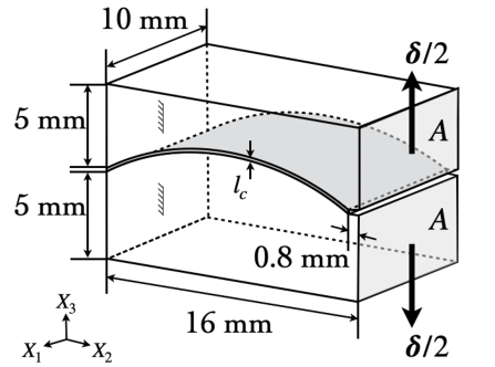
The macroscale material properties are characterized by Young’s modulus ${}^{0}E=210\times 10^{3}\text{ MPa}$, shear modulus ${}^{0}\mu=72\times 10^{3}\text{ MPa}$, bulk modulus ${}^{0}\kappa=167\times 10^{3}\text{ MPa}$, and Poisson’s ratio ${}^{0}\nu=0.29$. The macroscale mesh consists of 3,210 nodes, 14,609 linear tetrahedral finite elements, 320 cohesive elements, and 8,860 Degrees of Freedom (DOFs). This configuration is determined through the mesh refinement study using FM with a varying number of cohesive elements (i.e., from 192 to 572).

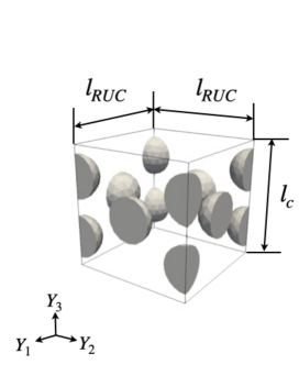
In the next step, we attach 320 RUCs to the material points on the adhesive surface, with each RUC paired with a corresponding cohesive element. For the RUCs, we adopt the material properties of the surrogate model detailed in [52, 40], which consists of stiff nylon particles [43] embedded in a polyurethane structural adhesive [16] as shown in Fig. 5. Each RUC measures $100\times 100\times 100\,\mu\text{m}^{3}$, and includes 4 particles with a diameter of 18.2 $\mu$m resulting in a particle volume fraction of $c_{p}=10.10\,\%$. Particle packing is arranged to maintain axial symmetry about the $Y_{3}$ axis in this verification example. The thickness of the adhesive layer is denoted as $l_{c}=100\,\mu\text{m}$. The size of each RUC, $l_{RUC}=100\;\mu$m, is determined through independent numerical simulations as in [52]. The macroscopic loading rate is restricted to $\|\llbracket{}^{0}\dot{\vec{u}}\,\rrbracket/l_{c}\|\leq 1.0\,\text{s}^{-1}$ due to the relatively low rate sensitivity of the adhesive materials. The material properties of the split damage model (see Lee et al. [40]) are given in Table 1. We note that damage propagation does not occur within the stiff nylon particles.

Table 1: Material properties of the particles and matrix. $Y_{in}$ is the initial damage threshold, $p_{1}$ and $p_{2}$ are damage parameters, and $\mu^{*}$ denotes the damage viscosity.

	$E$ [MPa]	$\mu^{*}$ [MPa]	$\kappa$ [MPa]	$\nu$ [-]	$Y_{in}$ [MPa]	$p_{1}$ [-]	$p_{2}$ [-]	$\mu^{*}$ [s-1]
Particle	$2.40\times 10^{3}$	$8.96\times 10^{2}$	$2.50\times 10^{3}$	0.34	-	-	-	-
Matrix	$8.00\times 10^{2}$	$2.99\times 10^{2}$	$8.33\times 10^{2}$	0.34	0.15	8.0	2.5	100.0

The RUC is discretized with 4,004 nodes, 23,344 finite elements, and 11,586 DOFs with an average mesh size of $3.5\,\mu\text{m}$. This configuration is obtained from a mesh convergence study solving Eq. (5), using uniaxial tensile and pure shear loading conditions for FM. The average mesh size is progressively adjusted to $3.5$, $2.8$, and $1.9$ $\mu$m, demonstrating solution convergence. We further conduct tensile loading using FM to determine the optimal size of each microscale server $\mathcal{S}_{i}$ (not presented for brevity). This strong scaling study shows near-ideal speedup with 4 cores. Thus, we allocate 4 cores to each $\mathcal{S}_{i}$. In general, multiscale_net allows for non-uniform recourse allocation. However, in this work, we assign the same number of cores to each server as both FM and TM are locally parallelized.

Leveraging the chosen mesh size and resource allocation, we assign the maximum jump displacement to be $\lambda=0.1\times l_{c}$ (see Eq. (21)) as the traction-separation relation predicts complete material failure at 10% elongation [52]. We discretize this jump into $N_{s}=100$ segments and generate $N_{t}\in[100,\,1000]$ training samples for each segment. Also, we exploit the geometric symmetry of the RUC by substituting $\phi_{i}=\frac{\pi}{4}H^{i}_{1}$ in Eq. (22) to assess the density of $\mathcal{DB}$ (see Section 3). In the computational environment, we employ job arrays utilizing a total of 272 cores to build $\mathcal{DB}$ in parallel.

Figure 6: Classification error for nonlinear classifiers trained on data with varying model tolerances of $\gamma=10\%$, 15%, and 20%.

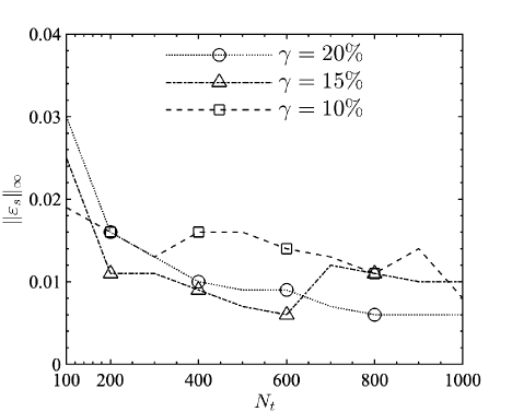
To address the impact of $N_{t}$ in Eq. (16) for each segment, $s$, on the accuracy of the SVM classifier, we define the segment classification error

$$\varepsilon_{s}=\frac{N^{i}}{N_{\text{C}}},$$ (31)

where $N^{i}$ denotes the number of incorrect classifications and $N_{C}(\phi,\theta)$ represents the number of classifications (i.e., testing samples), which remains constant for each segment. For this error analysis, we generated $N_{C}=1000$ quasi-random testing samples, $(\phi,\theta)$, that are independent of the training samples, $N_{t}$.

Fig. 6 demonstrates the maximum classification error for all segments $s$ during the loading history up to the maximum displacement jump of $\lambda=0.1\times l_{c}$. We can see that error drops quickly and remains relatively constant for a database with $N_{t}\geq 500$ for the nonlinear SVM classifier with modeling error tolerance $\gamma=10\%,\,15\%,\,\text{and }20\%$. For all cases, we misclassified less than 1.8% of tests. Based on these observations, we set $N_{t}=500$ for the adaptive multiscale simulations to follow. Consequently, we obtain a database $\mathcal{DB}=\left\{f_{1},f_{2},\cdots,f_{N_{s}}\right\}$ by assessing $N_{s}=100$ radial distances, $r$, based on Eq. (21).

Figure 7: An offline database trained on $N_{t}=500$ samples and $r=30$% elongation with $\gamma=15$% model tolerance. (a) 3D jump displacement space and (b) 2D spherical coordinate system.

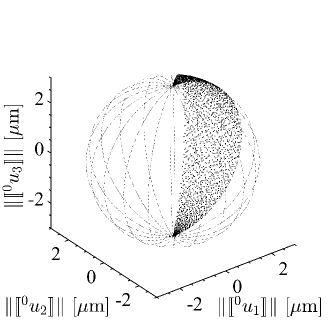
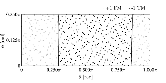
Fig. 7 illustrates an offline database trained on $N_{t}=500$ samples and $r=30$% elongation (i.e., $r=0.3\lambda$) with $\gamma=15$% model tolerance. Fig. 7 shows the decision boundary created by SVR in a 2D spherical coordinate system, with dense clusters removed to ensure even sampling. Moreover, we note that the less expensive TM covers a large range of loading conditions. This illustrates the possible modeling acceleration by adaptively selecting TM over FM with a user prescribed tolerance $\gamma$.

As an initial condition, adaptive multiscale simulation starts always using TM, adaptively changing to FM based on $\mathcal{DB}$. The remaining figures present DCB results from adaptive multiscale simulations using a total of 272 cores. We establish 64 microscale servers $\mathcal{S}_{i}$, each with 4 cores per server, based on the strong scaling study, with a total of 256 cores. This enables multiscale_net to balance the work of the adaptive simulations as shown in Fig. 4. The remaining 16 cores were allocated to the macroscale domain $\mathcal{D}_{0}$.

Figure 8: Adaptive multiscale results for the DCB test. (a) The $F$–$\delta$ response, and (b) the ratio of TM versus FM cohesive elements during the simulation.

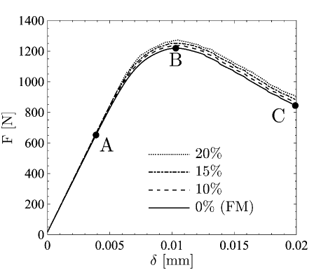
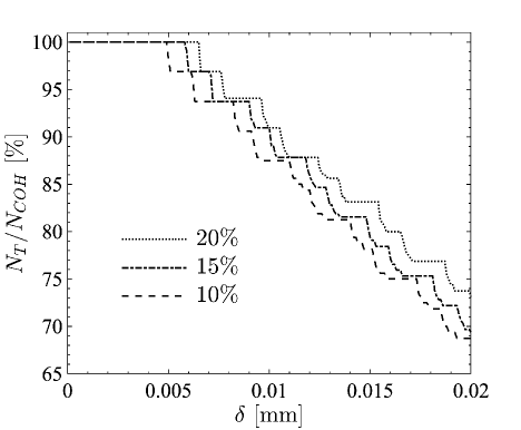
Fig. 8 shows the $F-\delta$ response for different $\gamma$ values. The difference in the peak load between FM and each adaptive simulation is 1.40% for $\gamma=10\%$, 2.65% for $\gamma=15\%$, and 4.38% for $\gamma=20\%$, respectively. We note that $\gamma=0\%$ represents the FM simulation. Over the loading history, the adaptive strategy progressively adds more FM cells to improve accuracy in the adhesive layer as damage in the RUCs evolves. Fig. 8 displays the percent ratio of TM versus FM cohesive elements (i.e., RUCs) with different $\gamma$ values. For the initial loading history, $\delta\lesssim 0.005$ mm, the cell response is hyper-elastic and the algorithm does not adapt from TM. The adaptive simulation with the tighter $\gamma$ tolerance adapts earlier and progressively switches from TM to FM as damage propagates in the adhesive layer. The stepwise nature of the adaption is due to the front propagating over cohesive elements at the interface (see Fig. 9).

Figure 9: The magnitude of the cohesive traction vector for $\gamma=0\%$ (FM) at the points marked in Fig. 8.

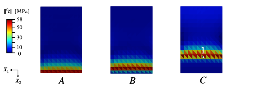
Fig. 9 presents the magnitude of the traction vectors, computed using Eq. (8), at specific points along the loading history identified in Fig. 8. These points correspond to the proportional limit (A), the peak load (B), and the progressive damage state at the end of the simulation (C). To assess the impact of modeling tolerance $\gamma$ on the adhesive response, we analyze the macroscopic traction vector error

$$\varepsilon_{\vec{t}} =\frac{\|{}^{0}\vec{t}_{FM}-{}^{0}\vec{t}\|}{\|{}^{0}\vec{t}_{FM}\|_{\infty}}\times 100\%.$$ (32)

Fig. 10 shows the traction vector error for $\gamma=15\%$ and $\gamma=10\%$ values. The error drops precipitously as the modeling tolerance approaches FM (i.e., full PDE solution).

Figure 10: The traction vector error at the end of the loading history for (a) $\gamma=15$% and (b) $\gamma=10$%.

Table 2: The speedup of adaptive multiscale simulations.

$\gamma$ [%]	$N_{T}/N_{COH}$	$T_{FM}/T_{AM}$
20	0.731	1.55
15	0.694	1.42
10	0.488	1.33

To assess the savings in simulation time, we compute the speedup ratio $T_{FM}/T_{AM}$, where $T_{FM}$ represents the runtime of the FM simulation, and $T_{AM}$ denotes the runtime of the adaptive multiscale simulations, respectively. As expected, the large error tolerance leads to large time savings, as depicted in Table 2.

Figure 11: The DCB macroscale and microscale results at point C in Fig. 8. (a) The stress component $\sigma_{33}$ in the deformed configuration (deformations magnified 50$\times$) and (b) damage pattern in the RUC. The cell location is depicted in Fig. 9.

Figure 12: Strong scaling of the multiscale simulations.

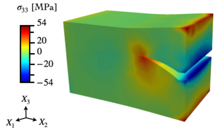
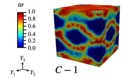
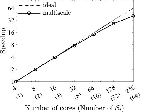
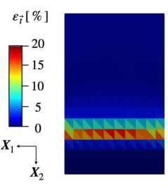
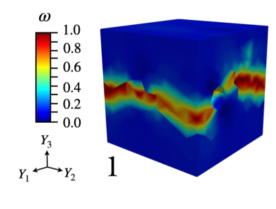
Fig. 11 shows the 33 Cauchy stress tensor component in the deformed configuration. There is a large stress concentration at the crack tip. We note that stress concentrations on the face $A$ of the beam are the result of the prescribed boundary conditions. The face $A$ is not allowed to rotate during the beam loading. Fig. 11 displays the damage pattern in the microstructure at the end of the loading history for the cell behind the crack front (see white marker $3$ in Fig. 9). The cell failed progressively around the particles and close to the top and bottom adherends.

Fig. 12 shows the strong scaling achieved by the multiscale_net library for the multiscale simulations with $\gamma=0$%. The computational speedup is defined as $\nicefrac{{t_{n}}}{{t_{N}}}$, where $t_{N}$ is the time to compute the simulation using $N$ resources (e.g., microscale servers, $\mathcal{S}_{i}$) and $t_{n}$ is the time to compute the same simulation with more resources, $n$. In our case, we start with one micro-server $\mathcal{S}_{1}$ consisting of 4 cores and increase the computational resources to 64 micro-servers with 256 cores in total. The multiscale_net retains a near ideal $64\times$ speedup for the full computational allocation.

6.2 Ultimate static test of National Rotor Testbed

In the second example, we model the geometry of a 13-meter NRT blade that was tested by NREL [25, 54, 34]. In particular, we aim to predict the ultimate bending moment that was experimentally measured as 228.7 kN$\cdot$m. In this work, we assume that ultimate failure starts at the adhesive layer. Thus, we associate ultimate failure with fully failed RUCs, which indicates crack propagation. Therefore, we compute the ultimate moment, $M^{h}$, as a moment where the jump opening displacement $\|\llbracket{}^{0}\vec{u}\,\rrbracket\|$ starts rapidly growing (i.e., the adhesive layer starts opening and the crack starts propagating).

Figure 13: NRT wind turbine blade. (a) Geometry and boundary conditions. (b) RUC of the adhesive layer with manufacturing defects (i.e., voids)

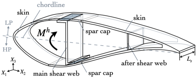
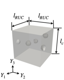
Fig. 13 depicts the blade geometry, replicating the S814 airfoil section with a chordline width of 1.450 m and a span-wise length of $L_{s}=0.20$ m. We focus on the spanwise section from 2.7 to 2.9 meters, because the blade failed near the 2.9 m station as reported in [25]. The span-wise length of $L_{s}=0.2$ m was selected based on the blade uniformity. Moreover, we have performed independent numerical simulations to confirm that this span-wise length does not influence the multiscale simulation results (i.e., $L_{s}$ of 0.25 m and 0.20 m yield identical results). The low-pressure side is denoted as LP and the high-pressure side as HP.

The root of the blade (i.e., $X_{1}=0$) is clamped to simulate fixed boundary conditions. We impose a bending moment $M^{h}$ about $X_{2}$ to introduce a constant bending stress and replicate the loading conditions introduced in the NREL report [25]. Specifically, we compute the neutral axis of the cross-section and its principal axes. Next, we apply the bending moment as a traction vector, $\hat{\vec{t}}=(\hat{t}_{X_{1}},0,0)^{\top}$, in the $X_{1}$ direction computed from the standard flexure formula for unsymmetric bending. The $X_{1}$ component of the traction vector reads

$$\hat{t}_{X_{1}}=\frac{M_{X_{2}}^{{}^{\prime}}X_{3}^{{}^{\prime}}}{I_{X_{2}}^{{}^{\prime}}}-\frac{M_{X_{3}}^{{}^{\prime}}X_{2}^{{}^{\prime}}}{I_{X_{3}}^{{}^{\prime}}},$$ (33)

where $X_{2}^{{}^{\prime}}$ and $X_{3}^{{}^{\prime}}$ are the principal axes of the cross-section, $I_{X_{2}}^{{}^{\prime}}$ and $I_{X_{3}}^{{}^{\prime}}$ represent the principle moments of area, and $M^{h}=\sqrt{(M_{X_{2}}^{{}^{\prime}})^{2}+(M_{X_{3}}^{{}^{\prime}})^{2}}$. The applied moment, $M^{h}$, increases linearly from 0.0 to 250.0 kN$\cdot$m over a span of of 60 seconds to ensure the quasi-static loading condition. In our simulations, we prevent warping (i.e., deplanation) of the cross-section at $X_{1}=0.2$ m (i.e., the cross-section remains planar). Moreover, we ignore the torque moment on the blade as it is small, and allow the cross-section at $X_{1}=0.2$ m to rotate freely around any axis.

Table 3: Material properties of the NRT wind turbine blade.

	${}^{0}E$ [MPa]	${}^{0}\mu^{*}$ [MPa]	${}^{0}\kappa$ [MPa]	${}^{0}\nu$ [-]
Spar cap	$12.0\times 10^{3}$	$3.70\times 10^{3}$	$8.70\times 10^{3}$	0.27
Shear web	$5.43\times 10^{3}$	$1.97\times 10^{2}$	$3.77\times 10^{3}$	0.26
Skin	$4.91\times 10^{3}$	$1.82\times 10^{2}$	$3.41\times 10^{3}$	0.26

In our constitutive model, we selected [+45/-45] layups of E-glass fiber-reinforced composite materials. The spar caps are designed with a thickness of 11 mm, and the shear webs are set at a thickness of 16.7 mm. The thickness of the skin is established at 15.1 mm. These dimensions are approximated from the actual NRT data. For the shear webs, we utilize volume-averaged effective properties derived from a sandwich structure core of end-grain balsa wood as detailed in [55]. The macroscale material properties of the E-glass fiber-reinforced composites and sandwich structures used in our simulations are summarized in Table 3.

Figure 14: A section of the mesh highlighting the main shear web. Point $A$ marks the center of the spar cap.

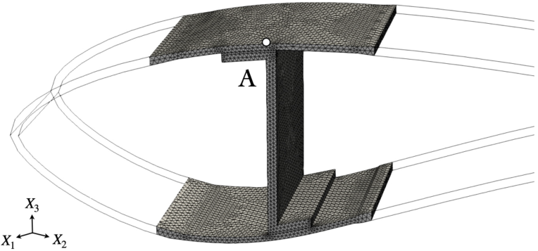
The macroscale mesh of the NRT blade section consists of 37,667 nodes, 156,600 linear tetrahedral finite elements, 954 cohesive elements, and 109,251 DOFs. This mesh configuration is chosen based on the mesh refinement study. We select the macroscopic mesh density so as to capture the main deformation modes. For illustration, Fig. 14 depicts the finite element mesh assigned to the spar caps and the main shear web of the blade section. The center of the spar cap is indicated by a white point labeled $A$.

Figure 15: Calibration of the constitutive model with experimental data for three loading rates.

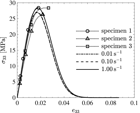
The top and bottom adhesive layers between the spar caps and the main shear web are manufactured from a structural adhesive. The shear web at the trailing edge is assumed to be perfectly bonded to the rest of the blade. Fig. 13 shows an example RUC with dimension of $100\times 100\times 100\,\mu\text{m}^{3}$ which consists of a structural epoxy adhesive containing 4 voids with a diameter of 19.3 $\mu\text{m}$. Volume fraction of the voids is $c_{p}=1.51\%$ and the voids are randomly distributed within each RUC using the packing code $Rocpack$ [66]. The diameters and volume fraction of voids correspond to values of typical manufacturing defects reported in the literature [63]. The material properties are calibrated from experimental data for a structural adhesive epoxy under tensile loading conditions [50]. Fig. 15 shows the normal stress-strain behavior (i.e., $\sigma_{33}$–$e_{33}$) of the epoxy under uniaxial tension at different strain rates. The damage parameters are chosen to ensure that the peak and failure stress fall within the ranges reported in the literature [50, 10]. Table 4 displays material properties calibrated from experimental data.

Table 4: Material properties of the epoxy structural adhesive.

$E$ [MPa]	$\mu^{*}$ [MPa]	$\kappa$ [MPa]	$\nu$ [MPa]	$Y_{in}$ [MPa]	$p_{1}$ [-]	$p_{2}$ [-]	$\mu$ [$\text{s}^{-1}$]
$3.0\times 10^{3}$	$1.1\times 10^{3}$	$3.3\times 10^{3}$	0.35	0.10	10.0	1.1	100.0

Moving forward, a total of 954 RUCs, each linked to a corresponding cohesive element, are allocated to material points on the adhesives. Of these, 520 RUCs are assigned to the upper adhesive near the LP skin, and 434 RUCs to the lower adhesive adjacent to the HP skin. Each RUC includes 1,619 nodes, 9,016 finite elements, and 4,416 DOFs with average element size of $4.8\,\mu\text{m}$. The mesh density is determined by refinement study employing average element sizes from $5.0$ to $4.0\,\mu\text{m}$ under different loading rates of $\|\llbracket{}^{0}{\dot{\vec{u}}}\,\rrbracket/l_{c}\|=1.00,\,0.10,\,\text{and}\,0.01\,\text{s}^{-1}$. Additionally, we allocate 4 computing cores to an RUC based on a strong scaling study. We note that if performed as a single-scale FEM simulation, such a simulation would contain a total of 8,757,864 elements. This would be a large simulation with complicated contiguous meshing between two scales. Such simulations are inherently difficult, especially for highly nonlinear material behavior (e.g., damage).

Figure 16: The classification error for nonlinear classifiers trained on epoxy RUC data with varying model tolerances of $\gamma=3\%$ and 5%.

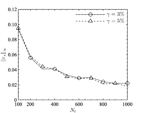
Next, we generate training samples for structural epoxy (i.e., $N_{t}\in[100,\,1000]$) for each segment, along with $N_{c}=1000$ quasi-random testing samples (i.e., classification samples) for each segment. This training sequence is designed to assess the density of the database. Loading is assigned with a maximum elongation of $\lambda=0.05\times l_{c}$ in Eq. (21), based on the observation that the complete failure of the adhesive occurs near the 5% elongation (see Fig. 15). The database, $\mathcal{DB}$, is trained on 1,040 cores. We evaluate the classification error, Eq. (24), of $\mathcal{DB}$ for model tolerances $\gamma=3\%$ and $5\%$, to verify that the density of training samples $N_{t}$ is sufficient. The tighter modeling tolerance $\gamma$ is important in this example, because the response of the RUCs is shear-dominated.

Figure 17: An offline database with $r=30$% elongation for epoxy RUC with $\gamma=5$% model tolerance. (a) 3D jump displacement space. (b) 2D spherical coordinate system.

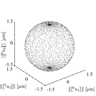
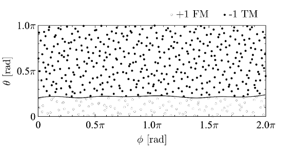
Fig. 16 shows the classification error for both $\gamma$ values and we select $N_{t}=500$ for further adaptive multiscale simulations. In this case we misclassified less than 3.8% of samples. Fig. 17 shows the database for $r=30$% elongation with $\gamma=5$% modeling tolerance. As can be seen, a large portion of the $(\phi,\theta)$ space can be modeled using TM.

Figure 18: Validation of the adaptive multiscale simulations. (a) Bending moment versus the micro-strain. (b) Ultimate bending moment. Note that the micro-strain is computed as $\varepsilon_{\mu}=\varepsilon_{b}\times 10^{6}$.

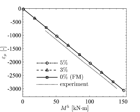
The multiscale simulations are executed on 1,040 cores, with 1,024 cores dedicated to microscale servers and 16 cores allocated to the macroscale domain. The simulations are validated against the experimental measurements of micro-strain and the ultimate bending moment. The micro-strain $\varepsilon_{\mu}$ is measured by a strain gauge mounted on the spar cap at the 2.9 m station. In our simulations, we compute the bending strain using curvature

$$\varepsilon_{b}=-\frac{l_{X_{3}}}{\rho_{b}},$$ (34)

where $l_{X_{3}}$ is the distance from the neutral axis and $\rho_{b}$ is the local radius of curvature. Taking the bending profile to be the arc of a circle, we compute the radius of curvature as $\rho_{b}=\nicefrac{{L_{s}}}{{\zeta}}$, where $\zeta$ is the central angle. The central angle is estimated in the $X_{1}-X_{3}$ plane from the displacement data around the neutral axis using a small angle approximation. We use 19 points and compute the central angle as $\zeta\approx\nicefrac{{\sqrt{{}^{0}u_{1}^{2}+{}^{0}u_{3}^{2}}}}{{L_{s}}}$. The maximum value does not exceed $\rho_{b}(\max)=$ 0.0038 radians. The micro-strain is computed at the marked point $A$ in Fig. 14 and compared with the experimental data in Fig. 18. We note the excellent agreement between the simulations and experiments with micro-strain error in $\varepsilon_{\mu}$ of $\approx 150$. The micro-strain measurement was reported up to the applied moment $M^{h}=$ 140 kN$\cdot$m, which is within the hyper-elastic response of the blade. Thus, the $\gamma$ tolerance does not the impact the results.

Figure 19: Low-pressure side adhesive layer. (a) Magnitude of the traction vector at point A in Fig. 18. (b) Localized microscale damage pattern at the marked material point 1 in Fig. 19.

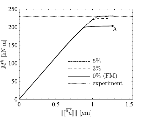
Next, we validate the multiscale simulations against the ultimate moment. Fig. 18 shows the applied moment as a function of the jump displacement. We compute the jump displacement as an average over the cohesive elements in the first row of the adhesive layer at the low-pressure interface (see Fig. 19 for discretization of the interface). When the blade failed catastrophically at the 2.9 m station, the applied bending moment was 228.7 kN$\cdot$m. Our multiscale simulations with FM predict an ultimate moment of 203 kN$\cdot$m (see Fig. 18). That is only 11.2% error compared to the experimental measurement. Considering the complexity of both the experiment and the multiscale simulations, such a small error is very impressive. Both adaptive multiscale simulations over-predict the FM results but are closer to the experimental measurement.

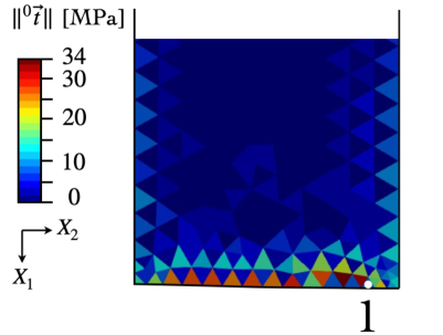
Fig. 19 displays the norm of the traction vector and the damage pattern in the failed RUC. We note that the RUCs fail mostly in shear (see Fig. 19). In our work, the failure of a cohesive element (i.e., RUC) is characterized by the point where the magnitude of the displacement jump satisfies $\|\llbracket{}^{0}\vec{u}\,\rrbracket\|\geq 3\,\mu\text{m}$. This captures nearly the entire material response as shown in Fig. 15 (i.e. $e_{33}\geq$ 0.03 for complete failure). We note that only a small number of cohesive elements fail, but even this small number is enough to initiate rapid opening of the adhesive layer without an increase in bending moment as depicted in Fig. 18. For $\gamma$ = 5%, 3%, and 0% (i.e., FM) models, we have detected 2, 4, and 3 fully failed cohesive elements, respectively.

Figure 20: Average traction-separation response of failed cohesive elements based on the modeling tolerance.

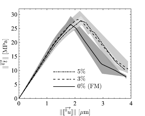
Fig. 20 shows the averaged traction-separation response with the observed spread among elements represented by different shades of gray around the mean. The gray regions are represented by min/max values for the individual $\gamma$ simulations. As expected, the maximum averaged traction vector values are similar to the maximum stress values in Fig. 15.

Table 5: The speedup of adaptive multiscale simulations of NRT blade.

$\gamma$ [%]	$N_{T}/N_{COH}$	$T_{FM}/T_{AM}$
5	0.9937	2.75
3	0.9895	2.45

Next, we present the acceleration data for our adaptive simulations. Table 5 shows speedup and the ratio of TM versus FM. We can see that the speedup is quite large compared to that of the DCB example presented in Section 6.1. We also note that introducing a third model (e.g., a phenomenological cohesive law) would further accelerate the multiscale simulations.

Figure 21: Macroscopic response of the NRT blade. (a) Stress component in the $X_{1}$ direction. (b) Displacement component in the $X_{1}$ direction.

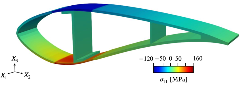
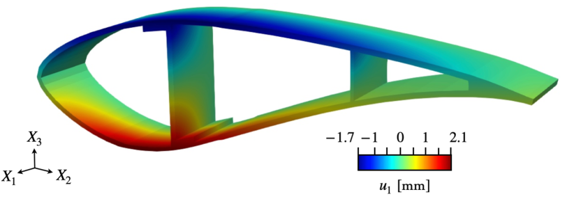
We conclude this example with the macroscopic response of the NRT blade at the end of the loading history (see marked point A in Fig. 18). Fig. 21 displays the $\sigma_{11}$ component of the Cauchy stress tensor and the $u_{1}$ component of the displacement vector, respectively. Tensile stress of $\approx 160$ MPa and compressive stress of $\approx 120$ MPa are observed at the high-pressure and low-pressure sides of the blade. As expected, the most stress is carried by the spar caps above the main shear web. The skin also carries some load, but the trailing edge is mostly stress-free. The blade deformation is quite nonuniform, with the leading and trailing edges deforming slightly as they are both close to the neutral axis. We note again that the shear web at the trailing edge is perfectly bonded to the rest of the structure.

7 Conclusion

We present a new adaptive and parallel multiscale solver for large-scale engineering applications, leveraging support vector regression and a new networking library. This adaptive approach utilizes computational homogenization of interfaces and two microscale models based on an offline database to predict highly nonlinear material behavior across scales, thereby reducing computational time while ensuring high-fidelity results. Our networking library facilitates the dynamic selection of microscale models within a high-performance computing setting, significantly enhancing simulation feasibility. The hierarchically parallel multiscale solver is carefully verified and subsequently validated for a large engineering problem. In particular, we simulate a complex real-world engineering application involving the ultimate failure of a large wind turbine blade. This work represents an advancement in multiscale simulations, offering a comprehensive solution to computational multiscale demands both through model selection and high-performance computing. Finally, we highlight the potential for introducing a whole library of models (i.e., phenomenological, ROM, etc.) that could be considered in future studies to improve computational performance while retaining the predictability of industrially relevant large multiscale simulations.

References

- [1] I. Babuška. Solution of interface problems by homogenization - III. SIAM Journal on Mathematical Analysis, 8(6):923–937, 1977.
- [2] P.L. Bartlett, S. Boucheron, and G. Lugosi. Model selection and error estimation. Machine Learning, 48(1):85–113, 2002.
- [3] P.T. Bauman, J.T. Oden, and S. Prudhomme. Adaptive multiscale modeling of polymeric materials with arlequin coupling and goals algorithms. Computer methods in applied mechanics and engineering, 198(5-8):799–818, 2009.
- [4] A. Beel and J. Fish. Solver-free reduced order homogenization for nonlinear periodic heterogeneous media. Computer Methods in Applied Mechanics and Engineering, 425:116932, 2024.
- [5] A. Benssousan, J.L. Lions, and G. Papanicoulau. Asymptotic Analysis for Periodic Structures. North-Holland, Amsterdam-New York-Oxford, 1978.
- [6] S. Bhattacharjee and K. Matouš. A nonlinear manifold-based reduced order model for multiscale analysis of heterogeneous hyperelastic materials. Journal of Computational Physics, 313:635–653, 2016.
- [7] S. Bhattacharjee and K. Matouš. A nonlinear data-driven reduced order model for computational homogenization with physics/pattern-guided sampling. Computer Methods in Applied Mechanics and Engineering, 359:112657, 2020.
- [8] D. Bishara, Y. Xie, W.K. Liu, and S. Li. A state-of-the-art review on machine learning-based multiscale modeling, simulation, homogenization and design of materials. Archives of Computational Methods in Engineering, 30(1):191–222, 2023.
- [9] P.R. Budarapu, R. Gracie, S.P.A. Bordas, and T. Rabczuk. An adaptive multiscale method for quasi-static crack growth. Computational Mechanics, 53:1129–1148, 2014.
- [10] T. Carlberger, A. Biel, and U. Stigh. Influence of temperature and strain rate on cohesive properties of a structural epoxy adhesive. International Journal of Fracture, 155(2):155–166, 2009.
- [11] P.P. Castañeda. Second-order homogenization estimates for nonlinear composites incorporating field fluctuations: I theory. Journal of the Mechanics and Physics of Solids, 50(4):737–757, 2002.
- [12] S. Chan and A.H. Elsheikh. A machine learning approach for efficient uncertainty quantification using multiscale methods. Journal of Computational Physics, 354:493–511, 2018.
- [13] E. Chung, Y. Efendiev, and T.Y. Hou. Adaptive multiscale model reduction with generalized multiscale finite element methods. Journal of Computational Physics, 320:69–95, 2016.
- [14] C. Cortes and V. Vapnik. Support-vector networks. Machine learning, 20:273–297, 1995.
- [15] P.C. Deka and S.R. Naganna. Support vector machine applications in the field of hydrology: a review. Applied soft computing, 19:372–386, 2014.
- [16] C. Di Fratta, M. Zivaljic, A. Corsaro, D. Hofstetter, M. Schlumpf, B. Bosshard, and F. Choffat. Structural adhesives with customized fast curing. Adhes. Adhes. Sealants., 17:18–23, 2020.
- [17] H. Drucker, C.J. Burges, L. Kaufman, A. Smola, and V. Vapnik. Support vector regression machines. Advances in neural information processing systems, 9, 1996.
- [18] J.D. Eshelby. The determination of the elastic field of an ellipsoidal inclusion. Proceedings of the royal society of London. Series A. Mathematical and physical sciences, 241:376–396, 1957.
- [19] R. Fan, Z. Yuan, and J. Fish. Adaptive two-scale nonlinear homogenization. International Journal for Computational Methods in Engineering Science and Mechanics, 11(1):27–36, 2010.
- [20] R.E. Fan, P.H. Chen, C.J. Lin, and T. Joachims. Working set selection using second order information for training support vector machines. Journal of machine learning research, 6(12), 2005.
- [21] F. Feyel and J.L. Chaboche. Fe2 multiscale approach for modelling the elastoviscoplastic behaviour of long fibre sic/ti composite materials. Computer methods in applied mechanics and engineering, 183(3-4):309–330, 2000.
- [22] J. Fish. Multiscale methods: bridging the scales in science and engineering. Oxford University Press, 2009.
- [23] J. Fish, G.J. Wagner, and S. Keten. Mesoscopic and multiscale modelling in materials. Nature Materials, 20(6):774–786, 2021.
- [24] R. Fletcher. Practical methods of optimization. John Wiley & Sons, 2000.
- [25] B. Gage, R. Beach, and S. Hughes. Laboratory wind turbine blade static testing of the sandia national rotor testbed 13-meter wind turbine blade. Technical report, National Renewable Energy Lab.(NREL), Golden, CO (United States), 2021.
- [26] M.G.D. Geers, V.G. Kouznetsova, and W.A.M. Brekelmans. Multi-scale computational homogenization: Trends and challenges. Journal of computational and applied mathematics, 234(7):2175–2182, 2010.
- [27] M.G.D. Geers, V.G. Kouznetsova, K. Matouš, and J. Yvonnet. Homogenization methods and multiscale modeling: non-linear problems. In E. Stein, R. de Borst, and T.J.R. Hughes, editors, Encyclopedia of Computational Mechanics, chapter in press. John Wiley and Sons, NY, 2004.
- [28] S. Ghosh, K. Lee, and S. Moorthy. Two scale analysis of heterogeneous elastic-plastic materials with asymptotic homogenization and Voronoi cell finite element model. Computer Methods in Applied Mechanics and Engineering, 132:63–116, 1996.
- [29] S. Ghosh, K. Lee, and P. Raghavan. A multi-level computational model for multi-scale damage analysis in composite and porous materials. International Journal of Solids and Structures, 38(14):2335–2385, 2001.
- [30] J.H. Halton. On the efficiency of certain quasi-random sequences of points in evaluating multi-dimensional integrals. Numerische Mathematik, 2:84–90, 1960.
- [31] M.A. Hearst, S.T. Dumais, E. Osuna, J. Platt, and B. Scholkopf. Support vector machines. IEEE Intelligent Systems and their applications, 13(4):18–28, 1998.
- [32] R. Hill. On constitutive macro-variables for heterogeneous solids at finite strain. Proceedings of the Royal Society of London. A. Mathematical and Physical Sciences, 326(1565):131–147, 1972.
- [33] C.B. Hirschberger, S. Ricker, P. Steinmann, and N. Sukumar. Computational multiscale modelling of heterogeneous material layers. Engineering Fracture Mechanics, 76(6):793–812, 2009.
- [34] C.L. Kelley. Aerodynamic design of the national rotor testbed. Technical report, Sandia National Lab.(SNL-NM), Albuquerque, NM (United States), 2015.
- [35] Z.F. Khisaeva and M. Ostoja-Starzewski. On the size of RVE in finite elasticity of random composites. Journal of Elasticity, 85(2):153–173, 2006.
- [36] L. Kocis and W.J. Whiten. Computational investigations of low-discrepancy sequences. ACM Transactions on Mathematical Software (TOMS), 23(2):266–294, 1997.
- [37] M.G. Kulkarni, P.H. Geubelle, and K. Matouš. Multi-scale modeling of heterogeneous adhesives: Effect of particle decohesion. Mechanics of Materials, 41(5):573–583, 2009.
- [38] M.G. Kulkarni, K. Matouš, and P.H. Geubelle. Coupled multi-scale cohesive modeling of failure in heterogeneous adhesives. International Journal for Numerical Methods in Engineering, 84(8):916–946, 2010.
- [39] B.A. Le, J. Yvonnet, and Q.C. He. Computational homogenization of nonlinear elastic materials using neural networks. International Journal for Numerical Methods in Engineering, 104(12):1061–1084, 2015. nme.4953.
- [40] S. Lee, K. Ramos, and K. Matouš. Numerical study of damage in particulate composites during high-strain rate loading using novel damage model. Mechanics of Materials, 160:103944, 2021.
- [41] F.T. Leighton. A graph coloring algorithm for large scheduling problems. Journal of research of the national bureau of standards, 84(6):489–506, 1979.
- [42] H.J. Logarzo, G. Capuano, and J.J. Rimoli. Smart constitutive laws: Inelastic homogenization through machine learning. Computer Methods in Applied Mechanics and Engineering, 373:113482, 2021.
- [43] C.B.B. Luna, E.A.S. Filho, D.D. Siqueira, E.M. Araújo, E.P. Nascimento, and T.J.A. de Mélo. Influence of small amounts of abs and abs-ma on pa6 properties: Evaluation of torque rheometry, mechanical, thermomechanical, thermal, morphological, and water absorption kinetics characteristics. Materials, 15(7):2502, 2022.
- [44] S. Makridakis, E. Spiliotis, and V. Assimakopoulos. Statistical and machine learning forecasting methods: Concerns and ways forward. PloS one, 13(3):e0194889, 2018.
- [45] K. Matouš, M.G.D. Geers, V.G. Kouznetsova, and A. Gillman. A review of predictive nonlinear theories for multiscale modeling of heterogeneous materials. Journal of Computational Physics, 330:192–220, 2017.
- [46] K. Matouš, M.G. Kulkarni, and P.H. Geubelle. Multiscale cohesive failure modeling of heterogeneous adhesives. Journal of the Mechanics and Physics of Solids, 56(4):1511–1533, 2008.
- [47] J.C. Michel, H. Moulinec, and P. Suquet. Effective properties of composite materials with periodic microstructure: a computational approach. Computer methods in applied mechanics and engineering, 172(1):109–143, 1999.
- [48] J.C. Michel and P. Suquet. Nonuniform transformation field analysis. Int. J. Sol. Struct., 40(25):6937–6955, 2003.
- [49] C. Miehe, J. Schröder, and J. Schotte. Computational homogenization analysis in finite plasticity simulation of texture development in polycrystalline materials. Computer methods in applied mechanics and engineering, 171(3-4):387–418, 1999.
- [50] J.P.R. Monteiro, R.D.S.G. Campilho, E.A.S. Marques, and L.F.M. Da Silva. Experimental estimation of the mechanical and fracture properties of a new epoxy adhesive. Applied Adhesion Science, 3(1):1–17, 2015.
- [51] M. Mosby and K. Matouš. Hierarchically parallel coupled finite strain multiscale solver for modeling heterogeneous layers. International Journal for Numerical Methods in Engineering, 102(3-4):748–765, 2015.
- [52] M. Mosby and K. Matouš. On mechanics and material length scales of failure in heterogeneous interfaces using a finite strain high performance solver. Modelling and Simulation in Materials Science and Engineering, 23(8):085014, 2015.
- [53] M. Mosby and K. Matouš. Computational homogenization at extreme scales. Extreme Mechanics Letters, 6:68–74, 2016.
- [54] R.E. Murray, J. Roadman, and R. Beach. Fusion joining of thermoplastic composite wind turbine blades: Lap-shear bond characterization. Renewable Energy, 140:501–512, 2019.
- [55] A.N. Norris. A differential scheme for the effective moduli of composites. Mechanics of materials, 4(1):1–16, 1985.
- [56] J.T. Oden and K.S. Vemaganti. Estimation of local modeling error and goal-oriented adaptive modeling of heterogeneous materials: I. error estimates and adaptive algorithms. Journal of Computational Physics, 164(1):22–47, 2000.
- [57] J.T. Oden and T.I. Zohdi. Analysis and adaptive modeling of highly heterogeneous elastic structures. Computer Methods in Applied Mechanics and Engineering, 148(3):367 – 391, 1997.
- [58] C. Oskay and J. Fish. Eigendeformation-based reduced order homogenization for failure analysis of heterogeneous materials. Computer Methods in Applied Mechanics and Engineering, 196(7):1216–1243, 2007.
- [59] G.C.Y. Peng, M. Alber, A.B. Tepole, W.R. Cannon, S. De, S. Dura-Bernal, K. Garikipati, G. Karniadakis, W.W. Lytton, P. Perdikaris, L. Petzoldj, and E. Kuhl. Multiscale modeling meets machine learning: What can we learn? Archives of Computational Methods in Engineering, pages 1–21, 2020.
- [60] D. Rypl. Sequential and parallel generation of unstructured 3D meshes. Czech Technical University, Prague., 1998.
- [61] D. Rypl and Z. Bittnar. Hybrid method for generation of quadrilateral meshes. Engineering Mechanics, 9(1/2):49–64, 2002.
- [62] G. Sachs. Zur ableitung einer fliessbedingung. Z. Ver, Dtsch. Ing., 72:734–736, 1928.
- [63] A. Sánchez Cebrián, F. Klunker, and M. Zogg. Modeling of void formation during the curing process of paste adhesives. Journal of Adhesion Science and Technology, 28(7):731–747, 2014.
- [64] E. Sanchez-Palencia. Non-homogeneous media and vibration theory. In Lecture Notes in Physics, volume 127. Springer-Verlag, 1980.
- [65] T. Schlick, S. Portillo-Ledesma, M. Blaszczyk, L. Dalessandro, S. Ghosh, K. Hackl, C. Harnish, S. Kotha, D. Livescu, A. Masud, K. Matouš, A. Moyeda, C. Oskay, and J. Fish. A multiscale vision-illustrative applications from biology to engineering. International Journal for Multiscale Computational Engineering, 19(2):39–73, 2021.
- [66] D.S. Stafford and T.L. Jackson. Using level sets for creating virtual random packs of non-spherical convex shapes. Journal of computational Physics, 229(9):3295–3315, 2010.
- [67] I. Steinwart and A. Christmann. Support vector machines. Springer Science & Business Media, 2008.
- [68] W. Subber, A. Salvadori, S. Lee, and K. Matouš. Uncertainty quantification of the reverse Taylor impact test and localized asynchronous space-time algorithm. AIP Conference Proceedings, 1979(1):140005, 07 2018.
- [69] G.I. Taylor. Plastic strain in metals. J. Inst. Metals, 62:307–324, 1938.
- [70] I. Temizer and T.I. Zohdi. A numerical method for homogenization in non-linear elasticity. Computational Mechanics, 40:281–298, 2007.
- [71] K. Terada, M. Hori, T. Kyoya, and N. Kikuchi. Simulation of the multi-scale convergence in computational homogenization approaches. International Journal of Solids and Structures, 37(16):2285–2311, 2000.
- [72] R.A. van Tuijl, C. Harnish, K. Matouš, J.J.C. Remmers, and M.G.D. Geers. Wavelet based reduced order models for microstructural analyses. Computational Mechanics, 63(3):535–554, 2019.
- [73] K.S. Vemaganti and J.T. Oden. Estimation of local modeling error and goal-oriented adaptive modeling of heterogeneous materials: Part ii: a computational environment for adaptive modeling of heterogeneous elastic solids. Computer Methods in Applied Mechanics and Engineering, 190(46-47):6089–6124, 2001.
- [74] K. Wang and W.C. Sun. A multiscale multi-permeability poroplasticity model linked by recursive homogenizations and deep learning. Computer Methods in Applied Mechanics and Engineering, 334:337–380, 2018.
- [75] X. Wang and F.J. Hickernell. Randomized halton sequences. Mathematical and Computer Modelling, 32(7-8):887–899, 2000.
- [76] J.R. Willis. Bounds on self-consistent estimates for the overall properties of anisotropic composites. Journal of the Mechanics and Physics of Solids, 25:185–202, 1977.
- [77] J. Yvonnet and Q.C. He. The reduced model multiscale method for the non-linear homogenization of hyperelastic media at finite strains. Journal of Computational Physics, 223:341–368, 2007.