Kermut: Composite kernel regression for protein variant effects
Abstract
Reliable prediction of protein variant effects is crucial for both protein optimization and for advancing biological understanding. For practical use in protein engineering, it is important that we can also provide reliable uncertainty estimates for our predictions, and while prediction accuracy has seen much progress in recent years, uncertainty metrics are rarely reported. We here provide a Gaussian process regression model, Kermut, with a novel composite kernel for modelling mutation similarity, which obtains state-of-the-art performance for protein variant effect prediction while also offering estimates of uncertainty through its posterior. An analysis of the quality of the uncertainty estimates demonstrates that our model provides meaningful levels of overall calibration, but that instance-specific uncertainty calibration remains more challenging. We hope that this will encourage future work in this promising direction.
1 Introduction
Accurately predicting protein variant effects is crucial for both advancing biological understanding and for engineering and optimizing proteins towards specific traits. Recently, much progress has been made in the field as a result of advances in machine learning-driven modeling [1, 2, 3], data availability [4], and relevant benchmarks [5, 6].
While prediction accuracy has received considerable attention, the ability to quantify the uncertainties of predictions has been less intensely explored. This is of immediate practical consequence. One of the main purposes of protein variant effect prediction is as an aide for protein engineering and design, to propose promising candidates for subsequent experimental characterization. For this purpose, it is essential that we can quantify, on an instance-to-instance basis, how trustworthy our predictions are. Specifically, in a Bayesian optimization setting, most choices of acquisition function actively rely on predicted uncertainties to guide the optimization, where well-calibrated uncertainties have been show to correlate with optimization performance [7].
Our goal with this paper is to start a discussion on the quality of the estimated uncertainties of protein property predictions. Gaussian Process (GP) regression is a standard choice for uncertainty quantification due to the closed form expression for the posterior. We therefore first ask the question whether state-of-the-art performance can be obtained within the GP framework. We propose a composite kernel that comfortably achieves this goal, and subsequently investigate the quality of the uncertainty estimates from such a model. Our results show that while standard approaches like reliability diagrams give the impression of good levels of calibration, the quantification of per-instance uncertainties is more challenging. We make our model available as a baseline and encourage the community to place greater emphasis on uncertainty quantification in this important domain. Our contributions can be summarized as follow:
-
•
We introduce Kermut, a Gaussian process with a novel composite kernel for modelling mutation similarity, leveraging signals from pretrained sequence and structure models;
-
•
We evaluate this model on the comprehensive ProteinGym substitution benchmark and show that it is able to reach state-of-the-art performance in protein variant effect prediction, outperforming recently proposed deep learning methods in this domain;
-
•
We provide a thorough calibration analysis and show that Kermut provides well-calibrated uncertainties in most cases;
-
•
We demonstrate that our model can be trained and evaluated orders of magnitude faster and with better out-of-the-box calibration than competing methods.
2 Related work
2.1 Protein property prediction
Predicting protein function and properties using machine-learning based approaches continues to be an innovative and important area of research.
Recently, unsupervised approaches have gained significant momentum where models trained in a self-supervised fashion have shown impressive results for zero-shot estimates of protein fitness and variant effects, where the effect of introducing mutations to a reference protein are gauged [3, 8, 9, 10].
Supervised learning remains a crucial method of utilizing experimental data to predict protein fitness. This is particularly valuable when the trait of interest correlates poorly with the evolutionary signals that unsupervised models capture during training or if multiple traits are considered. Supervised protein fitness prediction using machine learning has been explored in detail in [11], where a comprehensive overview can be found. A major change since then is the use of transfer learning via embeddings extracted from self-supervised models, such as protein language models like ESM-2 [12] and ProtTrans [13]. In [14], the authors propose to augment a one-hot encoding of the aligned amino acid sequence by concatenating it with a zero-shot score for improved predictions. This was further expanded upon with ProteinNPT [15], where sequences embedded with the MSA Transformer [16] and zero-shot scores were fed to a transformer architecture for state-of-the-art property prediction.
Considerable progress has been made in defining meaningful and comprehensive benchmarks to reliably measure and compare model performance in both unsupervised and supervised protein fitness prediction settings. The FLIP benchmark [5] introduced three supervised predictions tasks ranging from local to global fitness prediction, where each task in turn was divided into clearly defined splits. The supervised benchmarks often view fitness prediction through a particular lens. Where FLIP targeted problems of interest to protein engineering; TAPE [17] evaluated transfer learning abilities; PEER [18] focused on sequence understanding; ATOM3D [19] considered a structure-based approach; FLOP [20] targeted wild type proteins; and ProteinGym focused exclusively on variant-effect prediction [10]. The ProteinGym benchmark was recently expanded to encompass more than 200 standardized datasets in both zero-shot and supervised settings, including substitutions, insertions, deletions, and curated clinical datasets [10, 6].
2.2 Kernel methods
Kernel methods have seen much use for protein property prediction. Sequence-based string kernels operating directly on the protein amino acid sequences are one such example, where, e.g., matching k-mers at different ks quantify covariance. This has been used with support vector machines to predict protein homology [21, 22]. In [23], a kernel leveraging the tertiary structure for a protein family represented as a residue-residue contact map, was used to predict various protein properties such as enzymatic activity and binding affinity. In [24], a graph-based weighted decomposition kernel operating on tertiary protein structure in conjunction with substitution matrices was used to predict experimental G values of protein variants.
2.3 Local structural environments
Much work has been done to solve the inverse-folding problem, where the most probable amino acid sequence to fold into a given protein backbone structure is predicted [25, 26, 27, 28]. Inverse-folding models are trained on large datasets of proteins structures and model the physicochemical and evolutionary constraints of sites in a protein conditioned on their structural context. These will form the basis of the the structural featurization in our work. Local structural environments were previously used to model mutational preferences for protein engineering [29], however not in a Gaussian process framework as we propose here. Structural environments have also been used for surface-level fingerprinting which was subsequently used to model protein-protein interaction sites and for de novo design of protein interactions [30, 31].

3 Methods
3.1 Preliminaries
Our goal is to predict the outcome of an assay measured on a protein, represented by its amino acid sequence of length . We will assume that we have a dataset of N such sequences available, and that these are of equal length and structure, such that we can meaningfully refer to the effect at specific positions (sites) in the protein. In protein engineering, we typically consider modifications relative to an initial wild type sequence, . We will assume that the 3D structure for the initial sequence, , is available (either experimentally determined or provided by a structure predictor like AlphaFold [32]). Lastly, for variant with mutations at sites , let denote the variant which has the same mutation as at site for and otherwise is equal to .
3.2 Gaussian processes
To predict protein variant effects we rely on Gaussian process regression, which we shall now briefly introduce. For a comprehensive overview, see [33], which this section is based on.
Let and be two random variables on the measurable spaces and , respectively, and let and be realizations of these random variables. We assume that , where represents some unknown function and accounts for random noise. Our objective is to model the distributions capturing our belief about .
Gaussian processes are stochastic processes providing a powerful framework for modelling distributions over functions. The Gaussian process framework allows us to not only make predictions but also to quantify the uncertainty associated with each prediction. A Gaussian process is entirely specified by its mean and covariance functions, and . We assume that the covariance matrix, , of the outputs can be parameterized by a function of their inputs . The parameterization is defined by the kernel, yielding such that . For to be valid kernel, needs to be symmetric and positive semidefinite.
Let represent our approximation of , . Given a training set and a number of test points , the function predicts the values of at . Using rules of normal distributions, we derive the posterior distribution , providing both a prediction of at and a confidence measure, often expressed as , where is the posterior standard deviation at a test point .
The kernel function often contains hyperparameters, . These can be optimized by maximizing the marginal likelihood, , which is known as type II maximum likelihood.
3.3 Kermut
In [34], the authors showed that a simple linear model operating on one-hot encoded mutations is sufficient to accurately predict mutation effects given enough data. Starting with a linear model, we explore how to improve predictive performance while staying within the realm of models with inherent ways of providing uncertainty estimates.
We begin by assuming that the variant effect relative to wild type protein is additive in terms of amino acids for each site. We can then write where . We furthermore assume that is a linear function: . For observations, we write , where is a design matrix and is a dimensional effect vector, where the first 19 elements corresponds to the 19 possible mutations at site one, etc. To reduce the amount of data needed in the high-dimensional space of possible variants, we make a Bayesian interpretation of the function and restrict the flexibility of the model by specifying a prior belief over the weights that reflects prior biological knowledge. For example, we can use the prior to specify that mutations on the same site are expected to have similar effects, with if , if and corresponds to mutations on the same site, and otherwise. Additional prior knowledge can be imposed by adjusting accordingly. We can also use a feature map as input to the linear function: , where . Having chosen a feature map and a prior covariance matrix , then . We may reformulate this distribution over function values as a Gaussian process with covariance function and zero mean. By using the GP framework, a large set of flexible covariance functions to reflect prior knowledge are available. For the problem at hand, the prior specifies the covariance between function values of the protein variants.
Arguably, a straightforward strategy for constructing a kernel for protein regression is to use a squared exponential kernel directly on a sequence embedding extracted from a pretrained model [34]. We use the ESM-2 protein language model [12], and perform mean-pooling across the length dimension, yielding , where produces mean-pooled embeddings, , of sequence . We thus model the covariance between these representations as
| (1) |
It has been shown that local structural dependencies are useful for determining mutation preferences [29]. As only relies on embedded sequences, we hypothesize that incorporating information about the local structural environments will lead to improved covariance estimates. To this end, we define a structure kernel, , which models mutation similarity given the local environments of mutated sites. A schematic of how the structure kernel models covariances can be seen in Figure 1.
Specifically, we hypothesize that for a given site in the protein, the distribution over amino acids given by a structure-conditioned inverse folding model will reflect the effect of a mutation at that site. We consider such an amino acid distribution a representation of the local environment for that site as it reflects the various physicochemical and evolutionary constraints that the site is subject to. We thus presume that two sites with similar local environments will behave similarly if mutated. For instance, mutations at buried sites in the hydrophobic core of the protein will generally correlate more with each other than with surface-level mutations.
| Model | Model name | Spearman () | MSE () | ||||||
|---|---|---|---|---|---|---|---|---|---|
| type | Contig. | Mod. | Rand. | Avg. | Contig. | Mod. | Rand. | Avg. | |
| OHE | None | 0.064 | 0.027 | 0.579 | 0.224 | 1.158 | 1.125 | 0.898 | 1.061 |
| ESM-1v | 0.367 | 0.368 | 0.514 | 0.417 | 0.977 | 0.949 | 0.764 | 0.897 | |
| DeepSequence | 0.400 | 0.400 | 0.521 | 0.440 | 0.967 | 0.940 | 0.767 | 0.891 | |
| MSAT | 0.410 | 0.412 | 0.536 | 0.453 | 0.963 | 0.934 | 0.749 | 0.882 | |
| TranceptEVE | 0.441 | 0.440 | 0.550 | 0.477 | 0.953 | 0.914 | 0.743 | 0.870 | |
| Embed. | ESM-1v | 0.481 | 0.506 | 0.639 | 0.542 | 0.937 | 0.861 | 0.563 | 0.787 |
| MSAT | 0.525 | 0.538 | 0.642 | 0.568 | 0.836 | 0.795 | 0.573 | 0.735 | |
| Tranception | 0.490 | 0.526 | 0.696 | 0.571 | 0.972 | 0.833 | 0.503 | 0.769 | |
| NPT | ProteinNPT | 0.547 | 0.564 | 0.730 | 0.613 | 0.820 | 0.771 | 0.459 | 0.683 |
| GP | Kermut | 0.611 | 0.634 | 0.747 | 0.664 | 0.699 | 0.651 | 0.409 | 0.586 |
For single mutant variants we quantify site similarity using the Hellinger kernel , with [35], where is the Hellinger distance (see Appendix A.1). The function takes a single-mutant sequence, , as input and returns a probability distribution over the 20 naturally occurring amino acids at the mutated site in given by an inverse folding model. The Hellinger kernel will assign maximum covariance when two sites are identical, preventing the comparison of different mutations at the same site.
To increase flexibility and to allow intra-site comparisons, we introduce a kernel operating on the specific mutation likelihoods. We hypothesize that two variants with mutations on sites that are close in terms of the Hellinger distance will correlate further if the log-probabilities of the specific amino acids on the mutated sites are similar (i.e., the probability of the amino acid that we mutate to is similar at the two sites). We incorporate this by defining , where takes a single-mutant sequence, , as input and returns the log-probability (given by an inverse folding model) of the observed mutation, and where is the exponential kernel.
Finally, we hypothesize that the effect of two mutations correlate further if the sites are close in physical space. Hence, we multiply the kernel with an exponential kernel on the Euclidean distance between sites: . Thereby, the closer two sites are, the more similar – and thus comparable – their local environments will be.
For single-mutant variants we now have the following kernel:
| (2) |
where the kernel has been scaled by a non-negative scalar, . To generalize the kernel to multiple mutations, we simply sum over all pairs of sites differing at and :
| (3) |
We add the structure and sequence kernels resulting in a final formulation to model covariances between mutations:
| (4) |
Additional details on both sequence and structure kernels, including a proof of the validity of the structure kernel as well as implementation details can be found in Appendices A and B.
3.3.1 Zero-shot mean function
Kermut can be used with a constant mean function, , where is a hyperparameter optimized through the marginal likelihood. However, we posit that additional performance can be gained by using an altered mean function which operates on zero-shot fitness estimates, which are often available at relatively low cost: , where is a zero-shot method evaluated on input sequence . We use ESM-2 [12], which yields the log-likelihood ratio between the variant and wild type residue as in [9].
3.4 Architecture considerations
While Kermut is based on relatively simple principles, its components are non-trivial in that they exploit learned features from pretrained models: ESM-2 provides protein sequence level embeddings and zero-shot scores, while ProteinMPNN provides a featurization of the local structural environments. We stress that these pretrained components can be readily replaced by other pretrained models. Models that generate (1) protein sequence embeddings, (2) structure-conditioned amino acid distributions, and (3) zero-shot scores are plentiful and such models are likely to progress further in future years. In our work, we have not sought to find the optimal combination of these. Our work should instead be seen as a framework demonstrating how such components can be meaningfully combined in a GP setting to obtain state-of-the-art results.
| Description | Ablation | Spearman | |||
|---|---|---|---|---|---|
| Contig. | Mod. | Rand. | Avg. | ||
| No structure kernel | |||||
| No sequence kernel | |||||
| No inter-residue dist. | |||||
| No mut. prob./site comp. | |||||
| Const. mean | |||||
| No mut. prob. | |||||
| No site comp. | |||||
4 Results
We evaluate Kermut on the 217 substitution DMS assays from the ProteinGym benchmark [6]. The overall benchmark results are an aggregate of three different cross-validation schemes: In the “random” scheme, variants are assigned to one of five folds randomly. In the “modulo” scheme, every fifth position along the protein backbone are assigned to the same fold, and in the “contiguous” scheme, the protein is split into five equal-sized segments along its length, each constituting a fold. For all three schemes, models are trained on four combined partitions and tested on the fifth for a total of five runs per assay, per scheme. The results are processed using the functionality provided in the ProteinGym repository. The average and per-scheme aggregated results can be seen in Table 1.
Our model reaches both higher Spearman correlations and lower mean squared error than competing methods and thereby achieves state-of-the-art performance in all three schemes, with the largest gains in the challenging modulo and contiguous schemes. Moreover, Kermut is significantly faster compared to deep learning methods. We provide wall-clock times for running a 5-fold CV loop for a single split-scheme for four select datasets for both Kermut and ProteinNPT in Table 4. Generating results for all three split schemes for the four datasets thus takes Kermut approximately 10 minutes while ProteinNPT takes upwards of 400 hours.
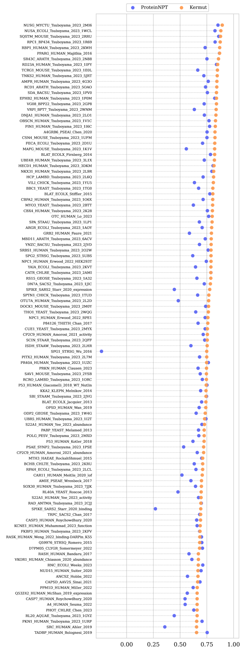
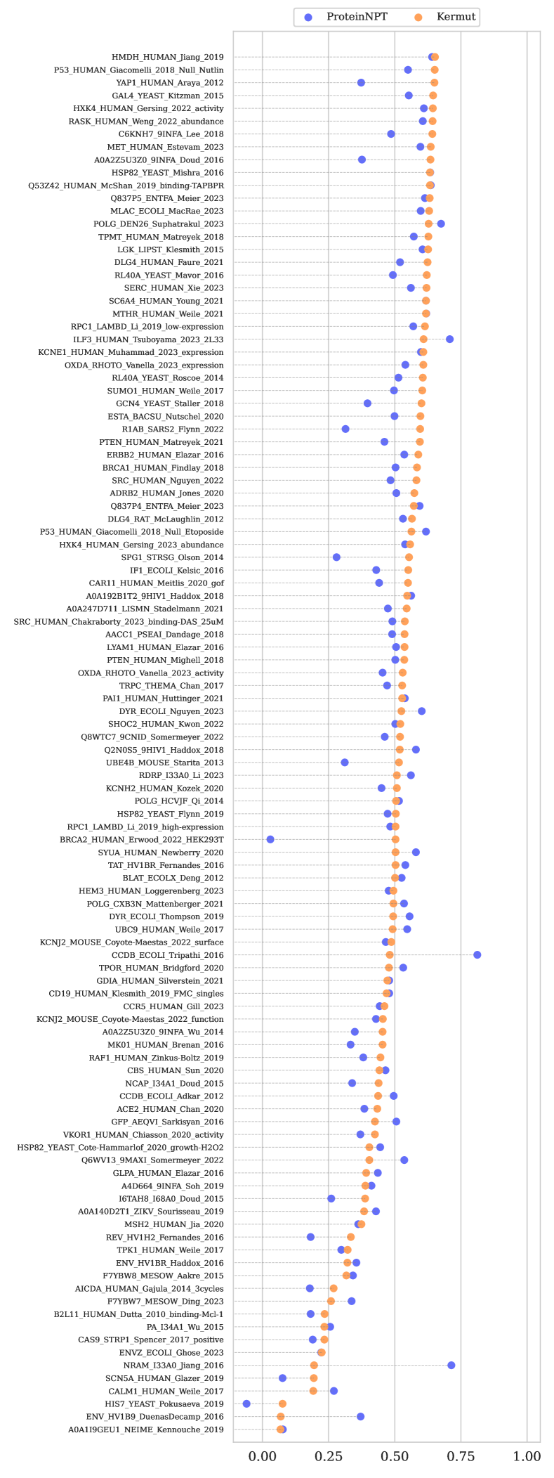
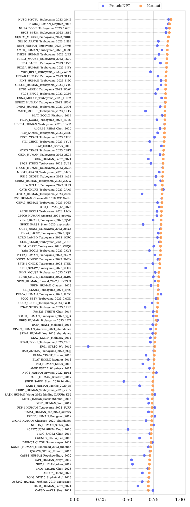
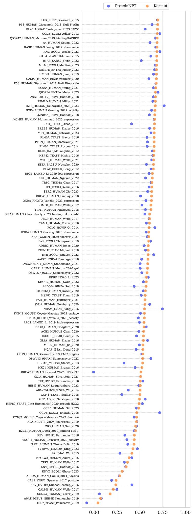
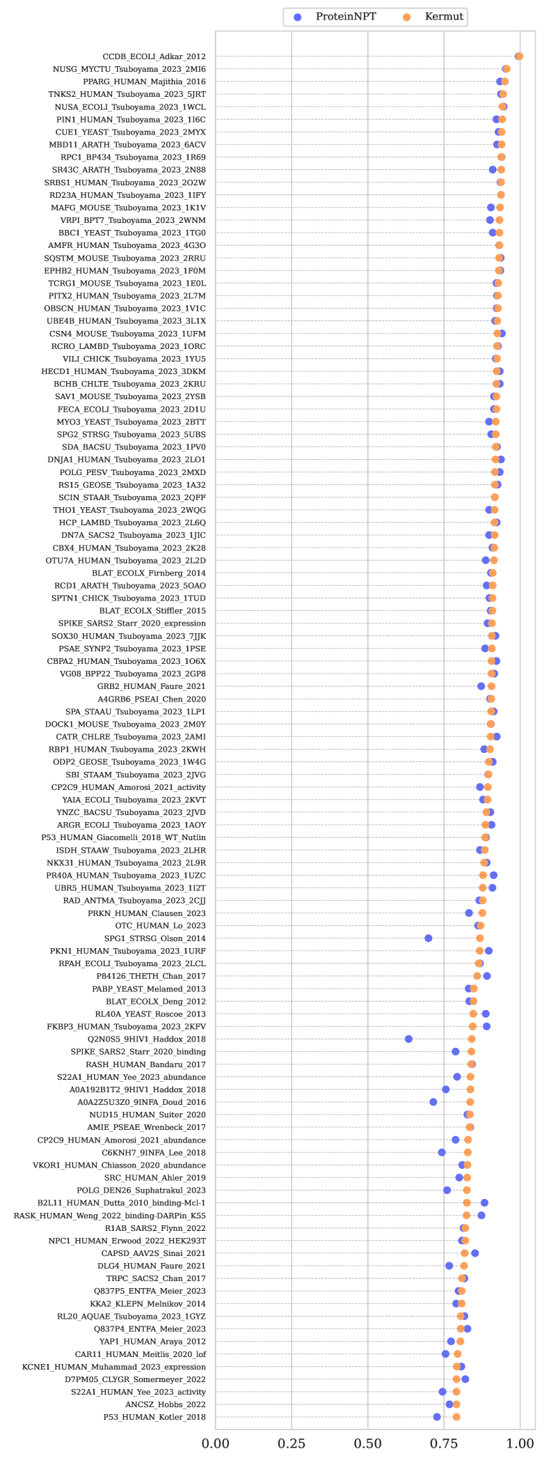
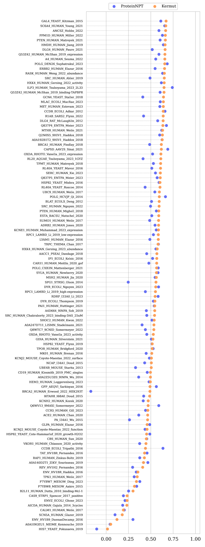
The non-parametric bootstrap standard error for each model relative to Kermut can be seen in Tables 5 and 7. In Appendix L, we provide additional results using alternate zero-shot functions. We also include the performance per functional category, showing similar results (Appendix E). The average and per-split performance for individual assays can be seen in Figures 16, 17, 18 and 19 while additional details on computation time can be seen in Section B.3.
4.1 Ablation study
To examine the impact of Kermut’s components, we conduct an ablation study, where we ablate its two main kernels from Equation 4 – the structure and sequence kernels – as well as the structure kernel’s subcomponents. We similarly investigate the importance of the zero-shot mean function. The ablation study is carried out on all split schemes on a subset of 174 datasets. The difference between the ablation results and the Kermut results can be seen in Table 2, where larger values indicate large component importance. For the absolute values, see Appendix F.
As indicated by the largest drop in performance, the single most important component is the structure kernel. While removing the sequence kernel leads to comparable decreases for all three schemes, removing the structure kernel primarily leads to drops in the challenging contiguous and modulo schemes. This shows that the structure kernel is crucial for characterizing unseen sites in the wild type protein. While removing the site comparison and mutation probability kernels leads to small and medium drops in performance, we observe that removing both leads to an even larger performance drop, indicating an interplay between the two. We lastly see that the inclusion of a zero-shot mean function provides a decent performance increase.
4.2 Uncertainty quantification per mutation domain
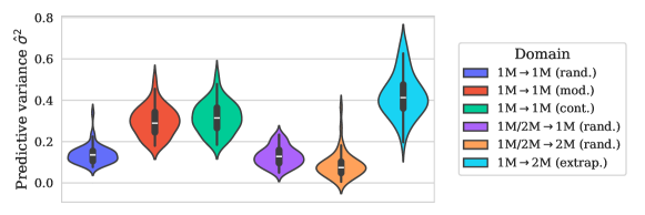
By inspecting the posterior predictive variance, we can analyze model uncertainty. To this end, we define several mutation domains of interest [34]. We designate the three split schemes from the ProteinGym benchmark as three such domains. These are examples of interpolation, where we both train and test on single mutants (1M1M). While the main benchmark only considers single mutations, some assays include additional variants with multiple mutations. We consider a number of these and define two additional interpolation domains where we train on both single and double mutations (1M/2M) and test on singles and doubles, respectively. As a challenging sixth domain, we train on single mutations only and test on doubles (1M2M), constituting an extrapolation domain. For details on the multi-mutant splits, see Appendix G.
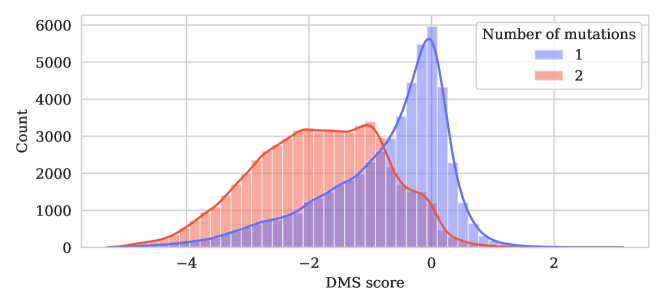
Figure 2 shows the distributions of mean predictive variances in the six domains. In the three single mutant domains, we observe that the uncertainties increase from scheme to scheme, reflecting the difficulties of the tasks and analogously the expected performance scores (Table 1). Suprisingly, when training on both single and double mutants (1M/2M), we observe a lower uncertainty on double mutants than single mutants. For many of the multi-mutant datasets, the mutants are not uniformly sampled but often include a fixed single mutation. A possible explanation is thus that it might be more challenging to decouple the signal from a double mutation into its constituent single mutation signals. In the extrapolation setting, we observe large predictive uncertainties, as expected. One explanation of the discrepancy between the variance distributions in the multi-mutant domains might lie in the difference in target distributions between training and test sets. Figure 4 in the appendix shows the overall target distribution of assays for the 51 considered multi-mutant datasets. The single and double mutants generally belong to different modalities, where the double mutants often lead to a loss of fitness. This shows the difficulty of predicting on domains not encountered during training. For reference, we include the results for the multi-mutant domains in Table 12 in the appendix.
| Uniprot ID | Spearman () | Details | ||||||
|---|---|---|---|---|---|---|---|---|
| Contig. | Mod. | Rand. | Avg. | Assay | Source | |||
| BLAT_ECOLX | 0.825 | 0.832 | 0.907 | 0.855 | 4996 | 286 | Organismal fitness | [36] |
| PA_I34A1 | 0.322 | 0.485 | 0.542 | 0.450 | 1820 | 716 | Organismal fitness | [37] |
| TCRG1_MOUSE | 0.660 | 0.637 | 0.891 | 0.729 | 621 | 37 | Stability | [4] |
| OPSD_HUMAN | 0.653 | 0.699 | 0.866 | 0.691 | 165 | 348 | Expression | [38] |
4.3 Uncertainty calibration analysis
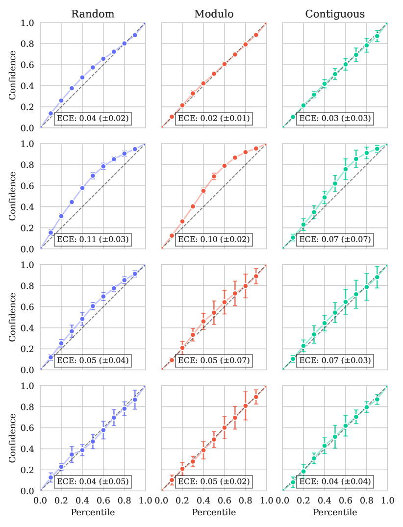
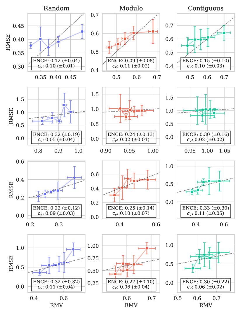
To clarify the relationship between model uncertainty and expected performance, we proceed with a calibration analysis. First, we perform a confidence interval-based calibration analysis [39], resulting in calibration curves which in the classification setting are known as reliability diagrams [40]. The results for each dataset are obtained via five-fold cross validation, corresponding to five separately trained models for each split scheme. We select four diverse datasets as examples (Table 3), reflecting both high and low predictive performance. The mean calibration curves can be seen in Figure 3(a). For method details and results across all datasets, see Appendix I. The mean expected calibration error (ECE) is shown in the bottom of each plot, where a value of zero indicates perfect calibration. Overall, the uncertainties appear to be well-calibrated both qualitatively from the curves and quantitatively from the ECEs. Even the smallest dataset (fourth row, ) achieves decent calibration, albeit with larger variances between folds.
While the confidence interval-based calibration curves show that we can trust the uncertainty estimates overall, they do not indicate whether we can trust individual predictions. We therefore supplement the above analysis with an error-based calibration analysis [41], where a well-calibrated model will have low uncertainty when the error is low. The calibration curves can be seen in Figure 3(b). We compute the per CV-fold expected normalized calibration error (ENCE) and the coefficient of variation (), which quantifies the variance of the predicted uncertainties. Ideally, the ENCE should be zero while the coefficient of variation should be relatively large (indicating spread-out uncertainties).
While the confidence interval-based analysis suggested that the uncertainty estimates were well-calibrated with some under-confidence, the same is not as visibly clear for the error-based calibration plots. We do however see a trend of increasing error with increasing uncertainty in three of the four datasets, where the curves lie close to the diagonal (as indicated by the dashed line). The second row shows poorer calibration – particularly in the modulo and contiguous schemes. The curves however remain difficult to interpret, in part due to the errorbars on both axes. To alleviate this, we compute similar metrics for all 217 datasets across the three splits, which indicate that, though varying, most calibration curves are well-behaved (see Section I.3).
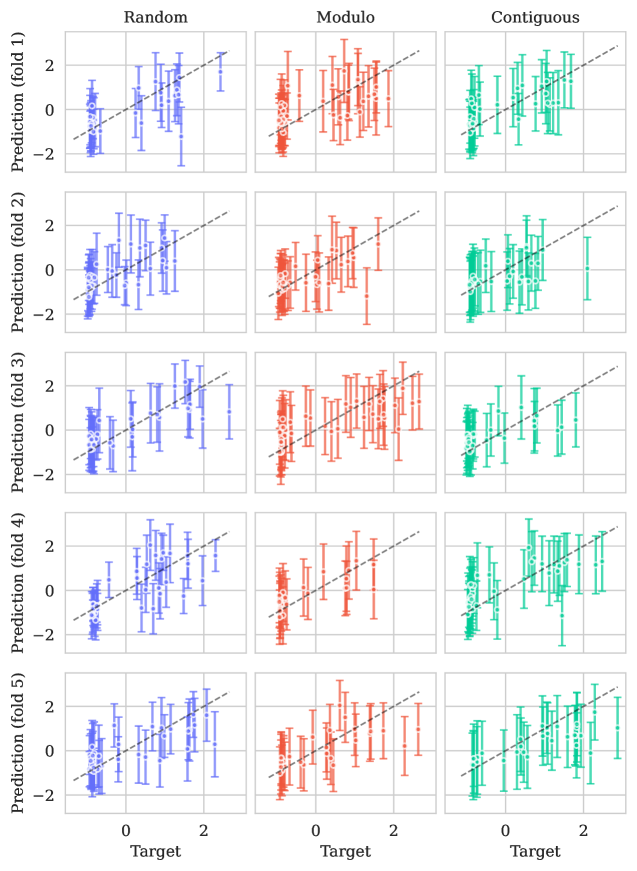
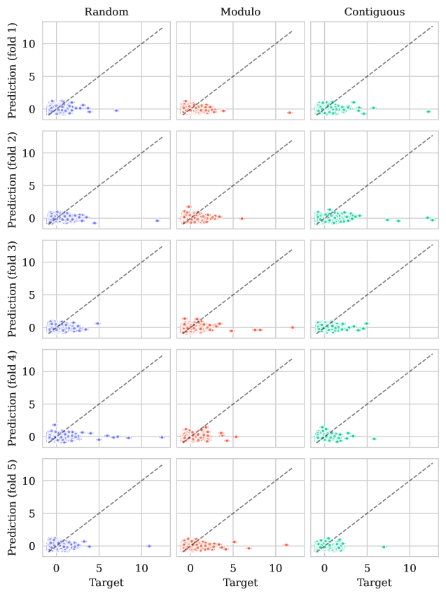
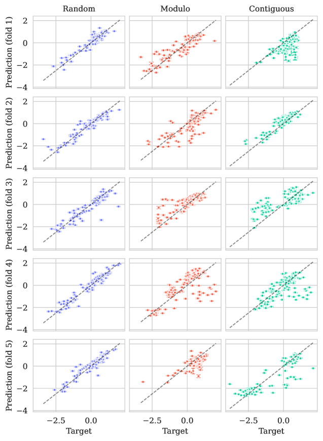
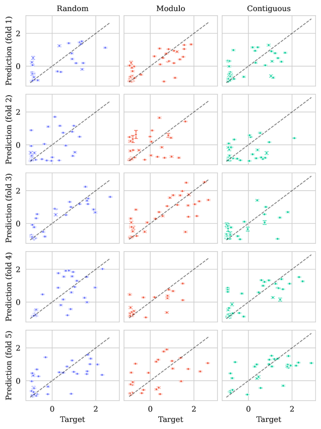
We supplement the above calibration curves with Figures 7, 8, 9 and 10 in the Appendix, which show the true values plotted against the predictions. These highlight the importance of well-calibrated uncertainties and underline their role in interpreting model predictions and their trustworthiness.
4.3.1 Comparison with ProteinNPT
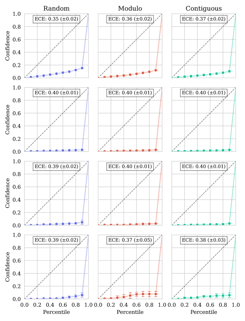
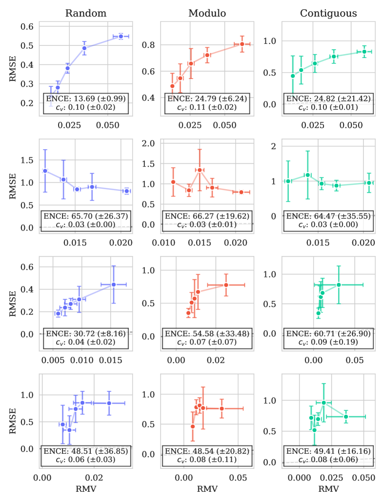
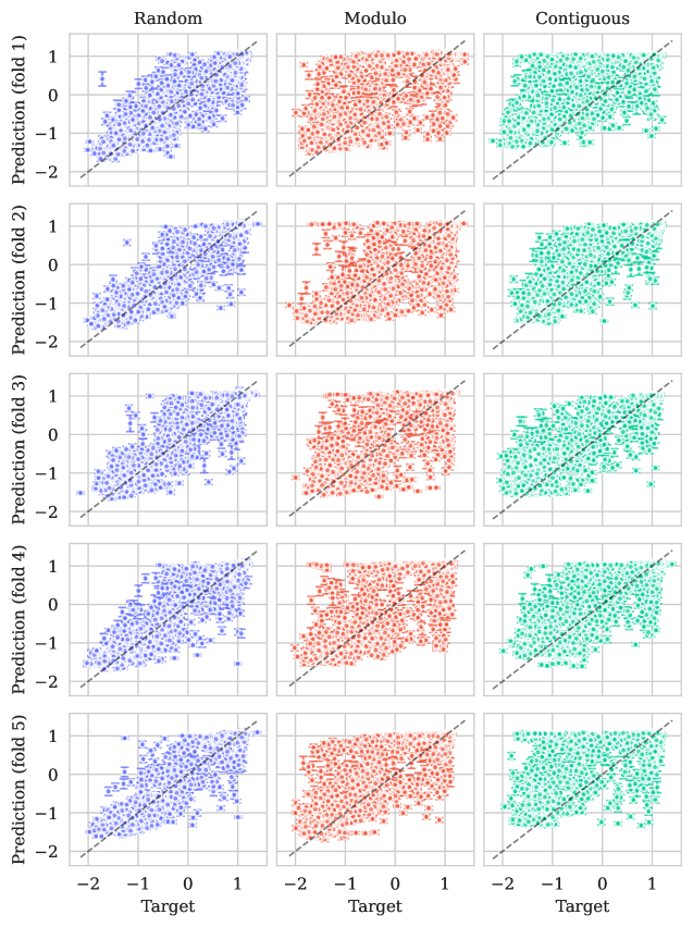
Monte Carlo (MC) dropout [42] is a popular uncertainty quantification technique for deep learning models. Calibration curves for ProteinNPT with MC dropout for the same four datasets across the three split schemes can be seen in Figure 11 while figures showing the true values plotted against the predictions with uncertainties are shown in Section K.3. These indicate that employing MC dropout on a deep learning model like ProteinNPT seems to provide lower levels of calibration, providing overconfident uncertainties across assays and splits. Due to the generally low uncertainties and the resulting difference in scales, the calibration curves are often far from the diagonal. The trends in the calibration curves however show that the model errors often correlate with the uncertainties. This suggests that the model can be recalibrated to achieve decent calibration.
Other techniques for uncertain quantification in deep learning models certainly exist, and we by no means rule out that other techniques can outperform our method (see Discussion below). We note, however, that many uncertainty quantification methods will be associated with considerable computational overhead compared to the built-in capabilities of a Gaussian process.
5 Discussion
We have shown that a carefully constructed Gaussian process is able to reach state-of-the-art performance for protein variant effect prediction while providing reasonably well-calibrated uncertainty estimates. For a majority of datasets, this is achieved orders of magnitude faster than competing methods.
While the predictive performance on the substitution benchmark is an improvement over previous methods, our proposed model has its limitations. Due to the site-comparison mechanism, our model is unable to handle insertions and deletions as it only operates on a fixed structure. Additionally, as the number of mutations increases, the assumption of a fixed structure might worsen, depending on the introduced mutations, which can affect reliability. While this limitation can be fixed by online protein structure prediction, the computational cost would increase significantly. This however applies to all structure-based methods in the context of introducing large numbers of mutations and is thus not particular to Kermut. An additional limitation is the GP’s scaling with dataset size. While not a major obstacle in the single mutant setting, dataset sizes can quickly grow when handling multiple mutants. The last decades have however produced a substantial literature on algorithms for scaling GPs to larger datasets [43, 44, 45], which could alleviate the issue, and we therefore believe this to be a technical, rather than fundamental limitation.
Well-calibrated uncertainties are crucial for protein engineering; both when relying on a Bayesian optimization routine to guide experimental design using uncertainty-dependent acquisition functions and similarly to weigh the risk versus reward for experimentally synthesizing suggested variants. We therefore encourage the community to place a greater emphasis on uncertainty quantification and calibration for protein prediction models as this will have measurable impacts in real-life applications like protein engineering – perhaps more so than increased prediction accuracy. We hope that Kermut can serve as a fruitful step in this direction.
Acknowledgments and Disclosure of Funding
This work was funded in part by Innovation Fund Denmark (1044-00158A), the Novo Nordisk Synergy grant (NNF200C0063709), the Novo Nordisk Foundation through the MLSS Center (Basic Machine Learning Research in Life Science, NNF20OC0062606), and the Pioneer Centre for AI (DNRF grant number P1).
References
- [1] Adam J. Riesselman, John B. Ingraham, and Debora S. Marks. Deep generative models of genetic variation capture the effects of mutations. Nature Methods, 15(10):816–822, October 2018.
- [2] Alexander Rives, Joshua Meier, Tom Sercu, Siddharth Goyal, Zeming Lin, Jason Liu, Demi Guo, Myle Ott, C. Lawrence Zitnick, Jerry Ma, and Rob Fergus. Biological structure and function emerge from scaling unsupervised learning to 250 million protein sequences, December 2020.
- [3] Jun Cheng, Guido Novati, Joshua Pan, Clare Bycroft, Akvilė Žemgulytė, Taylor Applebaum, Alexander Pritzel, Lai Hong Wong, Michal Zielinski, Tobias Sargeant, Rosalia G. Schneider, Andrew W. Senior, John Jumper, Demis Hassabis, Pushmeet Kohli, and Žiga Avsec. Accurate proteome-wide missense variant effect prediction with AlphaMissense. Science, 381(6664):eadg7492, September 2023.
- [4] Kotaro Tsuboyama, Justas Dauparas, Jonathan Chen, Elodie Laine, Yasser Mohseni Behbahani, Jonathan J. Weinstein, Niall M. Mangan, Sergey Ovchinnikov, and Gabriel J. Rocklin. Mega-scale experimental analysis of protein folding stability in biology and design. Nature, pages 1–11, July 2023.
- [5] Christian Dallago, Jody Mou, Kadina E. Johnston, Bruce J. Wittmann, Nicholas Bhattacharya, Samuel Goldman, Ali Madani, and Kevin K. Yang. FLIP: Benchmark tasks in fitness landscape inference for proteins, January 2022.
- [6] Pascal Notin, Aaron W. Kollasch, Daniel Ritter, Lood Van Niekerk, Steffan Paul, Han Spinner, Nathan J. Rollins, Ada Shaw, Rose Orenbuch, Ruben Weitzman, Jonathan Frazer, Mafalda Dias, Dinko Franceschi, Yarin Gal, and Debora Susan Marks. ProteinGym: Large-Scale Benchmarks for Protein Fitness Prediction and Design. In Thirty-Seventh Conference on Neural Information Processing Systems Datasets and Benchmarks Track, November 2023.
- [7] Jonathan Foldager, Mikkel Jordahn, Lars Kai Hansen, and Michael Riis Andersen. On the role of model uncertainties in bayesian optimization. In Proceedings of the Thirty-Ninth Conference on Uncertainty in Artificial Intelligence, UAI ’23. JMLR.org, 2023.
- [8] Jonathan Frazer, Pascal Notin, Mafalda Dias, Aidan Gomez, Joseph K. Min, Kelly Brock, Yarin Gal, and Debora S. Marks. Disease variant prediction with deep generative models of evolutionary data. Nature, 599(7883):91–95, November 2021.
- [9] Joshua Meier, Roshan Rao, Robert Verkuil, Jason Liu, Tom Sercu, and Alexander Rives. Language models enable zero-shot prediction of the effects of mutations on protein function, July 2021.
- [10] Pascal Notin, Mafalda Dias, Jonathan Frazer, Javier Marchena-Hurtado, Aidan Gomez, Debora S. Marks, and Yarin Gal. Tranception: Protein fitness prediction with autoregressive transformers and inference-time retrieval, May 2022.
- [11] Kevin K. Yang, Zachary Wu, and Frances H. Arnold. Machine-learning-guided directed evolution for protein engineering. Nature Methods, 16(8):687–694, August 2019.
- [12] Zeming Lin, Halil Akin, Roshan Rao, Brian Hie, Zhongkai Zhu, Wenting Lu, Allan dos Santos Costa, Maryam Fazel-Zarandi, Tom Sercu, Sal Candido, and Alexander Rives. Language models of protein sequences at the scale of evolution enable accurate structure prediction. Preprint, Synthetic Biology, July 2022.
- [13] Ahmed Elnaggar, Michael Heinzinger, Christian Dallago, Ghalia Rehawi, Yu Wang, Llion Jones, Tom Gibbs, Tamas Feher, Christoph Angerer, Martin Steinegger, Debsindhu Bhowmik, and Burkhard Rost. ProtTrans: Towards Cracking the Language of Life’s Code Through Self-Supervised Learning, May 2021.
- [14] Chloe Hsu, Hunter Nisonoff, Clara Fannjiang, and Jennifer Listgarten. Learning protein fitness models from evolutionary and assay-labeled data. Nature Biotechnology, pages 1–9, January 2022.
- [15] Pascal Notin, Ruben Weitzman, Debora Marks, and Yarin Gal. ProteinNPT: Improving Protein Property Prediction and Design with Non-Parametric Transformers. In A. Oh, T. Neumann, A. Globerson, K. Saenko, M. Hardt, and S. Levine, editors, Advances in Neural Information Processing Systems, volume 36, pages 33529–33563. Curran Associates, Inc., 2023.
- [16] Roshan M. Rao, Jason Liu, Robert Verkuil, Joshua Meier, John Canny, Pieter Abbeel, Tom Sercu, and Alexander Rives. MSA Transformer. In Proceedings of the 38th International Conference on Machine Learning, pages 8844–8856. PMLR, July 2021.
- [17] Roshan Rao, Nicholas Bhattacharya, Neil Thomas, Yan Duan, Xi Chen, John Canny, Pieter Abbeel, and Yun S. Song. Evaluating Protein Transfer Learning with TAPE. arXiv:1906.08230 [cs, q-bio, stat], June 2019.
- [18] Minghao Xu, Zuobai Zhang, Jiarui Lu, Zhaocheng Zhu, Yangtian Zhang, Chang Ma, Runcheng Liu, and Jian Tang. PEER: A Comprehensive and Multi-Task Benchmark for Protein Sequence Understanding, June 2022.
- [19] Raphael J. L. Townshend, Martin Vögele, Patricia Suriana, Alexander Derry, Alexander Powers, Yianni Laloudakis, Sidhika Balachandar, Bowen Jing, Brandon Anderson, Stephan Eismann, Risi Kondor, Russ B. Altman, and Ron O. Dror. ATOM3D: Tasks On Molecules in Three Dimensions. arXiv:2012.04035 [physics, q-bio], January 2022.
- [20] Peter Mørch Groth, Richard Michael, Jesper Salomon, Pengfei Tian, and Wouter Boomsma. FLOP: Tasks for Fitness Landscapes Of Protein wildtypes, June 2023.
- [21] Christina Leslie, Eleazar Eskin, and William Stafford Noble. The spectrum kernel: A string kernel for svm protein classification. In Biocomputing 2002, pages 564–575. WORLD SCIENTIFIC, December 2001.
- [22] Christina S. Leslie, Eleazar Eskin, Adiel Cohen, Jason Weston, and William Stafford Noble. Mismatch string kernels for discriminative protein classification. Bioinformatics, 20(4):467–476, March 2004.
- [23] Philip A. Romero, Andreas Krause, and Frances H. Arnold. Navigating the protein fitness landscape with Gaussian processes. Proceedings of the National Academy of Sciences, 110(3):E193–E201, January 2013.
- [24] Emmi Jokinen, Markus Heinonen, and Harri Lähdesmäki. mGPfusion: Predicting protein stability changes with Gaussian process kernel learning and data fusion. Bioinformatics, 34(13):i274–i283, July 2018.
- [25] John Ingraham, Vikas K. Garg, Regina Barzilay, and Tommi Jaakkola. Generative models for graph-based protein design. Curran Associates Inc., Red Hook, NY, USA, 2019.
- [26] Chloe Hsu, Robert Verkuil, Jason Liu, Zeming Lin, Brian Hie, Tom Sercu, Adam Lerer, and Alexander Rives. Learning inverse folding from millions of predicted structures. In Proceedings of the 39th International Conference on Machine Learning, pages 8946–8970. PMLR, June 2022.
- [27] J. Dauparas, I. Anishchenko, N. Bennett, H. Bai, R. J. Ragotte, L. F. Milles, B. I. M. Wicky, A. Courbet, R. J. de Haas, N. Bethel, P. J. Y. Leung, T. F. Huddy, S. Pellock, D. Tischer, F. Chan, B. Koepnick, H. Nguyen, A. Kang, B. Sankaran, A. K. Bera, N. P. King, and D. Baker. Robust deep learning based protein sequence design using ProteinMPNN, June 2022.
- [28] Zhangyang Gao, Cheng Tan, Pablo Chacón, and Stan Z. Li. PiFold: Toward effective and efficient protein inverse folding, April 2023.
- [29] David Ding, Ada Y. Shaw, Sam Sinai, Nathan Rollins, Noam Prywes, David F. Savage, Michael T. Laub, and Debora S. Marks. Protein design using structure-based residue preferences. Nature Communications, 15(1):1639, February 2024.
- [30] P. Gainza, F. Sverrisson, F. Monti, E. Rodolà, D. Boscaini, M. M. Bronstein, and B. E. Correia. Deciphering interaction fingerprints from protein molecular surfaces using geometric deep learning. Nature Methods, 17(2):184–192, February 2020.
- [31] Pablo Gainza, Sarah Wehrle, Alexandra Van Hall-Beauvais, Anthony Marchand, Andreas Scheck, Zander Harteveld, Stephen Buckley, Dongchun Ni, Shuguang Tan, Freyr Sverrisson, Casper Goverde, Priscilla Turelli, Charlène Raclot, Alexandra Teslenko, Martin Pacesa, Stéphane Rosset, Sandrine Georgeon, Jane Marsden, Aaron Petruzzella, Kefang Liu, Zepeng Xu, Yan Chai, Pu Han, George F. Gao, Elisa Oricchio, Beat Fierz, Didier Trono, Henning Stahlberg, Michael Bronstein, and Bruno E. Correia. De novo design of protein interactions with learned surface fingerprints. Nature, 617(7959):176–184, May 2023.
- [32] John Jumper, Richard Evans, Alexander Pritzel, Tim Green, Michael Figurnov, Olaf Ronneberger, Kathryn Tunyasuvunakool, Russ Bates, Augustin Žídek, Anna Potapenko, Alex Bridgland, Clemens Meyer, Simon A. A. Kohl, Andrew J. Ballard, Andrew Cowie, Bernardino Romera-Paredes, Stanislav Nikolov, Rishub Jain, Jonas Adler, Trevor Back, Stig Petersen, David Reiman, Ellen Clancy, Michal Zielinski, Martin Steinegger, Michalina Pacholska, Tamas Berghammer, Sebastian Bodenstein, David Silver, Oriol Vinyals, Andrew W. Senior, Koray Kavukcuoglu, Pushmeet Kohli, and Demis Hassabis. Highly accurate protein structure prediction with AlphaFold. Nature, 596(7873):583–589, August 2021.
- [33] Carl Edward Rasmussen and Christopher K. I. Williams. Gaussian Processes for Machine Learning. Adaptive Computation and Machine Learning. MIT Press, Cambridge, Mass, 2006.
- [34] Richard Michael, Jacob Kæstel-Hansen, Peter Mørch Groth, Simon Bartels, Jesper Salomon, Pengfei Tian, Nikos S. Hatzakis, and Wouter Boomsma. A systematic analysis of regression models for protein engineering. PLOS Computational Biology, 20(5):e1012061, May 2024.
- [35] Richard Michael, Simon Bartels, Miguel González-Duque, Yevgen Zainchkovskyy, Jes Frellsen, Søren Hauberg, and Wouter Boomsma. A Continuous Relaxation for Discrete Bayesian Optimization, April 2024.
- [36] Michael A. Stiffler, Doeke R. Hekstra, and Rama Ranganathan. Evolvability as a Function of Purifying Selection in TEM-1 -Lactamase. Cell, 160(5):882–892, February 2015.
- [37] Nicholas C. Wu, C. Anders Olson, Yushen Du, Shuai Le, Kevin Tran, Roland Remenyi, Danyang Gong, Laith Q. Al-Mawsawi, Hangfei Qi, Ting-Ting Wu, and Ren Sun. Functional Constraint Profiling of a Viral Protein Reveals Discordance of Evolutionary Conservation and Functionality. PLOS Genetics, 11(7):e1005310, July 2015.
- [38] Aliete Wan, Emily Place, Eric A. Pierce, and Jason Comander. Characterizing variants of unknown significance in rhodopsin: A functional genomics approach. Human Mutation, 40(8):1127–1144, August 2019.
- [39] Gabriele Scalia, Colin A. Grambow, Barbara Pernici, Yi-Pei Li, and William H. Green. Evaluating Scalable Uncertainty Estimation Methods for Deep Learning-Based Molecular Property Prediction. ACS, 2020.
- [40] Morris H. DeGroot and Stephen E. Fienberg. The comparison and evaluation of forecasters. Journal of the Royal Statistical Society. Series D (The Statistician), 32(1/2):12–22, 1983.
- [41] Dan Levi, Liran Gispan, Niv Giladi, and Ethan Fetaya. Evaluating and Calibrating Uncertainty Prediction in Regression Tasks, February 2020.
- [42] Yarin Gal and Zoubin Ghahramani. Dropout as a bayesian approximation: Representing model uncertainty in deep learning. In Maria Florina Balcan and Kilian Q. Weinberger, editors, Proceedings of The 33rd International Conference on Machine Learning, volume 48 of Proceedings of Machine Learning Research, pages 1050–1059, New York, New York, USA, 20–22 Jun 2016. PMLR.
- [43] Edward Snelson and Zoubin Ghahramani. Sparse gaussian processes using pseudo-inputs. In Proceedings of the 18th International Conference on Neural Information Processing Systems, NIPS’05, page 1257–1264, Cambridge, MA, USA, 2005. MIT Press.
- [44] Ke Alexander Wang, Geoff Pleiss, Jacob R. Gardner, Stephen Tyree, Kilian Q. Weinberger, and Andrew Gordon Wilson. Exact Gaussian Processes on a Million Data Points, December 2019. arXiv:1903.08114 [cs, stat].
- [45] Giacomo Meanti, Luigi Carratino, Lorenzo Rosasco, and Alessandro Rudi. Kernel methods through the roof: Handling billions of points efficiently. In H. Larochelle, M. Ranzato, R. Hadsell, M.F. Balcan, and H. Lin, editors, Advances in Neural Information Processing Systems, volume 33, pages 14410–14422. Curran Associates, Inc., 2020.
- [46] I. Csiszár and P.C. Shields. Information theory and statistics: A tutorial. Foundations and Trends® in Communications and Information Theory, 1(4):417–528, 2004.
- [47] Nicki Skafte Detlefsen, Søren Hauberg, and Wouter Boomsma. Learning meaningful representations of protein sequences. Nature Communications, 13(1):1914, April 2022.
- [48] Thomas Gärtner, Peter A. Flach, Adam Kowalczyk, and Alex J. Smola. Multi-instance kernels. In Proceedings of the Nineteenth International Conference on Machine Learning, ICML ’02, page 179–186, San Francisco, CA, USA, 2002. Morgan Kaufmann Publishers Inc.
- [49] Jacob R. Gardner, Geoff Pleiss, David Bindel, Kilian Q. Weinberger, and Andrew Gordon Wilson. GPyTorch: Blackbox Matrix-Matrix Gaussian Process Inference with GPU Acceleration, June 2021.
- [50] Nicholas G. Polson and James G. Scott. On the half-Cauchy prior for a global scale parameter, September 2011.
- [51] Ilya Loshchilov and Frank Hutter. Decoupled Weight Decay Regularization, January 2019.
Appendix
Appendix A GP details
A.1 Structure kernel
The structure kernel is comprised of three components, each increasing model flexibility. The site-comparison kernel, , compares site-specific, structure-conditioned amino acid distributions. Given two such discrete probability distributions, and , their distance is quantified via the Hellinger distance [46]
which is used in the Hellinger kernel [35]
For the mutation probability kernel, , we use the log-probabilities rather than the amino acid identities to reflect that amino acids with similar probability on sites with similar distributions should have similar biochemical effects on the protein. We do not include the log-probabilities of the wild type amino acids, as the inverse folding model by definition is trained to assign high probabilities to the wild type sequence. The exact probability of a wild type amino acid depends on how many other amino acids that are likely to be at the given site. For example, we would expect a probability close to one for a functionally critical amino acid at a particular site. Conversely, for a less critical surface-level residue requiring, e.g., a polar uncharged amino acid, we would expect similar probabilities for the four amino acids of this type. Thus, variations of log-probabilities of the wild type amino acids should be reflected in the distribution on the sites captured by the Hellinger kernel.
For the per-residue amino acid distributions in and , we use ProteinMPNN [27]. ProteinMPNN relies on a random decoding order and thus benefits from multiple samples. We decode the wild type amino acid sequence a total of ten times while conditioning on the full structure and the sequence that has been decoded thus far. We then compute a per-residue average distribution. We use the v_48_020 weights.
A.2 Sequence kernel
For the sequence kernel, we use embeddings extracted from the ESM-2 protein language model [12]. We use the esm2_t36_650M_UR50D model with 650M parameters. The embeddings are mean-pooled across the sequence dimension such that each variant is represented by a 1280 dimensional vector. While it has been shown that other aggregation method can lead to large increases in performance [47], we consider alternate methods such as training a bottleneck model out of the scope of this paper.
A.3 Parametrization note
An alternative formulation of the kernel, where we omit from Equation 2 and from Equation 4, and instead provide the structure and sequence kernels with separate coefficients have shown to provide close to identical results when using a smoothed box prior (constrained between 0 and 1). While this approach is somewhat more elegant, this does not justify the re-computation of all results.
A.4 Zero-shot mean function
For the zero-shot mean function, we download and use the pre-computed zero-shot scores from ProteinGym at https://github.com/OATML-Markslab/ProteinGym. The zero-shot value is calculated as the log-likelihood ratio between the variant and the wild type at the mutated residue as described in [9]:
The values can be computed straightforwardly using the ESM suite (using the masked-marginals strategy). For multi-mutants, the sum of the ratios is taken.
A.5 Kernel proof
We will in the following argue why Kermut’s structure kernel is a valid kernel. Recall that a function is a kernel if and only if the matrix , where , is symmetric positive semi-definite [33]. From literature we know a number of kernels and certain ways these can be combined to create new kernels. We will argue that Kermut is a kernel by showing how it is composed of known kernels, combined using valid methods.
Note that, if we have a mapping and a kernel , on , then defined by is a kernel on .
Let be the space of sequences parameterized with respect to a reference sequence. Let be a transformation of the sequences defined as in Section 3.3. is the squared exponential kernel on the transformed variants. Hence, is is a kernel on .
Let denote the subspace of single mutant variants and be a function mapping single mutant variants into the 3D coordinates of the -carbon of the particular mutation. is the exponential kernel on this transformed space. Thus is a kernel on .
Let be defined as in Section 3.3, where is the space of probability distributions over the 20 amino acids. is the probability distribution over the mutated site of given by an inverse folding model. is the Hellinger kernel on the single mutation variants transformed by , hence, a valid kernel on . Likewise is the exponential kernel of a transformation, as defined in Section 3.3, of the sequences, hence also a kernel.
Scaling, multiplying, and adding kernels result in new kernels, making a valid kernel for single mutations [33]. We need to show that and thereby is valid for any number of mutations.
Let be a function taking a variant with mutations and mapping it to a set of all the single mutations which constitutes . Define the set kernel [48]
is the set kernel on the transformed input and thus also a kernel. We have thereby shown that Kermut is a kernel for variants with any number of mutations.
Appendix B Implementation details
B.1 General details
We build our kernel using the GPyTorch framework [49]. We assume a homoschedastic Gaussian noise model, on which we place a HalfCauchy prior [50] with scale . We fit the hyperparameters by maximizing the exact marginal likelihood with gradient descent using the AdamW optimizer [51] with learning rate 0.1 for a 150 steps, which proved to be sufficient for convergence for a number of sampled datasets. For larger, more complex datasets, alternate learning rates and optimization steps might lead to improved results.
B.2 System details
All experiments are performed on a Linux-based cluster running Ubuntu 20.04.4 LTS, with a AMD EPYC 7642 48-Core Processor with 192 threads and 1TB RAM. NVIDIA A40s were used for GPU acceleration both for fitting the Gaussian processes and for generating the protein embeddings.
B.3 Compute time
There are multiple factors to consider when evaluating the training time of Kermut. A limitation of using a Gaussian process framework is the cubic scaling with dataset size. For this reason, we ran the ablation study on only 174 of the 217 datasets.
Training Kermut on these datasets for a single split-scheme using the aforementioned hardware (single GPU) takes approximately 1 hour and 30 minutes. Getting ablation results for all three schemes thus takes between 4-5 hours. This however assumes that
-
1.
the embeddings for the sequence kernel have been precomputed,
-
2.
the probability distribution for all sites in the wild type protein have been precomputed,
-
3.
and that the zero-shot scores have been precomputed.
We do not see any of these as major limitations as the same applies to ProteinNPT and similar models.
Scaling the experiments to the full ProteinGym benchmark is however costly. We were able to train/evaluate Kermut on 205/217 datasets using an NVIDIA A40 GPU with 48GB VRAM. The remaining 12 datasets were too large to fit into GPU memory without resorting to reduced precision. For these, we trained and evaluated the model using CPU only which takes considerable time. These datasets are
-
•
HMDH_HUMAN_Jiang_2019
-
•
HSP82_YEAST_Flynn_2019
-
•
MSH2_HUMAN_Jia_2020
-
•
MTHR_HUMAN_Weile_2021
-
•
POLG_CXB3N_Mattenberger_2021
-
•
POLG_DEN26_Suphatrakul_2023
-
•
Q2N0S5_9HIV1_Haddox_2018
-
•
RDRP_I33A0_Li_2023
-
•
S22A1_HUMAN_Yee_2023_abundance
-
•
S22A1_HUMAN_Yee_2023_activity
-
•
SC6A4_HUMAN_Young_2021
-
•
SHOC2_HUMAN_Kwon_2022
B.3.1 Example wall-clock time
The wall-clock times for generating the results used for the calibration curves in Figures 3(b), 3(a) and 11 for one split scheme can be seen in Table 4 for Kermut and ProteinNPT. The experiments were carried out using identical hardware. The test system is however a shared compute cluster with sharded GPUs, so variance is expected between runs. Generating the full results for the figures thus takes Kermut approximately 10 minutes while ProteinNPT takes 400 hours. This shows the significant reduction in computational burden that Kermut allows for. Both ProteinNPT and Kermut assumes that sequence embeddings are available a priori.
| Dataset | Kermut runtime | PNPT runtime | ||
|---|---|---|---|---|
| BLAT_ECOLX | 111s | h | 4996 | 286 |
| PA_I34A1 | s | h | 1820 | 716 |
| TCRG1_MOUSE | s | h | 621 | 37 |
| OPSD_HUMAN | s | h | 165 | 348 |
Appendix C Data
All data and evaluation software is accessed via the ProteinGym [6] repository at https://github.com/OATML-Markslab/ProteinGym which is under the MIT License.
Appendix D Long sequences
The structures used for obtaining the site-wise probability distributions are predicted by AlphaFold2 [32] and are provided in the ProteinGym repository [6]. The provided structures for A0A140D2T1_ZIKV and POLG_HCVJF do not contain the full structures however, but only a localized area where the mutations occur due to the long sequence lengths. Since our model only operates on sites with mutations, this is not an issue for neither the inverse-folding probability distributions nor the inter-residue distances.
For BRCA2_HUMAN, three PDB files are provided due to the long wild type sequence length. We use ProteinMPNN to obtain the distributions at all sites in each PDB file and stitch them together in a preprocessing step. Calculating the inter-residue distances is however non-trivial and would require a careful alignment of the three structures. Instead, we drop the distance term, , in the kernel for the BRCA2_HUMAN_Erwood_2022_HEK293T dataset (equivalently setting it to one: ).
The sequence kernel operates on ESM-2 embeddings. The ESM-2 model has a maximum sequence length of 1022 amino acids. Protein sequences that are longer than this limit are truncated.
Appendix E Detailed results
The ProteinGym suite provides an aggregation procedure, whereby the predictive performance across both cross-validation schemes and functional categories can be gauged. We provide these results in Tables 5, 6, 7 and 8.
| Model name | Spearman per scheme () | Std. err. | |||
|---|---|---|---|---|---|
| Cont. | Mod. | Rand. | Avg. | ||
| Kermut | 0.611 | 0.634 | 0.747 | 0.664 | 0.000 |
| ProteinNPT | 0.547 | 0.564 | 0.730 | 0.613 | 0.009 |
| Tranception Emb. | 0.490 | 0.526 | 0.696 | 0.571 | 0.007 |
| MSAT Emb. | 0.525 | 0.538 | 0.642 | 0.568 | 0.012 |
| ESM-1v Emb. | 0.481 | 0.506 | 0.639 | 0.542 | 0.011 |
| TranceptEVE + OHE | 0.441 | 0.440 | 0.550 | 0.477 | 0.012 |
| Tranception + OHE | 0.419 | 0.419 | 0.535 | 0.458 | 0.011 |
| MSAT + OHE | 0.410 | 0.412 | 0.536 | 0.453 | 0.014 |
| DeepSequence + OHE | 0.400 | 0.400 | 0.521 | 0.440 | 0.016 |
| ESM-1v + OHE | 0.367 | 0.368 | 0.514 | 0.417 | 0.013 |
| OHE | 0.064 | 0.027 | 0.579 | 0.224 | 0.014 |
| Model name | Spearman per function () | ||||
|---|---|---|---|---|---|
| Activity | Binding | Expression | Fitness | Stability | |
| Kermut | 0.606 | 0.635 | 0.672 | 0.582 | 0.824 |
| ProteinNPT | 0.577 | 0.536 | 0.637 | 0.545 | 0.772 |
| Tranception Emb. | 0.520 | 0.529 | 0.613 | 0.519 | 0.674 |
| MSAT Emb. | 0.547 | 0.470 | 0.584 | 0.493 | 0.749 |
| ESM-1v Emb. | 0.487 | 0.450 | 0.587 | 0.468 | 0.717 |
| TranceptEVE + OHE | 0.502 | 0.444 | 0.476 | 0.470 | 0.493 |
| Tranception + OHE | 0.475 | 0.416 | 0.476 | 0.448 | 0.473 |
| MSAT + OHE | 0.480 | 0.393 | 0.463 | 0.437 | 0.491 |
| DeepSequence + OHE | 0.467 | 0.418 | 0.424 | 0.422 | 0.471 |
| ESM-1v + OHE | 0.421 | 0.363 | 0.452 | 0.383 | 0.463 |
| OHE | 0.213 | 0.212 | 0.226 | 0.194 | 0.273 |
| Model name | MSE per scheme () | Std. err. | |||
|---|---|---|---|---|---|
| Cont. | Mod. | Rand. | Avg. | ||
| Kermut | 0.699 | 0.651 | 0.409 | 0.586 | 0.000 |
| ProteinNPT | 0.820 | 0.771 | 0.459 | 0.683 | 0.018 |
| MSAT Emb. | 0.836 | 0.795 | 0.573 | 0.735 | 0.021 |
| Tranception Emb. | 0.972 | 0.833 | 0.503 | 0.769 | 0.024 |
| ESM-1v Emb. | 0.937 | 0.861 | 0.563 | 0.787 | 0.031 |
| TranceptEVE + OHE | 0.953 | 0.914 | 0.743 | 0.870 | 0.020 |
| MSAT + OHE | 0.963 | 0.934 | 0.749 | 0.882 | 0.021 |
| DeepSequence + OHE | 0.967 | 0.940 | 0.767 | 0.891 | 0.018 |
| Model name | MSE per function () | ||||
|---|---|---|---|---|---|
| Activity | Binding | Expression | Fitness | Stability | |
| Kermut | 0.629 | 0.834 | 0.522 | 0.656 | 0.289 |
| Tranception Emb. | 0.814 | 1.080 | 0.639 | 0.788 | 0.525 |
| ESM-1v Emb. | 0.799 | 1.231 | 0.655 | 0.792 | 0.456 |
| TranceptEVE + OHE | 0.793 | 1.199 | 0.780 | 0.825 | 0.756 |
| MSAT + OHE | 0.810 | 1.221 | 0.788 | 0.836 | 0.756 |
| DeepSequence + OHE | 0.830 | 1.140 | 0.832 | 0.860 | 0.793 |
Appendix F Ablation results
In Section 4.1, an ablation study was carried out by removing components of Kermut. In Table 2, the performance difference in Spearman correlation was shown. In Table 9 we see the performance difference in MSE. The absolute Spearman and MSE values are shown in Tables 10 and 11.
| Description | Ablation | MSE | |||
|---|---|---|---|---|---|
| Contig. | Mod. | Rand. | Avg. | ||
| No structure kernel | |||||
| No sequence kernel | |||||
| No inter-residue dist. | |||||
| No mut. prob./site comp. | |||||
| Const. mean | |||||
| No mut. prob. | |||||
| No site comp. | |||||
| Description | Ablation | Spearman () | |||
|---|---|---|---|---|---|
| Contig. | Mod. | Rand. | Avg. | ||
| No structure kernel | |||||
| No sequence kernel | |||||
| No inter-residue dist. | |||||
| No mut. prob./site comp. | |||||
| Const. mean | |||||
| No mut. prob. | |||||
| No site comp. | |||||
| Kermut | |||||
| Description | Ablation | MSE () | |||
|---|---|---|---|---|---|
| Contig. | Mod. | Rand. | Avg. | ||
| No structure kernel | |||||
| No sequence kernel | |||||
| No inter-residue dist. | |||||
| No mut. prob./site comp. | |||||
| Const. mean | |||||
| No mut. prob. | |||||
| No site comp. | |||||
| Kermut | |||||
Appendix G Results for multi-mutants
69 of the datasets from the ProteinGym benchmark include multi-mutants. In addition to the random, modulo, and contiguous split, these also have a fold_rand_multiples split. We here show the results for Kermut in this setting. Of the 69 datasets, we select 52 which (due to the cubic scaling of fitting GPs) include fewer than 7500 variant sequences. We additionally ignore the GCN4_YEAST_Staller_2018 dataset which has a very large number of mutations. This leads to a total of 51 datasets. All results where the training domain is "1M/2M" are from models trained using the above split. The "1M" domain results correspond to training the model once on single mutants and evaluating it on double mutants. In addition to Kermut, we include as a baseline results from a GP using the sequence kernel operating on mean-pooled ESM-2 embeddings. This is equivalent to setting the structure kernel to 0, as in Table 2.
| Spearman () | MSE () | |||||
|---|---|---|---|---|---|---|
| Domain | Kermut∗ | Kermut | Kermut∗ | Kermut | ||
| 1M/2M1M | 0.856 | 0.904 | 0.910 | 1.701 | 0.156 | 0.140 |
| 1M/2M2M | 0.848 | 0.888 | 0.894 | 1.571 | 0.144 | 0.106 |
| 1M/2M1M/2M | 0.889 | 0.931 | 0.937 | 1.627 | 0.154 | 0.119 |
| 1M2M | 0.647 | 0.660 | 0.650 | 0.505 | 0.583 | 0.804 |
Appendix H Histogram over assays for multi-mutant datasets
A histogram over assay values for 51/69 dataset with multi-mutants can be seen in Figure 4. The histograms are colored according to the number of mutations per variant. The assay distribution belong to different modalities depending on the number of mutations present, where double mutations often lead to a loss of fitness.
Appendix I Uncertainty calibration
I.1 Confidence interval-based calibration
Given a collection of mean predictions and uncertainties, we wish to gauge how well-calibrated the uncertainties are. The posterior predictive mean and variance for each data point is interpreted as a Gaussian distribution and symmetric intervals of varying confidence are placed on each prediction [39]. In a well-calibrated model, approximately x % of predictions should lie within a x % confidence interval, e.g., of observations should fall in the confidence interval. The confidence intervals are discretized into bins and the fraction of predictions falling within in bin is calculated. The calibration curve then plots the confidence intervals vs. the fractions, whereby a diagonal line corresponds to perfect calibration. Given the fractions and confidence intervals, the expected calibration error (ECE) is calculated as
where K is the number of bins, i indicates the equally spaced confidence intervals, and is the fraction of predictions falling within the ith confidence interval.
I.2 Error-based calibration
An alternative method of gauging calibratedness is error-based calibration where the prediction error is tied directly to predictions [39, 41]. The predictions are sorted according to their predictive uncertainty and placed into bins. For each bin, the root mean square error (RMSE) and root mean variance (RMV) is computed. In error-based calibration, a well-calibrated model as equal RMSE and RMV, i.e., a diagonal line. The x and y values in the resulting calibration plot are however not normalized from 0 to 1 as in confidence interval-based calibration. The expected normalized calibration error (ENCE) can be computed as
Additionally, we compute the coefficient of variation () as
where , and where n indexes the N data points [41].
I.3 Uncertainty calibration across all datasets
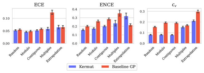
To quantitatively describe the calibratedness of Kermut across all datasets, we compute the above calibration metrics for all split schemes and folds. We do this for Kermut and a baseline GP using the sequence kernel on ESM-2 embeddings (equivalent to the sequence kernel from Equation 1 with a constant mean). These values can be seen in Figure 5 for each of the three main split-schemes, the 1M/2M1M/2M split (“Multiples”), and the 1M2M split (“Extrapolation”). For the three main splits, we see that the calibratedness measured by the ENCE correlates with performance, where the lowest values are seen in the random setting. Generally, we see that the inclusion of the structure kernel improves not only performance (see Table 2) but also calibration, as the ECE and ENCE values are consistently better for Kermut, with the exception of ENCE in the extrapolation domain. We however see that the sequence kernel (squared exponential) consistently provide predictive variances that themselves vary more, which is generally preferable.
Overall, we can conclude that Kermut appears to be well-calibrated both qualitatively and quantitatively. While the ECE values are generally small and similar, the ENCE values suggest a more nuanced calibration landscape, where we can expect low errors when our model predicts low uncertainties, particularly in the random scheme.
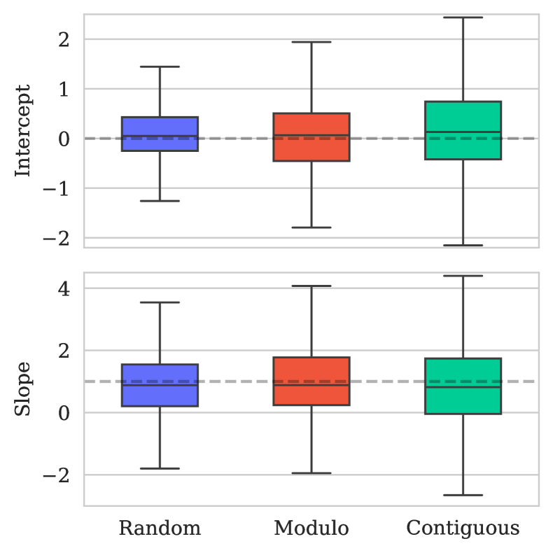
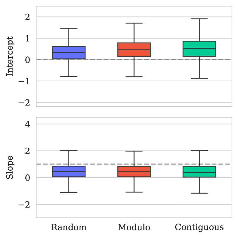
For each dataset, split, and fold, we perform a linear regression to the error-based calibration curves and summarize the slope and intercept. As perfect calibration corresponds to a diagonal line, we want the distribution over the slopes to be centred on one and the distribution over intercepts to be centred on zero. Boxplots for this analysis can be seen in Figure 6. As indicated in (a), most of Kermut’s calibration curves are well-behaved, while the baseline GP in (b) is generally poorly calibrated.
Appendix J Predicted vs. true values for calibration datasets
J.1 BLAT_ECOLX_Stiffler_2015
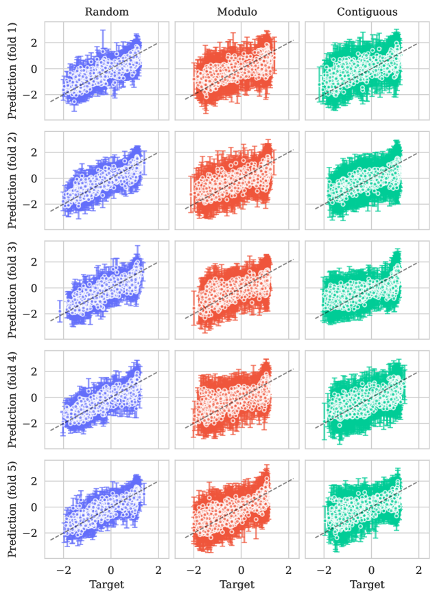
J.2 PA_I34A1_Wu_2015
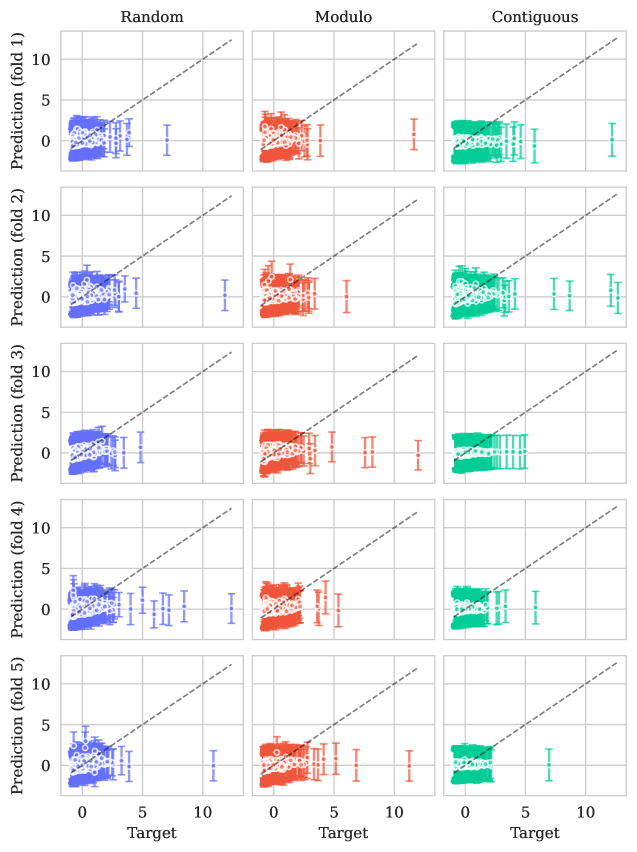
J.3 TCRG1_MOUSE_Tsuboyama_2023
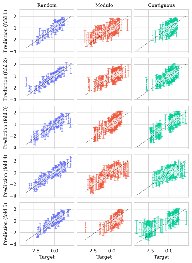
J.4 OPSD_HUMAN_Wan_2019
Appendix K Calibration curves for ProteinNPT
K.1 ProteinNPT details
We use ProteinNPT using the provided software in the paper with the default settings. We generate the MSA Transformer embeddings manually using the provided software from ProteinNPT. During evaluation, we predict using Monte Carlo dropout (with 25 samples, as described in the ProteinNPT appendix). An uncertainty estimate per test sequence is obtained by taking the standard deviation over the 25 samples as prescribed.
K.2 Calibration curves
K.3 Predicted vs. true values for calibration datasets
K.3.1 BLAT_ECOLX_Stiffler_2015
K.3.2 PA_I34A1_Wu_2015
K.3.3 TCRG1_MOUSE_Tsuboyama_2023
K.3.4 OPSD_HUMAN_Wan_2019
Appendix L Alternative zero-shot methods
Kermut uses a linear transformation of a variant’s zero-shot score as its mean function. In the main results ESM-2 was used. We here provide additional results where different zero-shot methods are used. The experiments are carried out as the ablation results in Section 4.1, i.e., on 174/217 datasets. All zero-shot scores are pre-computed and are available via the ProteinGym suite.
Using a zero-shot mean function instead of a constant mean evidently leads to increased performance. The magnitude of the improvement depends on the chosen zero-shot method, where the order roughly corresponds to that of the zero-shot scores in ProteinGym. We do however see that opting for EVE yields the largest performance increase.
| Zero-shot predictor | Spearman () | MSE () | ||||||
|---|---|---|---|---|---|---|---|---|
| Contig. | Mod. | Rand. | Avg. | Contig. | Mod. | Rand. | Avg. | |
| EVE | 0.610 | 0.628 | 0.750 | 0.663 | 0.729 | 0.680 | 0.412 | 0.607 |
| ESM-2∗ | 0.607 | 0.628 | 0.747 | 0.660 | 0.729 | 0.682 | 0.414 | 0.609 |
| VESPA | 0.605 | 0.622 | 0.742 | 0.657 | 0.736 | 0.697 | 0.424 | 0.619 |
| GEMME | 0.604 | 0.622 | 0.744 | 0.657 | 0.729 | 0.682 | 0.416 | 0.609 |
| TranceptEVE L | 0.597 | 0.617 | 0.744 | 0.653 | 0.742 | 0.694 | 0.420 | 0.618 |
| ESM-IF1 | 0.581 | 0.605 | 0.738 | 0.641 | 0.757 | 0.708 | 0.424 | 0.630 |
| ProteinMPNN | 0.573 | 0.599 | 0.734 | 0.635 | 0.769 | 0.717 | 0.429 | 0.638 |
| Constant mean | 0.568 | 0.595 | 0.735 | 0.633 | 0.771 | 0.718 | 0.429 | 0.639 |
Appendix M Ethics
We have introduced a general framework to predict variant effects given labelled data. The intent of our work is to use the framework to model and subsequently optimize proteins. We acknowledge that – in principle – any protein property can be modelled (depending on the available data), which means that potentially harmful proteins can be engineered using our method. We encourage the community to use our proposed method for beneficial purposes only, such as the engineering of efficient enzymes or for the characterization of potentially pathogenic variants for the betterment of biological interpretation and clinical treatment.
Appendix N License
The codebase will be made publicly available under the open source MIT License once anonymity is not an issue.
Appendix O Detailed results per DMS
We show the performance of Kermut and ProteinNPT per DMS assay in Figures 16, 17, 18 and 19. The figures show the average performance and the performance per split, respectively.
O.1 Detailed results per DMS (average)
O.2 Detailed results per DMS (random)
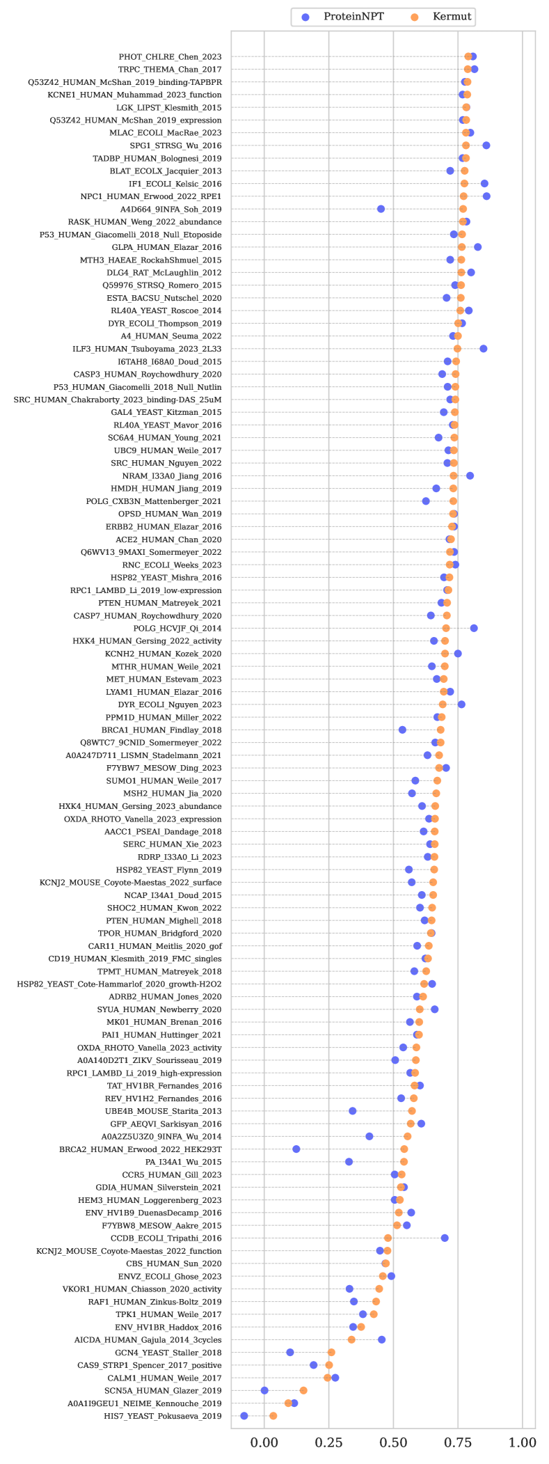
O.3 Detailed results per DMS (modulo)
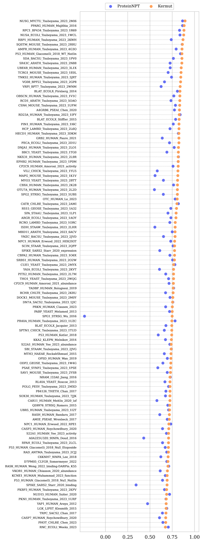
O.4 Detailed results per DMS (contiguous)
