Charge transport in organic semiconductors from the mapping approach to surface hopping

Abstract

We describe how to simulate charge diffusion in organic semiconductors using a recently introduced mixed quantum-classical method, the mapping approach to surface hopping. In contrast to standard fewest-switches surface hopping, this method propagates the classical degrees of freedom deterministically on the most populated adiabatic electronic state. This correctly preserves the equilibrium distribution of a quantum charge coupled to classical phonons, allowing one to time-average along trajectories to improve the statistical convergence of the calculation. We illustrate the method with an application to a standard model for the charge transport in the direction of maximum mobility in crystalline rubrene. Because of its consistency with the quantum-classical equilibrium distribution, the present method gives a time-dependent diffusion coefficient that plateaus correctly to a long-time limiting value. We end by comparing our results for the mobility and optical conductivity to those of the widely used relaxation time approximation, which uses a phenomenological relaxation parameter to obtain a non-zero diffusion coefficient from a calculation with static phonon disorder. We find that this approximation generally underestimates the charge mobility when compared with our method, which is parameter free and directly simulates the thermal equilibrium diffusion of a quantum charge coupled to classical phonons.

I Introduction

Soft organic semiconductors have attracted considerable attention as an emerging class of materials for organic light-emitting diodes, field-effect transistors, and photovoltaic devices.Fratini et al. (2020); Ghosh and Spano (2020) Their conductive properties can be understood in terms of charges diffusing through the material due to interaction with phonons. For the high-mobility materials of interest, the charge-phonon coupling is too weak to be explained entirely by a local hopping (polaronic) mechanism, yet too large for an entirely delocalised (band-like) mechanism.Oberhofer, Reuter, and Blumberger (2017) In recent years, a picture has emerged of an intermediate scenario in which dynamic disorder gives rise to transient localization.Fratini, Mayou, and Ciuchi (2016); Nematiaram and Troisi (2020); Giannini et al. (2023) This perspective has led to estimates of the charge mobility of a wide range of semiconductors within the relaxation time approximation.Fratini et al. (2017); Nematiaram et al. (2019); Harrelson et al. (2019); Landi (2019) However, it remains unclear how well this phenomenological picture compares to direct simulation due to the lack of reliable methods to simulate the coupled dynamics of charges and phonons.

While exact quantum methods have recently been used to address this problem,De Filippis et al. (2015); Li, Ren, and Shuai (2021); Li, Yan, and Shi (2024) they have so far been restricted to smaller systems and/or shorter time scales than we shall consider here. A more tractable strategy is to use mixed quantum-classical trajectories. In a pioneering study, Troisi and Orlandi showed that even the simple Ehrenfest approximation can capture the dynamical localization of a charge coupled to intermolecular phonons.Troisi and Orlandi (2006) However, the Ehrenfest approach is known to bring the system out of thermal equilibrium by leaking nuclear energy to the electronic subsystem.Parandekar and Tully (2005) As a result, the calculated diffusivity has been found not to reach a clear long-time plateau.Ciuchi, Fratini, and Mayou (2011); Fratini, Mayou, and Ciuchi (2016) Another popular quantum-classical method is Tully’s fewest switches surface hopping (FSSH),Tully (1990) variations of which are widely used to simulate organic semiconductors.Wang and Beljonne (2013); Wang, Prezhdo, and Beljonne (2015); Giannini et al. (2019); Carof, Giannini, and Blumberger (2019); Xie et al. (2020); Sneyd et al. (2021); Roosta et al. (2022); Peng et al. (2022) However, the treatment of electronic coherences in FSSH remains contentious Wang et al. (2020), and it is challenging to resolve the low hopping probabilities associated with a large number of weakly coupled electronic states.Wang and Beljonne (2013)

Despite their drawbacks, Ehrenfest dynamics and FSSH (with appropriate corrections) have been found to yield reasonable agreement with experiment for a variety of systems.Nematiaram and Troisi (2020) However, a remaining practical limitation is that the results of both methods need to be averaged over a large number of trajectories to obtain well-converged mobilities. We find it remarkable that so little progress has been made to reduce this effort when calculating linear response properties such as the thermal mobility. For adiabatic dynamics on a single electronic potential energy surface, it has long been standard practice to accelerate the calculation of time-correlation functions by averaging along equilibrium trajectories.Tuckerman (2010) Unfortunately, it is not possible to do this in the non-adiabatic case with Ehrenfest dynamics or FSSH, since neither of these methods preserves the equilibrium distribution of the coupled charge-phonon system.

In this paper, we shall show that one can in fact simulate charge diffusion with trajectories that preserve the quantum-classical equilibrium distribution, as is required for time averaging. Our starting point is the recently-developed ‘mapping approach to surface hopping’ (MASH). Mannouch and Richardson (2023); Runeson and Manolopoulos (2023) In contrast to the stochastic surface hopping of FSSH, this approach evolves trajectories deterministically on the adiabatic state with the largest population. MASH is consistent with the quantum–classical Boltzmann distribution,Runeson and Manolopoulos (2023); Amati, Mannouch, and Richardson (2023) and it has previously been shown to be successful for simulating excitonic systems with as many as eight coupled electronic states.Runeson, Fay, and Manolopoulos (2024); Lawrence, Mannouch, and Richardson (2024a) However, organic semiconductors pose an additional challenge in that they involve a band of many more (in practice, hundreds of) electronic states. Despite the apparent difficulty, we shall show that evolving on the most populated adiabatic state also works well in this context and is sufficient to overcome the overheating problem of Ehrenfest dynamics. In order to calculate the charge diffusion, we introduce a MASH estimator for the charge velocity operator and describe how to calculate its equilibrium time-correlation function. Since the resulting expression is time-translationally invariant, one can average it over time origins to accelerate the convergence with respect to the number of trajectories, which significantly reduces the cost of the calculation.

In Section II, we outline the problem of diffusion in organic semiconductors and describe our MASH methodology for solving it. In Section III, we apply this methodology to a Su-Schrieffer-Heeger (SSH) model for the charge mobility in crystalline rubrene, a molecular semiconductor for which there is a large body of previous experimental and theoretical work. We discuss our results for the time-dependent charge diffusion coefficient $D(t)$, the temperature-dependent charge mobility $\mu(T)$, and the frequency-dependent optical conductivity $\sigma(\omega)$ in light of this previous work. In particular, we highlight the differences between the present MASH results and those of Ehrenfest dynamics, the classical path approximation (CPA),Wang et al. (2011); Fetherolf, Golež, and Berkelbach (2020); Fetherolf, Shih, and Berkelbach (2023) and the relaxation time approximation (RTA),Ciuchi, Fratini, and Mayou (2011); Cataudella, De Filippis, and Perroni (2011); Fratini, Mayou, and Ciuchi (2016) all three of which are still widely used to study charge transport in organic semiconductors. Our conclusions are drawn in Section IV.

II Theory

II.1 Hamiltonian and Observables

A standard model of a charge (an electron or a hole) interacting with phonons in an organic semiconductor is provided by the SSH Hamiltonian

$$\hat{H}(p,q)= \sum_{j}\Bigl{(}-J+\alpha[\hat{q}_{j}-\hat{q}_{j+1}]\Bigr{)}\Bigl{(}|j\rangle\langle j+1|+|j+1\rangle\langle j|\Bigr{)}$$

$$+\sum_{j}\Bigl{(}\frac{\hat{p}_{j}^{2}}{2m}+\frac{1}{2}m\omega_{0}^{2}\hat{q}_{j}^{2}\Bigr{)},$$ (1)

where the index $j$ runs over the molecules along a particular lattice direction in the molecular crystal. The ket $|j\rangle$ is a basis state in which the charge is located on molecule $j$. The Hamiltonian involves a nearest neighbour interaction that fluctuates around an average value of $J$ as a result of Peierls coupling to harmonic phonons. The position of the charge in the model is represented by the operator

$$\hat{x}=\sum_{j}aj\,|j\rangle\langle j|,$$ (2)

where $a$ is the equilibrium intermolecular spacing between the molecules. This model assumes that the material is sufficiently anisotropic to consider only one-dimensional diffusion, and that the effect of any Holstein coupling to high frequency intramolecular phonons has already been folded into the definition of the parameters $J$ and $\alpha$ with a polaron transformation.Nematiaram and Troisi (2020)

The key experimental observable is the mobility $\mu$ of the charge, which is related to its diffusion coefficient by the Einstein–Smoluchowski equation $\mu={eD/k_{\rm B}T}$. The diffusion coefficient $D$ can be written as the long-time limit of a time-dependent diffusion coefficient

$$D(t)=\frac{1}{2}\frac{\rm d}{\mathrm{d}t}\Delta x^{2}(t)\equiv\int_{0}^{t}C(t^{\prime})\,{\rm d}t^{\prime},$$ (3)

where $\Delta x^{2}(t)$ is the mean squared displacement of the charge in time $t$,

$$\Delta x^{2}(t)=\left<\left[\hat{x}(t)-\hat{x}(0)\right]^{2}\right>,$$ (4)

and $C(t)$ is its velocity autocorrelation function

$$C(t)=\frac{1}{2}\Bigl{<}\hat{v}(0)\hat{v}(t)+\hat{v}(t)\hat{v}(0)\Bigr{>}.$$ (5)

Here $\hat{x}(t)$ and $\hat{v}(t)$ are the Heisenberg operators $\hat{A}(t)=e^{+i\hat{H}t/\hbar}\hat{A}\,e^{-i\hat{H}t/\hbar}$, the velocity operator $\hat{v}=(i/\hbar)[\hat{H},\hat{x}]$ is the Heisenberg time derivative of $\hat{x}$, and the expectation values are with respect to the thermal equilibrium distribution

$$\left<\cdots\right>={{\displaystyle{\rm tr}\left[e^{-\beta\hat{H}}(\cdots)\right]}\over{\displaystyle{\rm tr}\left[e^{-\beta\hat{H}}\right]}},$$ (6)

where $\beta=1/k_{\rm B}T$.

More detailed information about the diffusive process can be obtained by measuring the frequency-dependent optical conductivity $\sigma(\omega)$. This is related to $C(t)$ byCiuchi, Fratini, and Mayou (2011)

$$\sigma(\omega)=ne^{2}\,{\tanh(\beta\hbar\omega/2)\over\hbar\omega/2}\,{\rm Re}\int_{0}^{\infty}e^{+i\omega t}C(t)\,{\rm d}t,$$ (7)

where $n$ is the number density of charges in the crystal. The low-frequency limit of $\sigma(\omega)$ is directly related to $\mu$ through $\sigma(\omega\to 0)=ne\mu$, and its behaviour at higher frequencies is readily available from a calculation of the velocity autocorrelation function $C(t)$.

In what follows we will assume that the temperature is sufficiently high ($k_{\rm B}T>\hbar\omega_{0}$) that the vibrations can be treated classically ($\hat{p}_{j}\to p_{j}$ and $\hat{q}_{j}\to q_{j}$), as is certainly the case for the rubrene model considered in Sec. III. To avoid boundary effects in a finite chain of $N$ molecules, we also will apply periodic boundary conditions by setting $|N+1\rangle\equiv|1\rangle$, $p_{N+1,k}\equiv p_{1}$, and $q_{N+1}\equiv q_{1}$ in both the Hamiltonian and the velocity operator

$$\hat{v}(q)=\frac{i}{\hbar}\sum_{j=1}^{N}aJ_{j}(q)\Bigl{(}|j+1\rangle\langle j|-|j\rangle\langle j+1|\Bigr{)}$$ (8)

where

$$J_{j}(q)=-J+\alpha[q_{j}-q_{j+1}].$$ (9)

Note in passing that the matrix representation of this velocity operator is purely imaginary in the site basis, with zero elements on the diagonal. These properties also hold in any other real basis, including the adiabatic basis introduced below.

II.2 Quantum-Classical Dynamics

When periodic boundary conditions are applied to an $N$-molecule chain with classical vibrational modes as we have described above, the Hamiltonian in Eq. (1) can be written more compactly as

$$\hat{H}=T(p)+\hat{V}(q),$$ (10)

where $q=\left\{q_{j}\right\}$ and $p=\left\{p_{j}\right\}$ are the coordinates and momenta of the classical vibrations, $T(p)$ is the vibrational kinetic energy

$$T(p)=\sum_{j=1}^{N}{p_{j}^{2}\over 2m},$$ (11)

and $\hat{V}(q)$ is a potential energy operator

$$\hat{V}(q)=\sum_{i=1}^{N}\sum_{j=1}^{N}|i\rangle V_{ij}(q)\langle j|.$$ (12)

The diagonal representation of this operator is

$$\hat{V}(q)=\sum_{a=1}^{N}|a(q)\rangle V_{a}(q)\langle a(q)|,$$ (13)

where $V_{a}(q)$ are the adiabatic potential energy surfaces and $|a(q)\rangle$ are the adiabatic eigenstates at the configuration $q$. A normalized wavefunction $|c\rangle$ for the charge can be written equivalently in either representation as

$$|c\rangle=\sum_{j=1}^{N}|j\rangle\,c_{j}=\sum_{a=1}^{N}|a(q)\rangle\,c_{a}.$$ (14)

In all of the trajectory methods described below, this wavefunction satisfies the Schrödinger equation of motion

$$|\dot{c}\rangle=-\frac{i}{\hbar}\hat{V}(q)|c\rangle,$$ (15)

and the classical degrees of freedom satisfy equations of motion of the form

$$\dot{q}_{j} =p_{j}/m$$ (16)

$$\dot{p}_{j} =F_{j}(q),$$ (17)

but with different definitions of the force $F_{j}(q)$:

• In the CPA, one completely neglects the feedback of the quantum state on the classical degrees of freedom. For the SSH Hamiltonian, this prescription corresponds to

  $$F_{j}(q)=-m\omega_{0}^{2}q_{j}.$$ (18)

  This approximation is equivalent to the approach considered in Refs. Wang et al., 2011; Fetherolf, Golež, and Berkelbach, 2020; Fetherolf, Shih, and Berkelbach, 2023.

• In (mean-field) Ehrenfest dynamics, the effective force is the expectation value of the force operator,

  $$F_{j}(q)=-\langle c|\nabla_{j}\hat{V}(q)|c\rangle,$$ (19)

  which can be evaluated using either of the representations in Eq. (14). This method is commonly used for charge transport in organic semiconductors.Troisi and Orlandi (2006); Troisi (2007); Wang et al. (2011); Poole et al. (2016); Hegger, Binder, and Burghardt (2020); Berencei, Barford, and Clark (2022)

• In MASH, we use the force of the highest populated adiabatic state. By introducing the “step function”

  $$\Theta_{a}(c)=\begin{cases}1,&\hbox{if }|c_{a}|^{2}>|c_{b}|^{2}\hbox{ for all }b\not=a,\\ 0,&\hbox{otherwise},\end{cases}$$ (20)

  this force can be written as

  $$F_{j}(q)=-\sum_{a}\nabla_{j}V_{a}(q)\Theta_{a}(c).$$ (21)

Since we are interested in the dynamical properties of a mixed quantum-classical system at thermal equilibrium, the relevant expectation values are with respect to quantum-classical limit of Eq. (6),

$$\langle\cdots\rangle=\frac{\int\mathrm{d}p\,\mathrm{d}q\,\mathrm{tr}_{\mathrm{el}}[e^{-\beta\hat{H}(p,q)}(\cdots)]}{\int\mathrm{d}p\,\mathrm{d}q\,\mathrm{tr}_{\mathrm{el}}[e^{-\beta\hat{H}(p,q)}]}.$$ (22)

However, neither the CPA nor Ehrenfest dynamics is consistent with this distribution.Parandekar and Tully (2006) With these methods, even a system initially in equilibrium will experience an unphysical flow of energy from the classical to the quantum subsystem, leading to long-time populations that correspond to an elevated temperature (in the case of the CPA, this temperature is infiniteRuneson et al. (2022)). MASH, on the other hand, is consistent with the correct distribution by virtue of the identityRuneson and Manolopoulos (2023)

$$\langle\cdots\rangle=\int\mathrm{d}p\,\mathrm{d}q\int_{|c|=1}\mathrm{d}c\,\rho(p,q,c)\sum_{a}\langle a(q)|\cdots|a(q)\rangle\Theta_{a}(c),$$ (23)

where

$$\rho(p,q,c)=\frac{e^{-\beta E(p,q,c)}}{\int\mathrm{d}p\,\mathrm{d}q\int_{|c|=1}\mathrm{d}c\,e^{-\beta E(p,q,c)}}$$ (24)

is the Boltzmann density corresponding to the energy

$$E(p,q,c)=T(p)+\sum_{a}V_{a}(q)\Theta_{a}(c).$$ (25)

In these equations, $c$ plays the role of a complex vector of phase-space variables for the quantum degree of freedom rather than a wavefunction.

To handle hops in MASH, it is helpful to think of the term $\sum_{a}V_{a}(q)\Theta_{a}(c)$ in Eq. (25) as an effective step potential in the phase space $(p,q,c)$. When the active adiabatic state changes from $a$ to $b$, the adiabatic potential changes from $V_{a}(q)$ to $V_{b}(q)$. If the component $p_{\perp}$ of the momentum perpendicular to the step has sufficient kinetic energy to overcome it, the transition is successful and $p_{\perp}$ is scaled in such a way as to conserve $E(p,q,c)$. If not, the transition is unsuccessful and the trajectory is reflected from the step with a reversal of $p_{\perp}$, which has the effect of restoring $a$ as the active state and enabling the nuclear motion to continue on $V_{a}(q)$. By analysing the terms in Eq. (21), one can show that $p_{\perp}$ is the projection of $p$ along the direction of the vector with elementsRuneson and Manolopoulos (2023)

$$\delta_{j}=\operatorname{Re}\sum_{a^{\prime}}c_{a^{\prime}}(d^{j}_{a^{\prime}a}c_{a}-d^{j}_{a^{\prime}b}c_{b})$$ (26)

where $d_{ab}^{j}=\langle a(q)|\nabla_{j}|b(q)\rangle$ is an element of the non-adiabatic coupling vector between adiabatic states $a$ and $b$.

This deterministic surface hopping algorithm clearly conserves both $E(p,q,c)$ and $\rho(p,q,c)$, and since it is equivalent to integrating Eqs. (15)–(17) across a smoothed step it also conserves the phase space volume element ${\rm d}p\,{\rm d}q\,{\rm d}c$. Hence, the MASH dynamics relaxes to the correct quantum-classical equilibrium state populations.Amati, Mannouch, and Richardson (2023) This is in contrast to the stochastic FSSH algorithm, which does not in general relax to the correct equilibrium populations.Schmidt, Parandekar, and Tully (2008)

II.3 Velocity autocorrelation function

Next, we describe how to calculate the velocity autocorrelation function in Eq. (5) in the different methods. In the CPA and Ehrenfest dynamics, we first rewrite $C(t)$ as

$$C(t)=\frac{\int\mathrm{d}p\,\mathrm{d}q\sum_{a}e^{-\beta[T(p)+V_{a}(q)]}C_{a}(t)}{\int\mathrm{d}p\,\mathrm{d}q\sum_{a}e^{-\beta[T(p)+V_{a}(q)]}}$$ (27)

where

$$C_{a}(t)=\operatorname{Re}\,\langle a|\hat{v}e^{+i\hat{H}t/\hbar}\hat{v}e^{-i\hat{H}t/\hbar}|a\rangle.$$ (28)

We initialize trajectories by sampling $p$ and $q$ from the Boltzmann distribution for uncoupled phonons. Then, for each $q$, we sample an adiabatic state $a$ from the Boltzmann distribution $e^{-\beta V_{a}(q)}/\sum_{a}e^{-\beta V_{a}(q)}$ and initialize the wavefunction as $|a\rangle$. Along the trajectory, we propagate $|a(t)\rangle$ from $|a\rangle$ and $|va(t)\rangle$ from $|va\rangle\equiv\hat{v}|a\rangle$ with the Schrödinger equation. Then we evaluate

$$C_{a}(t)=\operatorname{Re}\,\langle va(t)|\hat{v}|a(t)\rangle$$ (29)

and average over trajectories. Note that this two-step sampling procedure generates an initial distribution that is not strictly the same as the true coupled Boltzmann distribution. We use it here for consistency with previous workCiuchi, Fratini, and Mayou (2011); Fratini, Mayou, and Ciuchi (2016), noting that the initial conditions should not affect long-time properties such as the mobility.

In MASH, it is possible to construct another approximation to $C(t)$ that looks closer to an ordinary classical correlation function. The derivation is given in the Appendix so here we shall simply state the result: $C(t)$ can be calculated as the canonical phase space average

$$C(t)=\langle v(q_{0},c_{0})v(q_{t},c_{t})\rangle,$$ (30)

where

$$\langle\cdots\rangle=\int{\rm d}p_{0}{\rm d}q_{0}\int_{|c_{0}|=1}{\rm d}c_{0}\,\rho(p_{0},q_{0},c_{0})(\cdots)$$ (31)

and

$$v(q,c)=\sqrt{1\over 2\Gamma}\sum_{a=1}^{N}\sum_{b=1}^{N}v_{ab}(q)\Theta_{ab}(c)c_{a}^{*}c_{b}$$ (32)

with $v_{ab}(q)=\langle a(q)|\hat{v}(q)|b(q)\rangle$ and $\Theta_{ab}(c)=\Theta_{a}(c)+\Theta_{b}(c)$. The constant $\Gamma$ is

$$\Gamma={H_{N}\over N(N-1)}-{H_{N}^{2}+G_{N}\over(N+1)N(N-1)},$$ (33)

where $H_{N}=\sum_{n=1}^{N}1/n$ and $G_{N}=\sum_{n=1}^{N}1/n^{2}$.

Since the MASH dynamics conserves both the Boltzmann factor $\rho(p_{0},q_{0},c_{0})$ and the phase-space volume element ${\rm d}p_{0}\,{\rm d}q_{0}\,{\rm d}c_{0}$, we can also write

$$C(t)=\langle v(q_{\tau},c_{\tau})v(q_{\tau+t},c_{\tau+t})\rangle$$ (34)

for any time origin $\tau$. This is especially useful because it allows us to time-average along our trajectories and write the correlation function as

$$C(t)={1\over T}\int_{0}^{T}{\rm d}\tau\,\langle v(q_{\tau},c_{\tau})v(q_{\tau+t},c_{\tau+t})\rangle,$$ (35)

which significantly reduces the statistical error in the calculation. To generate an equilibrium ensemble in practice, we first pre-equilibrate by running MASH from an adiabatically sampled initial condition in the presence of a thermostat. In the calculations presented below, we found that the equilibration phase only needed to be a small fraction (10%) of the total time used to calculate the correlation function.

III Results and Discussion

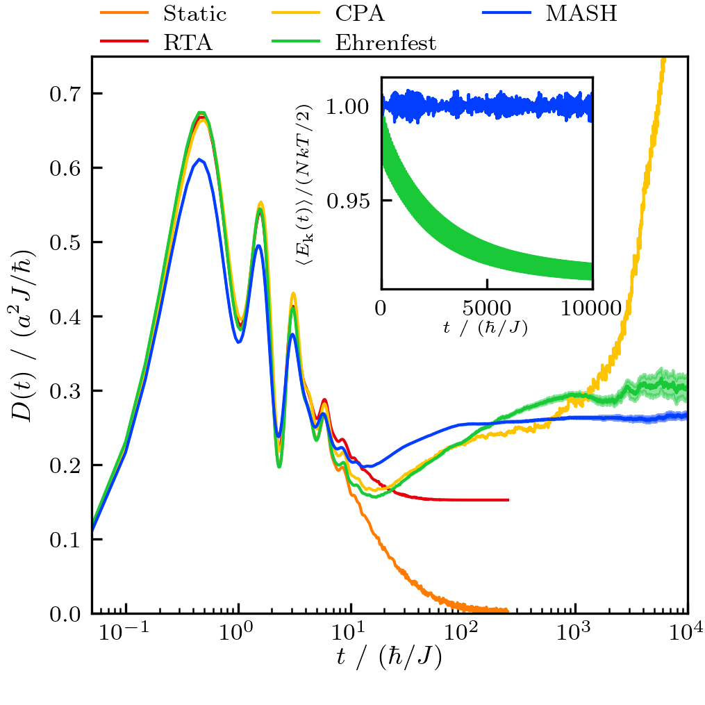
Figure 1: Time-dependent diffusivities at $T=$300\text{\,}\mathrm{K}$$ ($k_{\rm B}T=0.235J$). The diffusion coefficient $D(\infty)$ is zero in the Static calculation and undefined in the CPA and Ehrenfest dynamics. The MASH calculation gives a well-defined diffusion coefficient and the RTA gives a different one that depends on the choice of the relaxation time (the result shown here is for $\tau=23\,\hbar/J$). Inset: the initial phonon kinetic energy leaks into the electronic subsystem in Ehrenfest dynamics but fluctuates around the correct thermal equilibrium value in MASH.

We have performed our simulations for the SSH model in Eq. (1) with the parameters $J=$110\text{\,}\mathrm{m}\mathrm{e}\mathrm{V}$$ ($887\text{\,}\mathrm{c}\mathrm{m}^{-1}$), $\hbar\omega_{0}=0.0435J$ ($40\text{\,}\mathrm{c}\mathrm{m}^{-1}$), and $\lambda=\alpha^{2}/(2m\omega_{0}^{2}J)=0.25$. There are several sets of slightly different parameters in the literature and these particular parameters were chosen to be consistent with Ref. Ciuchi, Fratini, and Mayou, 2011. There is no need to specify the mass $m$ because it does not affect the diffusion of the charge. In practice we work with mass-scaled coordinates so $m$ does not even enter our calculation. We used $N=100$ sites with periodic boundary conditions and a lattice spacing of $a=$7.2\text{\,}\AA$$. The time step was set to $0.05\hbar/J$ ($0.3\text{\,}\mathrm{f}\mathrm{s}$) in all simulations.

III.1 Time-dependent diffusivity

To illustrate the importance of dynamical disorder, we first consider the static limit in which the phonon degrees of freedom are disordered at time $t=0$ and then kept frozen. For this scenario, the velocity autocorrelation function $C_{0}(t)$ can be easily computed in the eigenbasis of the disordered Hamiltonian, and then averaged over realisations of the disorder. As was shown by Ciuchi et al.,Ciuchi, Fratini, and Mayou (2011) and is shown again here in Fig. 1, the static limit leads to a time-dependent diffusivity that initially rises ballistically (super-diffusion), then falls (sub-diffusion) and eventually decays to zero as a result of Anderson localization. In other words, the mobility vanishes in this one-dimensional model when the phonons are frozen because the charge is stuck in a localised eigenstate.

A crude estimate of the mobility can nevertheless be extracted from the static phonon calculation by invoking a relaxation time approximation.Ciuchi, Fratini, and Mayou (2011); Cataudella, De Filippis, and Perroni (2011); Fratini, Mayou, and Ciuchi (2016) This assumes that the coherent evolution in the static picture decays over some phenomenological timescale $\tau$ such that

$$C_{\mathrm{RTA}}(t)=C_{0}(t)e^{-t/\tau}.$$ (36)

This results in a finite mobility that is proportional to the long-time diffusivity calculated from the time integral of $C_{\mathrm{RTA}}(t)$. Usually one chooses the relaxation time to be $\tau=\omega_{0}^{-1}$, i.e., to correspond to the timescale of the phonon motion ($\tau=23\,\hbar/J$ for the present model). The result of a RTA calculation with this value of $\tau$ is also shown in Fig. 1.

Next, we consider what the various quantum-classical simulation methods predict about the effect of dynamical disorder. In Ehrenfest dynamics, the diffusivity follows the static curve up to $t\approx 10\,\hbar/J$, after which it increases and eventually plateaus. (Ciuchi et al.Ciuchi, Fratini, and Mayou (2011) stopped their Ehrenfest calculation with the present parameters at $t\sim 10^{2}\,\hbar/J$, which gave them the impression that a plateau would not be reached.) However, because Ehrenfest dynamics suffers from an unphysical energy transfer from the phonons to the electronic degree of freedom, the plateau does not correspond to a genuine thermal equilibrium mobility. The energy transfer can be monitored by calculating the decay of the average kinetic energy of the phonons along the trajectories of the Ehrenfest simulation. This is shown in the inset of Fig. 1. The electronic system is clearly not in thermal equilibrium with the phonons in the plateau region, but rather in a non-equilibrium steady state.

In the case of the CPA, the phonons are uncoupled harmonic oscillators so their average kinetic energy does not decay – it simply fluctuates around the thermal equilibrium value of $Nk_{\rm B}T/2$. However, the electronic subsystem still heats up because it is being driven by a periodically oscillating field, and the effect of this on the long-time diffusivity is even worse than in Ehrenfest dynamics (compare the green and yellow curves in Fig. 1). On a linear scale it may appear as if the diffusivity has reached a plateau in both of these methods by the time $t\approx 20\,\hbar/J$, but it is clear from Fig. 1 that this is not the case. So when mobilities are reported using these methods one should be aware that they depend on the time at which the calculation was truncated.

In the MASH calculation, the diffusivity reaches a well-defined plateau on the same time scale as the RTA. The long-time limit of the diffusivity is unambiguous, and there is no need to choose a phenomenological relaxation time. This is because MASH is consistent with the quantum-classical equilibrium distribution, which precludes any unphysical overheating of the electronic subsystem. The MASH phonon kinetic energy in the inset of Fig. 1 fluctuates around the correct thermal equilibrium value of $Nk_{\rm B}T/2$. The short-time behaviour of the diffusivity obtained from MASH does differ slightly from that of the other approaches, but that is simply because the MASH calculation starts from the coupled equilibrium distribution (as explained in Sec. II.3).

The time-averaging along the equilibrium trajectories in MASH also helps to improve the convergence of the calculation. The shaded areas around the blue and green curves in Fig. 1 show the standard errors in the mean from 10 batches of $1000$ trajectories for MASH, and for 10 batches of $50\,000$ trajectories for Ehrenfest dynamics. (The CPA and Static curves are shown without error bars and were obtained from runs of 100 000 and 10 000 trajectories, respectively. The RTA curve was obtained by post-processing the results of the Static calculation.) The statistical error in the MASH calculation with time averaging is clearly far smaller than that in the Ehrenfest calculation without time averaging, especially in the diffusive regime.

Unfortunately, this does not make the MASH calculation any cheaper than the Ehrenfest calculation, because MASH requires an $O(N^{3})$ matrix diagonalisation at each time step to find the adiabatic states whereas Ehrenfest dynamics only requires $O(N)$ operations per time step (for the present model problem) when the wavefunction is evolved in the site basis. We are currently exploring ways to avoid a full matrix diagonalisation at each time step and make the MASH calculation cheaper, which will be useful for future applications of the method to more sophisticated (2D and 3D) models of charge transport in crystalline materials.

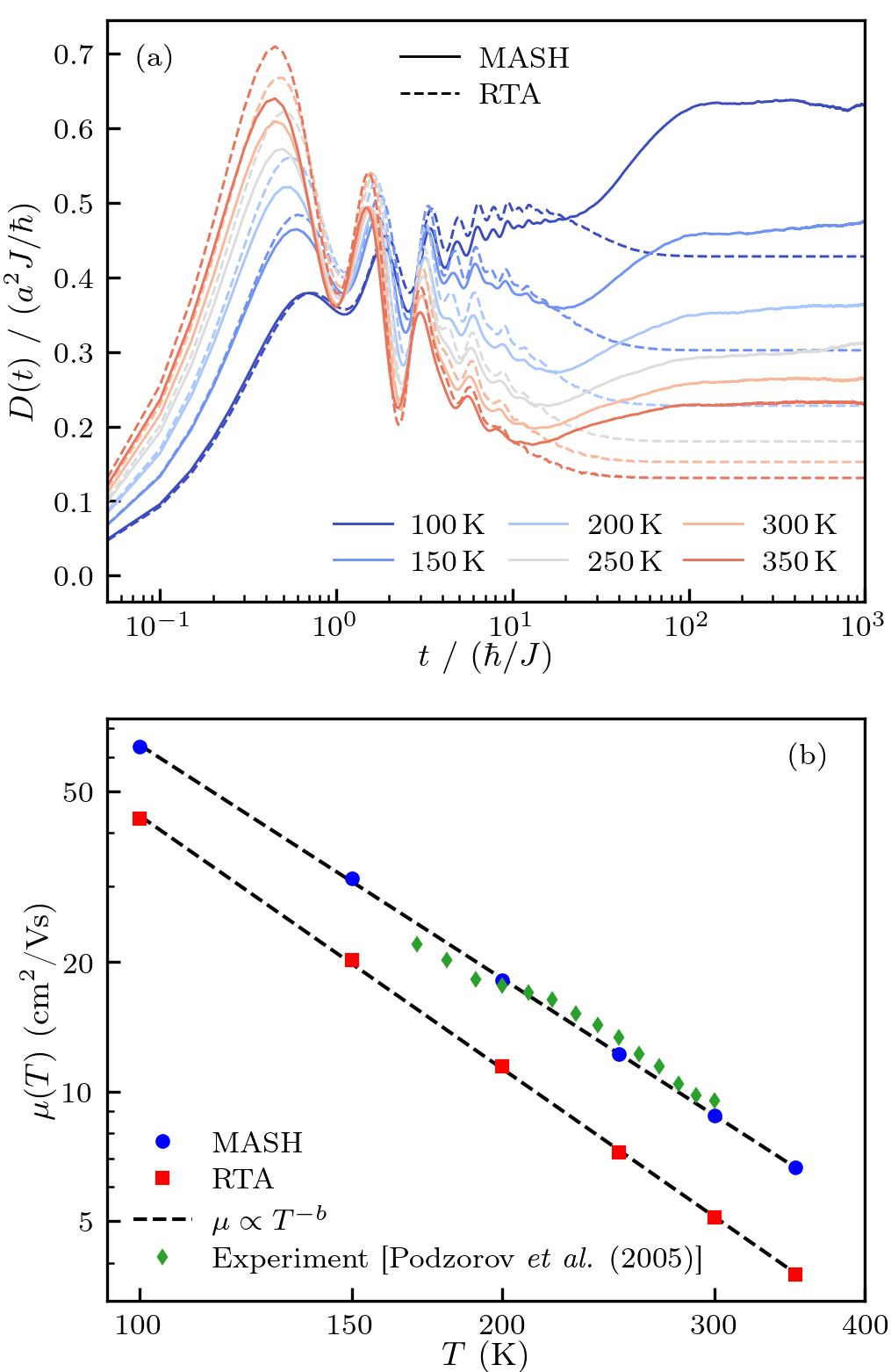
Figure 2: (a) MASH and RTA time-dependent diffusivities for a range of temperatures. (b) Log-log plot of the resulting mobilities as a function of temperature, and their fits to an inverse power law. Both calculations are seen to be qualitatively consistent with the results of a representative experiment from Ref. Podzorov et al., 2005.

III.2 Temperature-dependent mobility

We will now confine our attention to MASH and the RTA since these are the only two methods that give a well-defined mobility within a reasonable simulation time ($t\sim 10^{2}\,\hbar/J$). Figure 2(a) shows the time-dependent diffusivities obtained from these methods over a range of temperatures. Each MASH (RTA) curve was calculated from a single batch of 1000 (10 000) trajectories, and we again used a relaxation time of $\tau=\omega_{0}^{-1}$ in the RTA. A notable feature of the results is that the long-time plateau value of the diffusivity is consistently higher (by between 30 and 60%) in the MASH calculation than in the RTA. This discrepancy is comparable to the sensitivity of the RTA mobility to different choices of $\tau$.Cataudella, De Filippis, and Perroni (2011)

Figure 2(b) shows a log-log plot of the mobilities $\mu=eD(\infty)/k_{\rm B}T$ obtained from the MASH and RTA calculations as a function of temperature. Both methods give mobilities that follow an inverse power law $\mu\propto T^{-b}$, with $b=1.8$ for MASH and $b=2.0$ for the RTA (with $\tau=\omega_{0}^{-1}$). Both are in qualitative agreement with available experiments, as can be seen from the comparison with the mobilities of Podzorov et al.Podzorov et al. (2005) in the figure. Quantitative comparisons should be avoided, however, because the theoretical results are sensitive to the SSH model parameters and the experimental results are sensitive to both the quality of the crystal sample and the details of the experimental setup. The quantitative agreement between the MASH results and the experimental results in Fig. 2 is therefore fortuitous.

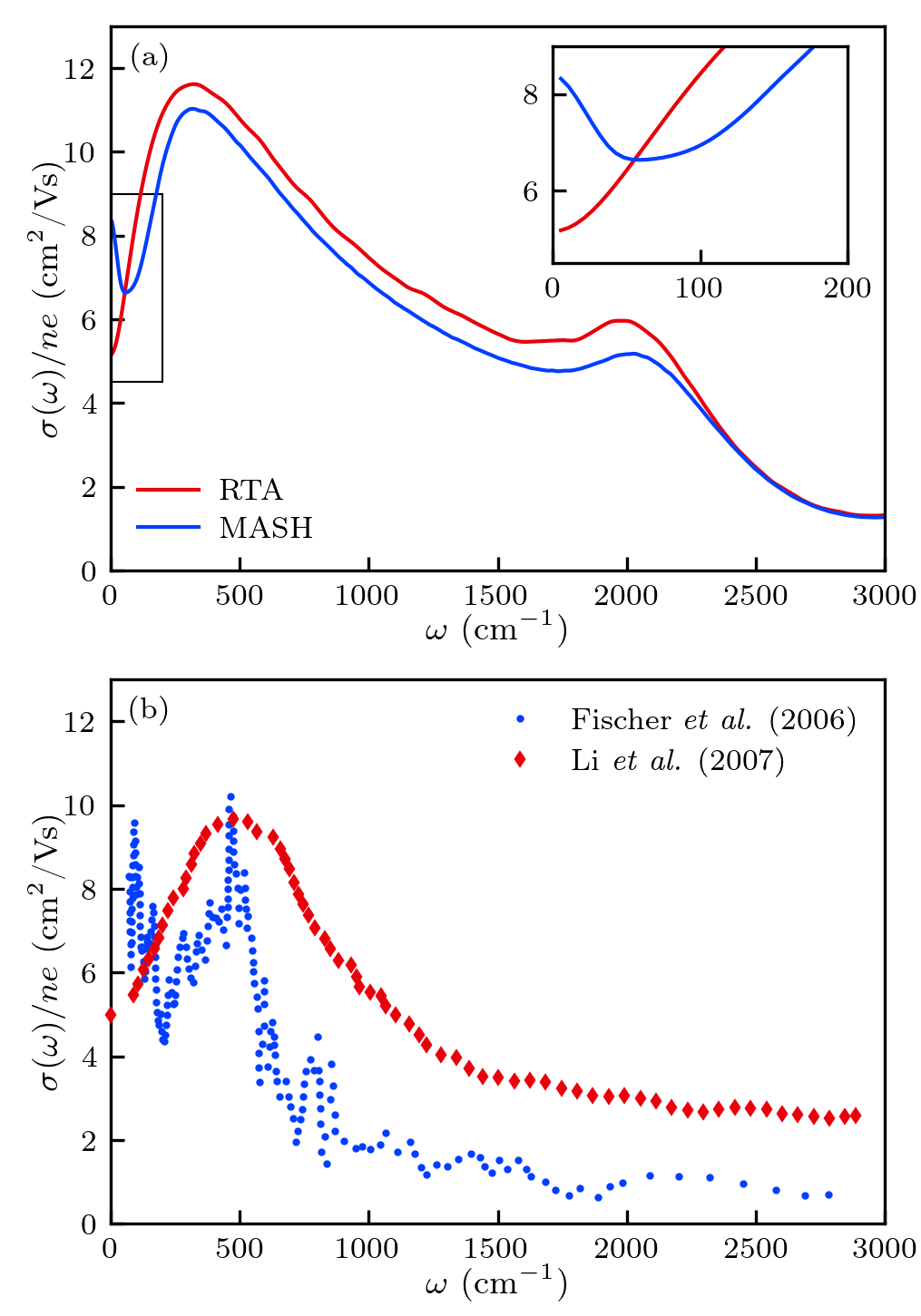
Figure 3: (a) MASH and RTA optical conductivities at $T=$300\text{\,}\mathrm{K}$$. As the frequency goes to zero (magnified in the inset), the RTA curve decreases smoothly to the zero-frequency mobility, whereas the MASH curve turns up as a result of the long-time rise of $D(t)$ observed in Fig. 1. (b) Available experimental resultsFischer et al. (2006); Li et al. (2007) are qualitatively consistent with either of these behaviours. The experimental data have been scaled such that the lowest-frequency point is the reported DC mobility, $8.3\text{\,}\mathrm{c}\mathrm{m}^{2}\mathrm{/}\mathrm{V}\mathrm{s}$ for Fischer et al. (Ref. Fischer et al., 2006) and $5\text{\,}\mathrm{c}\mathrm{m}^{2}\mathrm{/}\mathrm{V}\mathrm{s}$ for Li et al. (Ref. Li et al., 2007).

III.3 Frequency-dependent optical conductivity

Further insight into the differences between the MASH and RTA calculations can be obtained by comparing their predictions for the optical conductivity. This comparison is shown for a temperature of 300 K in the upper panel of Fig. 3. Both calculations predict a main peak in $\sigma(\omega)$ at around 400 cm^-1, and a smaller peak at around 2000 cm^-1. These peaks come from short-time oscillations in the velocity autocorrelation function that give rise to the structure below $t\sim 10\,\hbar/J$ in $D(t)$, which is similar in the two calculations (see Fig. 1). Where the calculations differ is in the behaviour of the optical conductivity as $\omega\to 0$. The RTA predicts a smooth decrease in $\sigma(\omega)$ below the peak at 400 cm^-1,Fratini, Ciuchi, and Mayou (2014) whereas MASH predicts a low frequency rise. This rise comes from a long-time tail in the MASH velocity autocorrelation function that is responsible for the increase of the MASH $D(t)$ to its plateau value in Fig. 1. The tail is absent by construction in the RTA because it is not present in the static disorder calculation that produces $C_{0}(t)$, and even if it were present it would be eliminated by the factor of $e^{-t/\tau}$ in Eq. (36).

The lower panel of Fig. 3 shows two representative optical conductivity spectra of crystalline rubrene at 300 K. These were measured using different crystal samples in different laboratories with different experimental setups.Fischer et al. (2006); Li et al. (2007) Neither experiment shows any evidence for a second peak in the optical conductivity at 2000 cm^-1, which is therefore likely to be a deficiency of the SSH model we have used in our calculations. The measurement by Li et al.Li et al. (2007) also does not show any evidence of a low-frequency rise in $\sigma(\omega)$, but the measurement by Fischer et al.Fischer et al. (2006) does. The experimental evidence for a low frequency rise in $\sigma(\omega)$ caused by a long-time tail in $C(t)$ is therefore inconclusive.

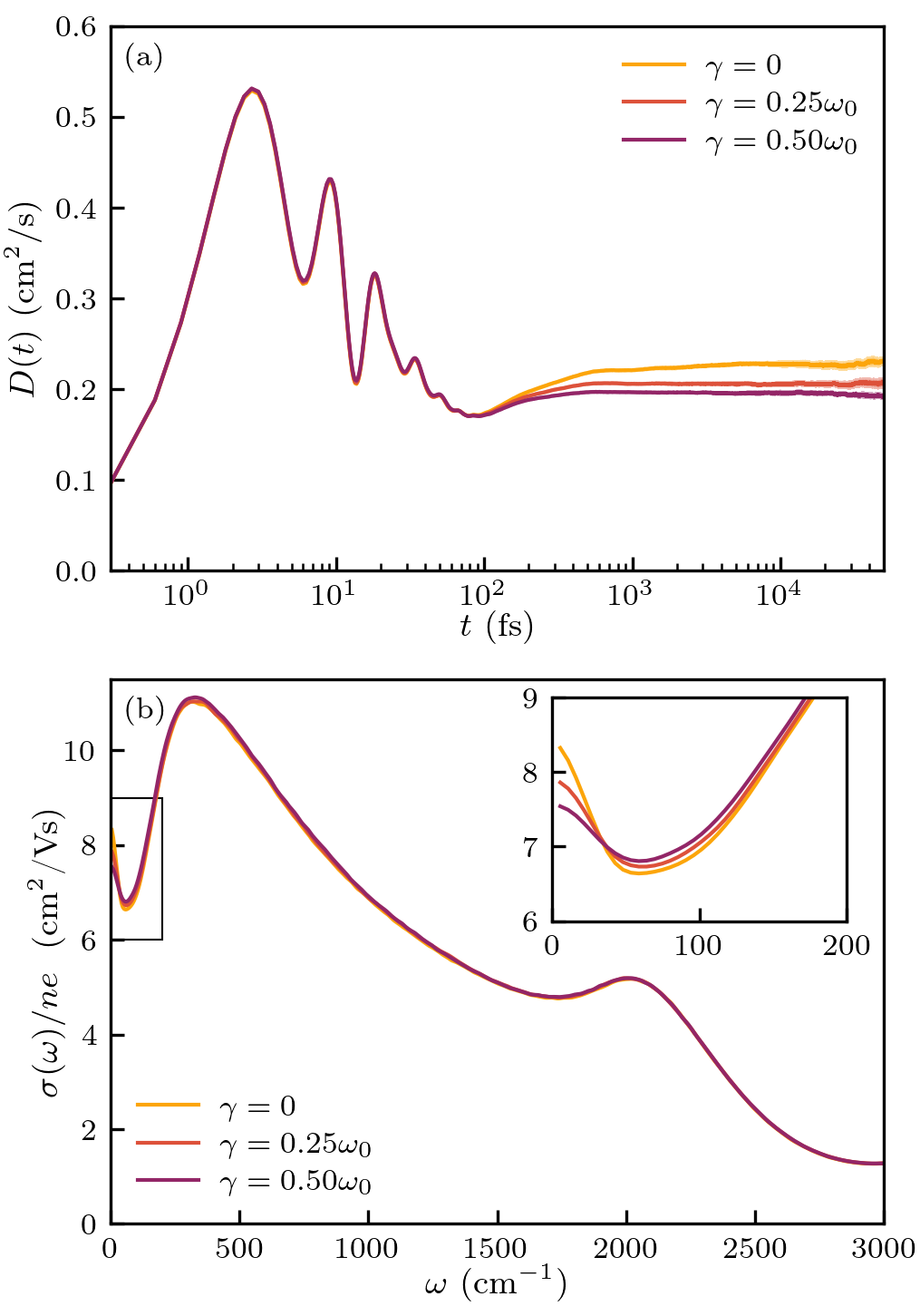
Figure 4: Impact of friction on the MASH dynamics. Increased friction leads to a reduction in (a) the long-time limit of the time-dependent diffusivity, and (b) the low-frequency limit of the optical conductivity.

The low-frequency rise in the MASH calculation is only seen below $\omega_{0}$ ($40\text{\,}\mathrm{c}\mathrm{m}^{-1}$), indicating that it is related to phonon motion. It is conceivable that the present model, which only includes a single-frequency phonon mode, is insufficient to represent the dynamics in a real material. A more realistic model would include a continuous density of phonon frequencies. For example, anharmonicity will effectively broaden the lineshape of the phonon spectrum,

$$L(\omega)=\int_{-\infty}^{\infty}\mathrm{d}t\,e^{-i\omega t}\langle q_{j}(0)q_{j}(t)\rangle.$$ (37)

A practical way to mimic this effect is to add Langevin friction to the dynamics, so that Eq. (17) becomes Nitzan (2006); Troisi and Cheung (2009)

$$\dot{p}_{j}=F_{j}(q)-\gamma p_{j}+R_{j}(t)$$ (38)

where $\gamma$ is a friction parameter and $R_{j}(t)$ is a random force that obeys $\langle R_{j}(t)R_{j}(0)\rangle=2m\gamma k_{\mathrm{B}}T\delta(t)$. In the underdamped regime ($\gamma<\omega_{0}$), $\gamma$ is approximately equal to full width at half maximum of the lineshape $L(\omega)$. Based on the phonon spectrum in Fig. 1 of Ref. Troisi, 2007, which is dominated by a single broad peak, we estimate a realistic friction to be on the order of $\gamma\approx\omega_{0}/4$. To explore the effect of friction on the MASH dynamics, Fig. 4 shows the results with $\gamma=0.25\,\omega_{0}$ and $\gamma=0.5\,\omega_{0}$. In comparison to the frictionless model, the only difference is in the dampening of the long-time dynamics and the associated low-frequency feature in the optical conductivity. Since other sources of dissipation may also damp out this feature, and since the amount of dissipation seen in an experiment is likely to depend on various factors including the quality of the crystalline sample, this may help to explain why the low-frequency feature is observed in one experiment in Fig. 3(b) and not in the other.

IV Conclusions

In this paper, we have presented a mixed quantum–classical method to simulate charge diffusion in molecular semiconductors at thermal equilibrium. The method solves the overheating problem of Ehrenfest dynamics and the CPA and it gives a well-defined long-time diffusivity without having to invoke the relaxation time approximation. In fact, it is the only method we are aware of that is capable of correctly simulating the dynamics of a quantum charge coupled to classical phonons in the diffusive regime – the regime where the MASH diffusivity curve in Fig. 1 has reached a plateau. Since it rigorously preserves the mixed quantum–classical equilibrium distribution, one can also time average the correlation function along MASH trajectories to reduce the statistical error in the simulation.

Like other methods that treat the phonons with classical variables, the present approach is only justified for low-frequency modes with a high thermal excitation. This is why we have not considered on-site Holstein modes, since their frequencies are typically high in energy compared to $k_{\mathrm{B}}T$, and the classical treatment would neglect their zero-point energy. Such modes can significantly reduce the mobility.Dettmann et al. (2023); Knepp and Fredin (2024) However, previous work suggests that the main effect can be included through the Lang–Firsov polaron transformation,Lee, Moix, and Cao (2015); Nematiaram and Troisi (2020) which effectively reduces the off-diagonal transfer integral (narrows the band width) and its fluctuations (the charge–phonon coupling). One can then use the present scheme on the renormalized model, with the low-frequency modes still treated classically.

In the present calculations, the MASH mobility is 30–60 % higher than that of the RTA with the default choice of its phenomenological relaxation time parameter ($\tau=\omega_{0}^{-1}$).Ciuchi, Fratini, and Mayou (2011) The difference is smaller when we include friction in the phonon motion as a simple model of a more realistic (anharmonic) system. Since the RTA based on a static calculation is considerably cheaper than MASH, we expect it to remain the most popular way to estimate the charge mobilities of different materials.

We emphasize that in MASH, the time-evolution of the complex vector $c$ is not intended to represent the motion of a physical wavefunction. It is merely a set of phase-space variables for the electronic degrees of freedom. If we nevertheless attempt to make a physical interpretation, we find it noteworthy that the method does not require any “decoherence corrections” or “wavefunction collapse” of $c$. This stands in contrast to the standard picture of a charge that undergoes transient localization between short spurts of coherent evolution on the length scale of a few molecules. The vector $c$ evolves coherently and remains delocalised throughout our equilibrium simulation, yet the classical degrees of freedom experience the force of a local charge because the relevant adiabatic states are local (at least in the parameter regime we have considered here).

Author declarations

Conflict of interest

The authors have no conflicts to disclose.

Data availability

The data that support the findings of this study are available within the article.

Appendix A Derivation of the MASH Methodology

The main new result in this paper is the expression in Eq. (30) for the velocity autocorrelation function of the charge in the quantum-classical limit where the phonons are treated classically. Here we provide a derivation of this expression in three stages: Section 1 summarises the overall argument, Section 2 derives an identity that it hinges on, and Section 3 works out an integral that appears in the result.

A.1 Overall Argument

We begin by writing the quantum-classical limit of Eq. (5) as

$$C(t) ={1\over 2}\int{{\rm d}p\,{\rm d}q}\,{\rm tr}_{\rm el}\Bigl{[}\hat{\rho}(p,q)$$

$$\times\Bigl{(}\hat{v}(q)\hat{v}(p,q,t)+\hat{v}(p,q,t)\hat{v}(q)\Bigr{)}\Bigr{]},$$ (39)

where

$$\hat{\rho}(p,q)={e^{-\beta\hat{H}(p,q)}\over\int{\rm d}p\,{\rm d}q\,{\rm tr}_{\rm el}\Bigl{[}e^{-\beta\hat{H}(p,q)}\Bigr{]}}$$ (40)

is the thermal quantum-classical density operator, $\hat{v}(q)$ is the velocity operator defined in Eq. (8), and $\hat{v}(p,q,t)$ is the same operator evolved to time $t$.

Now $\hat{\rho}(p,q)$ is diagonal in the adiabatic basis at $q$, and the diagonal matrix elements of $\hat{v}(q)$ are zero in this basis. For operators of this form, Section 2 shows that the trace of the operator product in Eq. (39) can be written as

$${\rm tr}_{\rm el}\Bigl{[} \hat{\rho}(p,q)\Bigl{(}\hat{v}(q)\hat{v}(p,q,t)+\hat{v}(p,q,t)\hat{v}(q)\Bigr{)}\Bigr{]}$$

$$={1\over\gamma}\int_{|c|=1}{{\rm d}c}\,\bar{\rho}(p,q,c)\bar{v}(q,c)\bar{v}(p,q,c,t),$$ (41)

where

$$\gamma=\int_{|c|=1}{{\rm d}c}\,\,\Theta_{a}(c)|c_{a}|^{2}|c_{b}|^{2}$$ (42)

with $b\not=a$ and

$$\bar{\rho}(p,q,c)=\sum_{a=1}^{N}\langle a(q)|\hat{\rho}(p,q)|a(q)\rangle\Theta_{a}(c)$$ (43)

$$\bar{v}(q,c)=\sum_{a=1}^{N}\sum_{b\not=a}^{N}\langle a(q)|\hat{v}(q)|b(q)\rangle\Theta_{ab}(c)c_{a}^{*}c_{b}$$ (44)

$$\bar{v}(p,q,c,t)=\sum_{a=1}^{N}\sum_{b=1}^{N}\langle a(q)|\hat{v}(p,q,t)|b(q)\rangle\Theta_{ab}(c)c_{a}^{*}c_{b}$$ (45)

with $\Theta_{ab}(c)=\Theta_{a}(c)+\Theta_{b}(c)$.

The next stage of the argument is to replace $\bar{v}(p,q,c,t)$ with $\bar{v}(q_{t},c_{t})$, where $(p_{t},q_{t},c_{t})$ is evolved from $(p,q,c)$ using the dynamics in Eqs. (15)–(17) with the force in Eq. (21). In the case of static disorder, where $q_{t}=q$ and the adiabatic populations $P_{a}=|c_{a}|^{2}$ are constants of the motion so $\Theta_{ab}(c)$ is independent of time, this replacement is exact, because Eq. (15) is the time-dependent Schrödinger equation for the evolution of $c$ and writing $\hat{v}(p,q,t)=e^{+i\hat{V}(q)t/\hbar}\hat{v}(q)e^{-i\hat{V}(q)t/\hbar}$ in Eq. (45) is equivalent to replacing $c$ with $c_{t}=e^{-i\hat{V}(q)t/\hbar}c$ in Eq. (44). In the more general case where $q_{t}$ depends on time, the replacement $\bar{v}(p,q,c,t)\to\bar{v}(q_{t},c_{t})$ is no longer a quantum mechanical identity, but it is still consistent with the quantum-classical dynamics that is used to calculate $q_{t}$ and $c_{t}$ from $p$, $q$, $c$, and $t$.

The last stage of the argument is to note that $\bar{\rho}(p,q,c)$ in Eq. (43) can be written in terms of $\rho(p,q,c)$ in Eq. (24) as

$$\bar{\rho}(p,q,c)={\cal N}\rho(p,q,c)$$ (46)

whereRuneson and Manolopoulos (2023)

$${\cal N}=\int_{|c|=1}{\rm d}c\,\,\Theta_{a}(c)=\frac{2\pi^{N}}{N!}.$$ (47)

Combining this with the factor of $1/2$ in Eq. (39) and the factor of $1/\gamma$ in Eq. (41), replacing $\bar{\rho}(p,q,c)$ with ${\cal N}\rho(p,q,c)$ and $\bar{v}(p,q,c,t)$ with $\bar{v}(q_{t},c_{t})$, and rewriting $(p,q,c)$ as $(p_{0},q_{0},c_{0})$ to emphasise what is evolved and what is not, we obtain

$$C(t)={1\over 2\Gamma}\langle\bar{v}(q_{0},c_{0})\bar{v}(q_{t},c_{t})\rangle,$$ (48)

where the average $\langle\cdots\rangle$ is as defined in Eq. (31) and

$$\Gamma=\int_{|c|=1}\frac{{\rm d}c}{\cal N}\,\,\Theta_{a}(c)|c_{a}|^{2}|c_{b}|^{2}$$ (49)

with $b\not=a$. This constant is worked out in Section 3. Finally, defining $v(q,c)=\sqrt{1/2\Gamma}\,\bar{v}(q,c)$ as in Eq. (32), we see that Eq. (48) becomes $C(t)=\langle v(q_{0},c_{0})v(q_{t},c_{t})\rangle$, which is Eq. (30).

A.2 A Trace Identity

Let $A$, $B$, and $C$ be the matrix representations of the operators $\hat{\rho}(p,q)$, $\hat{v}(q)$, and $\hat{v}(p,q,t)$ in the locally adiabatic basis at $q$. Since $A$ only has non-zero diagonal elements and $B$ only has non-zero off-diagonal elements in this basis, the left-hand side of Eq. (41) is

$${\rm tr}\Bigl{[}A\Bigl{(}BC+CB\Bigr{)}\Bigr{]}=\sum_{a=1}^{N}\sum_{b\not=a}^{N}A_{aa}\Bigl{(}B_{ab}C_{ba}+C_{ab}B_{ba}\Bigr{)}.$$ (50)

Our goal is to show that this is proportional to

$$\int_{|c|=1}{\rm d}c\,A(c)B(c)C(c)$$ (51)

where

$$A(c)=\sum_{a=1}^{N}A_{aa}\Theta_{a}(c)$$ (52)

$$B(c)=\sum_{b=1}^{N}\sum_{b^{\prime}\not=b}^{N}B_{bb^{\prime}}\Theta_{bb^{\prime}}(c)c_{b}^{*}c_{b^{\prime}}$$ (53)

$$C(c)=\sum_{c=1}^{N}\sum_{c^{\prime}=1}^{N}C_{cc^{\prime}}\Theta_{cc^{\prime}}(c)c_{c}^{*}c_{c^{\prime}}.$$ (54)

Substituting Eqs. (52)–(54) into Eq. (51) gives the rather lengthy expression

$$\int_{|c|=1} {\rm d}c\,A(c)B(c)C(c)=\sum_{a=1}^{N}\sum_{b=1}^{N}\sum_{b^{\prime}\not=b}^{N}\sum_{c=1}^{N}\sum_{c^{\prime}=1}^{N}A_{aa}B_{bb^{\prime}}C_{cc^{\prime}}$$

$$\times\int_{|c|=1}{\rm d}c\,\Theta_{a}(c)\Theta_{bb^{\prime}}(c)\Theta_{cc^{\prime}}(c)c_{b}^{*}c_{b^{\prime}}c_{c}^{*}c_{c^{\prime}}.$$ (55)

However, the integral on the right-hand side of this expression will only be non-zero if the phases cancel in the product $c_{b}^{*}c_{b^{\prime}}c_{c}^{*}c_{c^{\prime}}$. Since $b^{\prime}\not=b$, phase cancellation can only happen if $b^{\prime}=c$ and $c^{\prime}=b$, which gives

$$\int_{|c|=1} {\rm d}c\,A(c)B(c)C(c)=\sum_{a=1}^{N}\sum_{b=1}^{N}\sum_{c\not=b}^{N}A_{aa}B_{bc}C_{cb}$$

$$\times\int_{|c|=1}{\rm d}c\,\Theta_{a}(c)\Theta_{bc}(c)|c_{b}|^{2}|c_{c}|^{2}.$$ (56)

The product of the two remaining projection operators is $\Theta_{a}(c)\Theta_{bc}(c)=\Theta_{a}(c)[\Theta_{b}(c)+\Theta_{c}(c)]=\Theta_{a}(c)[\delta_{ab}+\delta_{ac}]$, so this further simplifies to

$$\int_{|c|=1}{\rm d}c\,A(c)B(c)C(c)=\gamma\sum_{a=1}^{N}\sum_{b\not=a}^{N}A_{aa}\Bigl{(}B_{ab}C_{ba}+C_{ab}B_{ba}\Bigr{)}$$ (57)

where $\gamma$ is as defined in Eq. (42). Hence

$${\rm tr}\Bigl{[}A\Bigl{(}BC+CB\Bigr{)}\Bigr{]}={1\over\gamma}\int_{|c|=1}{\rm d}c\,A(c)B(c)C(c),$$ (58)

which is the result we have used in Eq. (41).

A.3 A Surface Integral

The final task is to evaluate $\Gamma$ in Eq. (49). This can be interpreted as the expectation value $E[P_{a}P_{b}]$ of the product of two coordinates $P_{a}=|c_{a}|^{2}$ and $P_{b}=|c_{b}|^{2}$ on an $N$-simplex, where $P_{a}$ is the largest coordinate and $P_{b}$ is any one of the remaining $N-1$, all of which will give the same result for $E[P_{a}P_{b}]$ by symmetry:

$$\Gamma=E[P_{a}P_{b}]\equiv{1\over{N-1}}\Bigl{(}E[P_{a}]-E[P_{a}^{2}]\Bigr{)}.$$ (59)

The first problem is thus to calculate $E[P_{a}]$ – the expectation value of the largest coordinate on an $N$-simplex. As we have recently explained elsewhere,Runeson and Manolopoulos (2023) this can be done by writing $P_{a}=\sum_{n=1}^{N}\tilde{P}_{n}/n$, where the $\tilde{P}_{n}$’s are the coordinates of an auxiliary simplex. Since $E[\tilde{P}_{n}]=1/N$, this immediately gives

$$E[P_{a}]={H_{N}\over N},$$ (60)

where $H_{N}=\sum_{n}1/n$. It also gives

$$E[P_{a}^{2}] =\sum_{n=1}^{N}\sum_{n^{\prime}=1}^{N}{E[\tilde{P}_{n}\tilde{P}_{n^{\prime}}]\over nn^{\prime}}$$

$$={1\over N(N+1)}\left[\sum_{n=1}^{N}\sum_{n^{\prime}=1}^{N}{1\over nn^{\prime}}+\sum_{n=1}^{N}{1\over n^{2}}\right]$$

$$={H_{N}^{2}+G_{N}\over N(N+1)},$$ (61)

where $G_{N}=\sum_{n=1}^{N}1/n^{2}$ and we have used the formula

$$E[\tilde{P}_{n}\tilde{P}_{n^{\prime}}]={1+\delta_{nn^{\prime}}\over N(N+1)}$$ (62)

for the expectation value of a product of two coordinates on a simplex. Hence

$$\Gamma={H_{N}\over N(N-1)}-{H_{N}^{2}+G_{N}\over(N+1)N(N-1)},$$ (63)

which is Eq. (33) of the text.

References

- Fratini et al. (2020) S. Fratini, M. Nikolka, A. Salleo, G. Schweicher, and H. Sirringhaus, “Charge transport in high-mobility conjugated polymers and molecular semiconductors,” Nat. Mater. 19, 491–502 (2020).
- Ghosh and Spano (2020) R. Ghosh and F. C. Spano, “Excitons and polarons in organic materials,” Acc. Chem. Res. 53, 2201–2211 (2020).
- Oberhofer, Reuter, and Blumberger (2017) H. Oberhofer, K. Reuter, and J. Blumberger, “Charge transport in molecular materials: An assessment of computational methods,” Chem. Rev. 117, 10319–10357 (2017).
- Fratini, Mayou, and Ciuchi (2016) S. Fratini, D. Mayou, and S. Ciuchi, “The transient localization scenario for charge transport in crystalline organic materials,” Adv. Funct. Mater. 26, 2292–2315 (2016).
- Nematiaram and Troisi (2020) T. Nematiaram and A. Troisi, “Modeling charge transport in high-mobility molecular semiconductors: Balancing electronic structure and quantum dynamics methods with the help of experiments,” J. Chem. Phys. 152, 190902 (2020).
- Giannini et al. (2023) S. Giannini, L. Di Virgilio, M. Bardini, J. Hausch, J. J. Geuchies, W. Zheng, M. Volpi, J. Elsner, K. Broch, Y. H. Geerts, F. Schreiber, G. Schweicher, H. I. Wang, J. Blumberger, M. Bonn, and D. Beljonne, “Transiently delocalized states enhance hole mobility in organic molecular semiconductors,” Nat. Mater. 22, 1361–1369 (2023).
- Fratini et al. (2017) S. Fratini, S. Ciuchi, D. Mayou, G. T. de Laissardière, and A. Troisi, “A map of high-mobility molecular semiconductors,” Nat. Mater. 16, 998–1002 (2017).
- Nematiaram et al. (2019) T. Nematiaram, S. Ciuchi, X. Xie, S. Fratini, and A. Troisi, “Practical computation of the charge mobility in molecular semiconductors using transient localization theory,” J. Phys. Chem. C 123, 6989–6997 (2019).
- Harrelson et al. (2019) T. F. Harrelson, V. Dantanarayana, X. Xie, C. Koshnick, D. Nai, R. Fair, S. A. Nuñez, A. K. Thomas, T. L. Murrey, M. A. Hickner, J. K. Grey, J. E. Anthony, E. D. Gomez, A. Troisi, R. Faller, and A. J. Moulé, “Direct probe of the nuclear modes limiting charge mobility in molecular semiconductors,” Mater. Horiz. 6, 182–191 (2019).
- Landi (2019) A. Landi, “Charge mobility prediction in organic semiconductors: Comparison of second-order cumulant approximation and transient localization theory,” J. Phys. Chem. C 123, 18804–18812 (2019).
- De Filippis et al. (2015) G. De Filippis, V. Cataudella, A. S. Mishchenko, N. Nagaosa, A. Fierro, and A. de Candia, “Crossover from super- to subdiffusive motion and memory effects in crystalline organic semiconductors,” Phys. Rev. Lett. 114, 086601 (2015).
- Li, Ren, and Shuai (2021) W. Li, J. Ren, and Z. Shuai, “A general charge transport picture for organic semiconductors with nonlocal electron-phonon couplings,” Nat. Commun. 12, 4260 (2021).
- Li, Yan, and Shi (2024) T. Li, Y. Yan, and Q. Shi, “Is there a finite mobility for the one vibrational mode Holstein model? Implications from real time simulations,” J. Chem. Phys. 160, 111102 (2024).
- Troisi and Orlandi (2006) A. Troisi and G. Orlandi, “Charge-transport regime of crystalline organic semiconductors: Diffusion limited by thermal off-diagonal electronic disorder,” Phys. Rev. Lett. 96, 086601 (2006).
- Parandekar and Tully (2005) P. V. Parandekar and J. C. Tully, “Mixed quantum-classical equilibrium,” J. Chem. Phys. 122, 094102 (2005).
- Ciuchi, Fratini, and Mayou (2011) S. Ciuchi, S. Fratini, and D. Mayou, “Transient localization in crystalline organic semiconductors,” Phys. Rev. B 83, 081202 (2011).
- Tully (1990) J. C. Tully, “Molecular dynamics with electronic transitions,” J. Chem. Phys. 93, 1061–1071 (1990).
- Wang and Beljonne (2013) L. Wang and D. Beljonne, “Flexible surface hopping approach to model the crossover from hopping to band-like transport in organic crystals,” J. Phys. Chem. Lett. 4, 1888–1894 (2013).
- Wang, Prezhdo, and Beljonne (2015) L. Wang, O. V. Prezhdo, and D. Beljonne, “Mixed quantum-classical dynamics for charge transport in organics,” Phys. Chem. Chem. Phys. 17, 12395–12406 (2015).
- Giannini et al. (2019) S. Giannini, A. Carof, M. Ellis, H. Yang, O. G. Ziogos, S. Ghosh, and J. Blumberger, “Quantum localization and delocalization of charge carriers in organic semiconducting crystals,” Nat. Commun. 10, 3843 (2019).
- Carof, Giannini, and Blumberger (2019) A. Carof, S. Giannini, and J. Blumberger, “How to calculate charge mobility in molecular materials from surface hopping non-adiabatic molecular dynamics – beyond the hopping/band paradigm,” Phys. Chem. Chem. Phys. 21, 26368–26386 (2019).
- Xie et al. (2020) W. Xie, D. Holub, T. Kubař, and M. Elstner, “Performance of mixed quantum-classical approaches on modeling the crossover from hopping to bandlike charge transport in organic semiconductors,” J. Chem. Theory Comput. 16, 2071–2084 (2020).
- Sneyd et al. (2021) A. J. Sneyd, T. Fukui, D. Paleček, S. Prodhan, I. Wagner, Y. Zhang, J. Sung, S. M. Collins, T. J. A. Slater, Z. Andaji-Garmaroudi, L. R. MacFarlane, J. D. Garcia-Hernandez, L. Wang, G. R. Whittell, J. M. Hodgkiss, K. Chen, D. Beljonne, I. Manners, R. H. Friend, and A. Rao, “Efficient energy transport in an organic semiconductor mediated by transient exciton delocalization,” Sci. Adv. 7, eabh4232 (2021).
- Roosta et al. (2022) S. Roosta, F. Ghalami, M. Elstner, and W. Xie, “Efficient surface hopping approach for modeling charge transport in organic semiconductors,” J. Chem. Theory Comput. 18, 1264–1274 (2022).
- Peng et al. (2022) W.-T. Peng, D. Brey, S. Giannini, D. Dell’Angelo, I. Burghardt, and J. Blumberger, “Exciton dissociation in a model organic interface: Excitonic state-based surface hopping versus multiconfigurational time-dependent Hartree,” J. Phys. Chem. Lett. 13, 7105–7112 (2022).
- Wang et al. (2020) L. Wang, J. Qiu, X. Bai, and J. Xu, “Surface hopping methods for nonadiabatic dynamics in extended systems,” Wiley Interdiscip. Rev.: Comput. Mol. Sci. 10, e1435 (2020).
- Tuckerman (2010) M. E. Tuckerman, Statistical Mechanics: Theory and Molecular Simulation (Oxford University Press, 2010).
- Mannouch and Richardson (2023) J. R. Mannouch and J. O. Richardson, “A mapping approach to surface hopping,” J. Chem. Phys. 158, 104111 (2023).
- Runeson and Manolopoulos (2023) J. E. Runeson and D. E. Manolopoulos, “A multi-state mapping approach to surface hopping,” J. Chem. Phys. 159, 094115 (2023).
- Note (1) Note that we are referring here to the version of MASH described in Ref. \rev@citealpnumRuneson2023mash, not to the more sophisticated “uncoupled spheres” MASH method that was recently developed for applications to gas-phase photochemistry (Refs. \rev@citealpnumLawrence2024sizeconsistent and \rev@citealpnumLawrence2024cyclobutanone).
- Amati, Mannouch, and Richardson (2023) G. Amati, J. R. Mannouch, and J. O. Richardson, “Detailed balance in mixed quantum–classical mapping approaches,” J. Chem. Phys. 159, 214114 (2023).
- Runeson, Fay, and Manolopoulos (2024) J. E. Runeson, T. P. Fay, and D. E. Manolopoulos, “Exciton dynamics from the mapping approach to surface hopping: Comparison with Förster and Redfield theories,” Phys. Chem. Chem. Phys. 26, 4929–4938 (2024).
- Lawrence, Mannouch, and Richardson (2024a) J. E. Lawrence, J. R. Mannouch, and J. O. Richardson, “Recovering marcus theory rates and beyond without the need for decoherence corrections: The mapping approach to surface hopping,” J. Phys. Chem. Lett. 15, 707–716 (2024a).
- Wang et al. (2011) L. Wang, D. Beljonne, L. Chen, and Q. Shi, “Mixed quantum-classical simulations of charge transport in organic materials: Numerical benchmark of the Su-Schrieffer-Heeger model,” J. Chem. Phys. 134, 244116 (2011).
- Fetherolf, Golež, and Berkelbach (2020) J. H. Fetherolf, D. Golež, and T. C. Berkelbach, “A unification of the holstein polaron and dynamic disorder pictures of charge transport in organic crystals,” Phys. Rev. X 10, 021062 (2020).
- Fetherolf, Shih, and Berkelbach (2023) J. H. Fetherolf, P. Shih, and T. C. Berkelbach, “Conductivity of an electron coupled to anharmonic phonons: Quantum-classical simulations and comparison of approximations,” Phys. Rev. B 107, 064304 (2023).
- Cataudella, De Filippis, and Perroni (2011) V. Cataudella, G. De Filippis, and C. A. Perroni, “Transport properties and optical conductivity of the adiabatic Su-Schrieffer-Heeger model: A showcase study for rubrene-based field effect transistors,” Phys. Rev. B 83, 165203 (2011).
- Troisi (2007) A. Troisi, “Prediction of the absolute charge mobility of molecular semiconductors: the case of rubrene,” Adv. Mater. 19, 2000–2004 (2007).
- Poole et al. (2016) J. E. Poole, D. A. Damry, O. R. Tozer, and W. Barford, “Charge mobility induced by Brownian fluctuations in -conjugated polymers in solution,” Phys. Chem. Chem. Phys. 18, 2574–2579 (2016).
- Hegger, Binder, and Burghardt (2020) R. Hegger, R. Binder, and I. Burghardt, “First-principles quantum and quantum-classical simulations of exciton diffusion in semiconducting polymer chains at finite temperature,” J. Chem. Theory Comput. 16, 5441–5455 (2020).
- Berencei, Barford, and Clark (2022) L. Berencei, W. Barford, and S. R. Clark, “Thermally driven polaron transport in conjugated polymers,” Phys. Rev. B 105, 014303 (2022).
- Parandekar and Tully (2006) P. V. Parandekar and J. C. Tully, “Detailed balance in Ehrenfest mixed quantum-classical dynamics,” J. Chem. Theory Comput. 2, 229–235 (2006).
- Runeson et al. (2022) J. E. Runeson, J. E. Lawrence, J. R. Mannouch, and J. O. Richardson, “Explaining the efficiency of photosynthesis: Quantum uncertainty or classical vibrations?” J. Phys. Chem. Lett. 13, 3392–3399 (2022).
- Schmidt, Parandekar, and Tully (2008) J. R. Schmidt, P. V. Parandekar, and J. C. Tully, “Mixed quantum-classical equilibrium: Surface hopping,” J. Chem. Phys. 129, 044104 (2008).
- Podzorov et al. (2005) V. Podzorov, E. Menard, J. A. Rogers, and M. E. Gershenson, “Hall effect in the accumulation layers on the surface of organic semiconductors,” Phys. Rev. Lett. 95, 226601 (2005).
- Fischer et al. (2006) M. Fischer, M. Dressel, B. Gompf, A. K. Tripathi, and J. Pflaum, “Infrared spectroscopy on the charge accumulation layer in rubrene single crystals,” Appl. Phys. Lett. 89, 182103 (2006).
- Li et al. (2007) Z. Q. Li, V. Podzorov, N. Sai, M. C. Martin, M. E. Gershenson, M. Di Ventra, and D. N. Basov, “Light quasiparticles dominate electronic transport in molecular crystal field-effect transistors,” Phys. Rev. Lett. 99, 016403 (2007).
- Fratini, Ciuchi, and Mayou (2014) S. Fratini, S. Ciuchi, and D. Mayou, “Phenomenological model for charge dynamics and optical response of disordered systems: Application to organic semiconductors,” Phys. Rev. B 89, 235201 (2014).
- Nitzan (2006) A. Nitzan, Chemical Dynamics in Condensed Phases: Relaxation, Transfer, and Reactions in Condensed Molecular Systems (Oxford University Press, Oxford, 2006).
- Troisi and Cheung (2009) A. Troisi and D. L. Cheung, “Transition from dynamic to static disorder in one-dimensional organic semiconductors,” J. Chem. Phys. 131, 014703 (2009).
- Dettmann et al. (2023) M. A. Dettmann, L. S. R. Cavalcante, C. A. Magdaleno, and A. J. Moulé, “Catching the killer: Dynamic disorder design rules for small-molecule organic semiconductors,” Adv. Funct. Mater. 33, 2213370 (2023).
- Knepp and Fredin (2024) Z. J. Knepp and L. A. Fredin, “Finite-displacement boltzmann transport theory reveals the detrimental effects of high-frequency normal modes on mobility,” Phys. Rev. B 109, 094307 (2024).
- Lee, Moix, and Cao (2015) C. K. Lee, J. Moix, and J. Cao, “Coherent quantum transport in disordered systems: A unified polaron treatment of hopping and band-like transport,” J. Chem. Phys. 142, 164103 (2015).
- Lawrence, Mannouch, and Richardson (2024b) J. E. Lawrence, J. R. Mannouch, and J. O. Richardson, “A size-consistent multi-state mapping approach to surface hopping,” (2024b), arXiv:2403.10627 [physics.chem-ph].
- Lawrence et al. (2024) J. E. Lawrence, I. M. Ansari, J. R. Mannouch, M. A. Manae, K. Asnaashari, A. Kelly, and J. O. Richardson, “A MASH simulation of the photoexcited dynamics of cyclobutanone,” (2024), arXiv:2402.10410 [physics.chem-ph].