BinomialHash: A Constant Time, Minimal Memory Consistent Hash Algorithm

Abstract

Consistent hashing is employed in distributed systems and networking applications to evenly and effectively distribute data across a cluster of nodes. This paper introduces BinomialHash, a consistent hashing algorithm that operates in constant time and requires minimal memory. We provide a detailed explanation of the algorithm, offer a pseudo-code implementation, and formally establish its strong theoretical guarantees.

I Introduction

One of the benefits of a distributed system is the possibility of scaling up the overall computational or storage capacity by distributing the load across different nodes. This load can be represented by files in a distributed storage, records in a distributed database, or requests in a web service. Due to the heterogeneous nature of the data managed by different distributed systems, we can refer to each item as data units. A significant issue faced during the development and deployment of a distributed system is to avoid overloading specific nodes during operation. It is crucial to distribute data evenly among the nodes and keep a uniform distribution in elastic infrastructures, namely when the network size can change dynamically or in the event of failures. In this regard, consistent hashing algorithms are renowned for their capacity to distribute the load uniformly across the system and reduce the amount of data units that need to be reassigned when the system is scaled up or down.

Consistent hashing algorithms are utilized in various contexts, including resource distribution across a cluster of nodes, data sharding, and peer-to-peer networks. The algorithms examined in this paper operate under the assumption that node failures do not occur. Consequently, it is assumed that nodes can be added to or removed from the network in a controlled and scheduled manner. The scenario where a node might unexpectedly leave the network is not considered in this study.

II Related work

Fast, memory-efficient, consistent hashing algorithms are well-documented in the literature, all demonstrating high performance under the assumption that random failures do not occur. Notably, the first algorithm of this kind, named JumpHash, was published by Lamping and Veach in $2014$ [1]. JumpHash requires minimal constant memory and computes a key lookup in $O(\ln n)$, where $n$ represents the number of nodes in the cluster. More recently, in $2013$, Eric Leu introduced a new algorithm named PowerCH [2], which uses minimal constant memory and computes a key lookup in constant time. Unlike JumpHash, PowerCH is patented, and its code is not publicly accessible. In this paper, we present a solution that achieves performance comparable to PowerCH and is publicly available.

III Preliminaries

As previously discussed, we address the problem of distributing data units evenly among the nodes of a cluster. We can identify every data unit with a unique key and every node with a numeric identifier named a bucket. Therefore, we address the problem of mapping keys to buckets. In this context, hashing algorithms, which are deterministic functions that take an arbitrary amount of data as input and produce a fixed-length output called a hash value or digest, are commonly utilized. The digest, typically a number, can be mapped to a value in the interval [1,n] using modular arithmetic. Hashing algorithms are designed to distribute keys evenly among buckets, ensuring balanced load distribution across all buckets and facilitating efficient determination of the mapping between keys and buckets. However, when the number of buckets changes, a straightforward approach based on hash functions and modular arithmetic results in a substantial remapping of keys to different buckets. As a result, a distributed system undergoes extensive relocation of data units across nodes each time a node joins or leaves the cluster. To mitigate this issue, consistent hashing solutions have been developed. It is a class of distributed hashing algorithms that provide the following properties:

• balance: keys are evenly distributed among buckets. Given $k$ keys and $n$ buckets, ideally, $\frac{k}{n}$ keys are mapped to each bucket.

• minimal disruption: the same key is always mapped to the same bucket as long as such a bucket is available. When a bucket leaves the cluster, only the keys mapped to such a bucket will move to other buckets, while keys previously mapped to the other buckets will not move.

• monotonicity: when a new bucket is added, keys only move from an existing bucket to the new one, but not from an existing one to another. Given $k$ keys and $n$ buckets, ideally, only $\frac{k}{n+1}$ keys should move to the new bucket.

Note. III.1

(Uniform hash functions) We assume the hash functions used inside the consistent hashing algorithms to produce a uniform distribution of the keys.

III-A Notation

As stated in previous sections, we can map each node of a distributed system to an integer in the range $[1,n]$ called a bucket. Therefore, we can represent a cluster as an array of buckets.

Def. III.2 (b-array)

With the term b-array we refer to the array of buckets representing a cluster of nodes in a distributed system. A b-array $\mathcal{N}$ of size $n$ is an array of integers where every position contains a value in the range $[1,n]$

The considered algorithms do not support failures of random nodes in the cluster. Nodes can join or leave the cluster only in a Last-In-First-Out (LIFO) order.

Figure 1: Representation of a cluster of size n

If we represent the cluster using a b-array (Fig. 1), new buckets can only be added to the tail, and only the last bucket can be removed (Fig. 2).

Figure 2: Adding and removing a bucket

Def. III.3 (Binary tree)

A binary tree [3] is a tree-shaped hierarchical data structure in which each node has at most two children, referred to as the left and right child. Every child node has one parent node except for the root node, which is the only node without a parent (Fig. 3).

Figure 3: Binary tree

Def. III.4

Depth and level For each node in a tree, we call the depth of the node the number of ancestors of such a node. Therefore, the root of the tree has depth $0$. The children of the root have depth $1$ and so on. We define the level of the tree as the depth plus one. Therefore, the root level is $1$, the level of the root children is $2$, and so on.

Def. III.5 (Perfect binary tree)

A perfect binary tree [3] is a binary tree where all levels are completely filled (see Fig. 4). In a perfect binary tree every node has exactly $2$ children except for the nodes in the last level that have $0$ children.

Prop. III.6

For a perfect binary tree the following properties hold:

1. a tree with $l$ levels has $2^{l}-1$ nodes.

2. the number of nodes in level $l$ is $2^{l-1}$;

Figure 4: Perfect binary tree

Def. III.7 (Complete binary tree)

A complete binary tree [3] is a special kind of binary tree where insertion takes place level by level and from left to right order at each level. All levels of the tree are fully filled except for the terminal one, which may exhibit partial occupancy (Fig. 5).

Figure 5: Almost complete binary tree

Def. III.8 (Capacity)

Given a binary tree with $l$ levels, we call capacity of such a tree the number of nodes of the corresponding perfect binary tree with $l$ levels. Similarly, we define the capacity of a level as the number of nodes of the same level in a perfect binary tree.

Prop. III.9

A complete binary tree can consistently represent a b-array. In this arrangement, the initial element located at position $1$ of the b-array corresponds to the root node of the complete binary tree. Subsequently, for any position $i$ within the b-array, the left child is identified as the element at position $2i$, while the right child is associated with the element at $2i+1$ (see Fig. 5).

Prop. III.10

If we represent a b-array as a complete binary tree, for every level $l$ of the tree, we can notice the following properties:

1. the capacity of the level is $2^{l-1}$;

2. the value of the leftmost node of the level is $2^{l-1}$;

3. the value of the leftmost node of the level represents the capacity of the level.

Moreover, we can notice that the capacity of a tree with $l$ levels is $2^{l}-1$.

As explained in Section IV, it is imperative for the distribution of keys to be consistent throughout all levels of the tree structure. Notably, to uphold the principles of monotonicity and minimal disruption, it is essential to guarantee that a key designated for bucket $1$ within a tree spanning four levels is similarly allocated to bucket $1$ within trees of lesser heights, namely those spanning three and two levels.

In order to instantiate such uniform behavior, we shall exploit the attributes inherent in binary arithmetic alongside bitwise operations. However, in order to align our tree structure harmoniously with binary arithmetic principles, it becomes necessary to incorporate an additional level, denoted as level 0, wherein a fictitious root node is introduced, as illustrated in Fig. 6. We call such a new data structure a hanging complete binary tree (or simply a hanging tree). Similarly, we define as perfect hanging tree a perfect binary tree with a fictitious root added as a parent of the original root.

Prop. III.11

The capacity of a hanging tree with $l$ levels is $2^{l}$.

Figure 6: Hanging complete binary tree

Accordingly, we assume the indexes of the b-array to be $0$-based in order to include bucket $0$ in the set of assignable buckets. Therefore, valid buckets will be in range $[0,n\!-\!1]$ as shown in Fig. 7.

Figure 7: Zero based b-array

Note. III.12

It is pertinent to observe that the properties expounded in Prop. III.10 remain applicable within the revised tree structure, commencing from level $1$ onwards. Consequently, we will treat level $0$ as a special case while maintaining consistent operations across all subsequent levels.

IV Explanation of the algorithm

The basic idea of the algorithm is to leverage the mapping between the b-array and the hanging tree. As shown in Fig.6, we can assume every level of the tree to be full, except for the last one. If we have a cluster with just one node, only level $0$ will exist. Otherwise, for every cluster size greater than $1$, we can fill the tree with buckets in range $[0,n\!-\!1]$ obtaining a hanging tree where all levels are completely filled up except for the last one. We start by describing the basic intuition of the algorithm.

Def. IV.1

Given a b-array of size $n$, we assume buckets to be in the range $[0,n\!-\!1]$. We call upper tree the smallest perfect hanging tree containing all the buckets in range $[0,n\!-\!1]$. Similarly, we call lower tree the biggest perfect hanging tree not able to contain all buckets in range $[0,n\!-\!1]$.
We denote with $U$ the capacity of the upper tree and with $L$ the capacity of the lower tree.

Prop. IV.2

The following properties are true for every cluster size $n>1$:

• the height of the upper tree is $l=\lceil log_{2}(n)\rceil$;

• the capacity of the upper tree is $U=2^{l}$;

• the capacity of the lower tree is $L=2^{l-1}\implies U=2L$;

• $L<n\leq U$.

As an example, we consider a cluster of size $11$ (i.e., buckets are in the range $[0,10]$). We can represent the corresponding b-array as the hanging tree in Fig. 8.

Figure 8: Hanging complete binary tree: 11 nodes example

In this case, the upper tree is the perfect hanging tree comprising buckets in range $[0,15]$ ($U=16$) while the lower tree is the perfect hanging tree comprising buckets in range $[0,7]$ ($L=8$). The height of the upper tree is $4$ while the height of the lower tree is $3$. In general, we can notice that the upper tree is always a level higher than the lower tree.

As the first step of the algorithm, we hash the key against the upper tree, obtaining a value in the range $[0,15]$ (Alg. 1 block $A$). The algorithm is done if the obtained value is less than $11$ (i.e., it corresponds to a valid bucket). Otherwise, we re-hash the key against the upper tree with a different hash function up to two times (Alg. 1 blocks $B$). We keep the resulting bucket if it is one of the valid buckets in the lower level (range $[8,10]$). Finally, we re-hash the key against the lower tree, obtaining a value in $[0,7]$ that is always valid (Alg. 1 block $D$). The following Alg.1 provides a pseudo-code implementation of the algorithm.

Algorithm 1 Lookup

1:$0\leq b<n$

2:function LOOKUP($key$)

3:     $h\leftarrow hash(key)$

4:     $b\leftarrow h\ \mathtt{AND}\ (U-1)$

5:     $c\leftarrow relocateWithinLevel(b,h)$

6:     if $c<n$ then

7:         return $c$

8:     end if

9:     for $i\leftarrow 0;i<2;i\leftarrow i+1$ do

10:         $h^{i}\leftarrow hash^{i}(key)$

11:         $b^{i}\leftarrow h^{i}\ \mathtt{AND}\ (U-1)$

12:         if $L\leq b^{i}<n$ then

13:              return $b^{i}$

14:         end if

15:     end for

16:     $d\leftarrow h\ \mathtt{AND}\ (L-1)$

17:     return $relocateWithinLevel(d,h)$

18:end function

We hash the input key to obtain an integer value and perform a bitwise $\mathtt{AND}$ operation between the hash value and the capacity of the upper tree minus one. As stated in Prop. III.11, the capacity of the upper tree is $U=2^{l}$, where $l$ is the height of the tree. Therefore, $U-1$ represents a bit mask capable of mapping any value in the range $[0,U\!-\!1]$. Moreover, if $h\ \mathtt{AND}\ (U\!-\!1)=x$, then $h\ \mathtt{AND}\ V=x$ for every $V$ such that $V=2^{n}$ for some $n$ and $x<V<U$. This first step guarantees balance, monotonicity, and minimal disruption for all executions terminating in block $A$.

The algorithm continues to block $B$ if the computed bucket $c$ is not valid (i.e., $c\in[n,U\!-\!1]$). In this case, we must distribute the keys into the valid range $[0,n\!-\!1]$. We first try to populate the valid buckets in the last level (i.e., buckets in the range $[L,n\!-\!1]$). In section V, we prove that mapping keys in the range $[L,n\!-\!1]$ up to two times allows us to optimize balance.

The final part of the algorithm (i.e., block $C$) uniformly distributes the remaining keys in the range $[0,L\!-\!1]$, where all the buckets are valid. Using bit masks cause all the keys initially mapped to an invalid bucket $b$ to be remapped to $b\!-\!L$. This behavior causes some buckets in range $[0,L\!-\!1]$ to have twice as many keys as the other buckets (i.e., the keys originally mapped to bucket $b\!-\!L$ plus the keys mapped to bucket $b$). To avoid such imbalance issues, we shuffle the keys so that all keys landing in an invalid bucket will be uniformly distributed to the valid buckets. We achieve this result by reshuffling the keys at every level of the tree. This way, keys initially sent to bucket $b$ are uniformly distributed among all the buckets of the same level. Conversely, keys finally mapped to bucket $b$ were originally mapped in different buckets of the same level. From Prop. III.11, we know that the capacity of a hanging tree with height $l$ is $2^{l}$ and the capacity of the deepest level $l$ is $2^{l-1}$. The capacity of the deepest level is half the capacity of the whole tree. Hence, we know that the deepest level of a hanging tree can hold as many buckets as the rest of the tree. The mechanism employed to effectuate the relocation of the bucket within the same level uniformly distributes the keys across the implicated buckets. A description of this relocation procedure is provided in Sec. IV-A. Taking as example the tree depicted in Fig. 8, we can assume that the keys mapped to bucket $c=12$ by step $4$ of the algorithm get uniformly distributed across all buckets in range $[8,15]$ by the steps $2$ and $3$ of the algorithm.

Figure 9: Key relocation within level

The block $C$ of the algorithm applies a congruent remapping of the key from the bucket $b$ in range $[8,15]$ into a bucket $d$ in the range $[0,7]$ by using a bit mask (Alg. 1, line $19$). Fig. 10 shows how buckets in range $[8,15]$ are remapped into buckets in range $[0,7]$.

Figure 10: Congruent remapping

Finally, the algorithm relocates bucket $d$ within its level to be consistent with step $4$. This last relocation is essential to guarantee monotonicity and minimal disruption when the number of levels in the tree changes. For example, if we start with a cluster of size $9$, the buckets are in the range $[0,8]$. Therefore, the b-array is mapped to a hanging tree with $4$ levels and capacity $16$ as depicted in Fig. 11. Bucket $8$ is the only valid bucket in level $4$. Therefore, removing bucket $8$ will cause the hanging tree to lose the deepest level. The last relocation guarantees that keys mapped to buckets from $0$ to $7$ before the removal of bucket $8$ keep the same position, and only the keys previously mapped to bucket $8$ are relocated uniformly among the buckets in range $[0,7]$.

Figure 11: Hanging complete binary tree: 9 nodes with removal

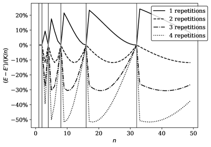
Figure 12: Difference in expected number of keys

Taking the hanging tree in Fig. 8, the valid nodes are those in range $[0,10]$. Nodes from $8$ to $10$ belong to the last level, while nodes from $0$ to $7$ belong to the other levels. The probability of landing in the range $[8,10]$ is slightly different from the probability of landing in the range $[0,7]$. By repeating block $B$ multiple times (with a different hash), the probability of sending keys in the range $[8,10]$ will increase (Fig. 12 shows the distribution of keys for different repetitions of block $B$).

In a perfectly balanced system, we expect every node to get $\frac{k}{n}$ keys. As detailed in Sec.V-E and Sec.V-F, we can obtain the best behavior applying block $B$ up to two times. Applying the central block a different number of times always leads to an unbalanced distribution.

IV-A Relocation function

Also, the relocation function is implemented by leveraging binary arithmetic principles. As delineated in Prop. III.10, when a b-array is represented as a hanging tree, for every level $l$, the value of the leftmost node of $l$ is $2^{l-1}$, and the capacity of level $l$ is also $2^{l-1}$. The binary representation of a numerical value $x$ is articulated as follows:

$$x=x_{0}\cdot 2^{0}+x_{1}\cdot 2^{1}+x_{2}\cdot 2^{2}+x_{n-1}\cdot 2^{n-}1+x_{n}\cdot 2^{n}$$ (1)

where, $n\geq 0$ and $\forall i,x_{i}\in\{0,1\}$. Consequently, it is evident that, given a specific bucket $b$, its depth is determined by the index of the highest $1$ bit within the binary representation of $b$, and correspondingly, the level of $b$ is determined by its depth incremented by one, as per Def. III.4. For instance, considering the bucket $11$ as an illustrative example, its binary representation is depicted as:

$$11=1\cdot 2^{0}+1\cdot 2^{1}+0\cdot 2^{2}+1\cdot 2^{3}.$$

Thus, the depth of bucket $b$ is $3$, positioning it within level $4$ as exemplified in Fig. 8. Algorithm 2 provides a possible implementation of the relocation function.

Algorithm 2 Relocate within level

1:function relocateWithinLevel($b$, $h$)

2:     if $b<2$ then

3:         return $b$

4:     end if

5:     $d\leftarrow highestOneBitIndex(b)$

6:     $f\leftarrow 2^{d}-1$

7:     $r\leftarrow hash(h,f)$

8:     $i\leftarrow r\ \mathtt{AND}\ f$

9:     return $d+i$

10:end function

According to Note III.12, we treat level $0$ as a special case. Moreover, since level $1$ counts only one node, we do not need to perform any relocation. Therefore, if the bucket is $0$ or $1$, belonging to either level $0$ or level $1$, we return it as it is (Alg. 2, lines $2$ and $3$). Otherwise, we compute its depth $d$ by finding the index of the highest $1$ bit. We create a bit mask $f=2^{d}-1$ that will map any number into a value in the range $[0,2^{d}-1]$ if used in combination with the bitwise $\mathtt{AND}$ operator.

V Analysis

In this section we formally prove the properties of the algorithm. We assume the looked up keys to be bounded in size. Therefore, we assume the underlying hash function to execute in constant time. Given this assumption, it is trivial to see that Algorithm 1 executes in constant time. It is also trivial to see that the algorithm occupies a minimal amount of space.

V-A Monotonicity

In this section, we will prove that monotonicity holds for BinomialHash. The property of monotonicity states that when a new bucket is added, keys only move from an existing bucket to the new one, but not between existing ones. We will prove this property by induction on the number of buckets $n$.

• n=1: the property trivially holds for $n=1$; keys can only move from the single existing bucket to the new one.

• n: we assume the property holds for $n\geq 1$.

• L¡n¡U: when a new node joins the cluster, keys initially mapped to buckets in the range $[0,n\!-\!1]$ by block $A$ will keep their positions, since the mapping only depends on the key and on $U$. A fraction $\frac{k}{U}$ of the keys will be assigned to bucket $n$ by block $A$. For the remaining keys, those mapped to the range $[L,n\!-\!1]$ by block $B$ will keep their positions, since the assignment only depends on the key and on $U$. Finally, block $C$ only maps keys in the range $[0,L\!-\!1]$. Since neither $L$ nor $U$ change when $L<n<U$ and a new node joins the cluster, keys either keep their position or move to the new bucket $n$.

• n=U: when $n=U$ all the available buckets in the upper tree are valid. The keys are uniformly distributed among the $U$ valid buckets by block $A$ of the algorithm. Since all buckets are valid the other blocks are not executed. To add a new bucket, we must also add a new level of the tree. Therefore, the current upper tree becomes the new lower tree and the new upper tree will have twice the size of the current one. The boundaries of the new tree are $L^{\prime}=U$ and $U^{\prime}=2U$ and the new size of the cluster is $n+1=U+1=L^{\prime}+1$. In the new configuration, the block $A$ of the algorithm distributes half of the keys in the range $[0,L^{\prime}\!-\!1]$ and $\frac{k}{U^{\prime}}$ keys in the bucket $L^{\prime}$. The block $B$ further populate bucket $L^{\prime}$ while block $C$ distributes the remaining keys is range $[0,L^{\prime}\!-\!1]$. The results obtained from lines $4$ and $19$ of the algorithm are congruent, meaning that line $4$ applied to $U$ and line $19$ applied to $L^{\prime}$ distribute the keys in the exact same way. Therefore, keys either keep their position or move to the new bucket $L^{\prime}$.

V-B Minimal disruption

In this section, we will prove that minimal disruption holds for BinomialHash. The property of minimal disruption states that when a bucket is removed, only the keys previously mapped to that bucket should move to a new location. We will prove this property by induction on the number of buckets $n$.

• n=2: the property trivially holds for $n=2$; when we remove a node, keys can only move from the removed bucket to the single remaining bucket.

• n-1: we assume the property holds for $n\!-\!1\geq 2$.

• n=L+1: when $n=L+1$ the last level of the tree contains only one valid node. The block $A$ of the algorithm distributes half of the keys in the range $[0,L\!-\!1]$ and $\frac{k}{U}$ keys in the bucket $L$. The block $B$ further populate bucket $L$ while block $C$ distributes the remaining keys is range $[0,L\!-\!1]$. When we remove bucket $L$, we must remove the last level of the tree. Therefore, the current lower tree becomes the new upper tree and the new lower tree will have half the size of the current one. The boundaries of the new tree are $U^{\prime}=L$ and $L^{\prime}=\frac{L}{2}$ and the new size of the cluster is $n-1=L=U^{\prime}$. In the new configuration, the keys are uniformly distributed among the $U^{\prime}$ valid buckets by block $A$ of the algorithm. Since all buckets are valid the other blocks are not executed. The results of lines $4$ and $19$ of the algorithm are congruent, meaning that line $4$ applied to $U^{\prime}$ and line $19$ applied to $L$ distribute the keys in the exact same way. Therefore, keys previously mapped to buckets in the range $[0,L-1]$ keep their positions, while keys previously mapped to bucket $L$ are distributed among the valid nodes.

• L+1¡n¡U: given a cluster of size $n+1$, when bucket $n$ leaves the cluster, keys initially mapped to buckets in the range $[0,n\!-\!1]$ by block $A$ will keep their positions. For the remaining keys, those mapped to the range $[L,n\!-\!1]$ by block $B$ will keep their positions. Block $C$ only maps keys in the range $[0,L-1]$. Therefore, keys previously mapped to buckets in the range $[0,n-1]$ keep their positions, while keys previously mapped to bucket $n$ are distributed among the valid nodes.

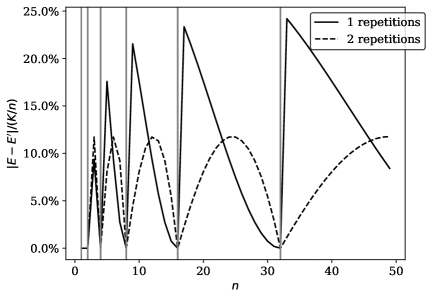
Figure 13: Absolute difference in expected number of keys, detail with 1 and 2 repetitions: the intersection between the two plots corresponds to the switch point $n_{\star}\approx 1.44\cdot L$

V-C Balance

Let us call $r$ the number of iterations in the for loop in block $B$. In this section, we will provide an upper bound for the key balance and advocate the choice $r=2$ for our algorithm by characterising the probability distribution over the keys obtained for a generic $r$. Let $n$ denote the number of buckets and $l$ the smallest positive integer such that $n\leq 2^{l}$. Accordingly, $2^{l-1}$ is the number of buckets in the lower tree (range $[0,2^{l-1}-1]$) and $2^{l}$ is the number of buckets in the upper tree. For $n=2^{l}$, by construction, we have a perfect balance over the keys. Thus, in the following, we only focus on the case $n<2^{l}$. Our goal is to minimize the difference between the expected number $E$ of keys assigned to a bucket $b$, with $b<{2^{l-1}}$, and the expected number $E^{\prime}$ of keys assigned to a bucket $b^{\prime}$, with $2^{l-1}<b^{\prime}<n$. For the sake of light notation, as in Prop. IV.2, we set $L:=2^{l-1}$.

V-D Applying $r$ times the central block

Given an input key, the algorithm’s output is a valid bucket in the $[0,n-1]$ range. The procedure assigns a key to a bucket in the lower tree (buckets $b<L$) either in the first step (lines $2$ to $6$) or in the last step (lines $15$ and $16$). In the first case, we know that the value of $c$ at line $5$ is uniformly distributed across the range $[0,2L-1]$. Hence, the probability of getting the key assigned in the first step is ${n}\over{2L}$. The probability that a bucket $b$ in the lower tree gets the key at that point is $\frac{L}{2L}=\frac{1}{2}$, and the probability that a bucket $b^{\prime}$ in the last level gets the key is instead $\frac{n-L}{2L}$.

The remaining probability, i.e., $\frac{2L-n}{2L}$, corresponds to the algorithm continuing to the central block, where rehashing the key at line $9$ draws a uniformly distributed value in the range $[0,2L]$. If we obtain one of the $n-L$ buckets at the last level (out of $2L$ possible values), the function ends (line $11$). We can execute the central block $r$ times without getting a bucket at the last level with a probability $\left(1-\frac{n-L}{2L}\right)^{r}$ and reach line $13$. At line $14$, we obtain a bucket $b$ in the lower tree with probability one. Thus, the probability to get a bucket $b$ in the lower tree is:

$$\begin{split}P(b<L)&=\underbrace{\frac{1}{2}}_{\textrm{First step}}+\underbrace{~{}\frac{2L-n}{2L}}_{\textrm{Central block}}\overbrace{\left(1-\frac{n-L}{2L}\right)^{r}}^{\textrm{r repetitions}}\underbrace{1}_{\textrm{Line 14}}\end{split}\,.$$ (2)

The probability of getting to a valid bucket $b^{\prime}$ in the last level (i.e., $L\leq b^{\prime}<n$) is obtained by the normalisation of the probabilities, i.e.,

$$P(L\leq b^{\prime}<n)=1-P(b<L)\,,$$ (3)

where $P(b<L)$ is defined in Eq. (2).

If $k$ denotes the total number of keys, the expected number of keys per node in a perfectly balanced situation should be $\frac{k}{n}$. In the lower tree, such an expected number is instead:

$$E:=\frac{P(b<L)}{L}k\,,$$ (4)

where the probability in Eq. (2) has been uniformly split over the $L$ nodes and then multiplied by $k$ to obtain the expectation. By similar considerations, for the last level:

$$E^{\prime}:=\frac{P(L\leq b^{\prime}<n)}{n-L}k\,,$$ (5)

where the probability is defined as in Eq. (3).

V-E Optimal number of repetitions of the central block

We can use Eqs. (4) and (5), together with Eqs. (2) and (3), to check that $E\geq E^{\prime}$ for both $r=0$ and $r=1$. This means that, with zero or one execution of the central block, buckets in the lower tree are favoured (i.e., more keys end up in those nodes). Moreover, the imbalance is higher for $r=0$ than $r=1$ irrespectively of $n$. Further increasing the number of executions favours the valid buckets in the last level. Indeed, we can check that, for each $r\geq 2$, $E^{\prime}\geq E$ and the additional applications of the central block increase the level of imbalance (towards the last level).

Given $n\in]L,2L[$, we can regard both $E$ and $E^{\prime}$ as functions of $r$ and find that these two expectations are equal for:

$$r^{*}(n):=\frac{\log{\left(\frac{L}{n}\right)}}{\log{\left(\frac{3L-n}{2L}\right)}}\,.$$ (6)

By simple algebra, we can see that $r^{*}(n)$ is a monotonically decreasing function of $n$ and $1<r^{*}(n)<2$. This implies that $r^{*}(n)$ is not an integer number and, thus, no strategy based on our algorithm can achieve a perfect balance, no matter what $r$. Yet, we already noticed that $r=0$ provides more imbalance towards the lower tree than $r=1$ and, analogously, any $r>2$ provides more imbalance towards the last level than $r=2$. We, therefore, conclude that to minimise the imbalance in the algorithm, we only need to choose between $r=1$ or $r=2$ for any value of $n$.

V-F Determining the best value for $r$

Let us characterise the imbalance in terms of the absolute value of the difference between the expected number of keys assigned to the nodes, respectively, in the lower tree and in the last level, normalised by the expected number of keys in a node with a perfectly balanced situation, i.e.,

$$\Delta(n,r):=\frac{|E^{\prime}-E|}{\frac{k}{n}}\,.$$ (7)

An analytical expression of $\Delta(n,r)$ can be obtained from Eqs. (4) and (5), together with Eqs. (2) and (3). For $r=1$, Eq. (7) rewrites as:

$$\Delta(n,r=1)=\frac{n(2L-n)^{2}}{4L^{3}}\,,$$ (8)

while, for $r=2$, we have instead:

$$\Delta(n,r=2)=\frac{n(n-L)(2L-n)(4L-n)}{8L^{4}}\,.$$ (9)

Introducing the normalised variable $m:=\frac{n}{2L}$, we can express both the functions in Eqs. (8) and (9) as polynomials of $m$ with coefficients independent of $L$. This implies that the maxima of these functions are also independent of $L$.

In particular, for $r=1$, we have a monotonically decreasing function of $n$ going to zero for $n\to 2L$ and such that:

$$\Delta(n,r=1)\leq\lim_{n\to L}\Delta(n,r=1)=0.25\,.$$ (10)

For $r=2$, instead, the function goes to zero for both $n\to L$ and $n\to 2L$, and has a single maximum, corresponding to a root of a polynomial of degree tree of approximate $n_{\star}\simeq 1.5309L$, giving the following bound:

$$\Delta(n,r=2)\leq\Delta(n_{\star},r=2)\simeq 0.118\,.\,$$ (11)

for each $n\in]L,2L[$.

As the bound in Eq. (11) is tighter than the one in Eq. (10), $k=2$ is the choice providing the best balance while also preserving monotonicity.

An alternative to the imbalance measure in Eq. (7) could be provided by the sum of the absolute values of the differences between the two expectations and the expectation in the perfectly balanced case with the same normalization, i.e.,

$$\frac{|E-\frac{k}{n}|+|E^{\prime}-\frac{k}{n}|}{\frac{k}{n}}\,.$$ (12)

Yet, in practice, we have $E<\frac{k}{n}<E^{\prime}$ or $E^{\prime}<\frac{k}{n}<E$, and the descriptor in Eq. (12) coincides with the one in Eq. (7). We can therefore regard Eq. (12) as an additive decomposition of $\Delta(n,r)=\Gamma(n,r)+\Gamma^{\prime}(n,r)$ with two terms associated with, respectively, the nodes in the lower tree and those in the last level, i.e.,

$$\Gamma(n,r) := \frac{|E-\frac{k}{n}|}{\frac{k}{n}}$$ (13)

$$\Gamma^{\prime}(n,r) := \frac{|E^{\prime}-\frac{k}{n}|}{\frac{k}{n}}$$ (14)

For $r=2$, we already proved $E^{\prime}\geq E$ and hence $E^{\prime}\geq\frac{k}{n}\geq E$. This implies:

$$\Gamma^{\prime}(n,2)\geq\Gamma(n,2)\,,$$ (15)

for each $n\in]L,2L[$. To find The maximum relative difference from the uniform, we can therefore focus on the nodes of the last level and find the maximum of $\Gamma^{\prime}(n,2)$. This is achieved for:

$$n^{\prime}:=\frac{7-\sqrt{7}}{3}L\simeq 1.451L\,,$$ (16)

and gives the following bound:

$$\Gamma^{\prime}(n,2)\leq\Gamma^{\prime}(n^{\prime},2)=\frac{7\sqrt{7}-10}{108}\simeq 0.078$$ (17)

for each $n\in]L,2L[$. Because of Eq. (15) the bounds also holds for $\Gamma(n,2)$. In practice, the relative imbalance in the nodes of the last level is always under the $8\%$, and, a fortiori, the same also holds for the nodes of the lower tree.

VI Conclusions

In this paper, we presented a novel consistent hashing algorithm named BinomialHash, which improves upon state-of-the-art algorithms such as JumpHash[1], PowerCH[2]. We provided implementation details and theoretical guarantees. Our solution is an advancement over existing algorithms because it executes lookups in constant time $O(1)$ and maintains minimal memory usage. In contrast to Power CH[2], our algorithm is not patent encumbered. The usage scenario for BionomialHash involves scaling the cluster by adding and removing buckets in a Last-In-First-Out order. Current work focuses on extensive benchmarking (using the framework proposed in [4]) and on implementing BinomialHash as a replacement of JumpHash within MementoHash[5].

References

- [1] J. Lamping and E. Veach, “A fast, minimal memory, consistent hash algorithm,” arXiv preprint arXiv:1406.2294, 2014.
- [2] E. Leu, “Fast consistent hashing in constant time,” 2023.
- [3] T. H. Cormen, C. E. Leiserson, R. L. Rivest, and C. Stein, Introduction to algorithms. MIT press, 2022.
- [4] M. Coluzzi, A. Brocco, and T. Leidi, “Consistently faster: A survey and fair comparison of consistent hashing algorithms,” in Proceedings of SEBD 2023: 31st Symposium on Advanced Database System, July 02–05, 2023, Galzignano Terme, Padua, Italy, ser. CEUR Workshop Proceedings, 2023.
- [5] M. Coluzzi, A. Brocco, A. Antonucci, and T. Leidi, “Mementohash: A stateful, minimal memory, best performing consistent hash algorithm,” ArXiv, vol. abs/2306.09783, 2023. [Online]. Available: https://api.semanticscholar.org/CorpusID:259187732