Meshfree Variational Physics Informed Neural Networks (MF-VPINN): an adaptive training strategy

Abstract

In this paper we introduce a Meshfree Variational Physics Informed Neural Network. It is a Variational Physics Informed Neural Network that does not require the generation of a triangulation of the entire domain and that can be trained with an adaptive set of test functions. In order to generate the test space we exploit an a posteriori error indicator and add test functions only where the error is higher. Four training strategies are proposed and compared. Numerical results show that the accuracy is higher than the one of a Variational Physics Informed Neural Network trained with the same number of test functions but defined on a quasi-uniform mesh.

Keywords VPINN; Meshfree; Physics-Informed Neural Networks; Error estimator; Patches

MSC-class 65N12; 65N15; 65N50; 68T05; 92B20

1 Introduction

Physics Informed Neural Networks (PINNs) are a rapidly emerging numerical technique to solve Partial Differential Equations (PDEs) by means of a deep neural network. The first idea can be traced back to the works of Lagaris et al. [16, 17, 18] but, thanks to the hardware advancements and the existence of deep learning packages like Tensorflow [1] and Pytorch [20], they recently become popular after the works of Raissi et al. [23, 24], published in [25]. In its original formulation, the approximate solution is computed as the output of a neural network trained to minimize the PDE residual on a set of collocation points inside the domain and on its boundary.

The growing interest in PINNs is strictly related to their flexibility. In fact, with minor changes to the implementation, it is possible to solve a huge variety of problems. For example, exploiting the nonlinear nature of the involved neural network, nonlinear [22, 34] and high-dimensional [11] PDEs can be solved without the need for globalization methods or additional nonlinear solvers. Moreover, changing the neural network input dimension or suitably adapting the loss function, it is possible to solve parametric [9, 10] or inverse [36, 28] problems. When external data are available, they can also be used to guide the optimization phase and improve the PINN accuracy [7].

In order to improve the original PINN proposed in [25] and to adapt it to solve specific problems, several generalizations have been proposed. For example, in the Deep Ritz Method (DRM) [30] one looks for a minimizer of the PDE energy functional, in the Deep Galerkin Method (DGM) [26] an approximation of the $L^{2}$ norm of the PDE residual is minimized, and, in the Variational Physics Informed Neural Network (VPINN) [13, 14] the weak formulation of the problem is used to construct the loss function. It is also possible to exploit domain decomposition strategies and enforce flux continuity on the subdomain interfaces as in the Conservative PINN (CPINN) [12] or to change the neural network architecture or the training strategy as in [10, 29, 32, 33, 35, 37]. More extensive overviews of the existing approaches can be found in [3, 8, 19].

In this work we focus on VPINNs. As discussed in [4, 5, 13, 14], in order to train a VPINN, one needs to choose a suitable space of test functions, compute the variational residuals against all the test functions in a basis of such a space and minimize a linear combination of these residuals. We highlight that the PDE variational formulation is required in presence of discontinuous physical coefficients or singular forcing terms. However, one of the VPINN limitations is that a triangulation of the entire domain is required to define the test functions, generating it may be very expensive or even impractical for moderate or high-dimensional problems. In this work we present a Meshfree VPINN (MF-VPINN) that does not require a global triangulation of the domain but is trained with the same loss function and neural network architecture of a standard VPINN.

The paper is organized as follows. In Sect. 2 we introduce the problem we are interested in. In particular, we focus on the problem discretization in Sect. 2.1 and on the MF-VPINN loss function in Sect 2.2. Then, an a posteriori error estimator is presented in Sect. 2.3 and used in Sect. 2.4 to iteratively generate the required test functions. Numerical results are presented in Sect. 3. In Sect. 3.1 we describe the model implementation and some strategies to improve the model efficiency, in Sect. 3.2 we compare different approaches to generate the test functions and compare their performance and, in Sect. 3.3, we analyze the role of the error estimator introduced in Sect. 2.3. Finally, we conclude the paper in Sect. 4 and discuss future perspectives and ideas.

2 Problem formulation

Let us consider the following second-order elliptic problem, defined on a polygonal or polyhedral domain $\Omega\subset{\mathbb{R}}^{n}$ with Lipshitz boundary $\Gamma=\partial\Omega$:

$$\begin{cases}Lu:=-\nabla\cdot(\mu\nabla u)+\bm{\beta}\cdot\nabla u+\sigma u=f&\text{in \ }\Omega\,,\\ u=g&\text{on \ }\Gamma\,,\end{cases}$$ (2.1)

where $\mu,\sigma\in{\rm L}^{\infty}(\Omega)$, $\bm{\beta}\in({\rm W}^{1,\infty}(\Omega))^{n}$ satisfy $\mu\geq\mu_{0}$, $\sigma-\frac{1}{2}\nabla\cdot\bm{\beta}\geq 0$ in $\Omega$ for some constant $\mu_{0}>0$, whereas $f\in L^{2}(\Omega)$ and $g=\bar{u}_{|\Gamma}$ for some $\bar{u}\in{\rm H}^{1}(\Omega)$.

In order to derive the corresponding variational formulation, we define the bilinear form $a$ and the linear form $F$ as:

$$a:V\times V\to\mathbb{R}\,,\qquad a(w,v)=\int_{\Omega}\mu\nabla w\cdot\nabla v+\bm{\beta}\cdot\nabla w\,v+\sigma w\,v\,,$$ (2.2)

$$F:V\to\mathbb{R}\,,\qquad F(v)=\int_{\Omega}f\,v\,;$$ (2.3)

where $V$ is the function space $V=H_{0}^{1}(\Omega)$. We denote by $\alpha\geq\mu_{0}$ the coercivity constant of $a$ and by $\|a\|$ and $\|F\|$ the continuity constants of $a$ and $F$. Then, the variational formulation of Problem (2.1) reads as: Find $u\in\bar{u}+V$ such that

$$a(u,v)=F(v)\qquad\forall v\in V\,.$$ (2.4)

2.1 Problem discretization

In order to numerically solve problem (2.4), one needs to choose suitable finite-dimensional approximations of the trial space $\bar{u}+V$ and of the test space $V$. A Galerkin formulation is considered when the two discrete spaces coincide, whereas a Petrov-Galerkin formulation is considered otherwise. In this work we consider a Petrov-Galerkin formulation, in which the trial space is approximated by a set of functions $V^{\mathcal{NN}}$ represented by a neural network, suitably modified to enforce the Dirichlet boundary conditions, and the test space is a space $V_{h}$ of piecewise linear functions.

The neural network considered in the following is a standard fully-connected feed-forward neural network. Given the number $L$ of layers and a set of matrices $A_{\ell}\in\mathbb{R}^{N_{\ell}\times N_{\ell-1}}$ and vectors $b_{\ell}\in\mathbb{R}^{N_{\ell}}$, $\ell=1,...,L$ containing the neural network trainable weights, the function $w:{\mathbb{R}}^{n}\rightarrow{\mathbb{R}}$ associated with the considered neural network architecture is:

$$x_{0}=\bm{x},$$ (2.5)

$$x_{\ell}=\rho(A_{\ell}x_{\ell-1}+b_{\ell}),\hskip 28.45274pt\ell=1,...,L-1,$$

$$w(\bm{x})=A_{L}x_{L-1}+b_{L}.$$

Here $\rho:{\mathbb{R}}\rightarrow{\mathbb{R}}$ is a nonlinear function element-wise applied to the vector $A_{\ell}x_{\ell-1}+b_{\ell}$. In this chapter we use $\rho(x)=\tanh(x)$, other common choices include, but are not limited to, $\rho(x)=\text{ReLU}(x)=\max\{0,x\}$, $\rho(x)=\text{RePU}(x)=\max\{0,x^{p}\}$ for $1<p\in{\mathbb{N}}$, $\rho(x)=1/(1+e^{-x})$ and $\rho(x)=\log(1+e^{x})$. Note that, in order to represent a function $w:{\mathbb{R}}^{n}\rightarrow{\mathbb{R}}$, the layer widths $N_{\ell}$ of the first and last layers are chosen as $N_{0}=n$ and $N_{L}=1$. We denote by $W^{\mathcal{NN}}$ the set of functions that can be represented as in (2.5) for any combination of the neural network weights and by ${\bm{w}}^{\mathcal{NN}}$ the vector containing all the trainable weights of the neural network.

The function $w$ defined in (2.5) is independent of the differential problem that has to be solved and is, in most of the papers on PINNs or related models, trained to minimize both the residual of the equation and a term penalizing the discrepancy between $w_{|\Gamma}$ and $g$. Instead, we add a non-trainable layer $B$ to the neural network architecture in order to automatically enforce the required boundary conditions without the need to learn them during the training. As described in [27], the operator $B$ acts on the neural network output as:

$$Bw=\phi w+\bar{g},$$ (2.6)

where $\phi:\Omega\rightarrow{\mathbb{R}}$ is a function vanishing on $\Gamma$ and strictly positive inside $\Omega$, and $\bar{g}:\Omega\rightarrow{\mathbb{R}}$ is a suitable extension of $g:\Gamma\rightarrow{\mathbb{R}}$. The advantages of such an approach are also described in [6]. Then, the discrete trial space approximating $\bar{u}+V$ can be defined as:

$$V^{\mathcal{NN}}=\{v^{\mathcal{NN}}\in\bar{u}+V:v^{\mathcal{NN}}=Bw\text{ for some }w\in W^{\mathcal{NN}}\}\,.$$

On the other hand, the discrete test space $V_{h}$ is not associated with the neural network and only contains known test functions. In standard VPINNs, one generates a triangulation $\cal{T}$ of the domain $\Omega$ and then defines $V_{h}$ as the space of functions that coincide with a polynomial of order $p\in{\mathbb{N}}$ inside each element of $\cal{T}$. Instead, we want to construct a discrete space $V_{h}$ of functions independent from a global triangulation $\cal{T}$. Moreover, since in [5] it has been proven that the VPINN convergence rate with respect to mesh refinement decreases when the order of the test functions is increased, we are interested in a space $V_{h}$ that only contains piecewise linear functions. For the sake of simplicity we only consider the case $n=2$, the discussion can be directly generalized to the more general case $n\in{\mathbb{N}}$.

Let $\hat{P}\subset{\mathbb{R}}^{n}$ be a reference patch. In the following discussion $\hat{P}$ can be any arbitrary star-shaped polygon with $N_{\hat{P}}$ vertices and the dimension of its kernel strictly greater than zero. Nevertheless, in the numerical experiments we only consider the reference patch $\hat{P}=[0,1]^{2}$ to avoid any unnecessary computational overhead. Let ${\cal{M}}=\{M_{i}\}_{i=1}^{n_{\text{patches}}}$ be a set of affine mappings such that $M_{i}:\hat{P}\rightarrow P_{i}\subset\Omega$, where we denote as $P_{i}$ the patch obtained transforming the reference patch $\hat{P}$ through the map $M_{i}$. We assume that ${\cal P}=\{P_{i}\}_{i=1}^{n_{\text{patches}}}$ is a cover of $\Omega$, i.e. $\cup_{i=1}^{n_{\text{patches}}}P_{i}=\Omega$, and we admit overlapping patches.

Let us consider the triangulation $\hat{\cal{T}}=\{\hat{T}_{j}:1\leq j\leq N_{\hat{P}}\}$ of $\hat{P}$ obtained connecting each vertex with a single point $\bm{c}_{\hat{P}}$ in its kernel. It is then possible to define a piecewise linear function $\hat{\varphi}$ vanishing on the border of $\hat{P}$ and such that $\hat{\varphi}(\bm{c}_{\hat{P}})=1$ and $\hat{\varphi}_{|\hat{T}_{j}}\in{\mathbb{P}}_{1}(\hat{T}_{j})$, for any $j=1,\dots,N_{\hat{P}}$. Then, we define the discrete test space $V_{h}$ as $V_{h}=\text{span}\{\varphi_{i}:i=1,\dots,n_{\text{patches}}\}$, where $\varphi_{i}\in V$ is the piecewise linear function:

$$\varphi_{i}(\bm{x})=\begin{cases}\hat{\varphi}(M_{i}^{-1}(\bm{x})),&\bm{x}\in P_{i},\\ 0,&\bm{x}\notin P_{i}.\end{cases}$$ (2.7)

We remark that the only required triangulation is $\hat{\cal{T}}$, which contains only $N_{\hat{P}}$ triangles (in the numerical tests in this paper $N_{\hat{P}}=4$). Instead, there exists no mesh on $\Omega$ and the test functions $\varphi_{i}$ and their supports $P_{i}$ are all independent. Therefore, the proposed method is said to be meshfree. A simple example of a set of patches ${\cal P}$ with $n_{\text{patches}}=7$ on the domain $\Omega=[0,1]^{2}$ is shown in Fig. 1. For the sake of simplicity, in this work we consider a squared reference patch $\hat{P}$ with $\bm{c_{\hat{P}}}$ coinciding with its center, and let each mapping $M_{i}$ represent a combination of scalings and translations.

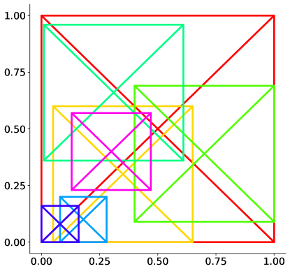
Figure 1: Graphical representation of a set $\{P_{i}\}_{i=1}^{n_{\text{patches}}}$ obtained from a squared reference patch $\hat{P}$ with $\bm{c_{\hat{P}}}$ in its center covering the domain $\Omega=(0,1)^{2}$.

Using the introduced finite-dimensional set of functions $V^{\mathcal{NN}}$ and $V_{h}$, it is possible to discretize problem (2.4) as follows: Find $u^{\mathcal{NN}}\in V^{\mathcal{NN}}$ such that

$$a(u^{\mathcal{NN}},v)=F(v)\qquad\forall v\in V_{h}\,.$$ (2.8)

2.2 Loss function

In this section we derive the loss function used to train the neural network. It has to be computable and its minimizer has to be an approximate solution of problem (2.4).

Let us consider a quadrature rule of order $q\geq 2$ on each triangle $T_{j}\in\hat{\cal{T}}$, $j=1,\dots,N_{\hat{P}}$, uniquely identified by a set of nodes and weights $\{(\widetilde{\bm{\xi}}^{j}_{\ell},\widetilde{\omega}^{j}_{\ell}):\ell\in I^{T_{j}}\}$. The nodes and weights of a composite quadrature formula of order $q$ on $\hat{P}$ can be obtained as

$$\{(\hat{\bm{\xi}}_{\ell},\hat{\omega}_{\ell}):\ell\in I^{\hat{P}}\}=\bigcup_{j=1}^{N_{\hat{P}}}\{(\widetilde{\bm{\xi}}^{j}_{\ell},\widetilde{\omega}^{j}_{\ell}):\ell\in I^{T_{j}}\}.$$

Then, the corresponding quadrature rule of order $q$ of an arbitrary patch $P_{i}$ is defined as:

$$\left\{(\bm{\xi}^{i}_{\ell},\omega^{i}_{\ell}):\ell\in I^{\hat{P}}|\bm{\xi}^{i}_{\ell}=M_{i}(\hat{\bm{\xi}}_{\ell}),\omega^{i}_{\ell}=\hat{\omega}_{\ell}\dfrac{\text{area}(P_{i})}{\text{area}(\hat{P})}\right\}.$$ (2.9)

Using the quadrature rule in (2.9), it is possible to define an approximate restriction on each patch of the forms $a$ and $F$ as follows:

$$a_{h}^{i}(w,v)=\sum_{\ell\in I^{\hat{P}}}[\mu\nabla w\cdot\nabla v+\bm{\beta}\cdot\nabla w\,v+\sigma wv](\bm{\xi}^{i}_{\ell})\,\omega^{i}_{\ell}\approx a_{P_{i}}(w,v)\,,$$ (2.10)

$$F_{h}^{i}(v)=\sum_{\ell\in I^{\hat{P}}}[fv](\bm{\xi}^{i}_{\ell})\,\omega^{i}_{\ell}\approx F_{P_{i}}(v)\,,$$ (2.11)

where $a_{P_{i}}(w,v)$ and $F_{P_{i}}(v)$ are defined as in (2.2) and (2.3) but restricting the supports of the integrals to $P_{i}$. We remark that, since it is not possible to compute integrals involving a neural network exactly, we can only use the forms $a_{h}^{i}$ and $F_{h}^{i}$ in the loss function. Exploiting the linearity of $a(w,v)$ and $F(v)$ with respect to $v$ to consider only the basis $\{\varphi_{i}\}_{i=1}^{n_{\text{patches}}}$ of $V_{h}$ as set of test functions, we approximate problem (2.8) as: Find $u^{\mathcal{NN}}\in V^{\mathcal{NN}}$ such that

$$a_{h}^{i}(u^{\mathcal{NN}},\varphi_{i})=F_{h}^{i}(\varphi_{i})\qquad\forall i=1,\dots,n_{\text{patches}}\,.$$ (2.12)

Then, in order to cast problem (2.12) into an optimization problem, we define the residuals

$$r_{h,i}(w)=F_{h}^{i}(\varphi_{i})-a_{h}^{i}(w,\varphi_{i})\,,\qquad i=1,\dots,n_{\text{patches}}$$ (2.13)

and the loss function

$$R_{h}^{2}(w;{\cal P})=\dfrac{1}{n_{\text{patches}}}\sum_{i=1}^{n_{\text{patches}}}\gamma_{i}r_{h,i}^{2}(w)\,,$$ (2.14)

where $\gamma_{i}$ are suitable positive scaling coefficients. In this work we use $\gamma_{i}=\text{area}(P_{i})^{-1}$ to give the same importance to each patch. Note that this is equivalent to normalizing the quadrature rules involved in (2.10) and (2.11); this way each residual $r_{h,i}$ can be regarded as a linear combination of the MF-VPINN value and derivatives independent of the size of the support of the patch $P_{i}$. We also highlight that the loss function depends on the choice of $\cal M$ since all the used test functions are generated starting from the corresponding mappings $M_{i}\in\cal M$. We are now interested in a practical procedure to obtain a set $\widetilde{\cal P}$ such that the approximate solution computed minimizing $R_{h}^{2}(\cdot;\widetilde{\cal P})$ is as accurate as possible with $\widetilde{\cal P}$ as small as possible.

2.3 The a posteriori error estimator

The goal of this section is to derive an error estimator associated with an arbitrary patch $P_{i}$, with $i\in\{1,\dots,n_{\text{patches}}\}$. To do so, we rely on the a posteriori error estimator proposed in [4]. It has been proven to be efficient and reliable, therefore, such an estimator allows us to know where the error is larger without knowing the exact solution of the PDE. Let us consider the patch $P_{i}$, formed by the triangles $T_{i,1},\dots,T_{i,N_{\hat{P}}}$ and a triangulation ${\cal T}_{i}$ of $\Omega$ such that $T_{i,j}\in{\cal T}_{i}$, for every $j=1,\dots,N_{\hat{P}}$. We remark that the triangulation ${\cal T}_{i}$ does not have to be explicitly generated, it is only used to properly define all the quantities introduced in [4] required to derive the proposed error estimator.

Let $V_{h}^{i}=\text{span}\{\psi_{j}^{i}:1\leq j\leq\text{dim}\left(V_{h}^{i}\right)\}$ be the space of piecewise linear functions defined on ${\cal T}_{i}$. Where $\{\psi_{j}^{i}:1\leq j\leq\text{dim}\left(V_{h}^{i}\right)\}$ is a Lagrange basis of $V_{h}^{i}$. It is then possible to define two constants $c_{h}^{i}$ and $C_{h}^{i}$, with $0<c_{h}^{i}<C_{h}^{i}$, such that:

$$c_{h}^{i}|v|_{1,\Omega}\leq\|\bm{v}\|_{2}\leq C_{h}^{i}|v|_{1,\Omega}\qquad\forall v\in V_{h}^{i}\,,$$ (2.15)

where $v=\sum_{j=1}^{\text{dim}\left(V_{h}^{i}\right)}v_{j}\psi_{j}^{i}$ is an arbitrary element of $V_{h}^{i}$ associated with the expansion coefficients $\bm{v}=\left\{v_{1},\dots,v_{\text{dim}\left(V_{h}^{i}\right)}\right\}$ and $\|\bm{v}\|_{2}=\left(\sum_{j=1}^{\text{dim}\left(V_{h}^{i}\right)}v_{i}^{2}\right)^{1/2}$.

Then, given an integer $k\geq 0$, for any element $E\in{\cal T}_{i}$, we define the projection operator $\Pi_{E,k}:L^{2}(E)\to\mathbb{P}_{k}(E)$ such that:

$$\int_{E}\Pi_{E,k}\phi=\int_{E}\phi\qquad\forall\phi\in L^{2}(E)\,.$$ (2.16)

We also denote by $\{(\bm{\xi}_{\ell}^{E},\omega_{\ell}^{E}):\ell\in I^{E}\}$ a quadrature formula of order $q$ on $E$ and define the quadrature-based discrete seminorm:

$$\|v\|_{0,E,\omega}=\left(\sum_{\ell\in I^{E}}v^{2}(\bm{\xi}^{E}_{\ell})\,\omega^{E}_{\ell}\right)^{1/2}\,.$$ (2.17)

We require the weights and nodes of this quadrature rule to coincide with the ones introduced in (2.9) when $E$ is a triangle included in $P_{i}$ (i.e. when $E\in\{T_{i,1},\dots,T_{i,N_{\hat{P}}}\}$). We can now introduce all the terms involved in the a posteriori error estimator.

Let $\eta_{{\mathrm{rhs}},1}(E)$ and $\eta_{{\mathrm{rhs}},2}(E)$ be the quantities:

$$\begin{split}\eta_{{\mathrm{rhs}},1}(E)&=h_{E}\|f-\Pi_{E,q-1}f\|_{0,E}\,,\\[3.0pt] \eta_{{\mathrm{rhs}},2}(E)&=h_{E}\|f-\Pi_{E,q-1}f\|_{0,E,\omega}+\|f-\Pi_{E,q}f\|_{0,E,\omega}\,.\end{split}$$ (2.18)

They measures the oscillations of the forcing term with respect to its polynomial projections in various norms. Similar oscillations are also measured for the diffusion, convection and reaction terms by the terms $\eta_{{\mathrm{coef}},i}(E)$ for $i=1,\dots,6$:

$$\begin{split}\eta_{{\mathrm{coef}},1}(E)&=\|\mu\nabla u^{\mathcal{NN}}-\Pi_{E,q}(\mu\nabla u^{\mathcal{NN}})\|_{0,E}\,,\\[3.0pt] \eta_{{\mathrm{coef}},2}(E)&=h_{E}\|\bm{\beta}\cdot\nabla u^{\mathcal{NN}}-\Pi_{E,q-1}(\bm{\beta}\cdot\nabla u^{\mathcal{NN}})\|_{0,E}\,,\\[3.0pt] \eta_{{\mathrm{coef}},3}(E)&=h_{E}\|\sigma u^{\mathcal{NN}}-\Pi_{E,q-1}(\sigma u^{\mathcal{NN}})\|_{0,E}\,,\\[3.0pt] \eta_{{\mathrm{coef}},4}(E)&=\|\mu\nabla u^{\mathcal{NN}}-\Pi_{E,q}(\mu\nabla u^{\mathcal{NN}})\|_{0,E,\omega}\,,\\[3.0pt] \eta_{{\mathrm{coef}},5}(E)&=h_{E}\|\bm{\beta}\cdot\nabla u^{\mathcal{NN}}-\Pi_{E,q-1}(\bm{\beta}\cdot\nabla u^{\mathcal{NN}})\|_{0,E,\omega}\,,\\[3.0pt] &\qquad\qquad\qquad+\|\bm{\beta}\cdot\nabla u^{\mathcal{NN}}-\Pi_{E,q}(\bm{\beta}\cdot\nabla u^{\mathcal{NN}})\|_{0,E,\omega}\\[3.0pt] \eta_{{\mathrm{coef}},6}(E)&=h_{E}\|\sigma u^{\mathcal{NN}}-\Pi_{E,q-1}(\sigma u^{\mathcal{NN}})\|_{0,E,\omega}\\[3.0pt] &\qquad\qquad\qquad+\|\sigma u^{\mathcal{NN}}-\Pi_{E,q}(\sigma u^{\mathcal{NN}})\|_{0,E,\omega}\,,\end{split}$$ (2.19)

where $u^{\mathcal{NN}}$ is the output of the neural network after the enforcement of the Dirichlet boundary conditions through the operator $B$ and $h_{E}$ is the diameter of $E$. Then, let us define the term $\eta_{{\mathrm{r}es}}(E)$, that measure how well the equation is satisfied, as:

$$\eta_{{\mathrm{res}}}(E)=h_{E}\|\,{\mathrm{bulk}}_{E}(u^{\mathcal{NN}})\,\|_{0,E}+h_{E}^{1/2}\sum_{e\subset\partial E}\|\,{\mathrm{jump}}_{e}(u^{\mathcal{NN}})\,\|_{0,e}\,,$$ (2.20)

where

$${\mathrm{bulk}}_{E}(u^{\mathcal{NN}})=\Pi_{E,q-1}f+\nabla\cdot\Pi_{E,q}(\mu\nabla u^{\mathcal{NN}})-\Pi_{E,q-1}(\bm{\beta}\cdot\nabla u^{\mathcal{NN}}+\sigma u^{\mathcal{NN}})$$

$${\mathrm{jump}}_{e}(u^{\mathcal{NN}})=\Pi_{E_{1},q}(\mu\nabla u^{\mathcal{NN}})\cdot\bm{n}-\Pi_{E_{2},q}(\mu\nabla u^{\mathcal{NN}})\cdot\bm{n}\,.$$

Note that ${\mathrm{jump}}_{e}(u^{\mathcal{NN}})$ measures the interelemental jumps of $\Pi_{E,q}(\mu\nabla u^{\mathcal{NN}})$ across the edge $e$ with normal unit vector $\bm{n}$ shared by the elements $E_{1}$ and $E_{2}$.

Finally, we introduce the elemental approximate forms:

$$a_{h}^{i,E}(w,v)=\sum_{\ell\in I^{E}}[\mu\nabla w\cdot\nabla v+\bm{\beta}\cdot\nabla w\,v+\sigma wv](\bm{\xi}^{E}_{\ell})\,\omega^{E}_{\ell}\,,$$ (2.21)

$$F_{h}^{i,E}(v)=\sum_{\ell\in I^{E}}[fv](\bm{\xi}^{E}_{\ell})\,\omega^{E}_{\ell}\,,$$ (2.22)

where $\bm{\xi}^{E}_{\ell}$ and $\omega^{E}_{\ell}$, $\ell\in I^{E}$, are the nodes and weights used in equation (2.17). With such forms, it is possible to define the residuals

$$r_{h,i,j}(w)=\sum_{E\in{\cal T}_{i}}F_{h}^{i,E}(\psi_{j}^{i})-a_{h}^{i,E}(w,\psi_{j}^{i})\,,\qquad j=1,\dots,\text{dim}\left(V_{h}^{i}\right)$$

and the quantity $\eta_{\mathrm{loss}}(E)$ as:

$$\eta_{\mathrm{loss}}(E)=C_{h}\sqrt{\sum_{j\in I_{h}^{E}}r_{h,i,j}^{2}(u^{\mathcal{NN}})}\,.$$ (2.23)

Here, denoting the support of the function $\psi_{j}^{i}\in V_{h}^{i}$ by $\mathrm{supp}\,\psi_{j}^{i}$, the elemental index set

$$I_{h}^{E}=\{j\in I_{h}:E\subset{\mathrm{supp}}\,\psi_{j}^{i}\}$$

is the set containing the indices of the functions which support contains $E$. It is then possible to estimate the error between the unknown exact solution $u$ and its MF-VPINN approximation $u^{\mathcal{NN}}$ by means of the computable quantities in (2.18), (2.19), (2.20) and (2.23) as:

$$|u-u^{\mathcal{NN}}|_{1,E}\lesssim\left(\eta_{\mathrm{res}}^{2}(E)+\eta_{\mathrm{loss}}^{2}(E)+\sum_{i=1}^{6}\eta_{{\mathrm{coef}},i}^{2}(E)+\sum_{i=1}^{2}\eta_{{\mathrm{rhs}},i}^{2}(E)\right)^{1/2}\,.$$ (2.24)

Once more, we refer to [4] for the proof of such a statement.

We remind that our goal is to obtain a computable error estimator associated with a single patch $P_{i}$. When evaluated on an element $E\in P_{i}$, the quantity on the right hand side of equation (2.24) implicitly depends on several elements in $V_{h}^{i}$ that do not belong to $P_{i}$ because of the presence of $\eta_{\mathrm{res}}^{2}(E)$ and $\eta_{\mathrm{loss}}^{2}(E)$. Therefore, such an estimator is not computable without generating the triangulation ${\cal T}_{i}$ and the corresponding space $V_{h}^{i}$. Instead, we look for an error estimator that does not control the error on the entire patch but only in a neighbourhood ${\cal N}_{i}$ of its center $\bm{c_{P_{i}}}=M_{i}\left(\bm{c_{\hat{P}}}\right)$. This can be done considering only the terms whose computation involves geometric elements containing $\bm{c_{P_{i}}}$ and the only function $\psi_{j}^{i}$ that does not vanish on $\bm{c_{P_{i}}}$. Note that such a function is the function $\varphi_{i}$ defined in (2.7). Therefore, the error estimator $\eta_{i}$ that controls the error in ${\cal N}_{i}$ can be computed as:

$$\eta_{i}=\left[\eta_{\mathrm{res},i}^{2}+C_{h}^{2}r_{h,i}^{2}(u^{\mathcal{NN}})+\sum_{j=1}^{N_{\hat{P}}}\left(\sum_{k=1}^{6}\eta_{{\mathrm{coef}},k}^{2}(T_{i,j})+\sum_{k=1}^{2}\eta_{{\mathrm{rhs}},k}^{2}(T_{i,j})\right)\right]^{1/2},$$ (2.25)

where $\eta_{\mathrm{res},i}$ is defined as:

$$\eta_{{\mathrm{res}},i}=\sum_{j=1}^{N_{\hat{P}}}\left(h_{T_{i,j}}\|\,{\mathrm{bulk}}_{T_{i,j}}(u^{\mathcal{NN}})\,\|_{0,{T_{i,j}}}+h_{P_{i}}^{1/2}\|\,{\mathrm{jump}}_{e_{i,j}}(u^{\mathcal{NN}})\,\|_{0,e_{i,j}}\right)\,.$$ (2.26)

In (2.26) we denote by $h_{P_{i}}$ the diameter of the patch $P_{i}$ and by $e_{i,j},j=1,\dots,N_{\hat{P}}$ the edges connecting its vertices with $\bm{c_{P_{i}}}$.

Since $\eta_{i}$ can be seen as an approximation of the right hand side of (2.24), we use it as an indicator of the error $|u-u^{\mathcal{NN}}|_{1,{\cal N}_{i}}$. It is important to remark that $\eta_{i}$ can be computed without generating ${\cal T}_{i}$ and $V_{h}^{i}$. In fact, its computation involves only the function $\varphi_{i}$, the triangles partitioning $P_{i}$ and the edges connecting its vertices with its center.

2.4 The choice of $\cal M$ and $\cal P$

In this section the procedure adopted to generate the set of test functions used to train the MF-VPINN is described. We propose an iterative approach, in which the MF-VPINN is initially trained with very few test functions, and then other test functions are added in the regions of the domain in which the $H_{1}$ norm of the error is larger. We anticipate that, as shown in Section 3.3, generating test functions in regions where $r_{h,i}^{2}$ is large may not lead to accurate solutions because $r_{h,i}^{2}$ is not proportional to the $H_{1}$ error. Therefore, such a choice may increase the density of test functions where they are not required while maintaining only few test functions in regions in which the error is large. Instead, we use the error indicator $\eta_{i}$ defined in (2.25).

Let us initially consider a cover ${\cal P}_{0}=\{P_{i}\}_{i=1}^{n_{\text{patches}}}$ of $\Omega$ comprising few patches (i.e. $n_{\text{patches}}$ is a small integer) and the corresponding set of mappings ${\cal M}_{0}=\{M_{i}\}_{i=1}^{n_{\text{patches}}}$ and test functions $\{\varphi_{i}\}_{i=1}^{n_{\text{patches}}}$. These sets induce a loss function $R_{h}^{2}(w;{\cal P}_{0})$ as defined in (2.14), which is used to train a MF-VPINN. After this initial training, one computes $\eta_{i}^{\gamma}=\gamma_{i}\eta_{i}$ for each patch $P_{i}\in{\cal P}_{0}$ and stores the result in the array $\bm{\eta}=\left[\eta_{1}^{\gamma},\dots,\eta_{n_{\text{patches}}}^{\gamma}\right]$. Note that $\eta_{i}^{\gamma}$ is a suitable rescaling of $\eta_{i}$ to get rid of dependence from the size of $P_{i}$. Let us choose a threshold $1\leq\tau_{0}\leq n_{\text{patches}}$, sort $\bm{\eta}$ in descending order obtaining ${\bm{\eta}}_{\text{sort}}=\left[\eta_{s_{1}}^{\gamma},\dots,\eta_{s_{n_{\text{patches}}}}^{\gamma}\right]$ (where we denoted by $[s_{1},\dots,s_{n_{\text{patches}}}]$ the index set corresponding to a suitable permutation of $[1,\dots,n_{\text{patches}}]$) and consider the vector $\overline{\bm{\eta}}_{0}=\left[\eta_{s_{1}}^{\gamma},\dots,\eta_{s_{\tau_{0}}}^{\gamma}\right]$. It is possible to note that $\overline{\bm{\eta}}_{0}$ contains only the $\tau_{0}$ worst values of the indicator, it thus allows us to understand where the error is higher and where additional test functions are required to increase the model accuracy.

It is then possible to move forward with the second iteration of the iterative training. For each patch $P_{i}$ such that $\eta_{i}^{\gamma}\in\overline{\bm{\eta}}_{0}$, we generate $k_{\text{new}}$ new patches $P_{i}^{k}$, $k=1,\dots,k_{\text{new}}$ with centers inside $P_{i}$ and areas such that $\text{area}(P_{i})<\cup_{k=1}^{k_{\text{new}}}\text{area}(P_{i}^{k})<c\cdot\text{area}(P_{i})$, where $c>1$ is a tunable parameter. In the numerical experiments we use $c=1.25$. There exist different strategies to choose the number, the dimension and the position of the centers of the new patches. Such strategies are described in section 3 with particular attention to the effects of these choices on the MF-VPINN accuracy.

Let us denote by ${\cal P}_{1}$ the set ${\cal P}_{1}={\cal P}_{0}\cup\{P_{s_{1}}^{k}\}_{k=1}^{k_{\text{new}}}\cup\dots\cup\{P_{s_{\tau_{0}}}^{k}\}_{k=1}^{k_{\text{new}}}$ and by ${\cal M}_{1}$ the corresponding set of mappings. Then, it is possible to define the loss function $R_{h}^{2}(w;{\cal P}_{1})$, continue the training of the previously trained MF-VPINN, compute the error indicator $\eta_{i}^{\gamma}$ for each patch $P_{i}\in{\cal P}_{1}$ and obtain the vector $\overline{\bm{\eta}}_{1}$ used to decide where to insert the new patches to generate ${\cal P}_{2}$. In general, iterating this procedure, it is possible to compute a set of patches ${\cal P}_{m}$ and of mappings ${\cal M}_{m}$ from the previously obtained sets ${\cal P}_{m-1}$ and ${\cal M}_{m-1}$. Technical optimization details are discussed in Section 3.1.

3 Numerical results

In this section we provide several numerical results to show the performance of the training strategy described in Section 2.4. In Section 3.1 we describe the structure of the MF-VPINN implementation and highlight some details that have to be taken into account in order to increase the efficiency of the training phase. Different strategies to choose the position of the new patches are discussed in Section 3.2. The importance of the use of the error indicator is remarked in Section 3.3 with additional numerical examples.

3.1 Implementation details

The computer code used to perform the experiment is implemented in Python using the Python package Tensorflow [1] to generate the neural network architecture and train the MF-VPINN. Using the notation introduced in Section 2.1, the used neural network consists of $L=5$ layers with $N_{\ell}=50$ neurons in each hidden layer (i.e. for $\ell=1,\dots,L-1$); the activation function is the hyperbolic tangent in each hidden layer. For the first iteration of the iterative training, the neural network weights in the $\ell$-th layer are initialized with a glorot normal distribution, i.e. a truncated normal distribution with mean 0 and standard deviation equal to $\sqrt{2/(N_{\ell-1}+N_{\ell})}$. Then, for the subsequent iterations, their are initialized with the weights obtained at the end of the previous one.

During the first iteration of the training (during the minimization of $R_{h}^{2}(\cdot;{\cal P}_{0})$), the optimization is carried out exploiting the ADAM optimizer [15] with an exponentially decaying learning rate from $10^{-2}$ to $10^{-4}$ and with the second-order L-BFGS optimizer [31]. Then, from the second training iteration, we only use the L-BFGS optimizer. We remark that L-BFGS allows a very fast convergence but only if the initial starting point is close enough to the problem solution. Therefore, in the first training iteration, we use ADAM to obtain a first approximation of the solution that is then improved via L-BFGS. Then, since the $m$-th training iteration starts from the solution computed during the $(m-1)$-th one, we assume that the starting point is close enough to the solution of the new optimization problem (associated with a difference loss function with more patches) and we only use L-BFGS to increase the training efficiency.

During the $m$-th iteration of the training, the training set consists of all the quadrature nodes ${\bm{\xi}}_{\ell}^{i}$, for any $\ell\in I^{\hat{P}}$ and for any patch $P_{i}\in{\cal P}_{m}$ as defined in (2.9). The order of the chosen quadrature rule is $q=3$ inside each triangle. The Dirichlet boundary conditions are imposed by means of the operator $B$ defined in (2.6). In such operator, the function $\phi$ is a polynomial bubble vanishing on $\Gamma$ and $\overline{g}$ is the output of a neural network trained to interpolate the boundary data. To decrease the training time, the functions $\phi$, $\nabla\phi$, $\overline{g}$ and $\nabla\overline{g}$ are evaluated only once at the beginning of the $m$-th training iteration and they are then combined to evaluate $Bu^{\mathcal{NN}}$ and its gradient (where $u^{\mathcal{NN}}$ is the output of the last layer of the neural network). The derivatives of $u^{\mathcal{NN}}$ and $\overline{g}$ are computed via automatic differentiation [2] due to the complexity of their analytical expressions.

The output of the model is the value of the function $Bu^{\mathcal{NN}}$ and its gradient evaluated at the input points. Such values are then suitably combined using sparse and dense tensors to compute the quantity $R_{h}^{2}(Bu^{\mathcal{NN}};{\cal P}_{m})$. The sparse tensors contain the evaluation of $\varphi_{i}$ and $\nabla\varphi_{i}$ at each input point, whereas the dense ones store the quadrature weights, the vector $\bm{\gamma}=\{\gamma_{i}\}_{i=1}^{n_{\text{patches}}}$ and the evaluation of $\mu$, ${\bm{\beta}}$, $\sigma$ and $f$ at the input points. We highlight that all this tensors have to be computed once at the beginning of the $m$-th training iteration (updating the ones of the $(m-1)$-th iteration) to significantly decrease the training computational cost.

As discussed in Section 2.1, we assume that all the patches and test functions can be generated from a reference patch $\hat{P}$. For each patch $P_{i}\in{\cal P}_{m}$ one has to generate all the data structures required to assemble the loss function and the error indicator $\eta_{i}$. To do so, it is possible to explicitly construct all the tensors required to assemble the term ${\hat{a}}_{h}(w,\hat{\varphi})$ and all the terms involved in the computation of the reference error indicator $\hat{\eta}$ only once, at the beginning of the first iteration of the training. Then, all these tensors can be suitably rescaled to get the ones corresponding to the patches and test functions involved in the loss function and error indicators computations.

To stabilize the MF-VPINN, we introduce the $L^{2}$ regularization term

$$\mathcal{L}_{\text{reg}}({u}^{\mathcal{N\!N}})=\lambda_{\text{reg}}\|\mathbf{u}^{\mathcal{N\!N}}\|_{2}^{2},$$

where $\mathbf{u}^{\mathcal{N\!N}}$ is the set of weights of the neural network introduced in Section 2.1. In our numerical experiments we use $\lambda_{\text{reg}}=10^{-5}$. During the $m$-th iteration of the training, such a quantity is added to $R_{h}^{2}(B{u}^{\mathcal{N\!N}};{\cal P}_{m})$ to obtain the training loss function

$${\mathcal{L}}_{m}({u}^{\mathcal{N\!N}})=R_{h}^{2}(B{u}^{\mathcal{N\!N}};{\cal P}_{m})+\mathcal{L}_{\text{reg}}(\mathbf{w}^{\mathcal{N\!N}}),$$ (3.1)

that has to be minimized accurately enough. Indeed, if ${\mathcal{L}}_{m}$ is minimized poorly, the new patches ${\cal P}_{m+1}\backslash{\cal P}_{m}$ may be added in regions where they are not necessary because the accuracy of $Bu^{\mathcal{NN}}$ may still improve during the training, and may not be inserted in areas where they are required. Note that, in order to compute the numerical solution, the MF-VPINN has to be trained multiple times with different set of patches ${\cal P}_{m}$ to minimize the losses $\{{\mathcal{L}}_{m}\}$. Since such an iterative training may be expensive, we propose an early stopping strategy [21] based on the discussed error indicator to reduce its computational cost. In its basic version, early stopping consists in evaluating a chosen metric on a validation set in order to know when the neural network accuracy on data that are not present in the training set starts worsening. Interrupting the training there, prevents overfitting and improves generalization. In our context, instead, we can directly track the behaviour of the MF-VPINN $H^{1}$ error on each patch through the corresponding error indicator to understand when it stops decreasing. Therefore, given the set of patches ${\cal P}_{m}$, the chosen metric is the linear combination $ES_{m}=\sum_{i=1}^{\text{dim}({\cal P}_{m})}\eta_{i}^{\gamma}$. Numerical results showing the performance of this strategy are presented in Section 3.2.

3.2 Adaptive training strategies

Let us consider the Poisson problem:

$$\begin{cases}-\Delta u=f&\text{in \ }\Omega\,,\\ \ \ \,u=g&\text{on \ }\Gamma\,,\end{cases}$$ (3.2)

defined on the unit square $\Omega=(0,1)^{2}$. The forcing term $f$ and the boundary condition $g$ are chosen such that the exact solution is, in polar coordinates,

$$u(r,\theta)=r^{\frac{2}{3}}\sin\left(\frac{2}{3}\left(\theta+\frac{\pi}{2}\right)\right).$$ (3.3)

We use this function, represented in Fig. 2, because the solution $u$ is such that $u\in H^{5/3-\varepsilon}(\Omega)$ but $u\in C^{\infty}(\Omega\backslash{\cal N}_{0})$, where we denote by ${\cal N}_{0}$ a neighbourhood of the origin. Therefore, we know that an efficient distribution of patches has to be characterized by a high density only near the origin.

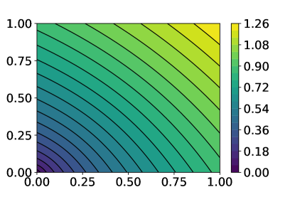
Figure 2: Graphical representation of the solution $u$ in (3.3).

Strategy #1: Random patch centers with uniform distribution

To solve problem (3.2), as a first strategy, we consider the reference patch $\hat{P}=(0,1)^{2}$ and generate a sequence of set of patches. During the first training iteration we use ${\cal P}_{0}=\{\hat{P}\}$ since this is already a cover of $\Omega$. During the second iteration we enrich the set of patches as ${\cal P}_{1}={\cal P}_{0}\cup\{P_{1},P_{2},P_{3},P_{4}\}$ where $P_{1},P_{2},P_{3}$ and $P_{4}$ are squared patches with edge $h_{i}=0.6$, $i=1,\dots,4$ and centers

$$\bm{c_{P_{1}}}=(0.3,0.3),\hskip 28.45274pt\bm{c_{P_{2}}}=(0.7,0.3),$$

$$\bm{c_{P_{3}}}=(0.3,0.7),\hskip 28.45274pt\bm{c_{P_{4}}}=(0.7,0.7).$$

This allows us to start from an homogeneous distribution of patches before utilizing the error indicator to choose the location of the new patches. Then, to decide how many patches has to be added to ${\cal P}_{m-1}$ to generate ${\cal P}_{m}$, we choose $\widetilde{\tau}_{m}$ such that:

$$\widetilde{\tau}_{m}=\text{dim}\left(\left\{\widetilde{\tau}\in\{1,\dots,\text{dim}({\cal P}_{m-1}\}:\dfrac{\sum_{i=1}^{\widetilde{\tau}}\eta_{s_{i}}^{\gamma}}{\sum_{i=1}^{\text{dim}({\cal P}_{m-1})}\eta_{i}^{\gamma}}<0.75\right\}\right)+1$$ (3.4)

and fix

$$\tau_{m}=\min(\lceil 0.3\cdot\text{dim}({\cal P}_{m-1})\rceil,\widetilde{\tau}_{m}).$$ (3.5)

Note that (3.4) allows us to consider the smallest set of patches such that the corresponding error indicators contribute at least $75\%$ of the global error indicator $ES_{m-1}$, whereas (3.5) is considered to limit the maximum number of patches that can be added for efficiency reasons.

Then, to generate the generic set of patches ${\cal P}_{m}$, we fix a multiplication factor $C_{M}$ to decide how many new patches have to be inserted inside each patch $P_{i}$ such that $\eta_{i}^{\gamma}\in\overline{\bm{\eta}}_{m-1}$. Inside each chosen patch $P_{i}$, $C_{M}$ centers $\bm{\widetilde{c}_{P_{i}^{k}}}=(\widetilde{x}_{i}^{k},\widetilde{y}_{i}^{k})$, $k=1,\dots,C_{M}$, are randomly generated with a uniform distribution and the new patches edges lengths are chosen as $h_{i}^{k}=\lambda\frac{A_{\text{ratio}}}{\sqrt{C_{M}}}h_{i}$. Here $\lambda$ is a random real value from the uniform distribution $U\left(\left[\frac{9}{10},\frac{10}{9}\right]\right)$ and the scaling coefficient $\frac{A_{\text{ratio}}}{\sqrt{C_{M}}}$ is chosen such that the sum of the areas of the new patches is $A_{\text{ratio}}$ times the area of the original patch $P_{i}$. In the numerical experiments we use $A_{\text{ratio}}=1.25$. This way, it is possible to allow the new patches to overlap and maintain the area of the region $P_{i}\backslash\left(\cup_{k=1}^{C_{M}}P_{i}^{k}\right)$ reasonably small.

We remark that, with this strategy, it may happen that some patches are outside $\Omega$. In order to avoid this risk, we move the centers $\bm{\widetilde{c}_{P_{i}^{k}}}$ to obtain the actual patches centers $\bm{c_{P_{i}^{k}}}$ as follows:

$$\bm{c_{P_{i}^{k}}}=(x_{i}^{k},y_{i}^{k})\leftarrow\left(\max\left\{\min\left\{\widetilde{x}_{i}^{k},1-\frac{h_{i}^{k}}{2}\right\},\frac{h_{i}^{k}}{2}\right\},\max\left\{\min\left\{\widetilde{y}_{i}^{k},1-\frac{h_{i}^{k}}{2}\right\},\frac{h_{i}^{k}}{2}\right\}\right).$$ (3.6)

We remark that, when the patch $P_{i}$ is very close to a vertex of the domain, it is possible that multiple original centers $\bm{\widetilde{c}_{P_{i}^{k}}}$ are such that the distance of both $\widetilde{x}_{i}^{k}$ and $\widetilde{y}_{i}^{k}$ from the $x$ and $y$ coordinates of the domain vertex is smaller than $h_{i}^{k}/2$. In this case, it is important to consider the random coefficient $\lambda$ in the definition of $h_{i}^{k}$ to avoid updating all these centers with the same point, otherwise multiple new patches would coincide (because they would share the same center and size).

For the numerical test, we consider $C_{M}=4$ and $C_{M}=9$. Using significantly more accurate quadrature rules, we compare the approximate solution with the exact one defined in (3.3) and compute the relative $H^{1}$ error ${\|u-u^{\mathcal{NN}}\|_{1}}/{\|u\|_{1}}$ at the end of each training iteration. The obtained errors are shown as blue circles ($C_{M}=4$) and red triangles ($C_{M}=9$) in Fig. 3. It can be noted that, with both values of $C_{M}$, when more patches are used the error is smaller, even though the convergence rate is limited by the low regularity of the solution. It is also interesting to observe the positions and sizes of the used patches; such informations are summarized in Figures 4 and 5. In such figures, each dot is in the center of a patch $P_{i}$ and its size and colour represent the size $h_{i}^{2}$ and the scaled indicator $\eta_{i}^{\gamma}$ associated with $P_{i}$. It can be noted that, even if the new centers are chosen randomly in the few selected patches, the final distribution is the expected one. In fact, most of the patches cluster around the origin, whereas the rest of the domain is covered by fewer patches. Nevertheless, we highlight that, when $C_{M}=9$, there are more small and medium patches far from the origin, yielding a more uniform covering of the areas far from the singular point and a slightly better accuracy.

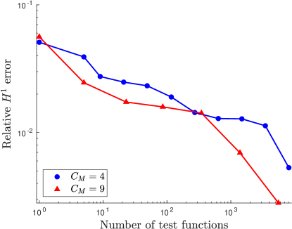
Figure 3: Strategy #1: Relative $H^{1}$ errors obtained at the end of each training iteration for $C_{M}=4$ (blue circles) and $C_{M}=9$ (red triangles).

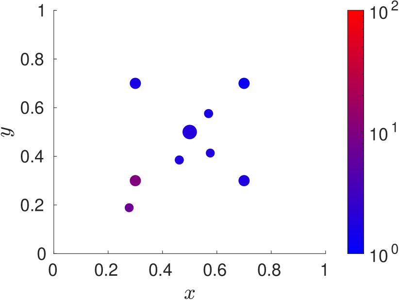
4.a Representation of ${\cal P}_{2}$.

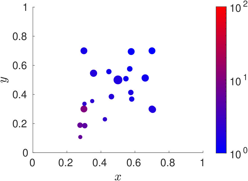
4.b Representation of ${\cal P}_{3}$.

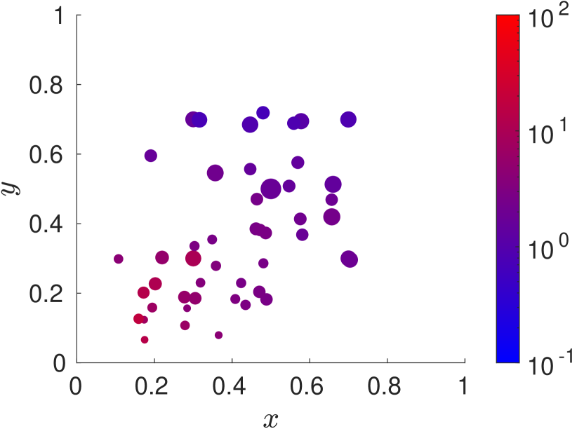
4.c Representation of ${\cal P}_{4}$.

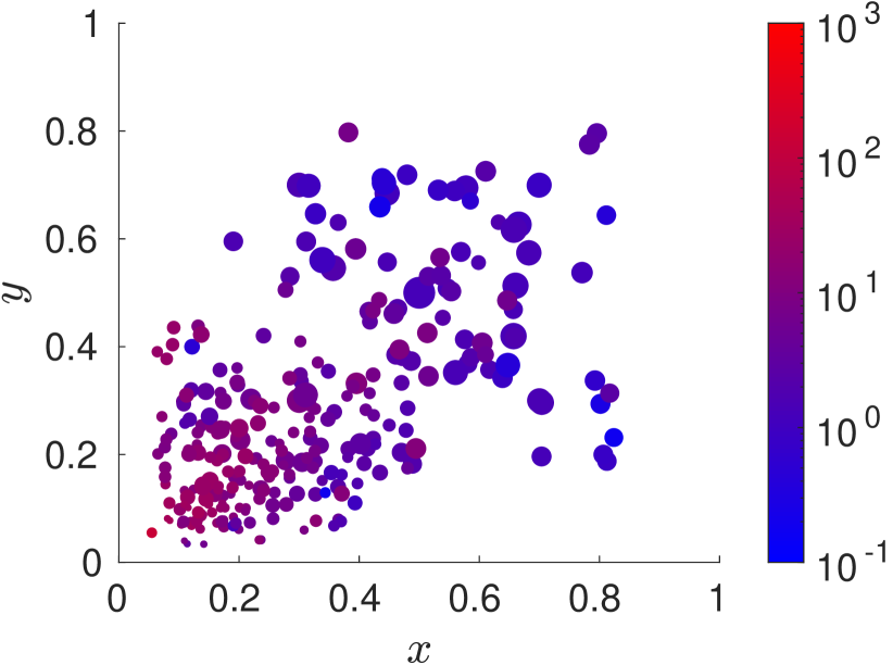
4.d Representation of ${\cal P}_{6}$.

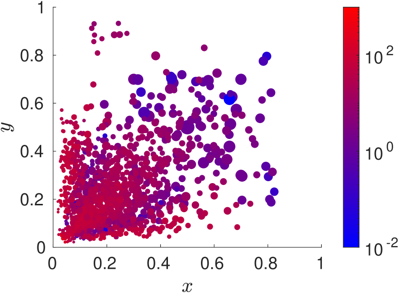
4.e Representation of ${\cal P}_{8}$.

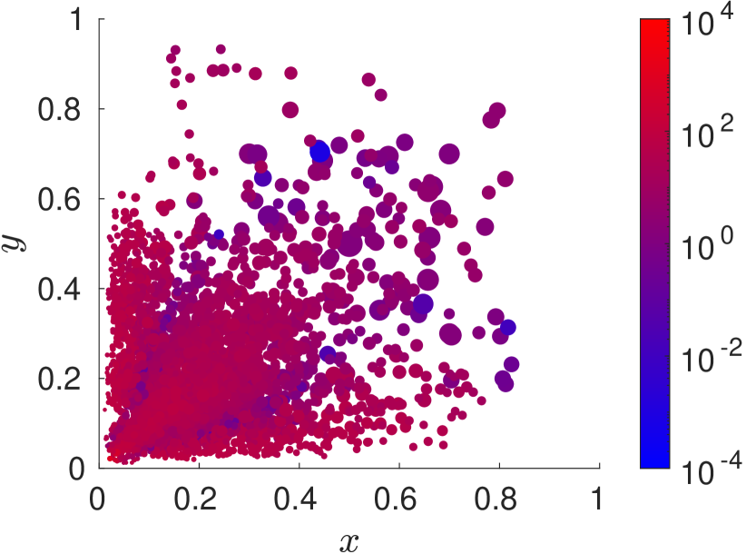
4.f Representation of ${\cal P}_{9}$.

Figure 4: Strategy #1: Patches used to train the MF-VPINN with $C_{M}=4$. Each dot represents a patch $P_{i}$, its position is the center $\bm{c_{P_{i}}}$ of the patch, its size is proportional to the patch size $h_{i}^{2}$, its color is associated with the quantity $\eta_{i}^{\gamma}$.

5.a Representation of ${\cal P}_{1}$.

5.b Representation of ${\cal P}_{2}$.

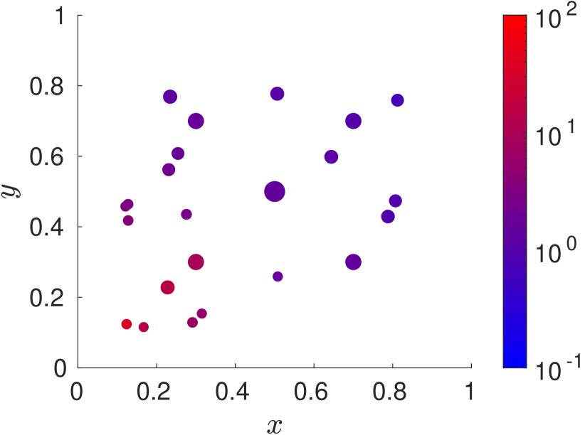
5.c Representation of ${\cal P}_{3}$.

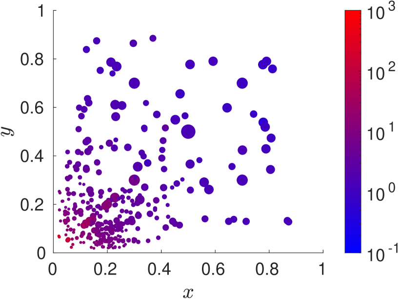
5.d Representation of ${\cal P}_{4}$.

5.e Representation of ${\cal P}_{5}$.

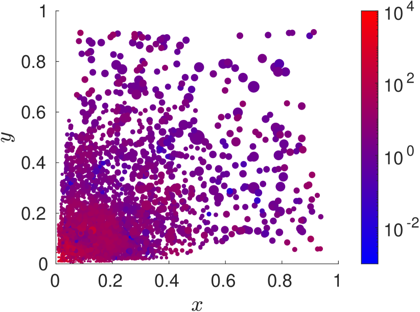
5.f Representation of ${\cal P}_{6}$.

Figure 5: Strategy #1: Patches used to train the MF-VPINN with $C_{M}=9$. Each dot represents a patch $P_{i}$, its position is the center $\bm{c_{P_{i}}}$ of the patch, its size is proportional to the patch size $h_{i}^{2}$, its color is associated with the quantity $\eta_{i}^{\gamma}$.

Strategy #2: Fixed patch centers

From the results discussed in Strategy #1, it can be observed that choosing the position of the new centers randomly may lead to non-uniform patches distribution in regions far from the singular point. In order to obtain better distributions, let us fix a priori the position of the new centers. Let us consider the reference patch $\hat{P}=(0,1)^{2}$ and the points:

$$\bm{\hat{c}_{1}}=(0.25,0.25),\hskip 28.45274pt\bm{\hat{c}_{2}}=(0.75,0.25),$$ (3.7)

$$\bm{\hat{c}_{3}}=(0.25,0.75),\hskip 28.45274pt\bm{\hat{c}_{4}}=(0.75,0.75),$$

when $C_{M}=4$ and

$$\bm{\hat{c}_{1}}=(0.2,0.2),\hskip 28.45274pt\bm{\hat{c}_{2}}=(0.2,0.5),\hskip 28.45274pt\bm{\hat{c}_{3}}=(0.2,0.8),$$ (3.8)

$$\bm{\hat{c}_{4}}=(0.5,0.2),\hskip 28.45274pt\bm{\hat{c}_{5}}=(0.5,0.5),\hskip 28.45274pt\bm{\hat{c}_{6}}=(0.5,0.8),$$

$$\bm{\hat{c}_{7}}=(0.8,0.2),\hskip 28.45274pt\bm{\hat{c}_{8}}=(0.8,0.5),\hskip 28.45274pt\bm{\hat{c}_{9}}=(0.8,0.8),$$

when $C_{M}=9$. At the end of the $(m-1)$-th training iteration, if $\eta_{i}^{\gamma}\in\overline{\bm{\eta}}_{m-1}$, the $C_{M}$ centers inside $P_{i}$ are chosen as $\bm{c_{P_{i}^{k}}}=M_{i}(\bm{\hat{c}_{k}})$, $k=1,\dots,C_{M}$. Once more, to avoid patches partially outside $\Omega$, we update such centers as in (3.6). We highlight that, defining the new centers as in (3.7) and in (3.8) and the length $h_{i}^{k}$ of the edges of the new patches as in Strategy #1, then the new patches with centres inside $P_{i}$ form a cover of $P_{i}$, i.e. $P_{i}\subsetneq\cup_{k=1}^{C_{M}}P_{i}^{k}$. Such a property does not hold if the new centers are randomly chosen.

Training a MF-VPINN with such a strategy leads to more accurate results. The error decays are shown in Fig. 6, whereas a comparison with the previous one will be presented in Section 3.3. The patch distributions, for $C_{M}=4$ and $C_{M}=9$, are shown in Fig. 7 and 8 respectively. Analyzing such distributions, it can be noted that the patches still accumulate near the origin as expected. However, it is possible to observe that there are regions that are only covered by the largest patches. This phenomenon is more evident when $C_{M}=4$. To avoid such a phenomenon, we aim at inserting more patches far from the origin in order to train the MF-VPINN in the entire domain with a more balanced set of patches.

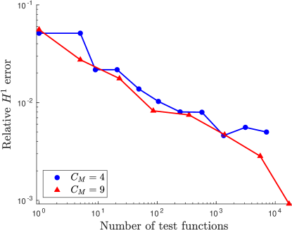
Figure 6: Strategy #2: Relative $H^{1}$ errors obtained at the end of each training iteration for $C_{M}=4$ (blue circles) and $C_{M}=9$ (red triangles).

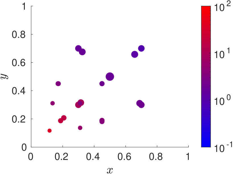
7.a Representation of ${\cal P}_{3}$.

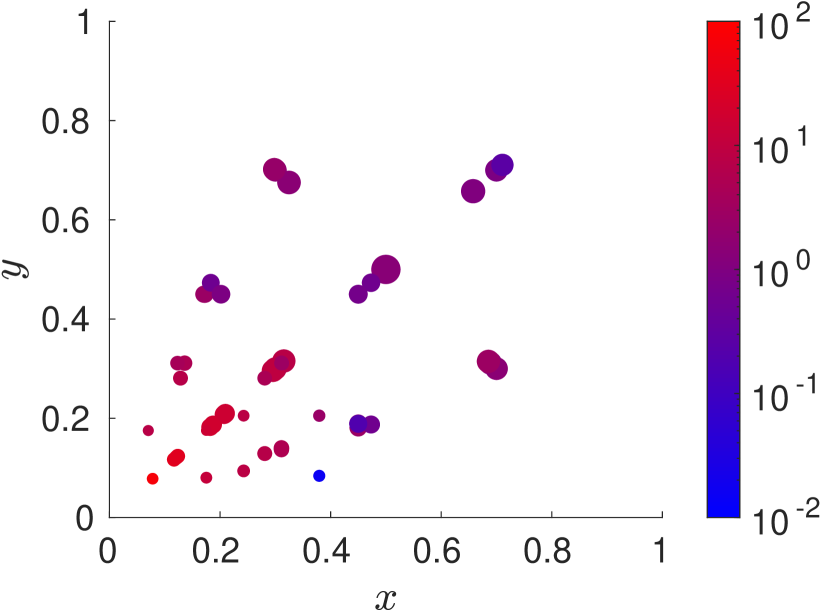
7.b Representation of ${\cal P}_{4}$.

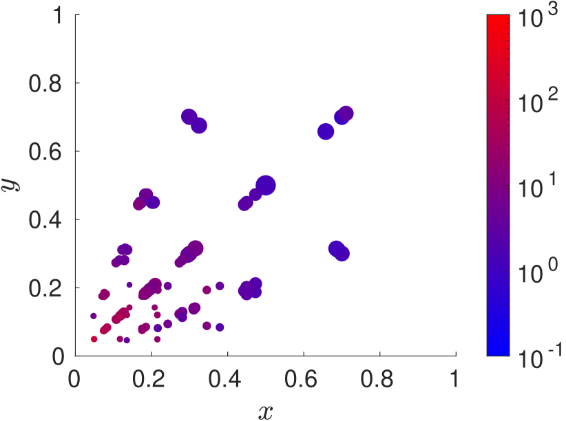
7.c Representation of ${\cal P}_{5}$.

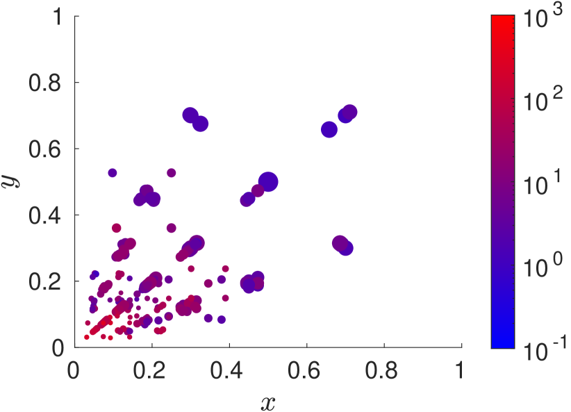
7.d Representation of ${\cal P}_{6}$.

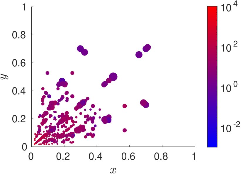
7.e Representation of ${\cal P}_{7}$.

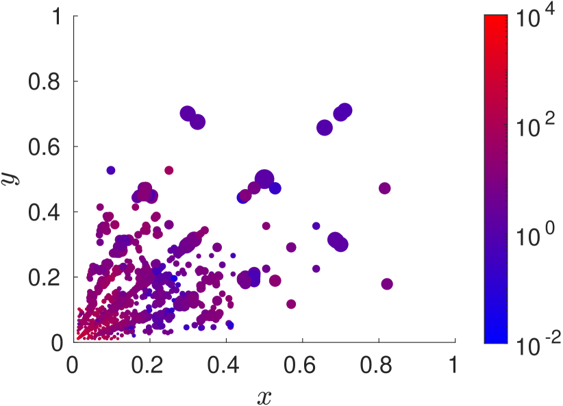
7.f Representation of ${\cal P}_{8}$.

Figure 7: Strategy #2: Patches used to train the MF-VPINN with $C_{M}=4$. Each dot represents a patch $P_{i}$, its position is the center $\bm{c_{P_{i}}}$ of the patch, its size is proportional to the patch size $h_{i}^{2}$, its color is associated with the quantity $\eta_{i}^{\gamma}$.

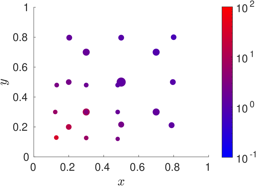
8.a Representation of ${\cal P}_{2}$.

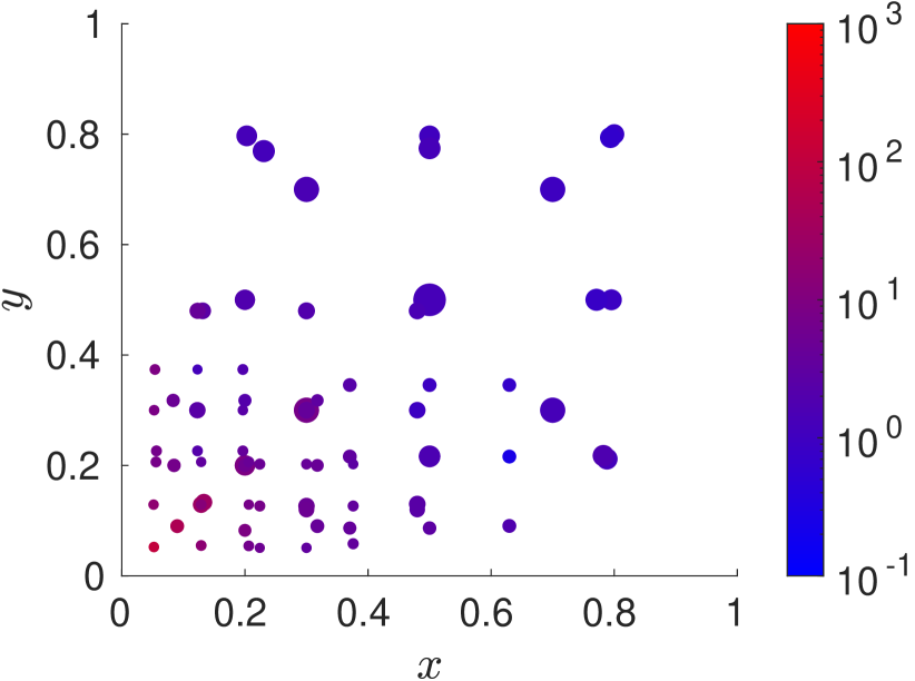
8.b Representation of ${\cal P}_{3}$.

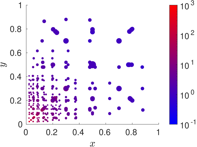
8.c Representation of ${\cal P}_{4}$.

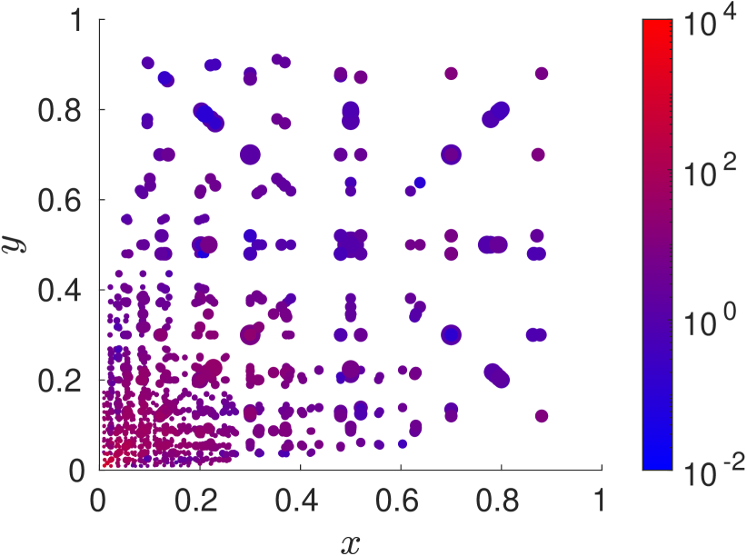
8.d Representation of ${\cal P}_{5}$.

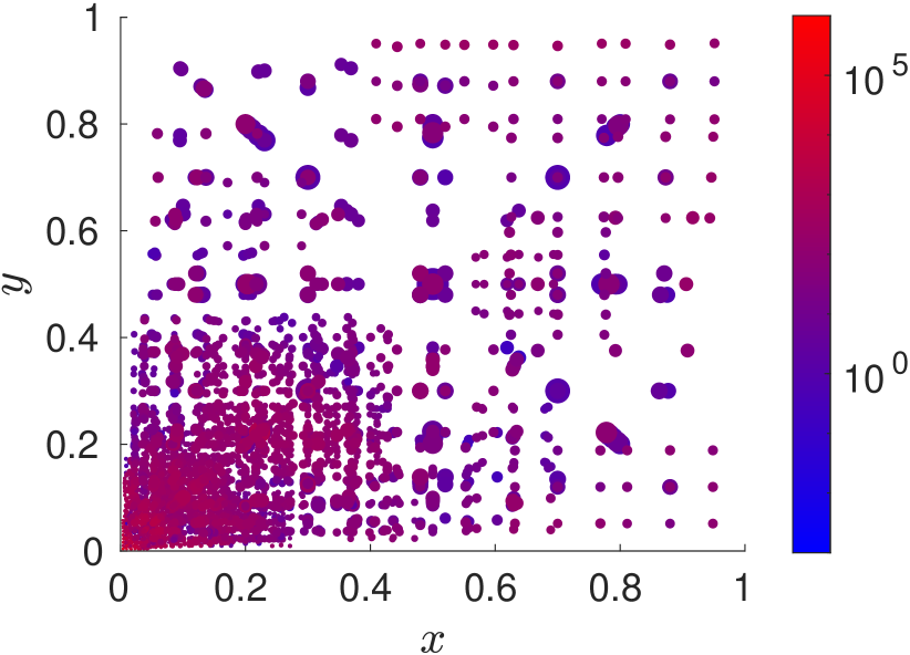
8.e Representation of ${\cal P}_{6}$.

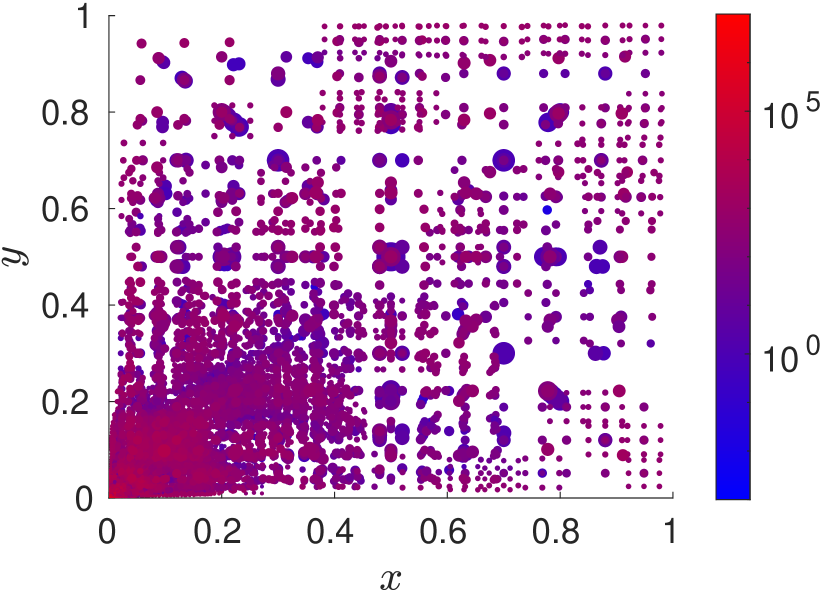
8.f Representation of ${\cal P}_{7}$.

Figure 8: Strategy #2: Patches used to train the MF-VPINN with $C_{M}=9$. Each dot represents a patch $P_{i}$, its position is the center $\bm{c_{P_{i}}}$ of the patch, its size is proportional to the patch size $h_{i}^{2}$, its color is associated with the quantity $\eta_{i}^{\gamma}$.

Strategy #3: Fixed patch centers and small level gap strategy

In order to ensure better patches distributions, let us consider a new criterion to choose the position and the size of the new patches. We name this strategy small level gap strategy because it penalizes patches distributions with large differences between the levels of the smallest patches and the ones of the largest patches.

We denote by $k$-th level patch any patch $P_{i}$ such that $P_{i}\in{\cal P}_{k}$ and $P_{i}\notin{\cal P}_{k^{\prime}}$ for any $k^{\prime}<k$. With this notation, it is possible to group all the patches according to their level. To do so, we denote by $L_{\ell}$ the set of $k$-th level patches with $k\leq\ell$. Let us consider the $m$-th training iteration. We define ${\bm{\eta}}_{\text{sort}}^{\ell}$ as the array containing the elements $\eta_{i}^{\gamma}$ of ${\bm{\eta}}_{\text{sort}}$ (maintaining the same ordering) such that $P_{i}\in L_{\ell}$. We also denote by $\overline{\bm{\eta}}_{m,\ell}$ the array containing the first $\tau_{m}^{\ell}=\min\{\tau_{m},\text{dim}(L_{\ell})\}$ elements of ${\bm{\eta}}_{\text{sort}}^{\ell}$. Note that $\overline{\bm{\eta}}_{m,\ell}$ is the equivalent of $\overline{\bm{\eta}}_{m}$ for patches in $L_{\ell}$.

In order to generate the new patches in ${\cal P}_{m+1}\backslash{\cal P}_{m}$, let us add $C_{M}$ new patches in any patch $P_{i}$ such that $\eta_{i}^{\gamma}\in\overline{\bm{\eta}}_{m}\cup\overline{\bm{\eta}}_{m,\ell}$. The centers and sizes of the new patches are chosen as in Strategy #2. This allows us to exploit the fact that $P_{i}\subsetneq\cup_{k=1}^{C_{M}}P_{i}^{k}$ to remove the patches $P_{i}$ such that $\eta_{i}^{\gamma}\in\overline{\bm{\eta}}_{m}\cup\overline{\bm{\eta}}_{m,\ell}$ from the new set of patches ${\cal P}_{m+1}$. We remark that such patches cannot be removed when the centers are randomly chosen as in Strategy #1 because, in that case, ${\cal P}_{m+1}$ would not be a cover of $\Omega$ anymore.

We also highlight that, removing the patches $P_{i}$ such that $\eta_{i}^{\gamma}\in\overline{\bm{\eta}}_{m}\cup\overline{\bm{\eta}}_{m,\ell}$ and choosing $A_{\text{ratio}}=1$, it is possible to satisfy the inequality:

$$\sum_{P_{i}\in{\cal P}_{m+1}}|P_{i}|\leq C|\Omega|,$$

for any $m\in{\mathbb{N}}$ and with $C>0$ independent of $m$. Such bound on the sum of the area of the patches is useful to ensure that there exists a number $N_{\text{patch\_per\_point}}$ such that any point inside $\Omega$ belongs to at most $N_{\text{patch\_per\_point}}$ patches. This property is useful to derive global error indicators. We choose to maintain $A_{\text{ratio}}=1.25$ to compare the numerical results with the ones obtained using the previous strategies and to consider overlapping patches.

We train a MF-VPINN with $C_{M}=4$ and $C_{M}=9$ as in the previous tests. The corresponding error decays are shown in Fig. 9. It can be observed that the error decreases in a smoother way and that, as in the previous tests, choosing $C_{M}=4$ or $C_{M}=9$ does not lead to significant differences in the error behaviour. The patches used during the training are represented in Fig. 10 and 11. We highlight that, when compared with the patches distributions in Strategy #2, there exist much more patches far from the origin and, most importantly, the closer the center of a patch to the origin, the smaller its size. Even though the error decays with $C_{M}=4$ and $C_{M}=9$ are qualitatively similar, it should be noted that the patches distribution with $C_{M}=9$ is more skewed. In fact its patches can be clustered in two subgroups: the first one containing larger patches and covering most of the domain, the second one containing only small patches with centers very close to the origin. A similar distribution is obtained with $C_{M}=4$, even though it is characterized by a smoother transition between large and small patches.

In both cases, it can be observed that there are no large patches very close to small ones. This is in contrast with the distributions obtained in Strategy #2 and leads to more stable solvers. Indeed, even though the test functions are not related to a global triangulation on the entire domain $\Omega$, the current loss function is very similar to the one used in a standard VPINN with a good quality mesh, i.e. a mesh in which neighbour elements are similar in size and shape. On the other hand, in Strategy #2 there exist large patches that are very close to small ones; this is equivalent to training a VPINN on a very poor quality mesh. Such meshes, in the context of FEM, are strictly related to convergence and accuracy issues.

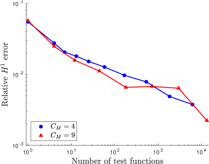
Figure 9: Strategy #3: Relative $H^{1}$ errors obtained at the end of each training iteration for $C_{M}=4$ (blue circles) and $C_{M}=9$ (red triangles).

10.a Representation of ${\cal P}_{3}$.

10.b Representation of ${\cal P}_{5}$.

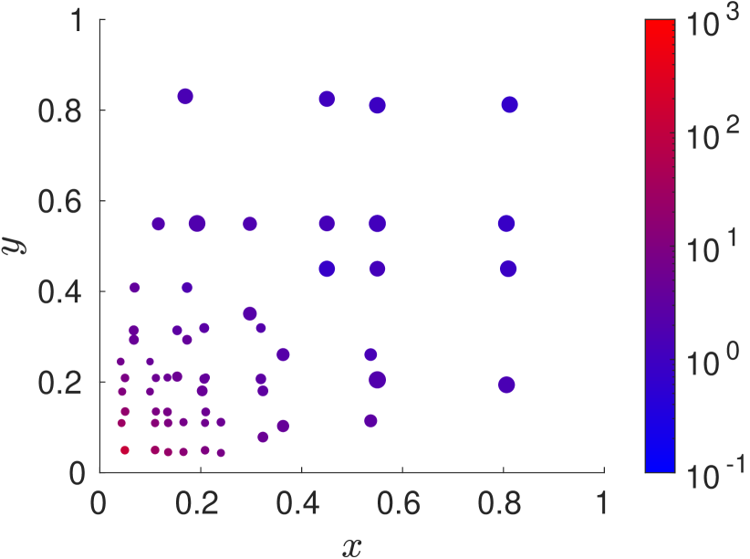
10.c Representation of ${\cal P}_{6}$.

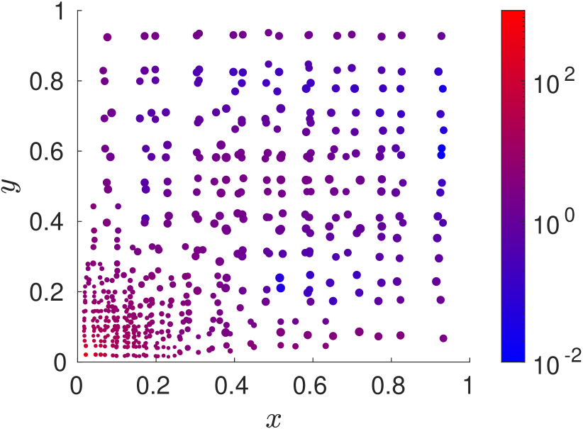
10.d Representation of ${\cal P}_{7}$.

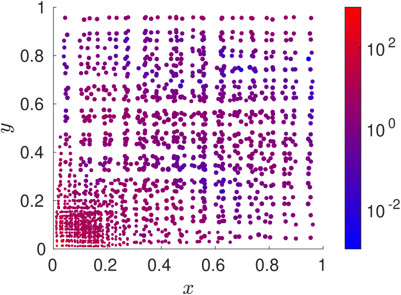
10.e Representation of ${\cal P}_{8}$.

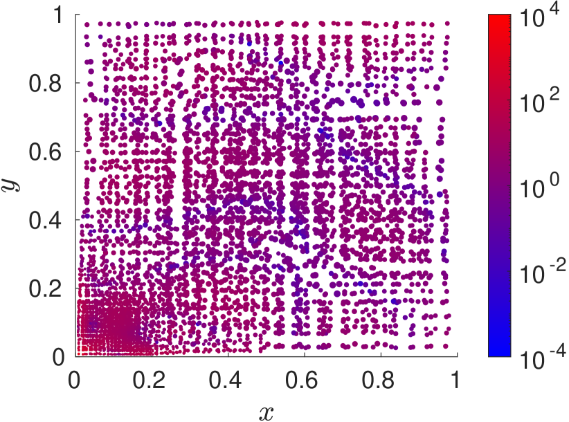
10.f Representation of ${\cal P}_{9}$.

Figure 10: Strategy #3: Patches used to train the MF-VPINN with $C_{M}=4$. Each dot represents a patch $P_{i}$, its position is the center $\bm{c_{P_{i}}}$ of the patch, its size is proportional to the patch size $h_{i}^{2}$, its color is associated with the quantity $\eta_{i}^{\gamma}$.

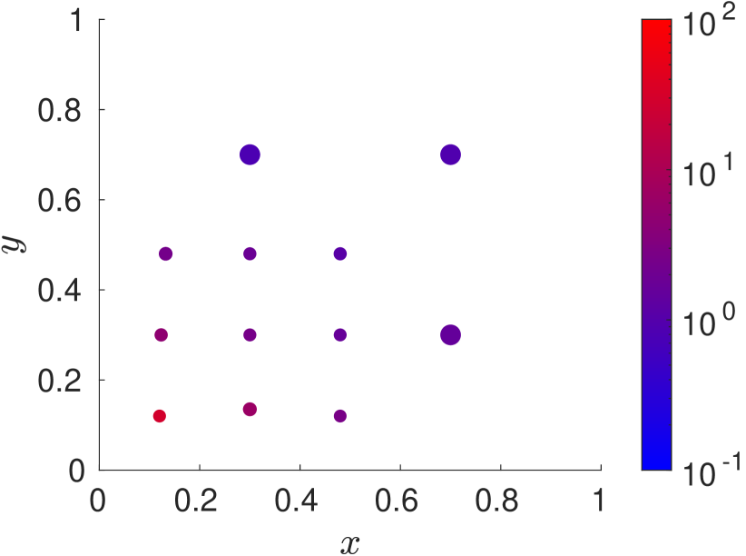
11.a Representation of ${\cal P}_{2}$.

11.b Representation of ${\cal P}_{3}$.

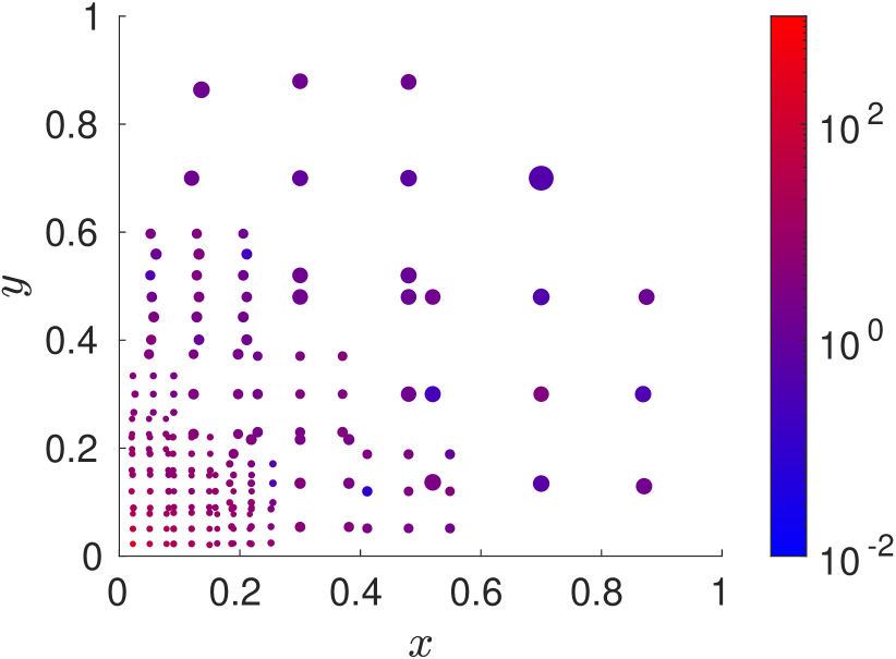
11.c Representation of ${\cal P}_{4}$.

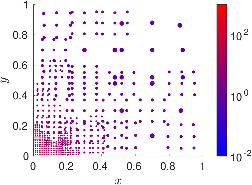
11.d Representation of ${\cal P}_{5}$.

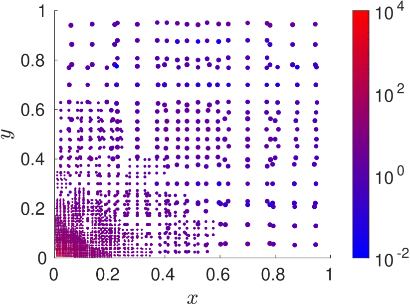
11.e Representation of ${\cal P}_{6}$.

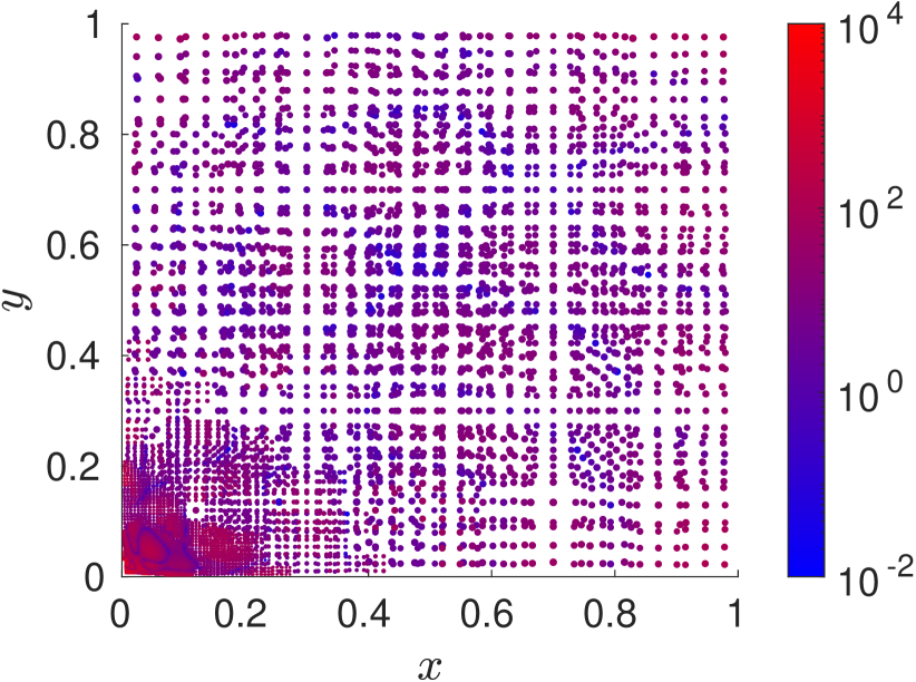
11.f Representation of ${\cal P}_{7}$.

Figure 11: Strategy #3: Patches used to train the MF-VPINN with $C_{M}=9$. Each dot represents a patch $P_{i}$, its position is the center $\bm{c_{P_{i}}}$ of the patch, its size is proportional to the patch size $h_{i}^{2}$, its color is associated with the quantity $\eta_{i}^{\gamma}$.

3.3 The importance of the error indicator

As discussed in the previous sections, we use the error indicator described in Section 2.3 to interrupt the training and to decide where the new patches has to be inserted to maximize the accuracy. In this section the advantages of such a choice are described.

Since each set ${\cal P}_{m}$ is a cover of $\Omega$, the quantity $ES_{m}=\sum_{i=1}^{\text{dim}({\cal P}_{m})}\eta_{i}$ is an indicator of the global $H^{1}$ error $\|u-u^{\mathcal{NN}}\|_{1}$ on the entire domain $\Omega$. Therefore, tracking its behaviour during the training is equivalent to track the one of the unknown $H^{1}$ error. Such information is used to implement an early stopping strategy to reduce the computational cost of the iterative training. At the beginning of the $m$-th training iteration, all the vectors and sparse matrices required to compute $ES_{m}$ are computed in a preprocessing phase. When such data structures are available, the error indicator can be assembled suitably combining basic algebraic operations.

We assemble $ES_{m}$ every $N_{\text{check}}$ epochs and store the best value obtained during the training, together with the corresponding neural network trainable parameters. Then, if no improvements is obtained in $p\cdot N_{\text{check}}$ epochs, the training is interrupted and the neural network parameters associated with the best value of $ES_{m}$ are restored. Here $p$ is a tunable parameter named patience. The first $N_{\text{negl}}^{m}$ epochs are neglected because they are often characterized by strong oscillations due to the optimizer initialization and the different loss function. In the numerical experiment we use $N_{\text{check}}=10$, $p=10$, $N_{\text{negl}}^{m}=100(m+1)$.

Two typical scenarios are shown in Fig. 12. In the top row the behaviours of $ES_{m}$ and of $c\|u-u^{\mathcal{NN}}\|_{1}$ are shown. Here $c$ is a scaling parameters, used for visualization purposes, chosen such that $ES_{m}$ and $c\|u-u^{\mathcal{NN}}\|_{1}$ coincide at the beginning of the training. Indeed, $\|u-u^{\mathcal{NN}}\|_{1}$ is about two orders of magnitude smaller than $ES_{m}$. Nevertheless, it can be noted that these two quantities display very similar behaviours during the training. In the bottom row, instead, we represent the corresponding loss function decay. The left column is associated with the training performed using the patches in ${\cal P}_{6}$ shown in Fig. 55.f, the right column with the one performed using the patches in ${\cal P}_{2}$ in Fig. 1111.a. We remark that the loss function, $ES_{m}$ and $c\|u-u^{\mathcal{NN}}\|$ are evaluated in the same epochs and that, in real applications, it is not possible to explicitly compute $c\|u-u^{\mathcal{NN}}\|$ since $u$ is not known. Moreover, since we use the L-BFGS optimizer, the neural network is evaluated multiple times on the entire training set in each epoch. Therefore, on the $x$-axis of Fig. 12 we show the number of neural network evaluations instead of the number of epochs.

It can be noted that the behaviour of the quantities shown in the left column is qualitatively different from the ones in the right column. In fact, when the MF-VPINN is trained with ${\cal P}_{6}$ of Fig. 55.f, the error, the error indicator and the loss function decrease in similar ways. Therefore, there is no need to interrupt the training early since the accuracy is improving minimizing the loss function. On the other hand, when the MF-VPINN is trained with ${\cal P}_{2}$ of Fig. 1111.a, the loss decreases even when the error and the error indicator increase or remain constant. In this case it is convenient to interrupt the training, since minimizing the loss function further would lead to more severe overfitting phenomena and a loss in accuracy and efficiency. At the end of the training, the neural network trainable parameters corresponding to the best value of $ES_{2}$ are restored. We highlight that such a phenomenon, observed in [4] too, highlights the fact that the minimization of the loss function generates spurious oscillations that cannot be controlled and ruin the model accuracy. The issue can be partially alleviated with the adopted regularization or completely removed using inf-sup stable models as in [5].

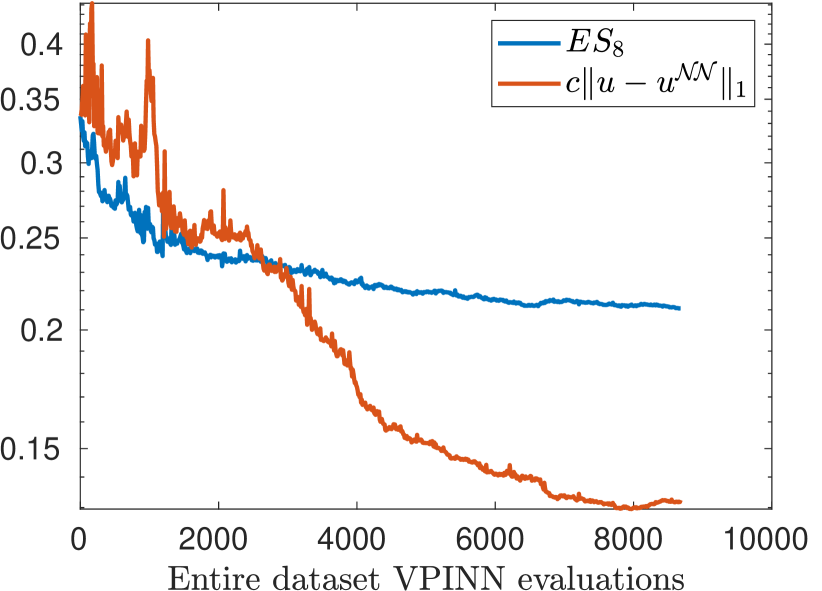
12.a $ES_{4}$ and $c\|u-u^{\mathcal{NN}}\|$ for patches in Fig. 44.c.

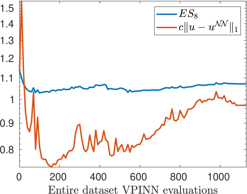
12.b $ES_{2}$ and $c\|u-u^{\mathcal{NN}}\|$ for patches in Fig. 1111.a.

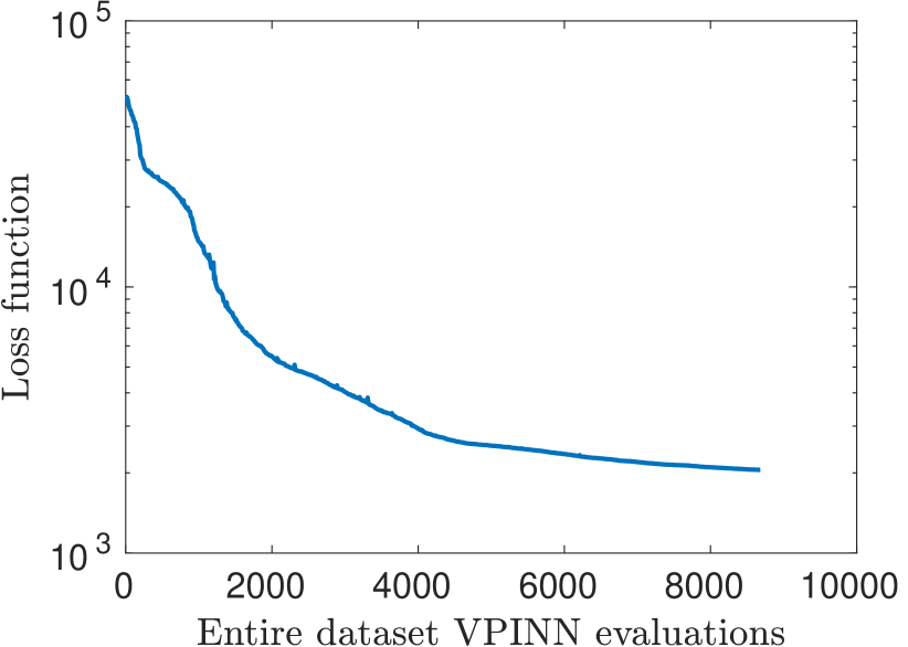
12.c Loss function for patches in Fig. 44.c.

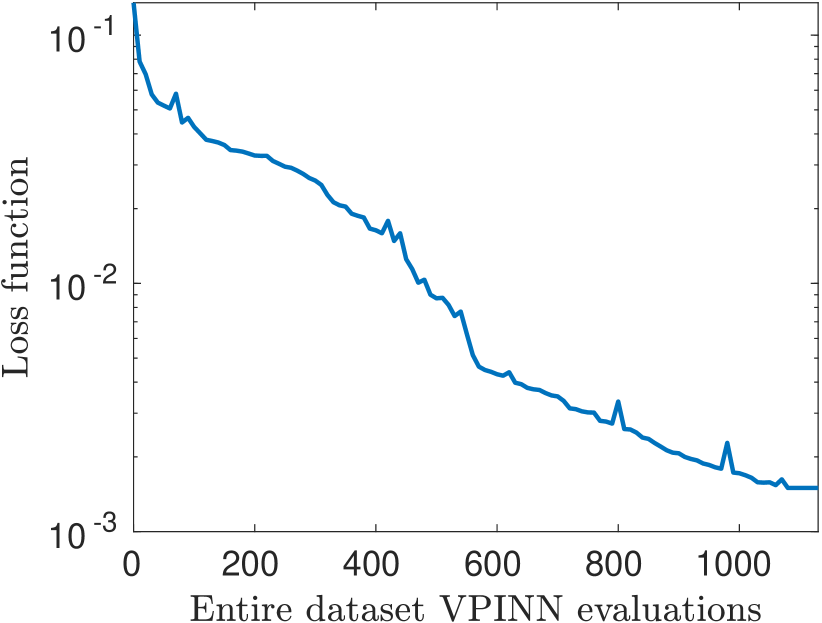
12.d Loss function for patches in Fig. 1111.a.

Figure 12: Top row: error indicator $ES_{m}$ and rescaled $H^{1}$ error $c\|u-u^{\mathcal{NN}}\|$. Bottom row: loss function. Left column: curves for the training with patches in ${\cal P}_{6}$ shown in Fig. 55.f. Right column: curves for the training with patches in ${\cal P}_{2}$ in Fig. 1111.a.

Let us now analyze the consequences of choosing the position of the new patches without using the error indicator. To do so, we consider Strategy #1 with $C_{M}=4$ but, instead of considering the new centers inside the patches $P_{i}$ with the highest values of $\eta_{i}^{\gamma}$, we add them inside the patches with the highest values of $r_{h,i}^{2}(u^{\mathcal{NN}})$. Using the equation residuals is a common choice in PINN adaptivity because the residuals describe how accurately the neural network satisfies the PDE in that point. The obtained error decay is shown in Fig. 1313.a, where we denote this strategy by Strategy #4. It can be seen that the accuracy is worse than the ones obtained with the other strategies and that the convergence rate with respect to the number of patches is lower. In such a figure we also compare the MF-VPINN with a standard VPINN trained with test functions defined on Delaunay meshes. Note that, when Strategy #2 or Strategy #3 are adopted, the MF-VPINN is more accurate than a simple VPINN, even though its main advantage resides in being a mesh-free method.

The convergence rates are shown in table 1. We highlight that, due to the low regularity of the solution, the expected convergence rate with respect to the number of test functions of a FEM solution computed on uniform refinements is -1/3. Note that the convergence rate of the proposed MF-VPINN method is still close to -1/3, even though it is a meshfree method. For completeness, we also remark that, if an adaptive FEM is used, the rate of convergence depends on the FEM order.

$C_{M}$	Strategy #1	Strategy #2	Strategy #3	Strategy #4	Reference VPINN
4	-0.213	-0.295	-0.283	-0.105	-0.232
9	-0.294	-0.376	-0.287	-0.182	-0.232

Table 1: Convergence rates with respect to the number of test functions obtained with the different strategies.

Coherently with Fig. 13, the best strategies are Strategy #2 and Strategy #3, whereas the worst one is Strategy #4, which does not exploit the error indicator. The poor performance of Strategy #4 can also be explained analyzing the corresponding patches distribution. Such distribution is shown in Fig. 14 and highlights that the patches do not accumulate near the origin because the residuals of the patches closer to it are not significantly higher than the other ones. In particular, note the different colors in Fig. 4 and 14, since in both cases we randomly choose the position of $C_{M}=4$ centers inside the selected patches. Such a property is explained by the fact that, in order to minimize the loss function, the optimizer does not focus on specific regions of the domain. Therefore, the orders of magnitude of all the residuals with similar size are very close to each other regardless of the position of the corresponding patches. As discussed commenting Fig. 12, we can conclude that the value of the residuals is not a good indicator of the actual error.

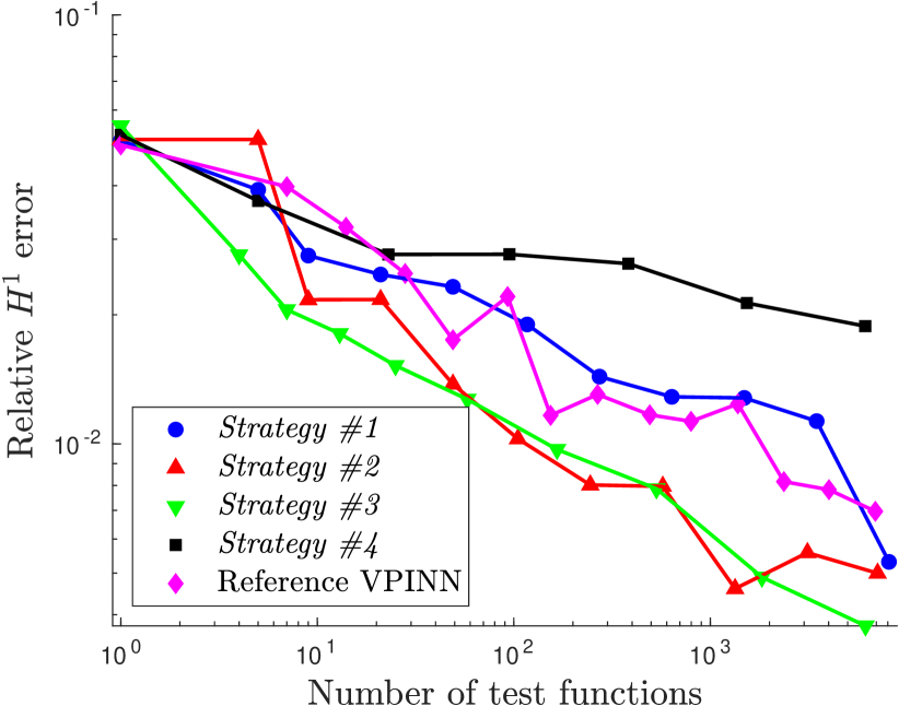
13.a $C_{M}=4$.

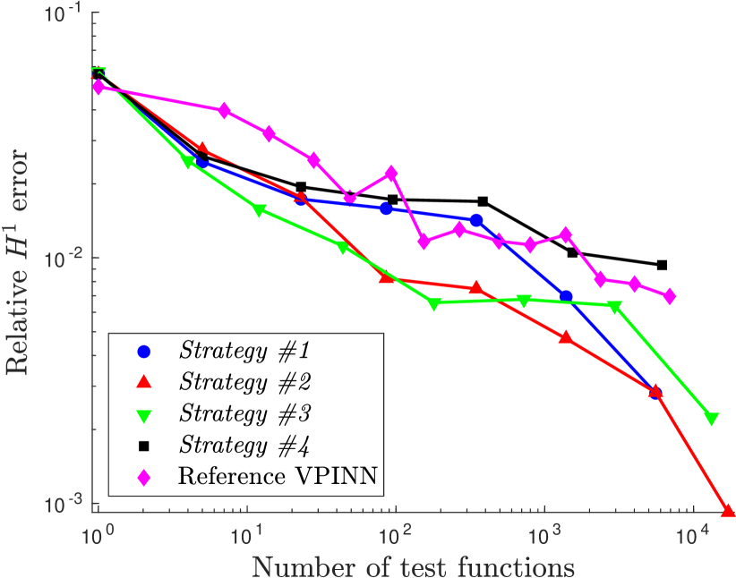
13.b $C_{M}=9$.

Figure 13: Comparison between the relative $H^{1}$ errors obtained at the end of each training iteration with different strategies to choose the position of the new patches.

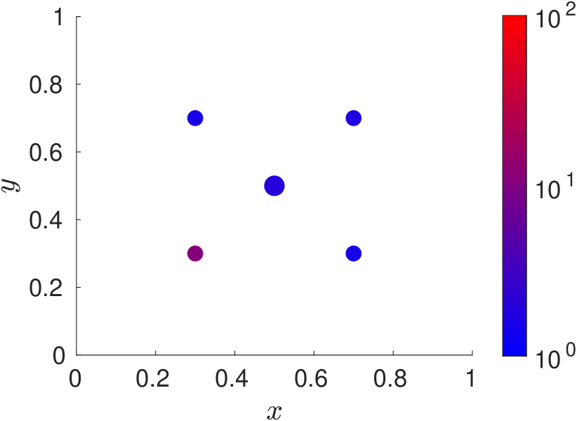
14.a Representation of ${\cal P}_{1}$.

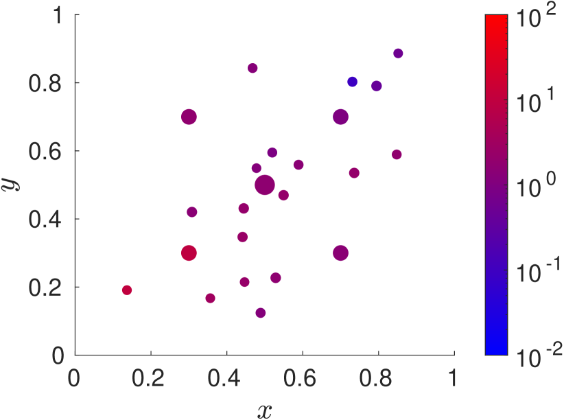
14.b Representation of ${\cal P}_{2}$.

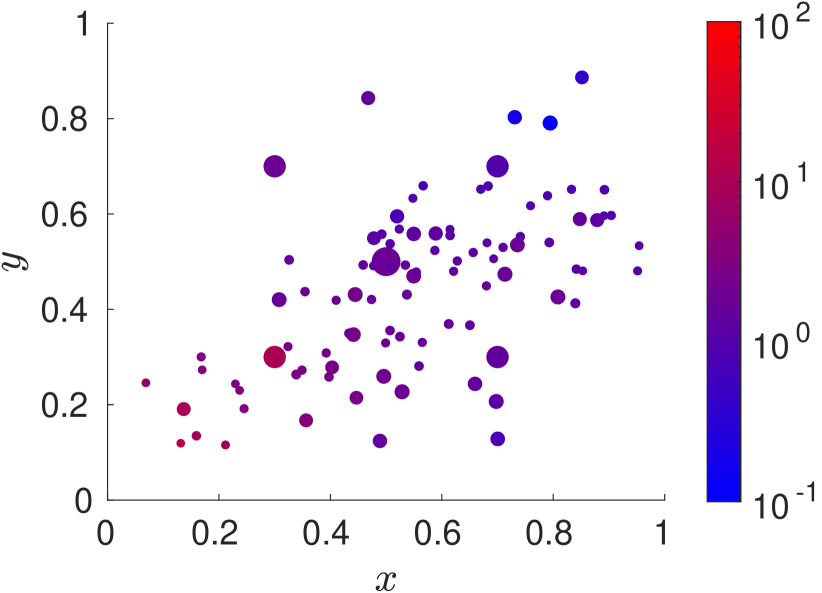
14.c Representation of ${\cal P}_{3}$.

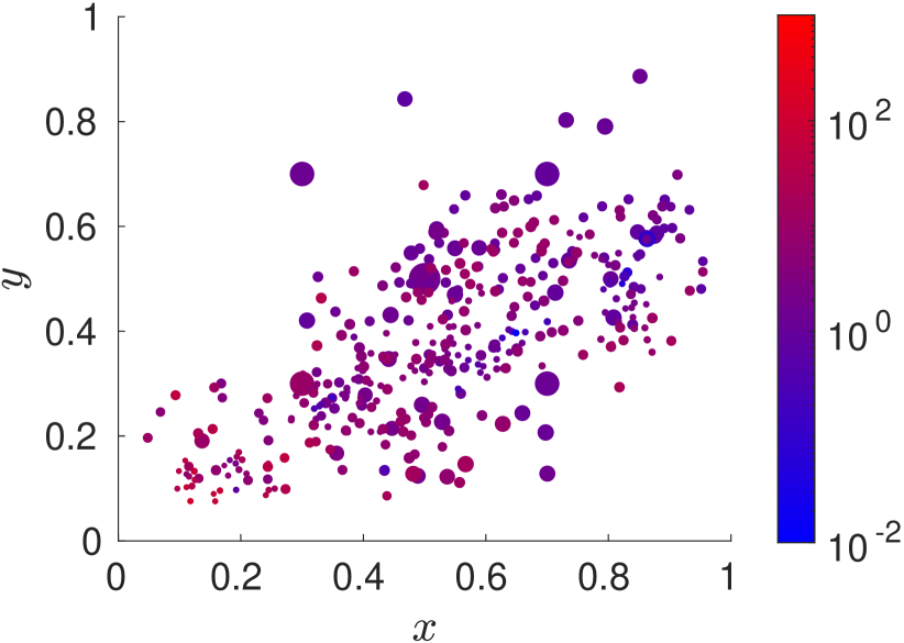
14.d Representation of ${\cal P}_{4}$.

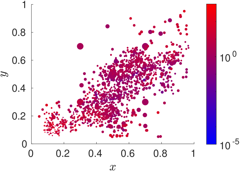
14.e Representation of ${\cal P}_{5}$.

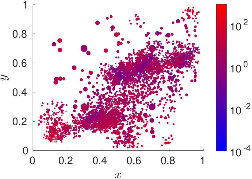
14.f Representation of ${\cal P}_{6}$.

Figure 14: Strategy #4: Patches used to train the MF-VPINN with $C_{M}=4$. Each dot represents a patch $P_{i}$, its position is the center $\bm{c_{P_{i}}}$ of the patch, its size is proportional to the patch size $h_{i}^{2}$, its color is associated with the quantity $r_{h,i}^{2}(u^{\mathcal{NN}})$.

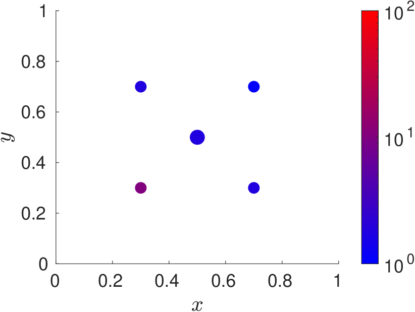
15.a Representation of ${\cal P}_{1}$.

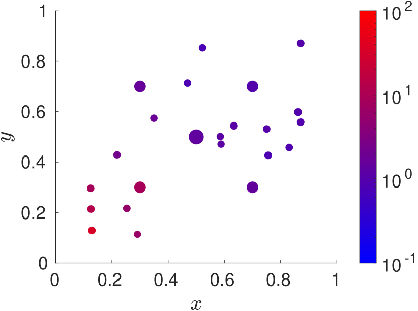
15.b Representation of ${\cal P}_{2}$.

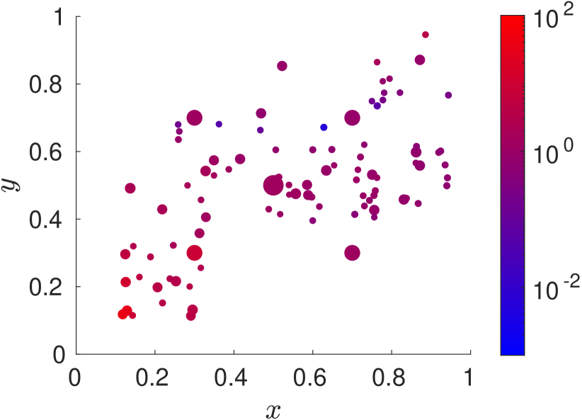
15.c Representation of ${\cal P}_{3}$.

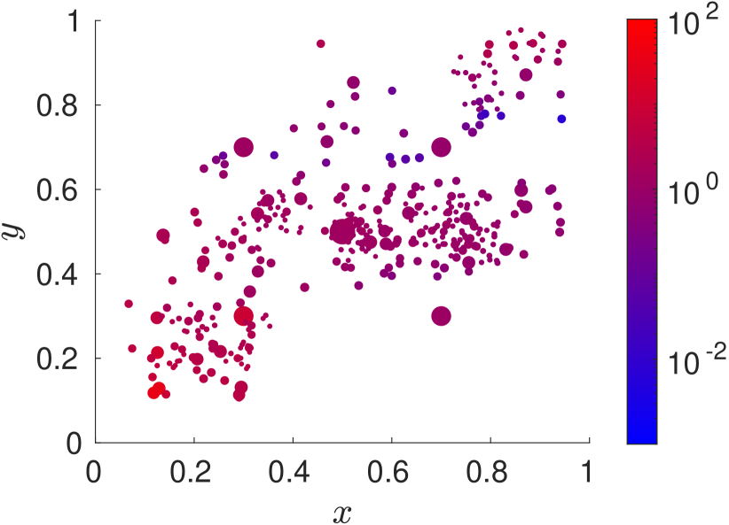
15.d Representation of ${\cal P}_{4}$.

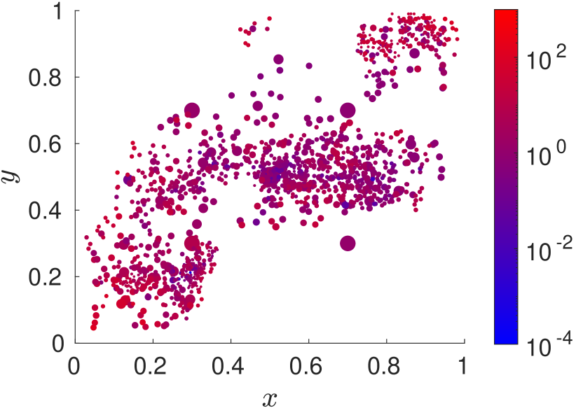
15.e Representation of ${\cal P}_{5}$.

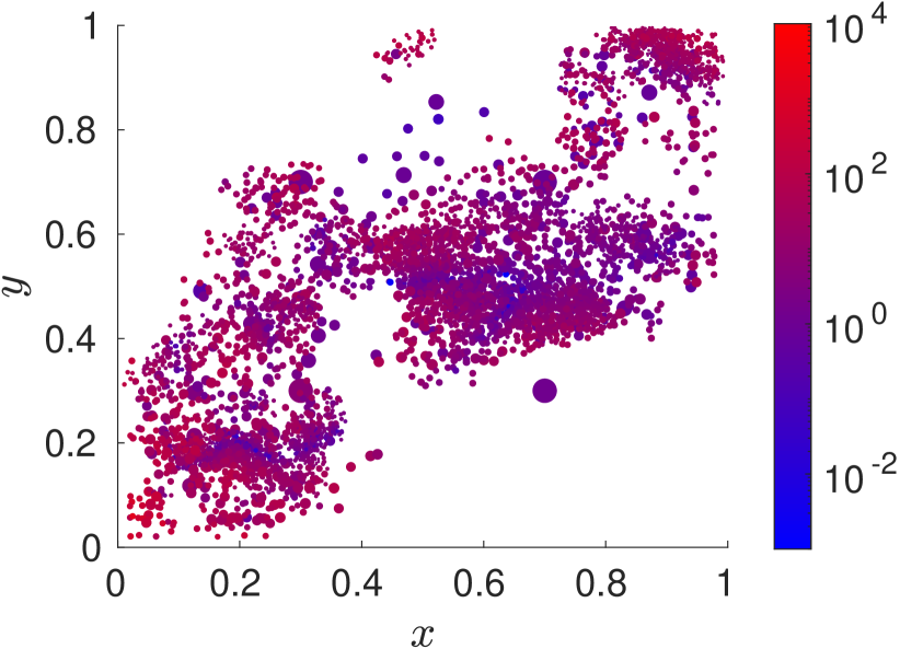
15.f Representation of ${\cal P}_{6}$.

Figure 15: Strategy #4: Patches used to train the MF-VPINN with $C_{M}=9$. Each dot represents a patch $P_{i}$, its position is the center $\bm{c_{P_{i}}}$ of the patch, its size is proportional to the patch size $h_{i}^{2}$, its color is associated with the quantity $r_{h,i}^{2}(u^{\mathcal{NN}})$.

4 Conclusion

In this work we presented a Meshfree Variational Physics Informed Neural Network (MF-VPINN). It is a PINN trained using the PDE variational formulation that does not require the generation of a global triangulation of the entire domain. In order to generate the test functions involved in the loss computation, we use an a posteriori error estimator based on the one discussed in [4]. Using such error estimator it is possible to add test functions only in regions in which the error is higher, thus increasing the efficiency of the method.

We discuss several strategies to generate the set of test functions. We observe that adding few test functions inside the patches associated with higher errors while ensuring a smooth transition between regions with large patches and regions with small patches is the best way to obtain accurate solutions. We also show that, if the a posteriori error indicator is not used, the model accuracy decreases and the training is slower.

In this paper we only focus on second-order elliptic problem even though VPINNs can be used to solve more complex problems. In a forthcoming paper, we will adapt the a posteriori error estimator and analyze the MF-VPINN performance on other PDEs. Moreover, we are interested in the analysis of the approach in more complex domains (in which the patches have to be suitably deformed) and in high-dimensional problems, where using a standard VPINN is not practical.

References

- [1] M. Abadi et al., TensorFlow: Large-scale machine learning on heterogeneous systems, 2015. Software available from tensorflow.org.
- [2] A. Baydin, B. Pearlmutter, A. Radul, and J. Siskind, Automatic differentiation in machine learning: a survey, Journal of machine learning research, 18 (2018).
- [3] C. Beck, M. Hutzenthaler, A. Jentzen, and B. Kuckuck, An overview on deep learning-based approximation methods for partial differential equations, Discrete and Continuous Dynamical Systems - B, (2022).
- [4] S. Berrone, C. Canuto, and M. Pintore, Solving PDEs by variational physics-informed neural networks: an a posteriori error analysis, Annali dell’Università di Ferrara, 68 (2022), pp. 575–595.
- [5] , Variational physics informed neural networks: the role of quadratures and test functions, Journal of Scientific Computing, 92 (2022), pp. 1–27.
- [6] S. Berrone, C. Canuto, M. Pintore, and N. Sukumar, Enforcing dirichlet boundary conditions in physics-informed neural networks and variational physics-informed neural networks, Heliyon, 9 (2023), p. e18820.
- [7] Z. Chen, Y. Liu, and H. Sun, Physics-informed learning of governing equations from scarce data, Nature Communications, 12 (2021).
- [8] S. Cuomo, V. S. Di Cola, F. Giampaolo, G. Rozza, M. Raissi, and F. Piccialli, Scientific machine learning through physics-informed neural networks: Where we are and what’s next, Journal of Scientific Computing, 92 (2022).
- [9] N. Demo, M. Strazzullo, and G. Rozza, An extended physics informed neural network for preliminary analysis of parametric optimal control problems, arXiv preprint arXiv:2110.13530, (2021).
- [10] H. Gao, L. Sun, and J. Wang, Phygeonet: physics-informed geometry-adaptive convolutional neural networks for solving parameterized steady-state pdes on irregular domain, Journal of Computational Physics, 428 (2021), p. 110079.
- [11] Q. Guo, Y. Zhao, C. Lu, and J. Luo, High-dimensional inverse modeling of hydraulic tomography by physics informed neural network (ht-pinn), Journal of Hydrology, 616 (2023), p. 128828.
- [12] A. Jagtap, E. Kharazmi, and G. Karniadakis, Conservative physics-informed neural networks on discrete domains for conservation laws: Applications to forward and inverse problems, Computer Methods in Applied Mechanics and Engineering, 365 (2020), p. 113028.
- [13] E. Kharazmi, Z. Zhang, and G. Karniadakis, VPINNs: Variational physics-informed neural networks for solving partial differential equations, arXiv preprint arXiv:1912.00873, (2019).
- [14] , -VPINNs: Variational physics-informed neural networks with domain decomposition, Computer Methods in Applied Mechanics and Engineering, 374 (2021), p. 113547.
- [15] D. Kingma and J. Ba, Adam: a method for stochastic optimization, arXiv preprint arXiv:1412.6980, (2014).
- [16] I. Lagaris, A. Likas, and D. Fotiadis, Artificial neural network methods in quantum mechanics, Computer Physics Communications, 104 (1997), pp. 1–14.
- [17] , Artificial neural networks for solving ordinary and partial differential equations, IEEE transactions on neural networks, 9 (1998), pp. 987–1000.
- [18] I. Lagaris, A. Likas, and D. Papageorgiou, Neural-network methods for boundary value problems with irregular boundaries, IEEE Transactions on Neural Networks, 11 (2000), pp. 1041–1049.
- [19] Z. Lawal, H. Yassin, D. Lai, and A. Che Idris, Physics-Informed Neural Network (PINN) Evolution and Beyond: A Systematic Literature Review and Bibliometric Analysis, Big Data and Cognitive Computing, 6 (2022).
- [20] A. Paszke et al., Pytorch: An imperative style, high-performance deep learning library, in Advances in Neural Information Processing Systems 32, Curran Associates, Inc., 2019, pp. 8024–8035.
- [21] L. Prechelt, Early stopping-but when?, in Neural Networks: Tricks of the trade, Springer, 1998, pp. 55–69.
- [22] J. Pu, J. Li, and Y. Chen, Solving localized wave solutions of the derivative nonlinear schrödinger equation using an improved pinn method, Nonlinear Dynamics, 105 (2021), pp. 1723–1739.
- [23] M. Raissi, P. Perdikaris, and G. Karniadakis, Physics informed deep learning (part i): Data-driven solutions of nonlinear partial differential equations, arXiv preprint arXiv:1711.10561, (2017).
- [24] , Physics informed deep learning (part ii): Data-driven solutions of nonlinear partial differential equations, arXiv preprint arXiv:1711.10566, (2017).
- [25] , Physics-informed neural networks: A deep learning framework for solving forward and inverse problems involving nonlinear partial differential equations, Journal of Computational Physics, 378 (2019), pp. 686–707.
- [26] J. Sirignano and K. Spiliopoulos, DGM: A deep learning algorithm for solving partial differential equations, Journal of Computational Physics, 375 (2018), pp. 1339–1364.
- [27] N. Sukumar and A. Srivastava, Exact imposition of boundary conditions with distance functions in physics-informed deep neural networks, Computer Methods in Applied Mechanics and Engineering, 389 (2022), p. 114333.
- [28] A. Tartakovsky, C. Marrero, P. Perdikaris, G. Tartakovsky, and D. Barajas-Solano, Learning parameters and constitutive relationships with physics informed deep neural networks, arXiv preprint arXiv:1808.03398, (2018).
- [29] F. Viana, R. Nascimento, A. Dourado, and Y. Yucesan, Estimating model inadequacy in ordinary differential equations with physics-informed neural networks, Computers & Structures, 245 (2021), p. 106458.
- [30] E. Weinan and B. Yu, The Deep Ritz method: a deep learning-based numerical algorithm for solving variational problems, Communications in Mathematics and Statistics, 6 (2018), pp. 1–12.
- [31] S. Wright, J. Nocedal, et al., Numerical Optimization, vol. 35, Springer, 1999.
- [32] L. Yang, X. Meng, and G. Karniadakis, B-PINNs: Bayesian physics-informed neural networks for forward and inverse PDE problems with noisy data, Journal of Computational Physics, 425 (2021), p. 109913.
- [33] L. Yang, D. Zhang, and G. Karniadakis, Physics-informed generative adversarial networks for stochastic differential equations, SIAM Journal on Scientific Computing, 42 (2020), pp. A292–A317.
- [34] L. Yuan, Y. Ni, X. Deng, and S. Hao, A-pinn: Auxiliary physics informed neural networks for forward and inverse problems of nonlinear integro-differential equations, Journal of Computational Physics, 462 (2022), p. 111260.
- [35] Y. Yucesan and F. Viana, Hybrid physics-informed neural networks for main bearing fatigue prognosis with visual grease inspection, Computers in Industry, 125 (2021), p. 103386.
- [36] C. Yuyao, L. Lu, G. Karniadakis, and L. Dal Negro, Physics-informed neural networks for inverse problems in nano-optics and metamaterials, Opt. Express, 28 (2020), pp. 11618–11633.
- [37] Y. Zhu, N. Zabaras, P. Koutsourelakis, and P. Perdikaris, Physics-constrained deep learning for high-dimensional surrogate modeling and uncertainty quantification without labeled data, Journal of Computational Physics, 394 (2019), pp. 56–81.