Towards Stable and Storage-efficient Dataset Distillation: Matching Convexified Trajectory

Abstract

The rapid evolution of deep learning and large language models has led to an exponential growth in the demand for training data, prompting the development of Dataset Distillation methods to address the challenges of managing large datasets. Among these, Matching Training Trajectories (MTT) has been a prominent approach, which replicates the training trajectory of an expert network on real data with a synthetic dataset. However, our investigation found that this method suffers from three significant limitations: 1. Instability of expert trajectory generated by Stochastic Gradient Descent (SGD); 2. Low convergence speed of the distillation process; 3. High storage consumption of the expert trajectory. To address these issues, we offer a new perspective on understanding the essence of Dataset Distillation and MTT through a simple transformation of the objective function, and introduce a novel method called Matching Convexified Trajectory (MCT), which aims to provide better guidance for the student trajectory. MCT leverages insights from the linearized dynamics of Neural Tangent Kernel methods to create a convex combination of expert trajectories, guiding the student network to converge rapidly and stably. This trajectory is not only easier to store, but also enables a continuous sampling strategy during distillation, ensuring thorough learning and fitting of the entire expert trajectory. Comprehensive experiments across three public datasets validate the superiority of MCT over traditional MTT methods.

1 Introduction

The advancement of deep learning has catalyzed an exponential surge in the requisite volume of training data (Wang et al., 2022). With the emergence of Large Language Models (LLMs), there has been a corresponding rise in model complexity, further intensifying the demand for extensive datasets to facilitate the training of these intricate models. However, collecting and managing large datasets presents significant challenges, including storage requirements, computational load, privacy concerns, and the costs of data labeling. To mitigate these challenges, Dataset Distillation (DD) has emerged as a compelling strategy (Wang et al., 2018). DD endeavors to distill the essence of a large, real-world dataset into a more compact, synthetic dataset that can train models with comparable efficacy.

In the landscape of DD methods, Matching Training Trajectories has emerged as a prominent approach. The MTT method aims to generate a synthetic dataset that guidea the learning trajectory of the student network to approximate the expert trajectory of this network on real data. However, upon closer examination, we identify several limitations inherent in traditional MTT approaches:

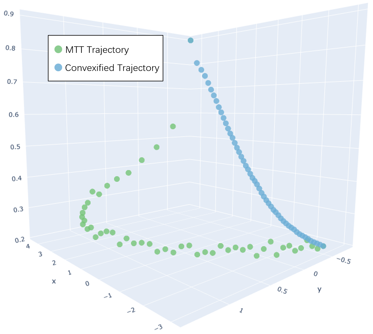
(a) Visualization of the expert trajectory.

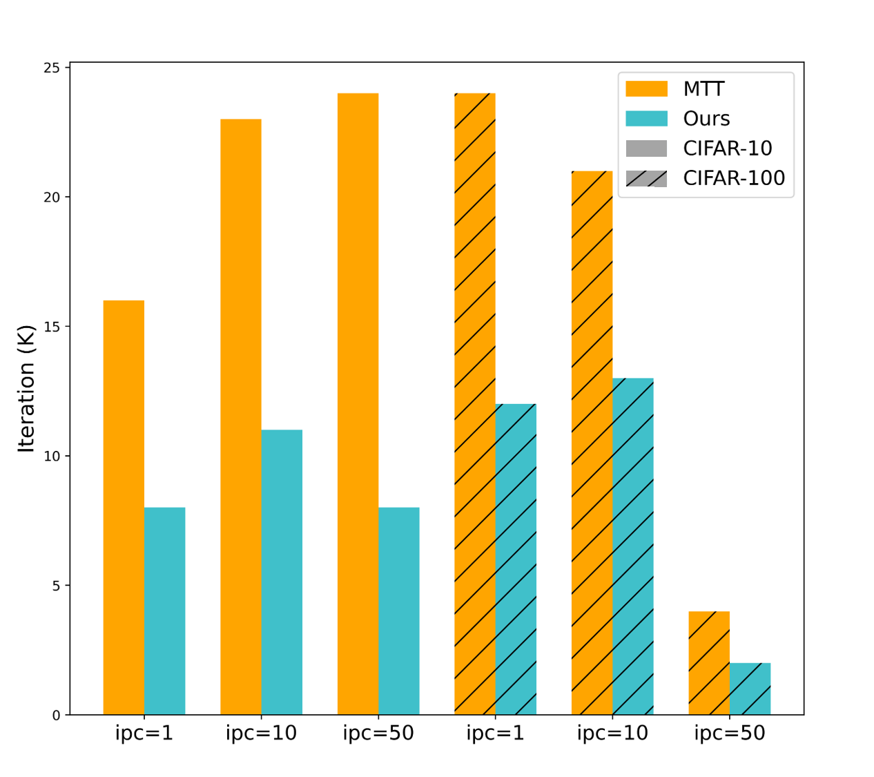
(b) Illustration of Convergence Speed

Figure 1: (a): PCA projection of all waypoints model in the expert trajectory, where z-axis represents the value of $(1-\text{validation accuracy})$; (b): The required iteration number to convergence for both the MCT and MTT methods during distillation. The convergence is defined by the condition where the difference between the accuracy at any iteration and the maximum accuracy is less than $\epsilon$=2%.

1. Instability of expert trajectory: As shown in Figure 1(a), the validation accuracy of the expert network on the MTT trajectory exhibits oscillations. Matching the trajectory locally in each iteration will lead to the similar oscillation in the trajectory of the synthetic data, thereby impeding robust distillation.

2. Low Convergence Speed: The learning process for the expert trajectory is often slow. As in Figure 1(b), a considerable number of distillation iterations are required to generate a synthetic dataset capable of achieving satisfactory test accuracy, resulting in time-consuming procedures.

3. High Storage Consumption: During the distillation process, the conventional MTT approach necessitates the storage of model weights along all timesteps, which is particularly burdensome in terms of storage (about 50 models should be stored). This high storage consumption is a significant limitation for applying existing DD methods to small-scale models.

Through careful observation, we have reformulated the loss function of MTT, and introduced a novel perspective to interpret the essence of DD and MTT: obtaining a synthetic dataset that offers accurate guidance regarding the magnitude and direction of the next update for any given point in the parameter space of the student model, with this guidance determined by the expert trajectory’s update vector at that point. From this perspective, those three limitations can be easily addressed: to find an optimized expert trajectory that can guide the model to stably converge at each iteration, which is also easy to fit and simple to save.

How to find such a trajectory? Drawing inspiration from linearized dynamics of Neural Tangent Kernel (NTK) method (Arora et al., 2019; Jacot et al., 2018), we present a simple yet novel Matching Convexified Trajectory (MCT) method. The MCT method creates a convex combination (linear) expert trajectory based on the network’s training process real data. This trajectory, which starts from a random initialization model and points directly towards the optimal model point, facilitates stable and rapid convergence of the distillation. Moreover, recovering this trajectory only needs storing two models and a set of constants. Distinct from the MTT method, the convexified trajectory also permits a “continuous sampling” strategy during the distillation, ensuring comprehensive learning and fitting of the expert trajectory.

The contributions of this paper are as follows: 1) We highlight the three limitations of traditional MTT methods, and offer a novel perspective for understanding the objective of DD through a simple reformulation of MTT’s loss function. 2) We propose the MCT method, which creates an easy-to-store convexified expert trajectory with a continuous sampling strategy to enable rapid and stable distillation. 3) Comprehensive experiments on three datasets have verified the superiority of our MCT and the effectiveness of the continuous sampling strategy.

2 Preliminaries and Related Work

2.1 Preliminaries

We first formally define the dataset distillation task. A large scale real dataset $\mathcal{T}=\{(x^{(i)}_{\mathcal{T}},y^{(i)}_{\mathcal{T}})\}_{i=1}^{|\mathcal{T}|}$ is first provided, where $x^{(i)}_{\mathcal{T}}\in\mathbb{R}^{d}$ and $y^{(i)}_{\mathcal{T}}\in\mathcal{Y}=\{1,2,\dots,C\}$ are the $i$-th instance and the corresponding label. $C$ denotes the number of classes. The core idea of this task is to learn a tiny synthetic dataset $\mathcal{S}=\{(x^{(i)}_{\mathcal{S}},y^{(i)}_{\mathcal{S}})\}_{i=1}^{|\mathcal{S}|}$ from the original dataset $\mathcal{T}$, where $x^{(i)}_{\mathcal{S}}\in\mathbb{R}^{d}$ and $y^{(i)}_{\mathcal{S}}\in\mathcal{Y}$. Typically, $ipc$ instances are crafted for each class, culminating in a total count for $\mathcal{S}$ of ${|\mathcal{S}|}=C*ipc$. It is always expected that ${|\mathcal{S}|}\ll{|\mathcal{T}|}$, while $\mathcal{S}$ still preserves the majority of the pivotal information in $\mathcal{T}$. Consequently, a model trained on $\mathcal{S}$ should achieve performance comparable to the model trained with the original dataset $\mathcal{T}$ under the real data distribution $\mathcal{P}_{D}$. Formally, the optimization of DD task can be formulated as:

$$\arg\min_{\mathcal{S}}\mathcal{L}(\mathcal{S},\mathcal{T}),$$ (1)

where $\mathcal{L}$ is the certain objective function, which may differ from different DD methods.

2.2 Dataset Distillation Methods.

The field of DD contains four principal approaches. a. Meta-model Matching methods (Wang et al., 2018; Zhou et al., 2022; Nguyen et al., 2021; Loo et al., 2022) involve a bi-level optimization algorithm where the inner loop updates the weights of a differentiable model using gradient descent on a synthetic dataset while caching recursive computation graphs, and the outer loop validates models trained in the inner loops on a real dataset, back-propagating the validation loss through the unrolled computation graph to the synthetic dataset. b. Distribution Matching methods (Zhao and Bilen, 2023; Wang et al., 2022) align synthetic and real data by optimizing within a set of embedding spaces using maximum mean discrepancy. However, inaccurate estimation of the data distribution often results in suboptimal performance. c. Single-step Gradient Matching methods (Zhao et al., 2020; Zhao and Bilen, 2021) aim to align the gradient of the synthetic dataset with that of the real dataset during each training step. To enhance generalization with improved gradients, recent research efforts have focused on further optimizing the gradient matching objective by incorporating class-related information (Lee et al., 2022; Jiang et al., 2023). d. Multi-step Trajectory Matching methods (Cazenavette et al., 2022; Guo et al., 2023) address the accumulated trajectory errors of single-step methods by matching the multi-step training trajectories of models separately trained on synthetic and real datasets.

Our research primarily focuses on multi-step trajectory matching methods. The first method in this branch is MTT (Cazenavette et al., 2022). Based on MTT, Du et al. (2023) presented to incorporate the random noise to the initialized model weights to mitigate accumulated trajectory errors, and Cui et al. (2023) proposed to decompose the objective function of MTT to improve computational efficiency and reduce GPU memory without performance degradation. Further research has explored the robustness of the synthesized dataset (Guo et al., 2023; Li et al., 2022b; Du et al., 2024) and applied this technique to downstream tasks (Li et al., 2022a, 2020).

Despite their successes, none of these approaches address the detriment of oscillations in the MTT expert trajectory on the stability and convergence speed of the distillation process. Furthermore, the necessity to retain all waypoint networks along the expert trajectory has yet to be addressed.

3 Motivation

3.1 Review of Multi-step Trajectory Matching

In this section, we first review the multi-step trajectory matching methods. The essence of them is to minimize the discrepancy of the student training trajectory of $\mathcal{S}$ and the expert training trajectory of $\mathcal{T}$. Here we take MTT (Cazenavette et al., 2022) as an example. Firstly, an expert trajectory $\tau_{\text{mtt}}=\{\theta_{\mathcal{T}}^{(t)}|0\leq t\leq K\}$ is generated by training a randomly initialized model $\theta_{\mathcal{T}}^{(0)}$ on the real dataset $\mathcal{T}$ with $K$ timesteps. Afterward, MTT matches the student trajectory with the expert $\tau_{\text{mtt}}$ through massive iterations. During each iteration, MTT samples a random timestep $\theta^{(t)}_{\mathcal{T}}$ and captures the target timestep $\theta^{(t+M)}_{\mathcal{T}}$ after $M$ steps from $\tau_{\text{mtt}}$. Meanwhile, $\theta^{(t)}_{\mathcal{T}}$ is also trained on synthetic dataset $\mathcal{S}$ for $N$ steps to get the updated student parameters $\theta^{(t+N)}_{\mathcal{S}}$. Formally, the objective is to minimize the normalized squared $L_{2}$ error between the updated student parameters $\theta^{(t+N)}_{\mathcal{S}}$ and the future expert (target) parameters $\theta^{(t+M)}_{\mathcal{T}}$:

$$\mathcal{L}(\mathcal{S},\mathcal{T})=\frac{\|\theta^{(t+N)}_{\mathcal{S}}-\theta^{(t+M)}_{\mathcal{T}}\|^{2}_{2}}{\|\theta^{(t)}_{\mathcal{T}}-\theta^{(t+M)}_{\mathcal{T}}\|^{2}_{2}}$$ (2)

$$\theta_{\mathcal{S}}^{(t+1)}=\theta_{\mathcal{S}}^{(t)}-\alpha_{\mathcal{S}}\nabla\ell(\mathcal{S};\theta_{\mathcal{S}}^{(t)})$$ (3)

$$\theta_{\mathcal{T}}^{(t+1)}=\theta_{\mathcal{T}}^{(t)}-\alpha_{\mathcal{T}}\nabla\ell(\mathcal{T};\theta_{\mathcal{T}}^{(t)}),$$ (4)

where $\theta_{\mathcal{T}}^{(t)}=\theta_{\mathcal{S}}^{(t)}$. $\ell$ is the loss function for model training, where the cross-entropy loss is often adopted, and $\alpha_{\mathcal{S}}$ and $\alpha_{\mathcal{T}}$ are the learning rates for training on the synthetic and real datasets, respectively. To ensure generalization, MTT usually performs the above trajectory matching process on a large number of expert trajectories from different $\theta_{\mathcal{T}}^{(0)}$. Although the subsequent methods have focused on optimizing model parameters (Du et al., 2023, 2024) and objective functions (Cui et al., 2023), the overall process remains roughly the same as MTT.

3.2 Motivation: A New Perspective to Optimize the Trajectory

Through a lot of preliminary experiments and visualizations, we found that the MTT method have three serious shortcomings: 1. Instability of the expert trajectory generated by mini-batch SGD: The expert trajectory $\tau_{\text{mtt}}$ trained on $\mathcal{T}$ exhibits erratic oscillations instead of following a path where the loss steadily decreases, so the accuracy of the waypoint model $\theta^{(t)}_{\mathcal{T}}$ is subject to fluctuations. This problem complicates the student network to learn better training dynamics with synthetic data. 2. Low convergence speed of the distillation process: When learning expert trajectories, a very large number of iterations are required to obtain a synthetic dataset that can achieve good validation accuracy, which is very time-consuming. 3. High storage consumption of the expert trajectory: To expedite the distillation process, the expert trajectories are pre-generated and stored in memory as trajectory buffers. These trajectories serve as sources from which the initial point $\theta^{(t)}_{\mathcal{T}}$ and target parameters $\theta^{(t+M)}_{\mathcal{T}}$ are extracted. However, the necessity to store all waypoints for each expert trajectory incurs a substantial storage footprint.

To better explain the internalization of these drawbacks, we propose a novel perspective to view the dataset distillation and explain the essence of the MTT approach: The objective of DD task can be regarded as obtaining a set of parameters (i.e., the synthetic dataset $\mathcal{S}$) that enables accurate prediction of how far (magnitude) and where (direction) to step next for any given network parameters $\theta$ (i.e., provides appropriate guidance $\vec{V}_{\mathcal{S}}$ to update the current network parameters $\theta$). From this perspective, each distillation iteration of the MTT method can be viewed as updating the synthetic dataset $\mathcal{S}$ to provide the network update guidance $\vec{V}_{\mathcal{S}}=\|\theta^{(t+N)}_{\mathcal{S}}-\theta^{(t)}_{\mathcal{T}}\|^{2}_{2}$ of $N$-step SGD training on $\mathcal{S}$, which aligns closer to the $M$-step SGD guidance $\vec{V}_{\mathcal{T}}=\|\theta^{(t+M)}_{\mathcal{T}}-\theta^{(t)}_{\mathcal{T}}\|^{2}_{2}$ obtained from the expert trajectory, given an arbitrary initialized point $\theta_{\mathcal{T}}^{(t)}$. A simple reformulation of Equ. 2 yields the same result:

$$\min_{\mathcal{S}}\mathcal{L}(\mathcal{S},\mathcal{T})=\min_{\mathcal{S}}\mathbb{E}_{\theta^{(t)}_{\mathcal{T}}\sim\tau_{\text{mtt}}}\frac{\|(\theta^{(t+N)}_{\mathcal{S}}-\theta^{(t)}_{\mathcal{T}})-(\theta^{(t+M)}_{\mathcal{T}}-\theta^{(t)}_{\mathcal{T}})\|^{2}_{2}}{\|\theta^{(t)}_{\mathcal{T}}-\theta^{(t+M)}_{\mathcal{T}}\|^{2}_{2}}=\min_{\mathcal{S}}\mathbb{E}_{\theta^{(t)}_{\mathcal{T}}\sim\tau_{\text{mtt}}}\frac{\left\|\vec{V}_{\mathcal{S}}-\vec{V}_{\mathcal{T}}\right\|^{2}_{2}}{\left\|\vec{V}_{\mathcal{T}}\right\|^{2}_{2}},\\$$ (5)

Thereafter, we can regard all the waypoints of $\tau_{\text{mtt}}$ as the training “dataset” to optimize $\vec{V}_{\mathcal{S}}$, i.e., ${\{(\theta^{(t)}_{\mathcal{T}},\vec{V}^{(t)}_{\mathcal{T}})|\theta^{(t)}_{\mathcal{T}}\in\tau_{\text{mtt}},0\leq t\leq K\}}$, where $\vec{V}^{(t)}_{\mathcal{T}}$ denotes the “label” of $\theta^{(t)}_{\mathcal{T}}$. From this perspective, the first two drawbacks can be easily explained: Given that the models on the expert trajectory $\tau_{\text{mtt}}$ are all obtained by SGD training, and considering the variations in sample distribution across mini-batches, the expert trajectory $\tau_{\text{mtt}}$ has huge oscillations. Therefore, the training dynamics $\vec{V}^{(t)}_{\mathcal{T}}$ obtained by sampling two arbitrary points with an interval of $M$ steps from $\tau_{\text{mtt}}$ cannot guarantee to always provide a favorable direction for $\vec{V}^{(t)}_{\mathcal{S}}$ to learn. The final result is 1) poor $\vec{V}^{(t)}_{\mathcal{T}}$ leads to instability; 2) considerable time is expended in identifying the optimal optimization direction to achieve convergence. This raises the question: Is there a superior trajectory $\hat{\tau}$ that consistently delivers more advantageous $\vec{V}^{(t)}_{\mathcal{T}}$ to optimize the synthetic dataset $\mathcal{S}$ through $\vec{V}^{(t)}_{\mathcal{S}}$?

We believe that an ideal expert trajectory should: 1) For any $\hat{\theta}_{\mathcal{T}}^{(t)}$ on $\hat{\tau}$, the obtained $\vec{V}^{(t)}_{\mathcal{T}}$ should always point to the direction that guides the target loss $\ell(\mathcal{T};\theta_{\mathcal{T}}^{(t)})$ to decrease; 2) This trajectory is easier to fit for $\mathcal{S}$, because the size of $\mathcal{S}$ is much smaller than the original dataset $\mathcal{T}$. 3) The trajectory is easy to save and restore.

We draw inspiration from convex optimization (Boyd and Vandenberghe, 2004; Bubeck, 2015) and NTK (Jacot et al., 2018; Hanin and Nica, 2019). First, since deep learning is essentially a non-convex problem, if we can make expert trajectories exhibit more convex properties, optimization becomes much less difficult. How to find convex trajectories? NTK methods prove that for a neural network $f_{\theta}(x)$, its update can be approximated by its first-order Taylor expansion in the neural network tangent space (Lee et al., 2019):

$$f_{\theta}(x)\approx f_{lin,\theta}(x)=f_{\theta_{0}}(x)+(\theta-\theta_{0})^{\mathsf{T}}\nabla_{\theta}f_{\theta_{0}}(x).$$ (6)

From this, we believe that replacing the original trajectory with a convex combination (linear) trajectory would be much more effective. The starting and ending points of this linear trajectory are the same as $\tau_{\text{mtt}}$, and all the waypoints are distributed along this line. This trajectory meets our needs very well: 1) The visualization in Figure 1(a) verifies that the validation accuracy of the model on this trajectory consistently increases; 2) The direction of any $\vec{V}^{(t)}_{\mathcal{T}}$ sampled from this trajectory is always from the starting point to the ending (optimal) point, which is easy to fit for distilled data; 3) Only the parameters of its starting and ending points need to be stored, and the trajectory can be reconstructed by linear interpolation; 4) This trajectory is continuous, rather than consisting of intermittently sampled points like the original path, which greatly enriches our training set.

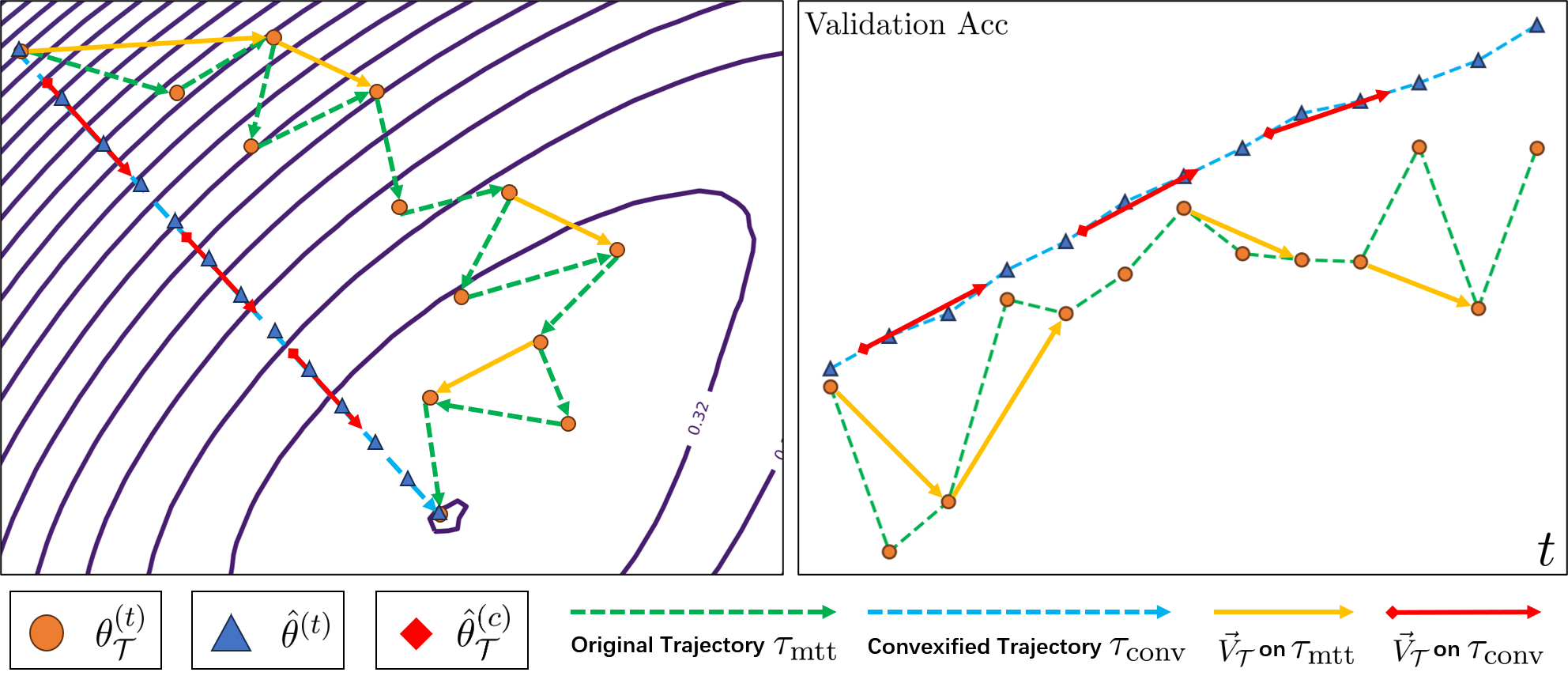
Figure 2: An illustration of the proposed MCT method. The left figure illustrates a schematic of the landscape in the model parameter space, while the right figure shows the validation accuracy of waypoint models extracted from expert trajectories of both the MTT method and our MCT method. In the left figure, the original trajectory $\tau_{\text{mtt}}$ exhibits constant oscillations, causing $\vec{V}^{(t)}_{\mathcal{T}}$ to continuously change, resulting in fluctuating accuracy of the expert model in the right figure. In contrast, the trajectory $\tau_{\text{conv}}$ of our MCT method is very stable, thereby ensuring a consistent guidance direction, which leads to a steady improvement of the expert model as shown in the right figure.

4 Our proposed MCT Method

4.1 Matching Convexified Trajectory

The expert trajectory $\tau_{\text{mtt}}$ is pre-generated with the parameter of all waypoint models stored in memory, i.e., $\tau_{\text{mtt}}=\{\theta^{(0)}_{\mathcal{T}},\theta^{(1)}_{\mathcal{T}},\dots,\theta^{(t)}_{\mathcal{T}},\dots,\theta^{(K)}_{\mathcal{T}}\}$, where $\theta^{(t)}_{\mathcal{T}}$ is computed by multiple steps of mini-batch SGD (Cazenavette et al., 2022).

However, the trajectory generated by vanilla mini-batch SGD exhibits strong non-convexity, which makes synthetic data challenging to converge to an optimal solution. To this end, we proposed MCT, which creates a convexified trajectory $\tau_{\text{conv}}$ and is defined as:

$$\tau_{\text{conv}}=\{\hat{\theta}^{(t)}|0\leq t\leq K\},$$ (7)

$$\hat{\theta}^{(t)}=(1-\beta^{(t)}){\theta}^{(0)}_{\mathcal{T}}+\beta^{(t)}{\theta}^{(K)}_{\mathcal{T}},$$ (8)

where $\beta^{(t)}\in(0,1)$ is a weight value that determines the distribution of all waypoints. The starting point $\hat{\theta}^{(0)}$ and ending point $\hat{\theta}^{(K)}$ are same as ${\theta}^{(0)}_{\mathcal{T}}$ and ${\theta}^{(K)}_{\mathcal{T}}$ in $\tau_{\text{conv}}$. Particularly, the generated trajectory $\tau_{\text{conv}}$ directly points from ${\theta}^{(0)}_{\mathcal{T}}$ to ${\theta}^{(K)}_{\mathcal{T}}$, and $\beta^{(t)}$ is determined by the ratio of the difference between ${\theta}^{(t-1)}_{\mathcal{T}}$ and ${\theta}^{(t)}_{\mathcal{T}}$ in $\tau_{\text{mtt}}$ to the total length of $\tau_{\text{mtt}}$ as:

$$\begin{split}\beta^{(0)}&=0,\\ \beta^{(t)}&=\frac{\sum_{l=0}^{t-1}{\mathrm{Norm}(\theta_{\mathcal{T}}^{(l+1)}-\theta_{\mathcal{T}}^{(l)})}}{\sum_{l=0}^{K-1}{\mathrm{Norm}(\theta_{\mathcal{T}}^{(l+1)}-\theta_{\mathcal{T}}^{(l)})}},t=1,2,\dots,K,\end{split}$$ (9)

where $\mathrm{Norm}(\cdot)$ is $L_{2}$ norm. To mitigate discrepancies among different network layers, we calculate the $L_{2}$ normalization for each layer individually, i.e., $\beta^{(t)}=[\beta^{(t)}_{1},\beta^{(t)}_{2},\dots,\beta^{(t)}_{n}]^{\mathsf{T}}$, where each element in $\beta^{(t)}$ represents the weight value of a network layer. Note that our trajectory is generated based on $\tau_{\text{mtt}}$, and the calculation of $\beta^{(t)}$ does not require saving all the intermediate models ${\theta}^{(t)}_{\mathcal{T}}$. It only needs to save $\mathrm{Norm}(\theta_{\mathcal{T}}^{(l+1)}-\theta_{\mathcal{T}}^{(l)})$ obtained in each step of the expert trajectory $\tau_{\text{mtt}}$, allowing $\beta^{(t)}$ to be calculated at the end of expert training. Given this expert trajectory $\tau_{\text{conv}}$, the distillation in Equ. 2 can be conducted. During distillation, our MCT method always provides a convexified guidance $\vec{{V}}^{(t)}_{\mathcal{T}}$ with the direction from ${\theta}^{(0)}_{\mathcal{T}}$ to ${\theta}^{(K)}_{\mathcal{T}}$, leading to the steady optimization of $\vec{{V}}^{(t)}_{\mathcal{S}}$, and thus, the convergence of $\mathcal{S}$ will be rapid.

4.2 Continuous Sampling

Due to the continuity of our convexified trajectory, we can perform continuous sampling from the trajectory during distillation. This approach is completely different from the MTT method, enabling the selection of intermediate positions such as "the 1.5th point." Specifically, the MTT method only performs discrete sampling on the expert trajectory (i.e., selecting ${\theta}^{(t)}_{\mathcal{T}}$ with an integer $t$ ). In contrast, for $\tau_{\text{conv}}$ with the starting point $\hat{\theta}^{(0)}$ and ending point $\hat{\theta}^{(K)}$, since all points are on a straight line, we can obtain any timestep $\hat{\theta}^{(c)}$ with a decimal $c\in[0,K]$ on this line by interpolation:

$$\begin{split}\hat{\theta}^{(c)}&=(1-\hat{\beta})\hat{\theta}^{(0)}+\hat{\beta}\hat{\theta}^{(K)},\\ \hat{\beta}&=(1-\eta)\beta^{(\lfloor c\rfloor)}+\eta\beta^{(\lceil c\rceil)},\\ \eta&=c-\lfloor c\rfloor,\end{split}$$ (10)

After $\hat{\theta}^{(c)}$ and $\hat{\theta}^{(c+M)}$ are obtained, the distillation process can be conducted. This continuous sampling strategy ensures sufficient learning and fitting of the entire expert trajectory $\tau_{\text{conv}}$, facilitating thorough learning of the synthetic dataset $\mathcal{S}$.

4.3 Memory-Efficient Storage

In conventional MTT, the learning of the expert trajectory requires storing the parameters of all timesteps in memory, which will incur significant storage overhead. Formally, let $W$ denote the size of the network parameter $\theta^{(t)}_{\mathcal{T}}$ and $C$ denote the size of other irrelevant parameters. Since there are $K$ timesteps on $\tau_{\text{mtt}}$, the entire required storage will be:

$$\text{Storage}_{\text{mtt}}=K\times W+C=O(KW).$$ (11)

In contrast, our method only requires storing the starting point $\hat{\theta}^{(0)}$, the ending point $\hat{\theta}^{(K)}$, and point distribution $\{\beta^{(t)}|0\leq t\leq K\}$ along the trajectory. Therefore, the entire storage cost becomes:

$$\text{Storage}_{\text{conv}}=2\times W+K\times(\beta^{(t)})+C.$$ (12)

Since $\beta^{(t)}$ is a floating-point number, the storage cost will be $\text{Storage}_{\text{conv}}=O(W)$. In practice, $K$ is usually set to 50. Once the surrogate models in distillation become complex (e.g. LLMs), $K$ and $W$ will increase simultaneously, highlighting the significant storage advantages of our MCT method.

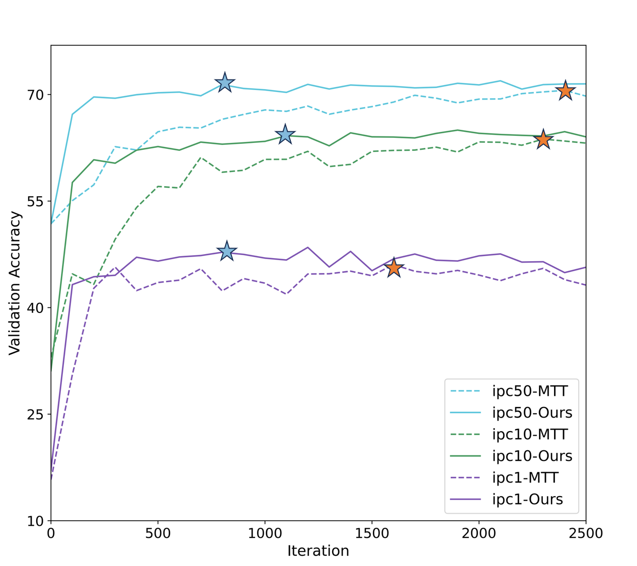
(a) Convergence on CIFAR-10

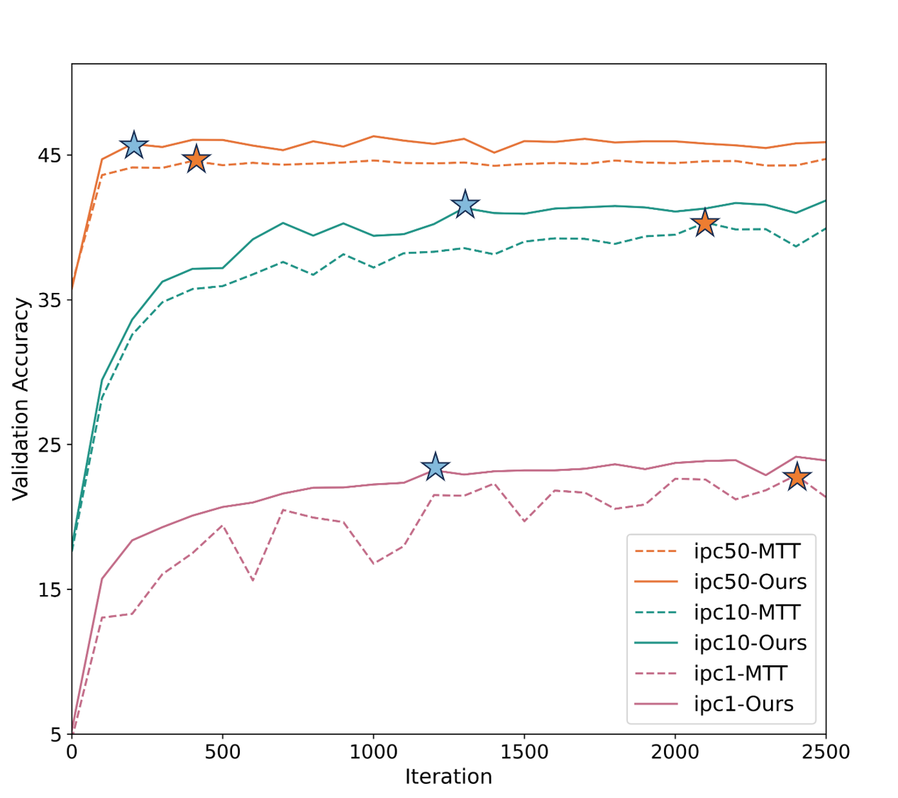
(b) Convergence on CIFAR-100

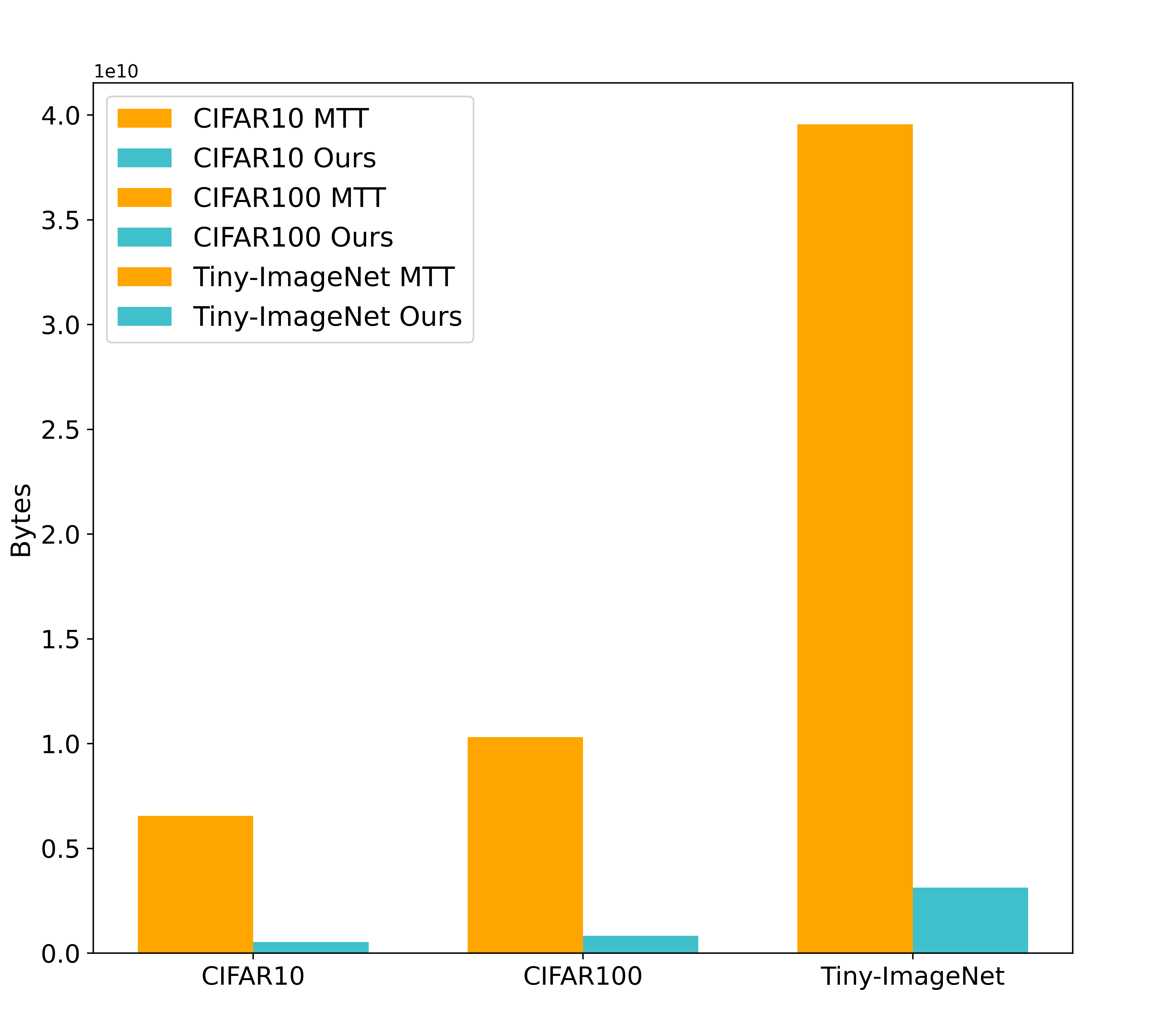
(c) Storage Comparison

Figure 3: (a) and (b): Convergence comparisons of distillation process on CIFAR-10 and CIFAR-100, where the symbol “star” denotes the convergence point. (c): Storage comparisons on three datasets.

5 Experiment

5.1 Experiment Setup

Experiment Settings: We evaluated our method on three datasets: CIFAR-10 and CIFAR-100 (Krizhevsky et al., 2009), and Tiny-ImageNet (Le and Yang, ). We first generated the convexified trajectories with our MCT method. Similar to MTT, we applied Kornia (Riba et al., 2020) Zero component analysis (ZCA) whitening on CIFAR-10, CIFAR-100, and Tiny-ImageNet datasets, and utilized Differentiable Siamese Augmentation (DSA) (Zhao and Bilen, 2021) technique during training and evaluation.

Evaluation and Baselines: Our MCT method is compared with several baselines from different branches, including Dataset Condensation (DC) (Zhao et al., 2020), Distribution Matching (DM) (Zhao and Bilen, 2023), DSA (Zhao and Bilen, 2021), Condense Aligning FEatures (CAFE) Wang et al. (2022), dataset distillation using Parameter Pruning (PP) (Li et al., 2023), and MTT. Following the conventional settings, we conducted dataset distillation using 1/10/50 images per class (ipc) for evaluations, respectively. The images with the resolution of 32 × 32 and 64 × 64 were synthesized on the CIFAR and Tiny-ImageNet datasets, respectively. Subsequently, five randomly initialized networks were trained in 1000 iterations with the cross-entropy loss on the distilled dataset. These trained networks were then evaluated on the real validation set, and their average accuracy (Acc) was reported as the evaluation metric. To maintain consistency with MTT and DC, we use ConvNet (Gidaris and Komodakis, 2018) as the surrogate model. This model comprises 128 filters with a 3 × 3 kernel size. Following the filters, instance normalization (Ulyanov et al., 2016) and ReLU activation are applied. Additionally, an average pooling layer with a kernel size of 2 × 2 and a stride of 2 is incorporated into the network.

Implementation Details: We adopt the same settings of MTT in most cases. Specifically, 100 expert trajectories are generated, each spanning 50 epochs of training (i.e., 51 timesteps). In practice, we often insert two waypoint models in the expert trajectory of MTT to derive our convexified trajectory: the models of 6-th and 25-th epochs for CIFAR-10 and the models of 15-th and 30-th epochs for CIFAR-100 and Tiny-ImageNet. During the distillation process, 5,000 distillation iterations are conducted. For each iteration, $\hat{\theta}^{(c)}$ is generated from Equ. 10, where the decimal $c$ is randomly sampled within [0, MaxStartEpoch]. We adopt the SGD optimizer, and a learnable learning rate is employed to distill the synthetic data. All experiments are run on four RTX3090 GPUs.

Table 1: Performance of Various Algorithms on Different Datasets

Dataset	CIFAR-10			CIFAR-100			Tiny ImageNet
ipc	1	10	50	1	10	50	1	10	50
Random	15.4±0.3	31.0±0.5	50.6±0.3	4.2±0.3	14.6±0.5	33.4±0.4	1.4±0.1	5.0±0.2	15.0±0.4
DC (Zhao et al., 2020)	28.3±0.5	44.9±0.5	53.9±0.5	12.8±0.3	25.2±0.3	-	-	-	-
DSA (Zhao and Bilen, 2021)	28.8±0.7	52.1±0.5	60.6±0.5	13.9±0.3	32.3±0.3	42.8±0.4	-	-	-
CAFE (Wang et al., 2022)	30.3±1.1	46.3±0.6	55.5±0.6	12.9±0.3	27.8±0.3	37.9±0.3	-	-	-
DM (Zhao and Bilen, 2023)	26.0±0.8	48.9±0.6	63.0±0.4	11.4±0.3	29.7±0.3	43.6±0.4	3.9±0.2	12.9±0.4	24.1±0.3
PP (Li et al., 2023)	46.4±0.6	65.5±0.3	71.9±0.2	24.6±0.1	43.1±0.3	48.4±0.3	-	-	-
MTT (Cazenavette et al., 2022)	46.3±0.8	65.3±0.7	71.6±0.2	24.3±0.3	40.1±0.4	47.7±0.2	8.8±0.3	23.2±0.2	28.0±0.3
Ours	48.5±0.2	66.0±0.3	72.3±0.3	24.5±0.5	42.5±0.5	46.8±0.2	9.6±0.5	22.6±0.8	27.6±0.4
Full dataset	84.8±0.1			56.2±0.3			37.6±0.4

5.2 Experiment Result

Validation Accuracy Comparison. Table 1 presents a comparison of validation accuracy between our method and various baselines across three datasets. Although performance is not the main focus of our MCT method, it is evident that our method achieves the best performance on the three metrics of the CIFAR-10 dataset as well as the ipc=1 metric of the Tiny ImageNet dataset. Notably, compared to the crucial MTT method, our MCT method demonstrates performance improvements in most metrics, indicating that our convexified trajectory and continuous sampling strategy can indeed provide enhanced guidance to the optimization of synthetic datasets.

Convergence of Distillation Process. Figure 3(a) and 3(b) illustrate the distillation processes utilizing the MCT and MTT methods for the CIFAR-10 and CIFAR-100 datasets. After every 100 distillation iterations, five networks with random initialization are trained on the current distillation dataset and their average accuracy on the validation set are recorded. The figures present the validation accuracy trends of both methods over the initial 2,500 iterations. As depicted, under all ipc settings, our MCT method achieves a substantial performance much sooner (200-1200 iterations ahead), indicating a faster convergence speed; after nearing convergence, the performance of the MCT method remains consistently stable as iterations proceed, whereas the MTT method still experiences significant performance fluctuations. These two phenomena suggest that our method effectively enhances training stability and accelerates the convergence process.

Comparison of Storage Requirement. Figure 3(c) compares the required storage of the expert trajectory between MTT and our MCT method. As demonstrated in Sec. 4.3, it is clear that our convex trajectories require significantly less memory (approximately 8%) compared to the expert trajectories needed by the MTT method. It is foreseeable that as model sizes and expert trajectories continue to grow, the space savings offered by our method will become even more substantial.

Visualization of Distilled Data. The visualization results of the synthetic data on CIFAR-10 with ipc=10 and CIFAR-100 with ipc=1 are presented in Figure 5(a) and 5(b). As we can see, the synthetic set learned from our expert trajectories exhibits notable degrees of recognizability and authenticity, while it also tends to integrate various characteristic features of images within the same category.

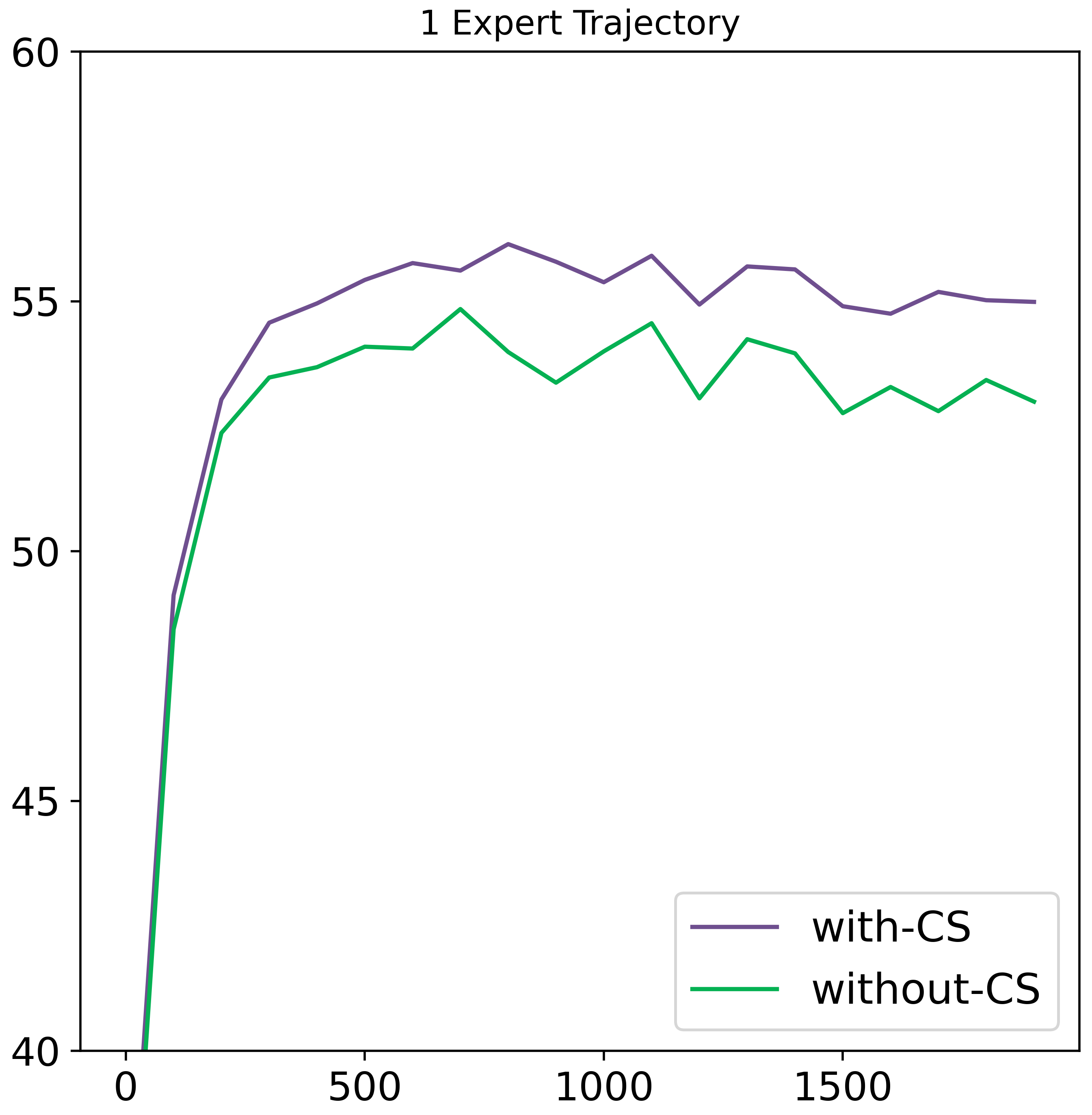
(a) 1 Expert Trajectory

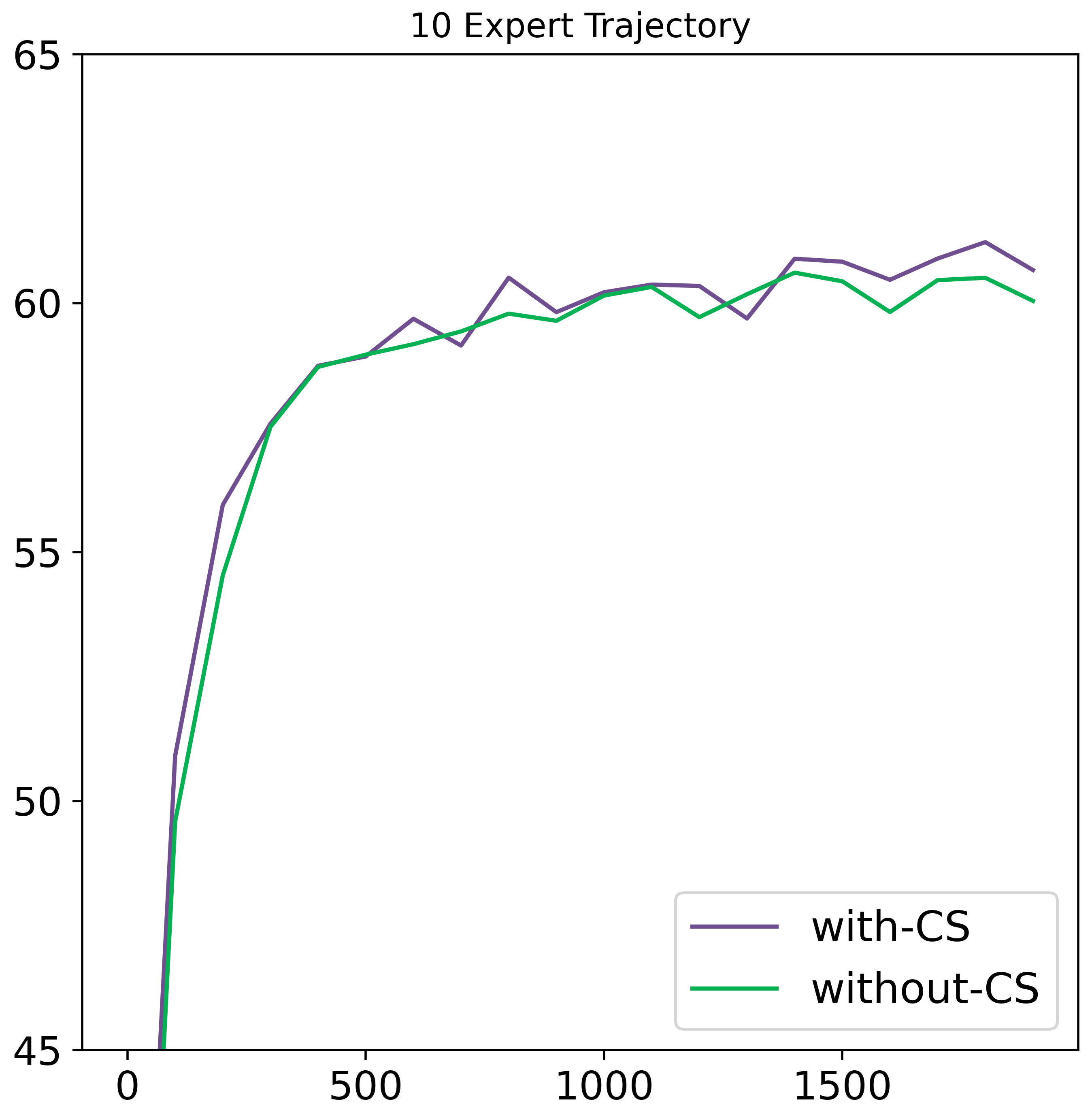
(b) 10 Expert Trajectories

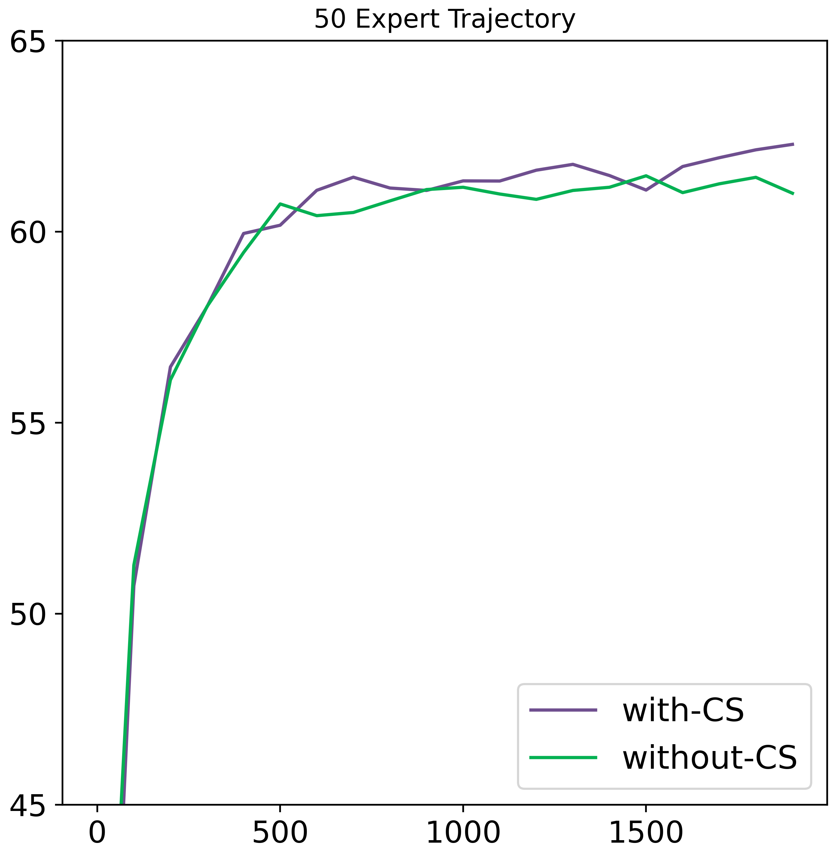
(c) 50 Expert Trajectories

Figure 4: Effects of Continuous Sampling over iterations with different expert trajectory numbers.

5.3 Ablation Studies

Table 2: Effects of Continuous Sampling with different numbers of expert trajectories on CIFAR-10.

Number of expert trajectories	1	5	10	20	50
w/o. Continuous Sampling	54.8±0.2	60.6±0.2	61.5±0.3	62.3±0.3	62.1±0.4
w. Continuous Sampling	56.2±0.3	61.3±0.5	61.8±0.6	62.8±0.3	62.8±0.2

Table 3: Effects of different $M$ with different ipc on CIFAR-10.

$M$	3	4	5	6	7
ipc=1	46.7	47.1	48.5	48.0	45.6
ipc=10	62.3	62.6	65.0	66.0	65.2
ipc=50	70.0	71.4	71.8	72.3	71.8

Effects of Continuous Sampling. To verify the effect of the continuous sampling, we set ipc=10 and randomized the starting epoch parameter within the range [0,5] on the CIFAR-10 dataset. The validation accuracy over iterations and the optimal accuracy throughout the entire distillation process are reported in Figure 4(c) and Table. 2, respectively. Overall, the integration of continuous sampling can improve the validation performance under all conditions. Moreover, the fewer the number of expert trajectories, the more pronounced the performance improvement brought about by the continuous sampling strategy. Those results prove that our continuous sampling can effectively expand the sampling space, ultimately leading to the enhancement of the final distillation outcomes.

Effects of expert updating step $M$. Table 3 shows the effects of the updating step $M$ of the expert trajectory $\tau_{\text{conv}}$ on the CIFAR-10 dataset. $N$ is set to 50 for all results. As we can see, when ipc=1, the optimal performance can be obtained at $M$=5, while when ipc=10 and ipc=50, the optimal performance can be obtained at $M$=6. Overall, our MCT method is robust to the selection of $M$ and will not experience significant performance degradation with changes in $M$.

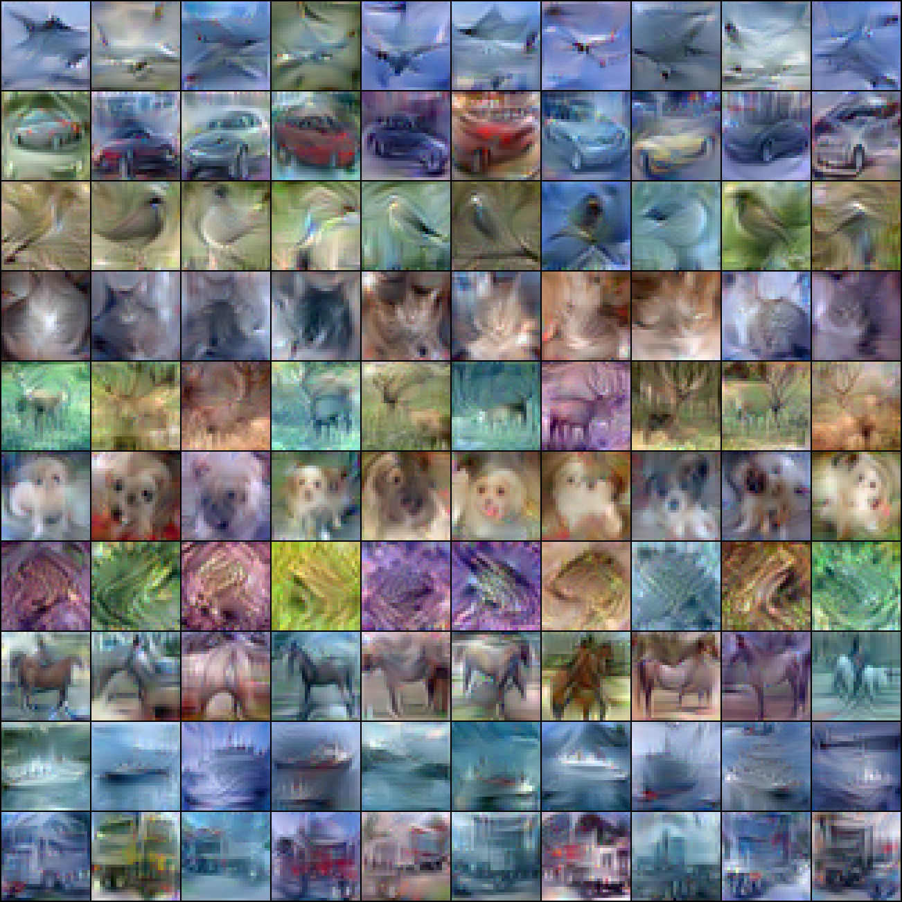
(a) CIFAR-10, ipc=10

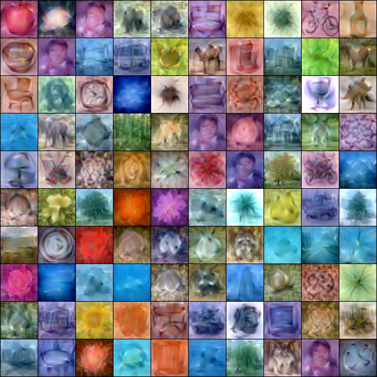
(b) CIFAR-100, ipc=1

Figure 5: Visualization of synthetic dataset.

6 Conclusion

To address three major limitations of traditional MTT, this paper draws inspiration from NTK methods and proposes a novel perspective to understand the essence of dataset distillation and MTT. A simple yet novel Matching Convexified Trajectory method is introduced to create a simplified, convexified expert trajectory that enhances the optimization process, leading to more stable and rapid convergence and reduced memory consumption. The convexified trajectory allows for continuous sampling during distillation, enriching the learning process and ensuring thorough fitting of the expert trajectory. Our experiments on CIFAR-10, CIFAR-100, and Tiny-ImageNet datasets demonstrate MCT’s superiority over MTT and other baselines. MCT’s ablation studies confirm the benefits of continuous sampling and the impact of the convexified trajectory on distillation performance. The results indicate that MCT is a promising solution for training complex models with reduced data needs, offering an efficient, stable, and memory-friendly approach to dataset distillation.

7 Limitations

Our MCT method has three primary limitations: 1. Although MCT can effectively enhance training stability and convergence speed, the improvement in validation accuracy is not very significant due to the starting and ending points being the same as those in MTT, and the enhancement is mainly attributed to the more thorough trajectory learning enabled by continuous sampling; future work could identify better endpoints to further improve performance. 2. While our trajectory provides a direction with more stable and rapidly descending, the calculation the magnitude $\beta$ is relatively simple (derived by the proportion of MTT step size to trajectory length), and there may exist more optimal step sizes that allow for more rapid and robust trajectory learning. 3. The linear approximation of NTK is proposed based on infinitely wide networks and requires some rather strict initialization methods. However, we did not conduct our work under this condition; further theoretical deduction is required to address this issue.

References

- Arora et al. [2019] Sanjeev Arora, Simon S Du, Wei Hu, Zhiyuan Li, Russ R Salakhutdinov, and Ruosong Wang. On exact computation with an infinitely wide neural net. Advances in neural information processing systems, 32, 2019.
- Boyd and Vandenberghe [2004] Stephen Boyd and Lieven Vandenberghe. Convex Optimization. Cambridge University Press, 2004.
- Bubeck [2015] Sébastien Bubeck. Convex optimization: Algorithms and complexity, 2015.
- Cazenavette et al. [2022] George Cazenavette, Tongzhou Wang, Antonio Torralba, Alexei A Efros, and Jun-Yan Zhu. Dataset distillation by matching training trajectories. In Proceedings of the IEEE/CVF Conference on Computer Vision and Pattern Recognition, pages 4750–4759, 2022.
- Cui et al. [2023] Justin Cui, Ruochen Wang, Si Si, and Cho-Jui Hsieh. Scaling up dataset distillation to imagenet-1k with constant memory. In International Conference on Machine Learning, pages 6565–6590. PMLR, 2023.
- Du et al. [2023] Jiawei Du, Yidi Jiang, Vincent YF Tan, Joey Tianyi Zhou, and Haizhou Li. Minimizing the accumulated trajectory error to improve dataset distillation. In Proceedings of the IEEE/CVF Conference on Computer Vision and Pattern Recognition, pages 3749–3758, 2023.
- Du et al. [2024] Jiawei Du, Qin Shi, and Joey Tianyi Zhou. Sequential subset matching for dataset distillation. Advances in Neural Information Processing Systems, 36, 2024.
- Gidaris and Komodakis [2018] Spyros Gidaris and Nikos Komodakis. Dynamic few-shot visual learning without forgetting. In Proceedings of the IEEE conference on computer vision and pattern recognition, pages 4367–4375, 2018.
- Guo et al. [2023] Ziyao Guo, Kai Wang, George Cazenavette, Hui Li, Kaipeng Zhang, and Yang You. Towards lossless dataset distillation via difficulty-aligned trajectory matching. arXiv preprint arXiv:2310.05773, 2023.
- Hanin and Nica [2019] Boris Hanin and Mihai Nica. Finite depth and width corrections to the neural tangent kernel. arXiv preprint arXiv:1909.05989, 2019.
- Jacot et al. [2018] Arthur Jacot, Franck Gabriel, and Clément Hongler. Neural tangent kernel: Convergence and generalization in neural networks. Advances in neural information processing systems, 31, 2018.
- Jiang et al. [2023] Zixuan Jiang, Jiaqi Gu, Mingjie Liu, and David Z Pan. Delving into effective gradient matching for dataset condensation. In 2023 IEEE International Conference on Omni-layer Intelligent Systems (COINS), pages 1–6. IEEE, 2023.
- Krizhevsky et al. [2009] Alex Krizhevsky, Geoffrey Hinton, et al. Learning multiple layers of features from tiny images. 2009.
- [14] Ya Le and Xuan Yang. Tiny imagenet visual recognition challenge.
- Lee et al. [2019] Jaehoon Lee, Lechao Xiao, Samuel Schoenholz, Yasaman Bahri, Roman Novak, Jascha Sohl-Dickstein, and Jeffrey Pennington. Wide neural networks of any depth evolve as linear models under gradient descent. Advances in neural information processing systems, 32, 2019.
- Lee et al. [2022] Saehyung Lee, Sanghyuk Chun, Sangwon Jung, Sangdoo Yun, and Sungroh Yoon. Dataset condensation with contrastive signals. In International Conference on Machine Learning, pages 12352–12364. PMLR, 2022.
- Li et al. [2020] Guang Li, Ren Togo, Takahiro Ogawa, and Miki Haseyama. Soft-label anonymous gastric x-ray image distillation. In 2020 IEEE International Conference on Image Processing (ICIP), pages 305–309. IEEE, 2020.
- Li et al. [2022a] Guang Li, Ren Togo, Takahiro Ogawa, and Miki Haseyama. Compressed gastric image generation based on soft-label dataset distillation for medical data sharing. Computer Methods and Programs in Biomedicine, 227:107189, 2022a.
- Li et al. [2022b] Guang Li, Ren Togo, Takahiro Ogawa, and Miki Haseyama. Dataset distillation for medical dataset sharing. arXiv preprint arXiv:2209.14603, 2022b.
- Li et al. [2023] Guang Li, Ren Togo, Takahiro Ogawa, and Miki Haseyama. Dataset distillation using parameter pruning. IEICE Transactions on Fundamentals of Electronics, Communications and Computer Sciences, 2023.
- Loo et al. [2022] Noel Loo, Ramin Hasani, Alexander Amini, and Daniela Rus. Efficient dataset distillation using random feature approximation. Advances in Neural Information Processing Systems, 35:13877–13891, 2022.
- Nguyen et al. [2021] Timothy Nguyen, Roman Novak, Lechao Xiao, and Jaehoon Lee. Dataset distillation with infinitely wide convolutional networks. Advances in Neural Information Processing Systems, 34:5186–5198, 2021.
- Riba et al. [2020] Edgar Riba, Dmytro Mishkin, Daniel Ponsa, Ethan Rublee, and Gary Bradski. Kornia: an open source differentiable computer vision library for pytorch. In Proceedings of the IEEE/CVF Winter Conference on Applications of Computer Vision, pages 3674–3683, 2020.
- Ulyanov et al. [2016] Dmitry Ulyanov, Andrea Vedaldi, and Victor Lempitsky. Instance normalization: The missing ingredient for fast stylization. arXiv preprint arXiv:1607.08022, 2016.
- Wang et al. [2022] Kai Wang, Bo Zhao, Xiangyu Peng, Zheng Zhu, Shuo Yang, Shuo Wang, Guan Huang, Hakan Bilen, Xinchao Wang, and Yang You. Cafe: Learning to condense dataset by aligning features. In Proceedings of the IEEE/CVF Conference on Computer Vision and Pattern Recognition, pages 12196–12205, 2022.
- Wang et al. [2018] Tongzhou Wang, Jun-Yan Zhu, Antonio Torralba, and Alexei A Efros. Dataset distillation. arXiv preprint arXiv:1811.10959, 2018.
- Zhao and Bilen [2021] Bo Zhao and Hakan Bilen. Dataset condensation with differentiable siamese augmentation. In International Conference on Machine Learning, pages 12674–12685. PMLR, 2021.
- Zhao and Bilen [2023] Bo Zhao and Hakan Bilen. Dataset condensation with distribution matching. In Proceedings of the IEEE/CVF Winter Conference on Applications of Computer Vision, pages 6514–6523, 2023.
- Zhao et al. [2020] Bo Zhao, Konda Reddy Mopuri, and Hakan Bilen. Dataset condensation with gradient matching. In International Conference on Learning Representations, 2020.
- Zhou et al. [2022] Yongchao Zhou, Ehsan Nezhadarya, and Jimmy Ba. Dataset distillation using neural feature regression. Advances in Neural Information Processing Systems, 35:9813–9827, 2022.