CERN-TH-2024-089, P3H-24-041, TTP24-020, ZU-TH 30/24
Nonleptonic $B$-meson decays to next-to-next-to-leading order

Abstract

We compute next-to-next-to-leading order QCD corrections to the partonic processes $b\to c\bar{u}d$ and $b\to c\bar{c}s$, which constitute the dominant decay channels in standard model predictions for $B$-meson lifetimes within the heavy quark expansion. We consider the contribution from the four-quark operators $O_{1}$ and $O_{2}$ in the $\Delta B=1$ effective Hamiltonian. The decay rates are obtained from the imaginary parts of four-loop propagator-type diagrams. We compute the corresponding master integrals using the “expand and match” approach which provides semi-analytic results for the physical charm and bottom quark masses. We show that the dependence of the decay rate on the renormalization scale is significantly reduced after including the next-to-next-to-leading order corrections. Furthermore, we compute next-to-next-to-leading order corrections to the Cabibbo-Kobayashi-Maskawa-suppressed decay channels $b\to u\bar{c}s$ and $b\to u\bar{u}d$.

1 Introduction

Bound states of quarks and anti-quarks in the form of hadrons are commonly observed in collider experiments. Their lifetimes are among the most important quantities to obtain insights into the fundamental interactions of elementary particles. In this paper we consider $B$ mesons which contain a heavy $b$ quark or anti-quark and a lighter quark $u,d$ or $s$. Their decay is governed by the weak interaction of the $b$ quark. The theoretical framework describing the decay rates of inclusive decays of hadrons containing a heavy quark is the heavy quark expansion (HQE). Lifetimes, which are the inverse of the total decay width, can be calculated in the HQE as a double series expansion in $\Lambda_{\mathrm{QCD}}/m_{b}$ and the strong coupling constant $\alpha_{s}$. The first term in the $\Lambda_{\mathrm{QCD}}/m_{b}$ expansion describes the decay of a free bottom quark within perturbative QCD (for reviews see [1, 2]). The leading term is complemented by power-suppressed contributions involving matrix elements of higher-dimensional operators. Global fits [3, 4] of $B\to X_{c}\ell\bar{\nu}_{\ell}$ data measured at $B$ factories provide the numerical values for the matrix elements involving two-quark operators, like the kinetic and chromo-magnetic terms $\mu_{\pi}^{2}$ and $\mu_{G}^{2}$. Lifetimes depend also on matrix elements of four-quark operators, which can be estimated by HQET sum rules [5, 6] or calculated on the lattice [7, 8].

At leading order in $\Lambda_{\mathrm{QCD}}/m_{b}$, the total decay width $\Gamma(B_{q})$ is given by the sum of the semileptonic decay channels $b\to c\ell\bar{\nu}_{\ell}$, with $\ell=e,\mu,\tau$, the nonleptonic channels $b\to c\bar{u}d$, $b\to c\bar{u}s$, $b\to c\bar{c}d$ and $b\to c\bar{c}s$, as well as other CKM suppressed and rare decay modes. For reviews we refer to Refs. [1, 2]. Next-to-next-to-leading order (NNLO) corrections to the semi-leptonic decay rate have been computed a few years ago [9, 10, 11, 12]. More recently also the $O(\alpha_{s}^{3})$ corrections [13, 14] became available, even for the kinematic moments without experimental cuts [15].

The nonleptonic decays of $B$ mesons are most conveniently described with the help of the $\Delta B=1$ effective Hamiltonian [16, 17] governing the low-energy dynamics at the renormalization scale $\mu_{b}\sim m_{b}$. For them only next-to-leading order (NLO) corrections are currently available [18, 19, 20, 21, 22, 23, 24]. At NNLO there are only partial results from Ref. [25] where only one of the relevant four-quark operators has been considered. Furthermore, no resummation of the large logarithms $\log(M_{W}/m_{b})$ due to the running from the electroweak scale to the scale of the $B$ meson mass has been performed.

On the basis of all currently available correction terms, one obtains the following results for the $B$ meson decay rates [26]

$$\Gamma(B^{+}) = 0.58^{+0.11}_{-0.07}\,\mbox{ps}^{-1}\,,$$

$$\Gamma(B_{d}) = 0.63^{+0.11}_{-0.07}\,\mbox{ps}^{-1}\,,$$ (1)

with an uncertainly of almost 20%. It is by far dominated by the renormalization scale dependence of the free-quark decay. The uncertainties arising from CKM elements and quark mass values are significantly smaller. For this reason, the current state-of-the-art calls for a determination of NNLO corrections to nonleptonic decays in the free quark approximation, including an appropriate choice of the short-distance mass scheme for the heavy quarks. In this work, we aim to address this gap by providing results for the NNLO corrections to the nonleptonic decay of a free quark, where the charm and bottom quark masses are renormalized on-shell. We take into account finite charm and bottom quark masses and consider the so-called current-current operators $O_{1}$ and $O_{2}$, which provide the dominant contribution to the decay width. We will show that the $\mu_{b}$ dependence is significantly reduced once the NNLO corrections are included. For an update of the decay widths in Eq. (1) it is necessary to consider other renormalization schemes for the quark masses. Furthermore, one has to properly combine all decay channels and incorporate the known power-suppressed terms [27, 28, 29, 30, 31, 32]. This is postponed to a future publication [33].

The paper is organised as follows: In Section 2 we set up the notation, introduce the effective Hamiltonian and the operators $O_{1}$ and $O_{2}$. We discuss in particular how to apply naive dimensional regularization and use anticommuting $\gamma_{5}$. This is crucial in order to adopt the same prescription utilized in the calculation of the NNLO anomalous dimensions of $O_{1}$ and $O_{2}$ [16, 34]. The detail of the calculation of interference terms up to $O(\alpha_{s}^{2})$ and the evaluation of the four-loop master integrals are presented in Section 3. We also discuss in details the role of evanescent operators in the calculation. In Section 4 we combine our predictions for the squared amplitudes up to $O(\alpha_{s}^{2})$ with the NNLO Wilson coefficients evaluated at the low-scale $\mu_{b}\sim m_{b}$ and give results for the rate of the different channels. We conclude in Section 5. In the Appendix A, we provide additional details about the operator renormalization.

2 Framework

We describe the nonleptonic decays of a bottom quark governed by weak interactions using the effective Hamiltonian

$$\mathcal{H}_{\rm eff}=\frac{4G_{F}}{\sqrt{2}}\sum_{q_{1,3}=u,c}\sum_{q_{2}=d,s}\lambda_{q_{1}q_{2}q_{2}}\Big{(}C_{1}(\mu_{b})O_{1}^{q_{1}q_{2}q_{3}}+C_{2}(\mu_{b})O_{2}^{q_{1}q_{2}q_{3}}\Big{)}+{\rm h.c.}\,,$$ (2)

where $\lambda_{q_{1}q_{2}q_{3}}=V_{q_{1}b}V_{q_{2}q_{3}}^{\star}$ are the corresponding CKM matrix elements and $C_{i}(\mu_{b})$ are the Wilson coefficients for the $\Delta B=1$ effective operators evaluated at the renormalization scale $\mu_{b}\sim m_{b}$. The current-current operators $O_{i}^{q_{1}q_{2}q_{3}}$ are given by [16, 17]

$$O_{1}^{q_{1}q_{2}q_{3}} =(\bar{q}_{1}^{\alpha}\gamma^{\mu}P_{L}b^{\beta})(\bar{q}_{2}^{\beta}\gamma_{\mu}P_{L}q_{3}^{\alpha}),$$

$$O_{2}^{q_{1}q_{2}q_{3}} =(\bar{q}_{1}^{\alpha}\gamma^{\mu}P_{L}b^{\alpha})(\bar{q}_{2}^{\beta}\gamma_{\mu}P_{L}q_{3}^{\beta})\,,$$ (3)

where $\alpha$ and $\beta$ refer to colour indices. We will refer to such operator definition as the historical basis. For simplicity, we will ignore the penguin operators whose contributions to the rate are suppressed due to the numerically small Wilson coefficients. Another common operator choice is the so-called Chetyrkin-Misiak-Münz (CMM) basis [35], in which the operators are

$$O_{1}^{{}^{\prime}\,q_{1}q_{2}q_{3}} =(\bar{q}_{1}T^{a}\gamma^{\mu}P_{L}b)(\bar{q}_{2}T^{a}\gamma_{\mu}P_{L}q_{3}),$$

$$O_{2}^{{}^{\prime}\,q_{1}q_{2}q_{3}} =(\bar{q}_{1}\gamma^{\mu}P_{L}b)(\bar{q}_{2}\gamma_{\mu}P_{L}q_{3}),$$ (4)

where $T^{a}$ are the generator of the $SU(3)$ colour group. The CMM basis was introduced to consistently use fully anticommuting $\gamma_{5}$ at any number of loops in the evaluation of the QCD corrections to $b\to s\gamma$ and $b\to s\ell\ell$ decays. However, this feature breaks down for the processes considered in this article and the historical basis turns out to be more convenient for our calculation, as explained below. Moreover, the historical basis is the default choice in many phenomenological studies [1, 31, 26, 36, 2].

In our study, we treat the bottom and the charm quark as massive with mass $m_{b}$ and $m_{c}$, respectively, while all other quarks are considered massless ($m_{u,d,s}=0$). We then divide the nonleptonic decays into three classes based on the flavour indices of $O_{1}$ and $O_{2}$:

1. Three massless quarks in the final state, i.e.  $q_{1}q_{2}q_{3}=udu,usu$.

2. One charm quark and two massless quarks ($q_{1}q_{2}q_{3}=cdu,csu,udc,usc$).

3. Two charm quarks and one massless quark ($q_{1}q_{2}q_{3}=cdc$ and $csc$).

In the following, we will focus on the CKM-favoured decays $b\to c\bar{u}d$ and the CKM-suppressed mode $b\to u\bar{c}s$ as representatives for case (ii). For case (iii) we consider $b\to c\bar{c}s$. Case (i) can be obtained from the $m_{c}\to 0$ limit of the other two, however it requires the additional calculation of the finite charm-mass effect originating from closed charm-loop insertion into a gluon propagator (see the sample diagram in Fig. 1(i)). We will refer to this kind of effect as the $U_{c}$ contribution. Note also that our NNLO results will include (small) contributions associated to the production of an addition $\bar{c}c$ pair from gluon splitting, e.g. $b\to c\bar{u}d(g^{\star}\to\bar{c}c)$.

To calculate the inclusive decay width, we use the optical theorem and evaluate the imaginary part of forward scattering amplitudes for an on-shell bottom quark up to NNLO. For a definite flavour content of the operators, the contribution to the decay rate can be written as

$$\Gamma^{q_{1}q_{2}q_{3}}(\rho)=\frac{1}{m_{b}}\sum_{i,j=1,2}\left(\frac{4G_{F}|\lambda_{q_{1}q_{2}q_{3}}|}{\sqrt{2}}\right)^{2}\\ C_{i}^{\dagger}(\mu_{b})C_{j}(\mu_{b})\,{\rm Im}\,i\int{\rm d}^{4}x\,e^{{\rm i}qx}\,\bra{b}T\Big{\{}O_{i}^{\dagger\,q_{1}q_{2}q_{3}}(x)O_{j}^{q_{1}q_{2}q_{3}}(0)\Big{\}}\ket{b}\Bigg{|}_{q^{2}=m_{b}^{2}}\,,$$ (5)

where $\rho=m_{c}/m_{b}$. As a consequence, at LO the imaginary parts of two-loop diagrams have to be computed and at NLO and NNLO, three- and four-loop diagrams have to be considered, see Fig. 1. For $b\to c\bar{c}s$ and $b\to u\bar{u}d$, besides the corrections in which the LO diagram in Fig. 1(a) is dressed with additional gluon lines, there are also contributions at order $O(\alpha_{s})$ and $O(\alpha_{s}^{2})$ due to the insertions of the operators $O_{1,2}$ into penguin diagrams like Fig. 2. These kind of corrections of $O(\alpha_{s})$ were studied in [37, 38, 24] and shown to be numerically much smaller than the $O(\alpha_{s})$ corrections arising from diagrams like Fig. 1(b). We postpone the evaluation of this class of penguin-like diagrams to a subsequent publication since they require a special treatment of cut Feynman integrals.

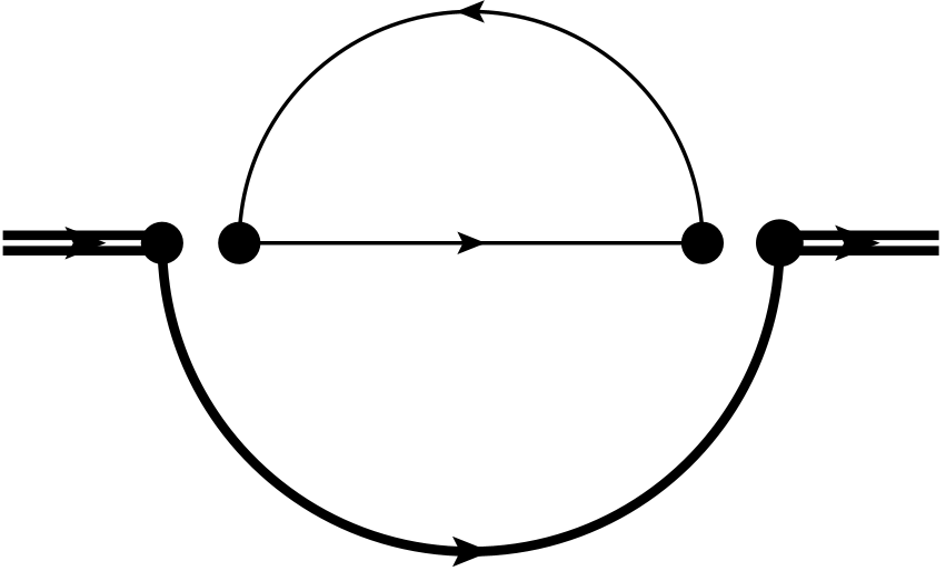
(a)

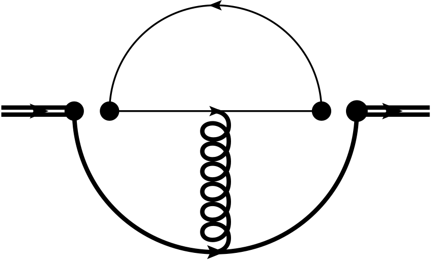
(b)

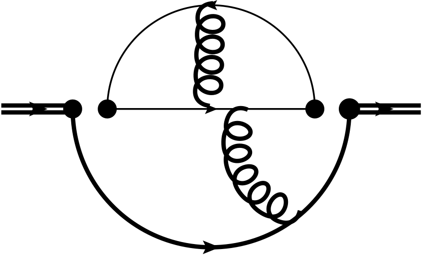
(c)

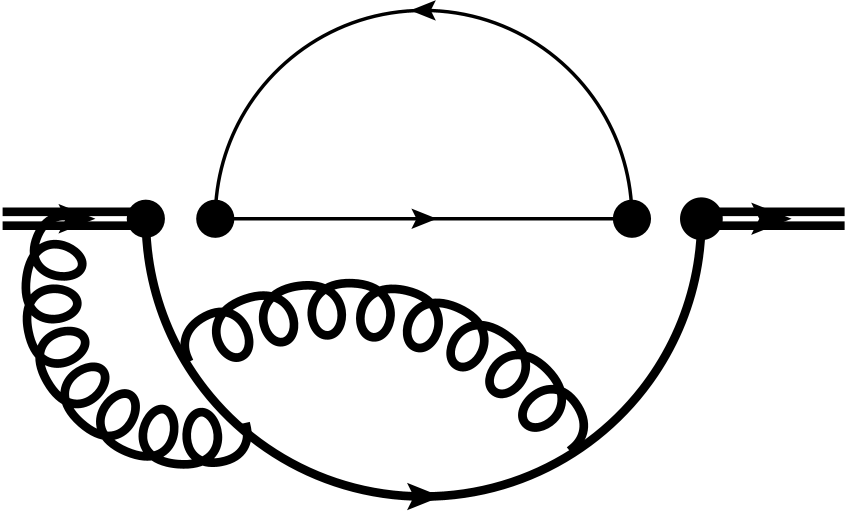
(d)

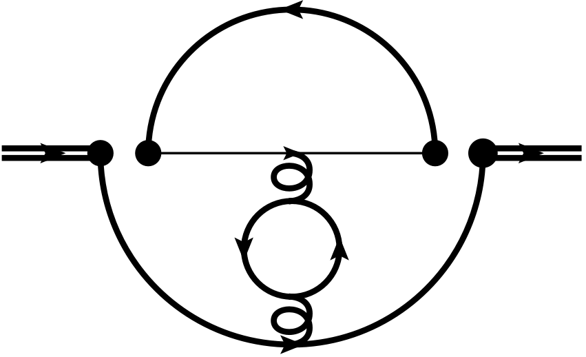
(e)

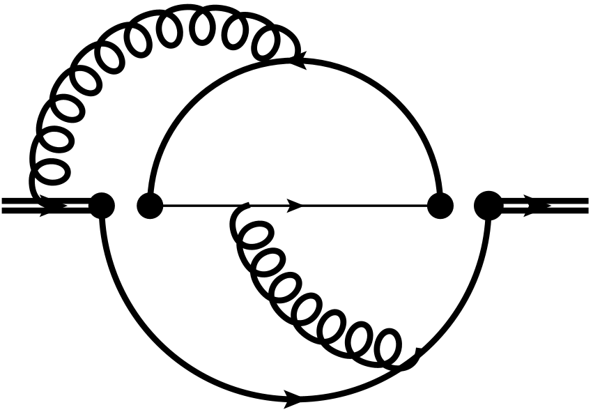
(f)

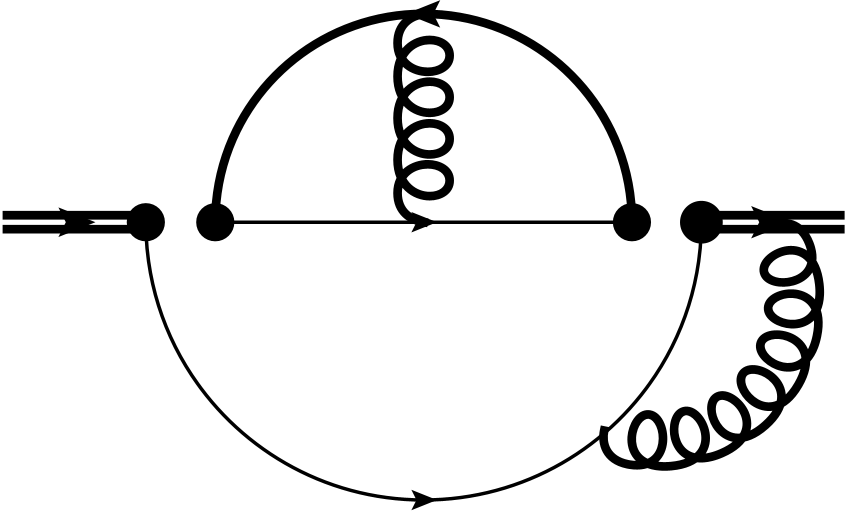
(g)

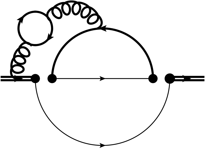
(h)

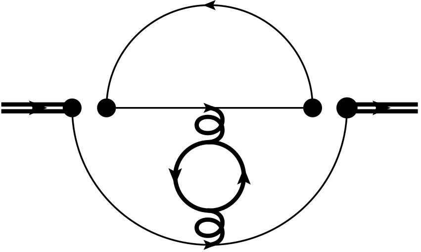
(i)

Figure 1: Example of Feynman diagrams contributing to the forward scattering amplitude in Eq. (5) at order $\alpha_{s}^{0}$ (LO), $\alpha_{s}$ (NLO) and $\alpha_{s}^{2}$ (NNLO). The dot pairs denote insertions of the effective operators and highlight how fermion flows are contracted. Thin, bold and double bold lines denote massless, charm and bottom propagators.

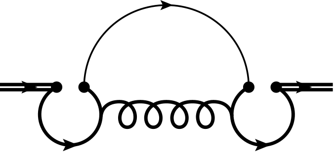
(a)

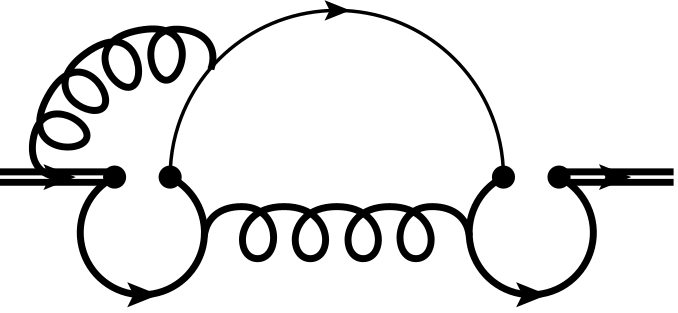
(b)

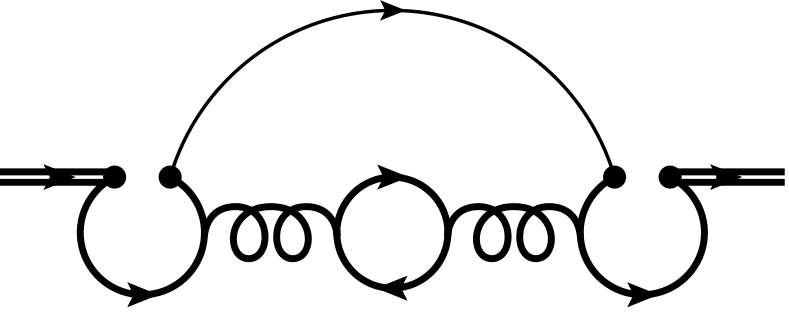
(c)

Figure 2: Example of Feynman diagrams with penguin topology at NLO and NNLO.

Due to the presence of $\gamma_{5}$ a straightforward use of naive dimensional regularization (NDR) is not possible. Starting from NLO there are traces with one $\gamma_{5}$ matrix that must be evaluated in $d=4-2\epsilon$ dimensions (see e.g. the diagram in Fig. 1(b)). For the calculation of the anomalous dimension (and thus the renormalization constants needed for the operator mixing) anticommuting $\gamma_{5}$ has been used [16, 34]. Thus we would like to apply the same prescription in our calculation.

In order to use anticommuting $\gamma_{5}$, we apply a method similar to the one discussed in Sec. 2.3 of Ref. [20]. Instead of Eq. (5), let us consider

$$\widetilde{\Gamma}^{q_{1}q_{2}q_{3}}(\rho)=\frac{1}{m_{b}}\sum_{i,j=1,2}\left(\frac{4G_{F}|\lambda_{q_{1}q_{2}q_{3}}|}{\sqrt{2}}\right)^{2}\\ \widetilde{C}_{i}^{\dagger}(\mu_{b})C_{j}(\mu_{b})\,{\rm Im}\,i\int{\rm d}^{4}x\,e^{{\rm i}qx}\bra{b}T\Big{\{}O_{i}^{q_{2}q_{1}q_{3}\,\dagger}(x)O_{j}^{q_{1}q_{2}q_{3}}(0)\Big{\}}\ket{b}\Bigg{|}_{q^{2}=m_{b}^{2}}\,.$$ (6)

Note the different ordering of the quark flavour indices in the first operator, i.e. $q_{2}q_{1}q_{3}$ instead of $q_{1}q_{2}q_{3}$. Here, $\widetilde{C}_{i}(\mu_{b})$ is the Wilson coefficient of the operator $O_{i}^{q_{2}q_{1}q_{3}}$. The forward scattering matrix defined by $\widetilde{\Gamma}^{q_{1}q_{2}q_{3}}$ leads to only one trace of gamma matrices containing an odd number of $\gamma_{5}$. This is easily seen from Fig. 3 where the effect is illustrated. Since the width is parity-even, the trace containing exactly one $\gamma_{5}$ can be discarded at any order in perturbation theory, while in case we encounter two $\gamma_{5}$ in the same trace we apply anticommuting $\gamma_{5}$. This means that for $\widetilde{\Gamma}^{q_{1}q_{2}q_{3}}$ we can use NDR and the renormalization constants known from the literature. If we had considered $\Gamma^{q_{1}q_{2}q_{3}}$, we would have encountered the product of two traces with one $\gamma_{5}$ each, which in general can give a parity-even contribution. This is shown in the NLO diagram on the left in Fig. 3.

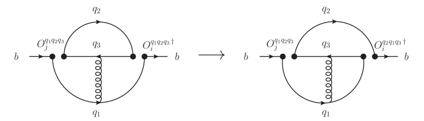
Figure 3: Illustration of the Fierz transformation on a diagram at NLO. In contrast to the diagram on the left contributing to $\Gamma^{q_{1}q_{2}q_{3}}$ in Eq. (5), the one on the right can be computed using anticommuting $\gamma_{5}$.

In the next step we recover the expression for $\Gamma^{q_{1}q_{2}q_{3}}$ from $\widetilde{\Gamma}^{q_{2}q_{1}q_{3}}$. In four dimensions the operators $O_{1}^{q_{2}q_{1}q_{3}}$ and $O_{2}^{q_{1}q_{2}q_{3}}$ are connected by a Fierz transformation:

$$O_{1}^{q_{1}q_{2}q_{3}} =(\bar{q}_{1}^{\alpha}\gamma^{\mu}P_{L}b^{\beta})(\bar{q}_{2}^{\beta}\gamma_{\mu}P_{L}q_{3}^{\alpha})=(\bar{q}_{2}^{\alpha}\gamma^{\mu}P_{L}b^{\alpha})(\bar{q}_{1}^{\beta}\gamma_{\mu}P_{L}q_{3}^{\beta})=O_{2}^{q_{2}q_{1}q_{3}},$$ (7)

and similarly $O_{2}^{q_{1}q_{2}q_{3}}=O_{1}^{q_{2}q_{1}q_{3}}$. This implies

$$\Gamma^{q_{1}q_{2}q_{3}}(\rho)=\widetilde{\Gamma}^{q_{2}q_{1}q_{3}}(\rho)\Big{|}_{\widetilde{C}_{1}\to C_{2},\,\widetilde{C}_{2}\to C_{1}}.$$ (8)

Fierz identities in general are not valid for $d\neq 4$, however, the Fierz symmetry can be restored order by order in perturbation theory by renormalization using anticommuting $\gamma_{5}$ and a suitable definition of the evanescent operators [16]. We will discuss in detail the renormalization and the evanescent operator scheme in section 3.3. In conclusion, our strategy for obtaining the NNLO prediction for $\Gamma^{q_{1}q_{2}q_{3}}$ is to calculate $\widetilde{\Gamma}^{q_{1}q_{2}q_{3}}$ and to adopt a renormalization scheme which preserves Eq. (8) up to $O(\alpha_{s}^{2})$.

3 Technical details

In this Section we provide details for the calculation of the squared amplitude, the master integrals and the renormalization scheme adopted for the effective operators in Eq. (3).

3.1 Generation of the amplitude

For our calculation we use a well-tested chain of programs which allows for a high degree of automation. We us qgraf [39] for the generation of the amplitude and tapir [40] for the translation to FORM [41] code and the identification of the underlying integral families. The program exp [42, 43] performs the mapping of the amplitudes to the integral families and prepares them for further processing with FORM. After applying projectors and decomposing the reducible numerator factors in terms of denominators, we obtain for each family a list of scalar integrals for which we need a reduction to so-called master integrals. For the decay channels with up to one charm quark in the final state at LO we perform the calculation for general QCD gauge parameter keeping linear terms and check that it drops out at the level of the renormalized amplitude. For the channel $b\to c\bar{c}s$ we choose Feynman gauge since the reduction is significantly more expensive.

We employ the program Kira [44] in combination with Fermat [45] and FireFly [46, 47]. for the reduction to master integrals, which is organised in two steps. First, we generate (for each family) reduction tables for seed integrals with up to two dots and one scalar product up to the top-level sector. These reduction tables serve as input for the program ImproveMasters.m [48] to search for a good basis, i.e. a master integral basis where the dependence on the kinematical quantity $\rho$ and on the dimension $d$ factorizes in all denominators. In the second step, we perform the reduction of the integrals needed for the amplitude onto the good basis that we found. We use Kira also for the minimization of the master integrals among all families. For the process $b\to c\bar{u}d$ we find 321, for $b\to c\bar{c}s$ 527 and for $U_{C}$ 21 master integrals. The calculation of the amplitudes for $b\to u\bar{c}s$ can be mapped to the same families as $b\to c\bar{u}d$.

3.2 Computation of the master integrals

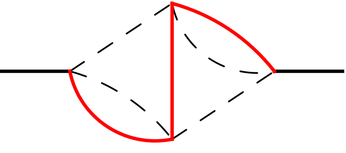
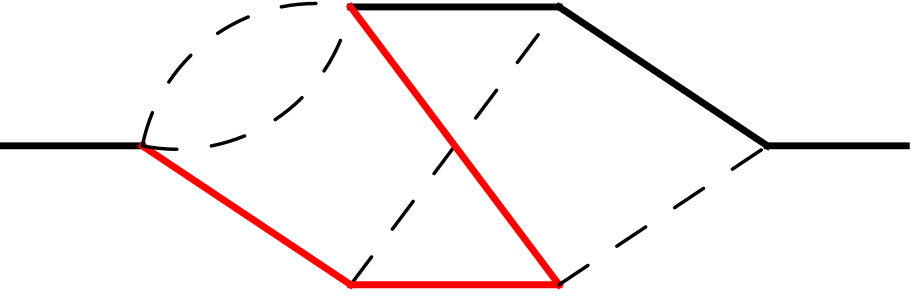
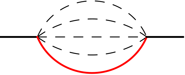
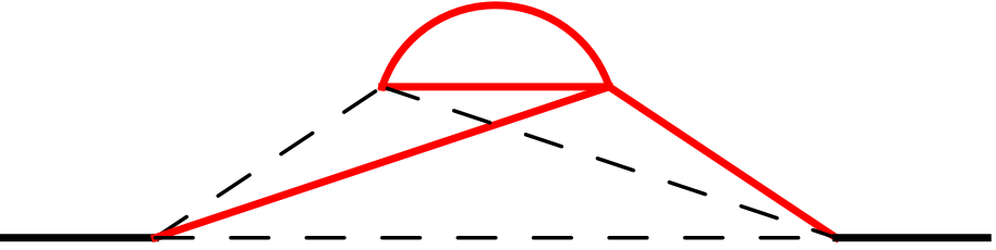
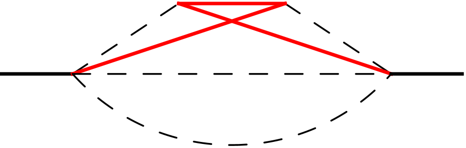
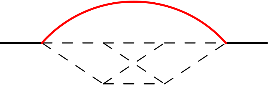
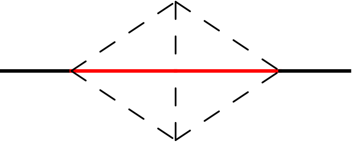
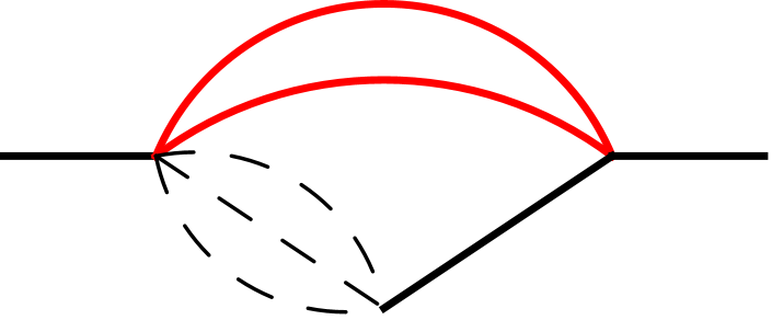
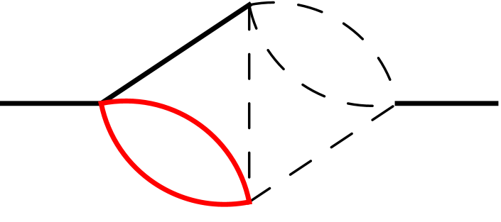
Figure 4: Samples of four-loop master integrals. Black and red solid lines represents massive propagator with mass $m_{b}$ and $m_{c}$, respectively, while dashed lines are massless propagators.

The master integrals at LO and NLO are calculated analytically. For both channels $b\to c\bar{u}d$ and $b\to c\bar{c}s$, we establish a set of differential equations for the master integrals by differentiating them with respect to $\rho$. Afterwards, we use the programs Canonica [49] and Libra [50] (the latter implements Lee’s algorithm [51]) to find a suitable basis transformation such that the masters in the new basis satisfy a set of differential equations in canonical form [52]. The boundary conditions to the differential equations are obtained using the auxiliary mass flow method [53, 54] as implemented in AMFlow [55]. We numerically compute all master integrals at NLO at a regular value of $\rho$ with about 150 digits, a precision sufficient to reconstruct the boundary constants in terms of transcendental numbers using the PSLQ algorithm [56]. The master integrals for $b\to c\bar{u}d$ are expressed through simple Harmonic Polylogarithms (HPLs) [57] with $\rho$ as argument. For the decay $b\to c\bar{c}s$, we apply the change of variable

$$\rho=\frac{x}{1+x^{2}},$$ (9)

to bring the system in canonical form. The solution is expressed in terms of iterated integrals over the letters $x,1+x,1-x,1+x^{2},1-x+x^{2}$ and $1+x+x^{2}$, which are also known as cyclotomic harmonic polylogarithms [58]. After factorizing the letters over the complex numbers, we can express the results in terms of generalized polylogarithms (GPLs) [59, 60].

At four-loop order we exclusively use the “expand and match” method [61, 62, 63, 64] which provides semi-analytic results for the master integrals in the form of expansions around properly chosen points with numerical coefficients. We use “expand and match” at LO and NLO as cross check for the analytic result. At NNLO the application to the subset of master integrals which already contribute the semileptonic decay rate is described in detail in Ref. [65]. In the following we concentrate on a brief summary and on the additional features present in the hadronic decay rate. In principle we could concentrate on the physical region with $m_{c}/m_{b}\approx 0.3$. However, for $b\to c\bar{u}d$ and $U_{C}$ we want to cover the whole region for $0\leq m_{c}/m_{b}\leq 1$ so that our results can also be applied to other physical situations. In the case of $b\to c\bar{c}s$, which is computationally much more demanding, we construct expansions which provide precise results for $0\leq m_{c}/m_{b}\lesssim 0.4$.

One of the ingredients for “expand and match” are the differential equations for the master integrals in the variable

$$\rho=\frac{m_{c}}{m_{b}}\,.$$ (10)

Let us stress that the system of differential equations does not have to be in a particular form; in particular it is not necessary to bring it into a canonical form [52, 51]. However, the computational time can be reduced in case the occurring denominators have a simple structure.

We denote the positions of the poles in the differential equation as singular points. In general, such branch cut points in the complex plane reflect physical thresholds. Some of the singularities are also spurious and no divergent behaviour is observed in the amplitude. All other points are called regular since there the master integrals have usual Taylor expansions.

As further ingredient, we need boundary conditions in the form of analytic or high-precision numerical results for the master integrals at a regular point of the differential equation. In our application we obtain the numerical boundary conditions with the help of AMFlow [55], typically requesting 80 digits. For $b\to c\bar{u}d$ we evaluate them for $\rho=1/4$, for $b\to c\bar{c}s$ at $\rho=1/5$ and $\rho=1/3$, and for $U_{C}$ at $\rho=1/3$.

The basic idea of “expand and match” is to construct truncated expansions around regular or singular points with the help of the differential equations and match them numerically at intermediate $\rho$-values. The first expansion point coincide with the value where the boundary conditions are computed.

At four-loop order we have singular points for those values of $\rho$ corresponding to the thresholds for the production of one, two, three or four charm quarks. For the various channels we have:

$$\rho_{\mathrm{singular}} \in\{0,1/3,1\} b\to c\bar{u}d\,,$$ for

$$\rho_{\mathrm{singular}} \in\{0,1/4,1/2\} b\to c\bar{c}s\,,$$ for

$$\rho_{\mathrm{singular}} \in\{0,1/2\} U_{C}\,.$$ for (11)

In the “expand and match” approach, usually the expansions around singular points are necessary in order to connect the solutions above and below the singularity. In order to improve the precision one can complement the list of expansion points by regular points. In our case we choose

$$\rho_{0}\in\{0,1/4,1/3,1/2,7/10,1\} \text{for }b\to c\bar{u}d\,,$$

$$\rho_{0}\in\{0,1/5,1/3\} \text{for }b\to c\bar{c}s\,,$$

$$\rho_{0}\in\{0,1/3,1/2,7/10,1\} \text{for }U_{C}\,.$$ (12)

The combination of the expansions provided for $b\to c\bar{u}d$ and $U_{C}$ lead to a precise covering of the whole range for $\rho\in[0,1]$. In the case of $b\to c\bar{c}s$ we can cover the physically interesting region $\rho\in[0.2,0.4]$ with high precision. Furthermore, as we will see below, both Taylor expansions agree at the singular point $\rho_{0}=1/4$ to about 15 digits and thus the computation of the expansions around $\rho_{0}=1/4$, which is computationally quite expensive, can be avoided for practical purposes. Nonetheless, also for $b\to c\bar{c}s$ we provide for convenience an expansion around the massless charm quark limit.

Let us briefly discuss the different ansätze which we have to use for the different expansion points. They have to incorporate the respective physical situation and contain logarithms and/or square roots.

For regular points $\rho_{0}$ the ansatz for the master integral $I_{i}$ is a simple Taylor expansion and it is given by

$$I_{i}(\rho,\epsilon) = \sum_{j=-4}^{\epsilon_{\mathrm{max}}}\sum_{n=0}^{n_{\mathrm{max}}}c_{i,j,n}\epsilon^{j}\left(\rho-\rho_{0}\right)^{n}\,.$$ (13)

For $\rho_{0}=0$ a power-log expansion is needed which we parametrize as

$$I_{i}(\rho,\epsilon) = \sum_{j=-4}^{\epsilon_{\mathrm{max}}}\sum_{m=0}^{j+4}\sum_{n=0}^{n_{\mathrm{max}}}c_{i,j,m,n}\epsilon^{j}\,(\rho-\rho_{0})^{n}\,\log^{m}\left(\rho-\rho_{0}\right)\,.$$ (14)

We can use this ansatz also for threshold singularities involving an odd number of particles. For an even number of cut particles, the ansatz has to contain also square roots [66] and reads

$$I_{i}(\rho,\epsilon) = \sum_{j=-4}^{\epsilon_{\mathrm{max}}}\sum_{m=0}^{j+4}\sum_{n=n_{\mathrm{min}}}^{n_{\mathrm{max}}}c_{i,j,m,n}\epsilon^{j}\,(\rho-\rho_{0})^{n/2}\,\log^{m}\left(\rho-\rho_{0}\right)\,.$$ (15)

We use this ansatz for $\rho_{0}=1/2$.

3.3 Renormalization

In the following we discuss the renormalization scheme adopted for the operators $O_{1}$ and $O_{2}$ to preserve the Fierz symmetry in Eq. (8) up to NNLO.

In a first step we perform the usual parameter renormalization for the strong coupling constant in the $\overline{\rm MS}$ scheme with five active flavours and the charm and bottom quark masses in the pole scheme. Furthermore, we also renormalize the wave function of the external bottom quark in the on-shell scheme. It is important to expand the bare two- and three-loop correlators to ${\cal O}(\epsilon^{2})$ and ${\cal O}(\epsilon)$, respectively, in order to obtain the correct constant terms at NNLO.

In a second step we take into account the counterterms originating from operator mixing (see Appendix A for details). This requires that in Eq. (6) not only the physical operators $O_{1}$ and $O_{2}$ are considered, but also evanescent operators [16, 67].

As shown in [16], Fierz symmetry can be restored order by order in perturbation theory by requiring that the anomalous dimension matrix (ADM) $\hat{\gamma}$, which governs the renormalization group evolution of the Wilson coefficients $C_{1}$ and $C_{2}$, namely

$$\mu_{b}\frac{\mathrm{d}C_{i}}{\mathrm{d}\mu_{b}}=\gamma_{ji}C_{j}\quad\text{for }i,j=1,2,$$ (16)

fulfils

$$\gamma_{11} =\gamma_{22}, \gamma_{12} =\gamma_{21}.$$ (17)

We expand the ADM in series of $\alpha_{s}$:

$$\hat{\gamma}=\hat{\gamma}^{(0)}\frac{\alpha_{s}(\mu_{b})}{4\pi}+\hat{\gamma}^{(1)}\left(\frac{\alpha_{s}(\mu_{b})}{4\pi}\right)^{2}+\hat{\gamma}^{(2)}\left(\frac{\alpha_{s}(\mu_{b})}{4\pi}\right)^{3}+O(\alpha_{s}^{4}).$$ (18)

The conditions (17) can be imposed order by order in $\alpha_{s}$ by a proper definition of the evanescent operators. At NLO, they are defined by [16]:

$$E_{1}^{(1),q_{1}q_{2}q_{3}} =(\bar{q}_{1}^{\alpha}\gamma^{\mu_{1}\mu_{2}\mu_{3}}P_{L}b^{\beta})(\bar{q}_{2}^{\beta}\gamma_{\mu_{1}\mu_{2}\mu_{3}}P_{L}q_{3}^{\alpha})-(16-4\epsilon)O_{1}^{q_{1}q_{2}q_{3}},$$

$$E_{2}^{(1),q_{1}q_{2}q_{3}} =(\bar{q}_{1}^{\alpha}\gamma^{\mu_{1}\mu_{2}\mu_{3}}P_{L}b^{\alpha})(\bar{q}_{2}^{\beta}\gamma_{\mu_{1}\mu_{2}\mu_{3}}P_{L}q_{3}^{\beta})-(16-4\epsilon)O_{2}^{q_{1}q_{2}q_{3}},$$ (19)

where we introduced the notation

$$\gamma^{\mu_{1}\dots\mu_{N}}=\gamma^{\mu_{1}}\dots\gamma^{\mu_{N}}.$$ (20)

While the $\epsilon$-independent term in front of $O_{1}$ and $O_{2}$ on the r.h.s. of (19) is unique and obtained by requiring that the evanescent operator vanishes for $d=4$, the coefficients of $O(\epsilon)$ and higher are in principle arbitrary. This leads to the well-known scheme dependence of the ADM starting at NLO, which eventually cancels for physical observables against the scheme dependence of the matching condition for the Wilson coefficients at the scale $\mu_{W}\simeq M_{W}$ and the matrix element of the effective operators at the low scale $\mu_{b}\sim m_{b}$. The definition in Eq. (19) leads to the NLO anomalous dimension matrix

$$\hat{\gamma}^{(1)}=\begin{pmatrix}-\frac{21}{2}-\frac{2}{9}n_{f}&\frac{7}{2}+\frac{2}{3}n_{f}\\[5.0pt] \frac{7}{2}+\frac{2}{3}n_{f}&-\frac{21}{2}-\frac{2}{9}n_{f}\end{pmatrix},$$ (21)

which preserves Fierz symmetry up to $O(\alpha_{s})$.

At NNLO we have to consider the following evanescent operators:

$$E_{1}^{(1),q_{1}q_{2}q_{3}} =(\bar{q}_{1}^{\alpha}\gamma^{\mu_{1}\mu_{2}\mu_{3}}P_{L}b^{\beta})(\bar{q}_{2}^{\beta}\gamma_{\mu_{1}\mu_{2}\mu_{3}}P_{L}q_{3}^{\alpha})-(16-4\epsilon+A_{2}\epsilon^{2})O_{1}^{q_{1}q_{2}q_{3}},$$

$$E_{2}^{(1),q_{1}q_{2}q_{3}} =(\bar{q}_{1}^{\alpha}\gamma^{\mu_{1}\mu_{2}\mu_{3}}P_{L}b^{\alpha})(\bar{q}_{2}^{\beta}\gamma_{\mu_{1}\mu_{2}\mu_{3}}P_{L}q_{3}^{\beta})-(16-4\epsilon+A_{2}\epsilon^{2})O_{2}^{q_{1}q_{2}q_{3}},$$

$$E_{1}^{(2),q_{1}q_{2}q_{3}} =(\bar{q}_{1}^{\alpha}\gamma^{\mu_{1}\mu_{2}\mu_{3}\mu_{4}\mu_{5}}P_{L}b^{\beta})(\bar{q}_{2}^{\beta}\gamma_{\mu_{1}\mu_{2}\mu_{3}\mu_{4}\mu_{5}}P_{L}q_{3}^{\alpha})-(256-224\epsilon+B_{1}\epsilon^{2})O_{1}^{q_{1}q_{2}q_{3}},$$

$$E_{2}^{(2),q_{1}q_{2}q_{3}} =(\bar{q}_{1}^{\alpha}\gamma^{\mu_{1}\mu_{2}\mu_{3}\mu_{4}\mu_{5}}P_{L}b^{\alpha})(\bar{q}_{2}^{\beta}\gamma_{\mu_{1}\mu_{2}\mu_{3}\mu_{4}\mu_{5}}P_{L}q_{3}^{\beta})-(256-224\epsilon+B_{2}\epsilon^{2})O_{2}^{q_{1}q_{2}q_{3}},$$ (22)

At $O(\alpha_{s}^{2})$ also $O(\epsilon^{2})$ terms must be considered in the coefficients multiplying $O_{1}^{q_{1}q_{2}q_{3}}$ and $O_{2}^{q_{1}q_{2}q_{3}}$ in the evanescent operator definitions. By imposing that also the NNLO ADM $\gamma^{(2)}$ fulfils Eq. (17), we can fix the coefficient $A_{2}$, $B_{1}$ and $B_{2}$. To this end, we take the expressions for $\gamma^{(2)}$ in the CMM basis [34] and perform a transformation to the historical basis. For simplicity we restrict ourself to $O_{1}$ and $O_{2}$, neglecting the penguin operators. We give more details on the basis transformation in the Appendix A. We find that the Fierz symmetry is preserved by a one-parameter class of renormalization scheme defined by:

$$B_{1} =-\frac{4384}{115}-\frac{32}{5}n_{f}+A_{2}\Bigg{(}\frac{10388}{115}-\frac{8}{5}n_{f}\Bigg{)},$$

$$B_{2} =-\frac{38944}{115}-\frac{32}{5}n_{f}+A_{2}\Bigg{(}\frac{19028}{115}-\frac{8}{5}n_{f}\Bigg{)}.$$ (23)

We highlight two notable scheme choices. The first one is

$$A_{2} =-4, B_{1} =-\frac{45936}{115}, B_{2} =-\frac{115056}{115},$$ (24)

which gives a definition of $E_{1,2}^{(2)}$ independent on $n_{f}$ however with $B_{1}\neq B_{2}$. We adopt the values in Eq. (24) as reference scheme for the evanescent operators. All scheme dependent quantities will be given relative to this choice. Another notable choice would be

$$A_{2} =+4, B_{1} =B_{2}=\frac{1616}{5}-\frac{64}{5}n_{f},$$ (25)

which leads to the same coefficient for $E_{1}^{(2)}$ and $E_{2}^{(2)}$ at $O(\epsilon^{2})$. In principle, we could have defined the evanescent operators $E_{1}^{(1)}$ and $E_{2}^{(1)}$ in a more general way with unequal coefficients at order $\epsilon^{2}$, namely with $A_{1}\neq A_{2}$. In this case one would find a class of renormalization schemes governed by two parameters instead of one. However we observe that the only solution independent on $n_{f}$ still correspond to the case given in Eq. (23), therefore for simplicity we set $A_{1}=A_{2}$, and verify that the dependence on $A_{2}$ drops out in the total width.

With the evanescent operator definition in Eq. (22), we compute at LO all correlators which involve $\{O_{1},O_{2},E_{1}^{(1)},E_{2}^{(1)},E_{1}^{(2)},E_{2}^{(2)}\}$ and at NLO those with $\{O_{1},O_{2},E_{1}^{(1)},E_{2}^{(1)}\}$. At NNLO only the physical operators have to be considered. We compute the renormalization constants of the operators up to $O(\alpha_{s}^{2})$ and check that after a basis transformation we reproduce the known results in the CMM basis. Further details on the calculation of the renormalization constants, and their explicit expressions, are given in Appendix A.

Once all renormalization constants are taken into account, we arrive at a finite expression for the decay rate up to NNLO. At this point it is straightforward to choose different renormalization schemes for the quark masses.

One important cross check on the finite result is to verify that in the massless limit the coefficients in front of $C_{1}^{2}$ and $C_{2}^{2}$ are equal up to $O(\alpha_{s}^{2})$. This is a consequence of Fierz symmetry for the operators $O_{1}$ and $O_{2}$, whose contributions to the rate become indistinguishable if all final-state quarks are massless. Notice that this is a necessary but not sufficient condition for imposing Fierz symmetry in the renormalized results.

4 Results for the total rates

We present in this section our results for the squared amplitude up to $O(\alpha_{s}^{2})$ and combine them with the perturbative expansion of the Wilson coefficient at the scale $\mu_{b}\sim m_{b}$ up to NNLO. Let us write the decay rates in the following way:

$$\Gamma^{q_{1}q_{2}q_{3}}=\Gamma_{0}\Bigg{[}C_{1}^{2}(\mu_{b})G_{11}^{q_{1}q_{2}q_{3}}+C_{1}(\mu_{b})C_{2}(\mu_{b})G_{12}^{q_{1}q_{2}q_{3}}+C_{2}^{2}(\mu_{b})G_{22}^{q_{1}q_{2}q_{3}}\Bigg{]},$$ (26)

where $\Gamma_{0}=G_{F}^{2}m_{b}^{5}|\lambda_{q_{1}q_{2}q_{3}}|^{2}/(192\pi^{3})$. For the sake of clarity, we omit in the following the flavour indices for $G_{ij}$. They can always be reconstructed from the context in which these quantities are used. The functions $G_{ij}$ are the interference terms between the insertion of the operators $O_{i}$ and $O_{j}$. They depend on the mass ratio $\rho$ and the renormalization scale $\mu_{b}$. Their perturbative expansion in $\alpha_{s}$ is given by

$$G_{ij}=G_{ij}^{(0)}+\frac{\alpha_{s}}{\pi}G_{ij}^{(1)}+\left(\frac{\alpha_{s}}{\pi}\right)^{2}G_{ij}^{(2)}+O(\alpha_{s}^{3}),$$ (27)

where $\alpha_{s}\equiv\alpha_{s}^{(5)}(\mu_{b})$ is the strong coupling constant with $n_{f}=5$ active quarks at the renormalization scale $\mu_{b}$.

4.1 One massive quark: $b\to c\bar{u}d$

We report here the analytic expressions at LO and NLO (for $\mu_{b}=m_{b}$) of the interference term for the decays with one massive charm quark in the final state: $b\to c\bar{u}d$ and $b\to c\bar{u}s$. Their analytic expressions written in terms of HPLs read

$$G_{11}^{(0)}=G_{22}^{(0)}=\frac{3}{2}G_{12}^{(0)}=3\Big{(}1-8\rho^{2}+8\rho^{6}-\rho^{8}-24\rho^{4}H_{0}(\rho)\Big{)}.$$ (28)

$$G_{11}^{(1)} =\frac{31}{2}-\frac{554\rho^{2}}{3}+\frac{554\rho^{6}}{3}-\frac{31\rho^{8}}{2}+\pi^{2}\left(-2+16\rho^{2}+48\rho^{4}-\frac{16\rho^{6}}{3}+\frac{2\rho^{8}}{3}\right)$$

$$+\left(-\frac{62}{3}+\frac{640\rho^{2}}{3}-\frac{640\rho^{6}}{3}+\frac{62\rho^{8}}{3}\right)H_{-1}(\rho)+\left(\frac{62}{3}-\frac{640\rho^{2}}{3}+\frac{640\rho^{6}}{3}-\frac{62\rho^{8}}{3}\right)H_{1}(\rho)$$

$$+\left(-96\rho^{2}-120\rho^{4}+32\pi^{2}\rho^{4}+\frac{992\rho^{6}}{3}-\frac{124\rho^{8}}{3}\right)H_{0}(\rho)-\left(288\rho^{4}+64\rho^{6}-8\rho^{8}\right)\left(H_{0}(\rho)\right)^{2}$$

$$+\left(8-64\rho^{2}-576\rho^{4}-64\rho^{6}+8\rho^{8}\right)\Big{[}H_{0,1}(\rho)-H_{0,-1}(\rho)\Big{]}\,,$$ (29)

$$G_{22}^{(1)} =\frac{31}{2}-\frac{550\rho^{2}}{3}+\frac{550\rho^{6}}{3}-\frac{31\rho^{8}}{2}+\pi^{2}\left(-2+64\rho^{3}-32\rho^{4}+64\rho^{5}-2\rho^{8}\right)$$

$$+\left(-288\rho^{4}-8\rho^{8}\right)\left(H_{0}(\rho)\right)^{2}+\left(-\frac{34}{3}+\frac{128\rho^{2}}{3}-\frac{128\rho^{6}}{3}+\frac{34\rho^{8}}{3}\right)H_{-1}(\rho)$$

$$+\left(\frac{34}{3}-\frac{128\rho^{2}}{3}+\frac{128\rho^{6}}{3}-\frac{34\rho^{8}}{3}\right)H_{1}(\rho)+\left(-80\rho^{2}-432\rho^{4}+\frac{16\rho^{6}}{3}-\frac{68\rho^{8}}{3}\right)H_{0}(\rho)$$

$$+\left(16+256\rho^{3}+480\rho^{4}+256\rho^{5}+16\rho^{8}\right)H_{0}(\rho)H_{-1}(\rho)-\Big{(}16-256\rho^{3}+480\rho^{4}-256\rho^{5}$$

$$+16\rho^{8}\Big{)}H_{0}(\rho)H_{1}(\rho)-\left(24+256\rho^{3}+384\rho^{4}+256\rho^{5}+24\rho^{8}\right)H_{0,-1}(\rho)$$

$$+\left(24-256\rho^{3}+384\rho^{4}-256\rho^{5}+24\rho^{8}\right)H_{0,1}(\rho)\,,$$ (30)

$$G_{12}^{(1)} =-17+\frac{1828\rho^{2}}{9}-\frac{1828\rho^{6}}{9}+17\rho^{8}-\pi^{2}\bigg{(}\frac{4}{3}+\frac{32\rho^{2}}{3}-\frac{128\rho^{3}}{3}+\frac{160\rho^{4}}{3}-\frac{128\rho^{5}}{3}+\frac{32\rho^{6}}{3}$$

$$+\frac{4\rho^{8}}{3}\bigg{)}-\left(\frac{160\rho^{2}}{3}-352\rho^{4}+\frac{1504\rho^{6}}{9}+\frac{376\rho^{8}}{9}\right)H_{0}(\rho)+\bigg{(}\frac{116}{9}+\frac{1088\rho^{2}}{9}-\frac{1088\rho^{6}}{9}$$

$$-\frac{116\rho^{8}}{9}\bigg{)}H_{1}(\rho)+\left(-\frac{116}{9}-\frac{1088\rho^{2}}{9}+\frac{1088\rho^{6}}{9}+\frac{116\rho^{8}}{9}\right)H_{-1}(\rho)+\bigg{(}\frac{32}{3}+\frac{512\rho^{3}}{3}$$

$$+320\rho^{4}+\frac{512\rho^{5}}{3}+\frac{32\rho^{8}}{3}\bigg{)}H_{0}(\rho)H_{-1}(\rho)-\left(192\rho^{4}-128\rho^{6}+\frac{16\rho^{8}}{3}\right)\left(H_{0}(\rho)\right)^{2}$$

$$+\left(-\frac{32}{3}+\frac{512\rho^{3}}{3}-320\rho^{4}+\frac{512\rho^{5}}{3}-\frac{32\rho^{8}}{3}\right)H_{1}(\rho)H_{0}(\rho)+\bigg{(}-16-128\rho^{2}-\frac{512\rho^{3}}{3}$$

$$-640\rho^{4}-\frac{512\rho^{5}}{3}-128\rho^{6}-16\rho^{8}\bigg{)}H_{0,-1}(\rho)+\bigg{(}16+128\rho^{2}-\frac{512\rho^{3}}{3}+640\rho^{4}-\frac{512\rho^{5}}{3}$$

$$+128\rho^{6}+16\rho^{8}\bigg{)}H_{0,1}(\rho)\,.$$ (31)

The HPLs are defined by

$$H_{w_{1},\vec{w}}(\rho) =\int\limits_{0}^{\rho}{\rm dt}f_{w_{1}}(t)\,H_{\vec{w}}(t)~{},$$ (32)

with the letters

$$f_{0}(t) =\frac{1}{t}, f_{1}(t) =\frac{1}{1-t}, f_{-1}(t) =\frac{1}{1+t}~{},$$ (33)

and the regularization $H_{0}(t)=\log(t)$. The functions needed at NLO can also be expressed in terms of classical logarithms and polylogarithms:

$$H_{0}(\rho) =\log(\rho), H_{1}(\rho) =-\log(1-\rho), H_{-1}(\rho) =\log(1+\rho),$$

$$H_{0,1}(\rho) =\text{Li}_{2}(\rho), H_{0,-1}(\rho) =-\text{Li}_{2}(-\rho)~{}.$$

In the massless limit, the interference terms at NLO reduce to

$$G_{11}^{(1)} =G_{22}^{(1)}=\frac{31}{2}-2\pi^{2}, G_{12}^{(1)} =-17-\frac{4\pi^{2}}{3}.$$ (34)

For illustration we present in the following our numerical results for the NNLO interference terms $G_{ij}^{(2)}$ as a series expansion around $\rho=0$ up to $\rho^{7}$. For the numerical evaluation it is more convenient to use the expansions close to the physical value of $m_{c}/m_{b}$. For the colour factors, we insert their values in QCD and set $n_{l}=3,n_{c}=1$ and $n_{b}=1$, where $n_{l}$ denotes the contribution from closed massless fermion loops while the $n_{c}$ and $n_{b}$ contributions arise from closed fermion loops with masses $m_{c}$ and $m_{b}$, respectively. Our results read:

$$G_{11}^{(2)} =13.4947-24.6740\rho+\left(115.542-625.679l_{\rho}+8l_{\rho}^{2}\right)\rho^{2}+(-76.2198+210.552l_{\rho})\rho^{3}$$

$$+\left(1829.82+2820.10l_{\rho}-1058.37l_{\rho}^{2}+32l_{\rho}^{3}\right)\rho^{4}+(-74.0184+574.630l_{\rho})\rho^{5}$$

$$+\left(-2197.51-12.1531l_{\rho}+892.933l_{\rho}^{2}-257.185l_{\rho}^{3}\right)\rho^{6}$$

$$+(-371.871+433.678l_{\rho})\rho^{7}+O(\rho^{8}),$$ (35)

$$G_{22}^{(2)} =13.4947-24.6740\rho+\left(-2647.00-1257.33l_{\rho}+8l_{\rho}^{2}\right)\rho^{2}+(-2883.63-3842.57l_{\rho})\rho^{3}$$

$$+\left(3403.78-4764.59l_{\rho}-777.272l_{\rho}^{2}+32l_{\rho}^{3}\right)\rho^{4}+(-601.507-2397.66l_{\rho})\rho^{5}$$

$$+\left(2833.10-559.776l_{\rho}+264.958l_{\rho}^{2}-21.3333l_{\rho}^{3}\right)\rho^{6}$$

$$+(-440.110+57.8599l_{\rho})\rho^{7}+O(\rho^{8}),$$ (36)

$$G_{12}^{(2)} =-72.8420-16.4493\rho+\left(-279.953+63.3413l_{\rho}+5.33333l_{\rho}^{2}\right)\rho^{2}$$

$$+(-3707.85-2702.08l_{\rho})\rho^{3}+\left(2164.12-2197.00l_{\rho}+2041.82l_{\rho}^{2}+21.3333l_{\rho}^{3}\right)\rho^{4}$$

$$+(-888.121-1177.33l_{\rho})\rho^{5}+\left(1987.97-4886.67l_{\rho}-174.131l_{\rho}^{2}+632.889l_{\rho}^{3}\right)\rho^{6}$$

$$+(846.185-66.7025l_{\rho})\rho^{7}+O(\rho^{8}),$$ (37)

where $l_{\rho}=\log(\rho)$. In Eqs. (35) to (37) we present six significant digits for the numerical coefficients and suppress tailing zeros. Note that in most cases we have a higher accuracy.

In Fig. 5 we show our predictions for the interference terms $G_{11}^{(n)}$, $G_{12}^{(n)}$ and $G_{22}^{(n)}$ at NLO ($n=1$) and NNLO ($n=2$) as a function of $\rho=m_{c}/m_{b}$ with $\mu_{b}=m_{b}$. Both at NLO and NNLO, the limit $\rho\to 0$ is finite after renormalization, as expected from the cancellation of mass singularities in inclusive observables. To this end, as discussed for the semileptonic decay in [65], it is crucial to properly treat the master integrals around the singular point of the differential equations $\rho=1/3$. In particular, one has to take into account that there are master integrals which have no imaginary part for $\rho>1/3$. Finally we note that $G_{11}$ and $G_{22}$ have the same limit for $\rho\to 0$ both at NLO and NNLO as required by Fierz symmetry. We remind that the expressions given for $G_{ij}^{(1)}$, $G_{ij}^{(2)}$ and the plots in Fig. 5 are scheme dependent, relative to our default choice of the evanescent operators in Eqs. (22) and (24).

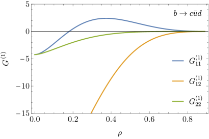
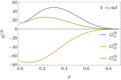
Figure 5: The NLO (left) and NNLO (right) corrections to different combinations of Wilson coefficients for $b\to c\bar{u}d$ as defined in Eq. (26) as functions of $\rho=m_{c}/m_{b}$ for $\mu_{b}=m_{b}$.

We can now turn to the prediction for the total rate $\Gamma^{cdu}$. We have to combine our results for the interference terms up to NNLO and the perturbative expansion of the Wilson coefficients at the low scale $\mu_{b}$ obtained with RGE at NNLO. The matching conditions for $C_{1}$ and $C_{2}$ in the historical basis can be obtained starting from those in the CMM basis [68] and then performing a basis transformation (see Appendix A.2, in particular Eq. (127)). The explicit expressions in the historical basis with anticommuting $\gamma_{5}$ read [34]:

$$C_{1}(\mu_{W}) =\frac{\alpha_{s}}{4\pi}\left(\frac{11}{2}+3L\right)$$

$$+\left(\frac{\alpha_{s}}{4\pi}\right)^{2}\left[\frac{64385}{3312}+\frac{17\pi^{2}}{6}-\frac{5}{9}n_{f}+\frac{415}{12}L+\frac{17}{2}L^{2}-\frac{1}{2}T\left(\frac{m_{t}^{2}}{M_{W}^{2}}\right)\right]+O(\alpha_{s}^{3}),$$

$$C_{2}(\mu_{W}) =1-\frac{\alpha_{s}}{4\pi}\left(\frac{11}{6}+L\right)$$

$$+\left(\frac{\alpha_{s}}{4\pi}\right)^{2}\left[-\frac{3894253}{49680}+\frac{7\pi^{2}}{18}-\frac{55}{36}L+\frac{7}{6}L^{2}+\frac{5}{27}n_{f}+\frac{1}{6}T\left(\frac{m_{t}^{2}}{M_{W}^{2}}\right)\right]+O(\alpha_{s}^{3}),$$ (38)

where $L=\log(\mu_{W}^{2}/M_{W}^{2})$. The function $T(x)$ parametrizes the top-quark mass effects. Its explicit expression can be retrieved from Eq. (19) in Ref. [68].

The solution of the RGE for the Wilson coefficients up to NNLO is well known and presented in Refs. [69, 34]. It requires the NNLO ADM in the historical basis, with the evanescent operator definition in Eq. (22). After performing a basis transformation of $\gamma^{(2)}$ from the CMM basis to the historical basis we obtain:

$$\hat{\gamma}^{(2)}=\begin{pmatrix}\frac{1340209}{460}-n_{f}\left(\frac{1190291}{6210}-\frac{80\zeta_{3}}{3}\right)+\frac{130}{81}n_{f}^{2}&\frac{401635}{276}-672\zeta_{3}-n_{f}\left(\frac{16657}{414}+80\zeta_{3}\right)-\frac{130}{27}n_{f}^{2}\\[10.0pt] \frac{401635}{276}-672\zeta_{3}-n_{f}\left(\frac{16657}{414}+80\zeta_{3}\right)-\frac{130}{27}n_{f}^{2}&\frac{1340209}{460}-n_{f}\left(\frac{1190291}{6210}-\frac{80\zeta_{3}}{3}\right)+\frac{130}{81}n_{f}^{2}\end{pmatrix},$$ (39)

With the matching conditions and the ADM up to NNLO, we can calculate the values of the Wilson coefficients at the low-energy scale $\mu_{b}\sim m_{b}$

$$C_{i}(\mu_{b})=C_{i}^{(0)}(\mu_{b})+\frac{\alpha_{s}(\mu_{b})}{4\pi}C_{i}^{(1)}(\mu_{b})+\left(\frac{\alpha_{s}(\mu_{b})}{4\pi}\right)^{2}C_{i}^{(2)}(\mu_{b})+O(\alpha_{s}^{3}),$$ (40)

which is appropriate for studying nonleptonic decay. We report in Tab. 1 the values for the Wilson coefficients at the reference scale $\mu_{b}=4.7$ GeV and matching scale $\mu_{W}=M_{W}$. For the numerical evaluation of $\alpha_{s}(\mu_{b})$ we use the five-loop RGE implemented in RunDec [70, 71] with $\alpha_{s}(M_{Z})=0.1179$.

	$i=1$	$i=2$
$C^{(0)}_{i}(\mu_{b})$	$-$0.2511	1.109
$C^{(1)}_{i}(\mu_{b})$	4.382	$-$2.016
$C^{(2)}_{i}(\mu_{b})$	36.63	$-$82.19

Table 1: Values of the Wilson coefficients $C_{1}(\mu_{b})$ and $C_{2}(\mu_{b})$ in the historical basis at LO, NLO and NNLO at the scale $\mu_{b}=4.7$ GeV. The matching scale is $\mu_{W}=M_{W}$.

After inserting the values for $C_{1}(\mu_{b})$ and $C_{2}(\mu_{b})$ into Eq. (26) and re-expanding it in series of $\alpha_{s}$ we obtain the perturbative expansion for the branching ratio in the on-shell scheme

$$\Gamma^{cdu} =\Gamma_{0}\left[1.89907+1.77538\frac{\alpha_{s}}{\pi}+14.1081\left(\frac{\alpha_{s}}{\pi}\right)^{2}\right],$$ (41)

with $\alpha_{s}=\alpha_{s}^{(5)}(m_{b})$, $m_{b}^{\mathrm{OS}}=4.7$ GeV and $m_{c}^{\mathrm{OS}}=1.3$ GeV. As a cross check, we repeated the calculation of the interference terms, the ADM and the Wilson coefficients at NNLO without specifying the numerical value for $A_{2}$ in Eq. (22) and (23). We explicitly verified that $A_{2}$ drops out in Eq. (41), so that the rate is independent on the scheme adopted for the evanescent operators. This represent a strong validation of our computational setup.

The dependence of the rate on the renormalization scale is presented in Fig. 6. In the plot we vary the scale $\mu_{b}$ associated to the strong coupling constant and the Wilson coefficients from $1\,\mathrm{GeV}<\mu_{b}<10\,\mathrm{GeV}$. We estimate the theoretical uncertainty by determining maximum and minimum for $\mu_{b}\in\{m_{b}/2,2m_{b}\}$ and dividing the result by two. We observe that the scale uncertainty is significantly reduced once higher order QCD corrections are included. Whereas at leading order the scale variation between $m_{b}/2$ and $2m_{b}$ yields a relative uncertainty of about 7%, which reduces to 6.3% at NLO, the inclusion of the NNLO corrections further reduce the scale uncertainty to 3.5% relative to the central value at $\mu_{b}=m_{b}$. At the central scale $\mu_{b}=m_{b}$ the $O(\alpha_{s})$ corrections are about 6.5% of the LO result and the $O(\alpha_{s}^{2})$ corrections are less than 3.5% of the prediction at NLO. Note that close to $\mu_{b}=m_{b}/2$ the NNLO corrections vanish.

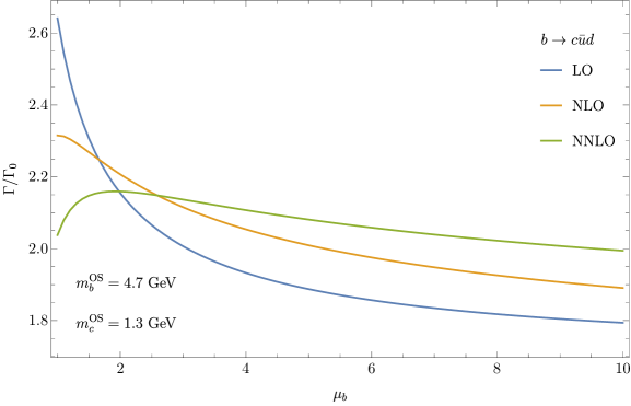
Figure 6: The dependence of the rate for $b\to c\bar{u}d$ on the renormalization scale $\mu_{b}\sim m_{b}$ at LO, NLO and NNLO in the on-shell scheme.

4.2 Massless contribution and secondary charm pair production

From the expressions for the $b\to c\bar{u}d$ decay, it is possible to take the limit $\rho\to 0$ and obtain the decay rate for $b\to u\bar{u}d$. We then add the $U_{c}$ contribution arising at $O(\alpha_{s}^{2})$ from the insertion of a closed charm loop into the gluon propagators (see for instance the diagram in Fig. 1(i). After inserting the values for $C_{1}$ and $C_{2}$, we obtain the perturbative expansion for the branching ratio in the massless limit:

$$\Gamma^{udu} =\Gamma_{0}\left[3.31981+0.597456\frac{\alpha_{s}}{\pi}+{\left(-25.645+0.254978_{U_{c}}\right)}\left(\frac{\alpha_{s}}{\pi}\right)^{2}\right],$$ (42)

where the last term arises from the $U_{c}$ contribution and depends on the ratio between the bottom and the charm mass. We use $m_{b}^{\mathrm{OS}}=4.7$ GeV and $m_{c}^{\mathrm{OS}}=1.3$ GeV. The dependence of the rate on the renormalization scale $\mu_{b}$ for the massless decay $b\to u\bar{u}d$ is presented in Fig. 7. We observe also here that for $m_{b}/2<\mu_{b}<2m_{b}$ the scale uncertainty is reduced from a relative 7% at LO, to 5% at NLO, to less than 1.3% after incorporating the NNLO corrections. At the central scale the NLO corrections are positive and amount to about 2% whereas the NNLO corrections are approximately twice as big and negative. However, close to $\mu_{b}=2m_{b}$ the NNLO corrections vanish.

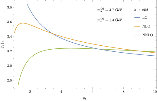
Figure 7: The dependence of the rate for $b\to u\bar{u}d$ on the renormalization scale $\mu_{b}\sim m_{b}$ at LO, NLO and NNLO in the on-shell scheme.

4.3 Two massive charm quarks: $b\to c\bar{c}s$

Also for the channel with two massive charm quarks in the final state we obtain analytic results at LO and NLO. For convenience we present in the following expansions around $\rho=0$. At LO we obtain

$$G_{11}^{(0)} =G_{22}^{(0)}=\frac{3}{2}G_{12}^{(0)}$$

$$=\frac{3(1-x^{2})\left(x^{12}-8x^{10}-43x^{8}-80x^{6}-43x^{4}-8x^{2}+1\right)}{\left(x^{2}+1\right)^{7}}$$

$$-\frac{144\left(x^{2}-x+1\right)\left(x^{2}+x+1\right)\left(x^{4}+3x^{2}+1\right)x^{4}\log(x)}{\left(x^{2}+1\right)^{8}}$$

$$=3\Big{(}1-16\rho^{2}+24\rho^{4}-32\rho^{6}+2\rho^{8}+32\rho^{10}+\left(-48\rho^{4}+48\rho^{8}\right)H_{0}(\rho)\Big{)}+\mathcal{O}\left(\rho^{12}\right)\,.$$ (43)

The analytic expressions for $b\to c\bar{c}s$ at NLO are rather lengthy and we report them only in the ancillary files attached to this paper [72, 73]. In the following we provide only the first few terms in an expansion around $\rho=0$.

$$G_{11}^{(1)} =\frac{31}{2}-2\pi^{2}-\left(320-32\pi^{2}+192l_{\rho}\right)\rho^{2}+\left[-276+64\pi^{2}+\left(336+64\pi^{2}\right)l_{\rho}-576l_{\rho}^{2}\right]\rho^{4}$$

$$+\left(-\frac{1552}{3}+\frac{160\pi^{2}}{3}-\frac{3200l_{\rho}}{3}-128l_{\rho}^{2}\right)\rho^{6}+\left[-\frac{7}{2}-108\pi^{2}+288\zeta(3)\right.$$

$$\left.+\left(\frac{88}{3}-64\pi^{2}\right)l_{\rho}+1264l_{\rho}^{2}\right]\rho^{8}+O(\rho^{9}),$$ (44)

$$G_{22}^{(1)} =\frac{31}{2}-2\pi^{2}+\left(-320+16\pi^{2}-192l_{\rho}\right)\rho^{2}+64\pi^{2}\rho^{3}+\left[-636-576l_{\rho}^{2}+16\pi^{2}\right.$$

$$\left.+l_{\rho}\left(528+32\pi^{2}\right)\right]\rho^{4}+\left(\frac{2696}{9}-\frac{16\pi^{2}}{3}-\frac{5312l_{\rho}}{3}-64l_{\rho}^{2}\right)\rho^{6}-64\pi^{2}\rho^{7}$$

$$+\left[-\frac{14236}{75}-68\pi^{2}-288\zeta(3)+1440l_{\rho}^{2}+l_{\rho}\left(-\frac{628}{5}+32\pi^{2}\right)\right]\rho^{8}+O(\rho^{9}),$$ (45)

$$G_{12}^{(1)} =-17-\frac{4\pi^{2}}{3}+\left(336+16\pi^{2}-128l_{\rho}\right)\rho^{2}-\frac{128\pi^{2}}{3}\rho^{3}+\left[-328-384l_{\rho}^{2}+l_{\rho}\left(1120\right.\right.$$

$$\left.\left.+\frac{128\pi^{2}}{3}\right)\right]\rho^{4}+\frac{256\pi^{2}}{3}\rho^{5}+\left[\frac{6008}{27}+\frac{176\pi^{2}}{9}+192\zeta(3)+l_{\rho}\left(\frac{128}{9}-\frac{128\pi^{2}}{3}\right)+64l_{\rho}^{2}\right]\rho^{6}$$

$$-128\pi^{2}\rho^{7}+\left[\frac{237341}{675}-\frac{104\pi^{2}}{9}+192\zeta(3)+l_{\rho}\left(-\frac{47152}{45}-\frac{128\pi^{2}}{3}\right)+\frac{1376l_{\rho}^{2}}{3}\right]\rho^{8}$$

$$+O(\rho^{9}).$$ (46)

One observes that the result at $\rho=0$ coincides with the massless limit in Eq. (34). For the NNLO result we obtain expansions around $\rho=0$, $\rho=1/5$ and $\rho=1/3$ using “expand and match” as described above. The expressions for the NNLO result expanded around $\rho=0$ read

$$G_{11}^{(2)} =13.4947-24.6740\rho+\left(-533.154-1251.35l_{\rho}+16.0000l_{\rho}^{2}\right)\rho^{2}$$

$$+\left(2998.33+210.551l_{\rho}\right)\rho^{3}+\left(116.662+10686.6l_{\rho}-628.278l_{\rho}^{2}+64.0000l_{\rho}^{3}\right)\rho^{4}$$

$$+\left(-2364.37+903.617l_{\rho}\right)\rho^{5}+\left(5409.89-6392.16l_{\rho}-5833.18l_{\rho}^{2}-507.259l_{\rho}^{3}\right)\rho^{6}$$

$$+\left(-135.120+3582.30l_{\rho}\right)\rho^{7}+\left(-2320.40-15254.6l_{\rho}+6047.29l_{\rho}^{2}+2654.91l_{\rho}^{3}\right)\rho^{8},$$ (47)

$$G_{22}^{(2)} =13.4947-24.6740\rho+\left(-3295.69-1883.01l_{\rho}+16.0000l_{\rho}^{2}\right)\rho^{2}$$

$$+\left(190.918-3842.56l_{\rho}\right)\rho^{3}+\left(4770.24+5244.57l_{\rho}-347.178l_{\rho}^{2}+64.0000l_{\rho}^{3}\right)\rho^{4}$$

$$+\left(1299.89-542.170l_{\rho}\right)\rho^{5}+\left(5832.60-7262.42l_{\rho}-10760.9l_{\rho}^{2}-271.407l_{\rho}^{3}\right)\rho^{6}$$

$$+\left(1667.93+1806.31l_{\rho}\right)\rho^{7}+\left(-30465.4-19154.5l_{\rho}+9435.28l_{\rho}^{2}+4491.90l_{\rho}^{3}\right)\rho^{8},$$ (48)

$$G_{12}^{(2)} =-72.8419-16.4493\rho+\left(3160.66+1152.54l_{\rho}+10.6666l_{\rho}^{2}\right)\rho^{2}$$

$$+\left(3980.72+2702.07l_{\rho}\right)\rho^{3}+\left(-5915.68+8133.91l_{\rho}+3393.24l_{\rho}^{2}+42.6666l_{\rho}^{3}\right)\rho^{4}$$

$$+\left(-8194.22+5070.78l_{\rho}\right)\rho^{5}+\left(18013.7+3710.59l_{\rho}+1222.25l_{\rho}^{2}+278.518l_{\rho}^{3}\right)\rho^{6}$$

$$+\left(184.414+7746.34l_{\rho}\right)\rho^{7}+\left(7997.58+2111.25l_{\rho}-9970.14l_{\rho}^{2}-773.168l_{\rho}^{3}\right)\rho^{8}.$$ (49)

In Fig. 8 the results for $G_{ij}^{(1)}$ and $G_{ij}^{(2)}$ are shown for $\rho\in[0,0.5]$.

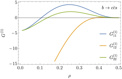
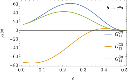
Figure 8: The NLO (left) and NNLO (right) corrections to different combinations of Wilson coefficients for $b\to c\bar{c}s$ as defined in Eq. (26) as functions of $\rho=m_{c}/m_{b}$ for $\mu_{b}=m_{b}$.

Evaluating the renormalized amplitude for $\mu_{b}=m_{b}^{\mathrm{OS}}$ we obtain the following numerical values for the decay width

$$\Gamma^{csc} =\Gamma_{0}\left[0.86706+3.15768\frac{\alpha_{s}}{\pi}+37.3426\left(\frac{\alpha_{s}}{\pi}\right)^{2}\right],$$ (50)

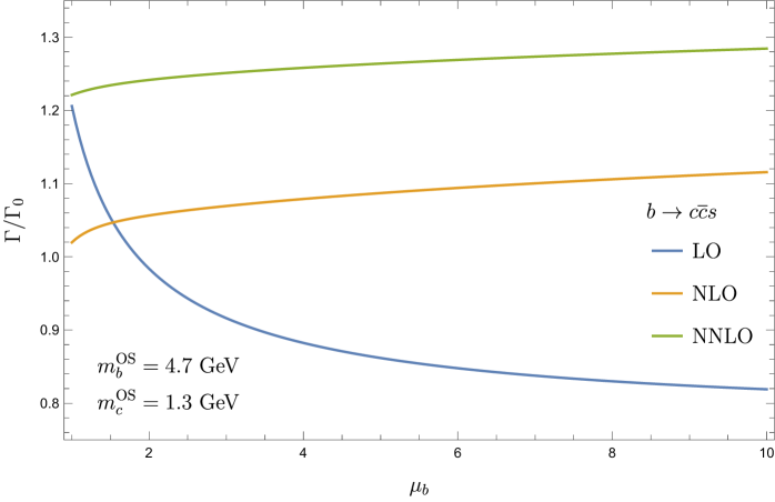
Figure 9: The dependence of the rate for $b\to c\bar{c}s$ on the renormalization scale $\mu_{b}\sim m_{b}$ at LO, NLO and NNLO in the on-shell scheme.

In Fig. 9 we show the dependence on the renormalization scale $\mu_{b}$. Already at NLO we observe a quite flat behaviour with a scale variation below 2.5%. It gets further reduced to about 1.5% at NNLO. As observed already in [74, 20, 24], the $O(\alpha_{s})$ corrections are rather large, about 25% of the LO prediction at $\mu_{b}=m_{b}$, and similarly the $O(\alpha_{s}^{2})$ corrections are 16% of the NLO prediction. Note that there is no overlap of the uncertainty band in the considered range of $\mu_{b}$. The NLO and NNLO prediction would differ by more than 5 sigma if the theoretical uncertainty is entirely based on the scale variation. A more conservative approach for the $b\to c\bar{c}s$ channel would be to take as uncertainty of the NNLO prediction half of the $O(\alpha_{s}^{2})$ corrections, which amounts to about 8%.

4.4 The CKM suppressed channel $b\to u\bar{c}s$

For the LO contribution we obtain the same result as in the $b\rightarrow c\bar{u}d$ decay channel in Eq. (28). Starting from NLO, the results differ from the $b\rightarrow c\bar{u}d$ case. We obtain

$$G_{11}^{(1)} =\frac{31}{2}-\frac{554}{3}\rho^{2}+\frac{554}{3}\rho^{6}-\frac{31}{2}\rho^{8}+\pi^{2}\left(-2+16\rho^{2}+48\rho^{4}-\frac{16}{3}\rho^{6}+\frac{2}{3}\rho^{8}+32\rho^{4}H_{0}(\rho)\right)$$

$$+\left(-\frac{62}{3}+\frac{640}{3}\rho^{2}-\frac{640}{3}\rho^{6}+\frac{62}{3}\rho^{8}\right)H_{-1}(\rho)+\left(-288\rho^{4}-64\rho^{6}+8\rho^{8}\right)\left(H_{0}(\rho)\right)^{2}$$

$$+\left(-96\rho^{2}-120\rho^{4}+\frac{992}{3}\rho^{6}-\frac{124}{3}\rho^{8}\right)H_{0}(\rho)+\left(\frac{62}{3}-\frac{640}{3}\rho^{2}+\frac{640}{3}\rho^{6}-\frac{62}{3}\rho^{8}\right)H_{1}(\rho)$$

$$+\left(8-64\rho^{2}-576\rho^{4}-64\rho^{6}+8\rho^{8}\right)\left[H_{0,1}(\rho)-H_{0,-1}(\rho)\right],$$ (51)

$$G_{22}^{(1)} =G_{11}^{(1)},$$ (52)

$$G_{12}^{(1)} =-17+\frac{932}{9}\rho^{2}-\frac{932}{9}\rho^{6}+17\rho^{8}+\left(-\frac{224}{3}\rho^{2}+\frac{2048}{3}\rho^{4}+\frac{4384}{9}\rho^{6}-\frac{344}{9}\rho^{8}\right)H_{0}(\rho)$$

$$+\pi^{2}\left(-\frac{4}{3}+\frac{80}{3}\rho^{2}-\frac{256}{3}\rho^{3}+96\rho^{4}-\frac{256}{3}\rho^{5}-\frac{16}{9}\rho^{6}+\frac{20}{9}\rho^{8}+\frac{128}{3}\rho^{4}H_{0}(\rho)\right)$$

$$+\left(-\frac{100}{9}+\frac{1952}{9}\rho^{2}-\frac{1952}{9}\rho^{6}+\frac{100}{9}\rho^{8}+\left(-\frac{32}{3}-\frac{128}{3}\rho^{2}-\frac{1024}{3}\rho^{3}-576\rho^{4}\right.\right.$$

$$\left.\left.-\frac{1024}{3}\rho^{5}-\frac{128}{3}\rho^{6}-\frac{32}{3}\rho^{8}\right)H_{0}(\rho)\right)H_{-1}(\rho)+\left(-192\rho^{4}-64\rho^{6}+16\rho^{8}\right)\left(H_{0}(\rho)\right)^{2}$$

$$+\left(\frac{100}{9}-\frac{1952}{9}\rho^{2}+\frac{1952}{9}\rho^{6}-\frac{100}{9}\rho^{8}+\left(\frac{32}{3}+\frac{128}{3}\rho^{2}-\frac{1024}{3}\rho^{3}+576\rho^{4}\right.\right.$$

$$\left.\left.-\frac{1024}{3}\rho^{5}+\frac{128}{3}\rho^{6}+\frac{32}{3}\rho^{8}\right)H_{0}(\rho)\right)H_{1}(\rho)$$

$$+\left(\frac{16}{3}+\frac{448}{3}\rho^{2}+\frac{1024}{3}\rho^{3}+1152\rho^{4}+\frac{1024}{3}\rho^{5}+\frac{448}{3}\rho^{6}+\frac{16}{3}\rho^{8}\right)H_{0,-1}(\rho)$$

$$+\left(-\frac{16}{3}-\frac{448}{3}\rho^{2}+\frac{1024}{3}\rho^{3}-1152\rho^{4}+\frac{1024}{3}\rho^{5}-\frac{448}{3}\rho^{6}-\frac{16}{3}\rho^{8}\right)H_{0,1}(\rho).$$ (53)

One observes, that the coefficients $G_{22}^{(1)}$ and $G_{11}^{(1)}$ are the same in this decay channel. The NNLO results expanded around $\rho=0$ read

$$G_{11}^{(2)} =13.4947-24.6740\rho+\left(-552.675-591.011l_{\rho}-8.00000l_{\rho}^{2}\right)\rho^{2}$$

$$+\left(3314.34+210.551l_{\rho}\right)\rho^{3}+\left(-1000.88+5447.49l_{\rho}-505.906l_{\rho}^{2}-64.0000l_{\rho}^{3}\right)\rho^{4}$$

$$+\left(387.348+328.986l_{\rho}\right)\rho^{5}+\left(-2248.02+240.114l_{\rho}+1066.01l_{\rho}^{2}-264.296l_{\rho}^{3}\right)\rho^{6}$$

$$+\left(-159.907+306.177l_{\rho}\right)\rho^{7}+\left(306.693-508.164l_{\rho}+133.563l_{\rho}^{2}-66.3703l_{\rho}^{3}\right)\rho^{8},$$ (54)

$$G_{22}^{(2)} =G_{11}^{(2)},$$ (55)

$$G_{12}^{(2)} =-72.8419-16.4493\rho+\left(3424.97+1112.31l_{\rho}+5.33333l_{\rho}^{2}+\right)\rho^{2}$$

$$+\left(7782.51+5404.15l_{\rho}\right)\rho^{3}+\left(-72.4205+15986.63l_{\rho}+727.426l_{\rho}^{2}-42.6666l_{\rho}^{3}\right)\rho^{4}$$

$$+\left(-2108.79+9301.11l_{\rho}\right)\rho^{5}+\left(-8020.41+2479.56l_{\rho}+1176.61l_{\rho}^{2}-311.703l_{\rho}^{3}\right)\rho^{6}$$

$$+\left(629.490+1924.62l_{\rho}\right)\rho^{7}+\left(-1269.71-34.1428l_{\rho}-26.6329l_{\rho}^{2}+81.3497l_{\rho}^{3}\right)\rho^{8}.$$ (56)

The limit for $\rho=0$ coincides with the result obtained from $b\to c\bar{u}d$ and $b\to c\bar{c}s$ calculations.

At the central scale we obtain the following expansion of the decay rate

$$\Gamma^{ucs} =\Gamma_{0}\left[1.88907+4.39458\frac{\alpha_{s}}{\pi}{-33.5725}\left(\frac{\alpha_{s}}{\pi}\right)^{2}\right]\,.$$ (57)

The dependence on $\mu_{b}$ in Fig. 10 shows a slight reduction from 7.3% to 6.1% when going from NLO to NNLO.

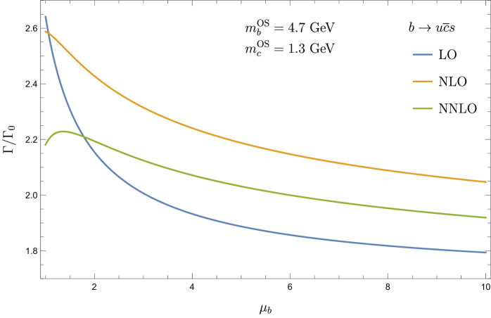
Figure 10: The dependence of the rate for $b\to u\bar{c}s$ on the renormalization scale $\mu_{b}\sim m_{b}^{\mathrm{OS}}$ at LO, NLO and NNLO in the on-shell scheme.

4.5 Combined decay channels

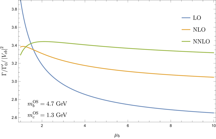
Figure 11: All contributing decay channels combined.

The total decay width at partonic level is obtained from the incoherent sum of all individual channels discussed before. In particular, we include the contributions from $b\to c\bar{u}d$, $b\to c\bar{u}s$, $b\to c\bar{c}d$, $b\to c\bar{c}s$, $b\to u\bar{c}d$, $b\to u\bar{c}s$, $b\to u\bar{u}d$ and $b\to u\bar{u}s$. The width is in a first approximation given by the sum of the two channel $b\to c\bar{u}d$ and $b\to c\bar{c}s$ since $|V_{ud}|\simeq|V_{cs}|\simeq 1$. Other channels are CKM suppressed and lead to additional small corrections. We obtain for $\mu_{b}=m_{b}^{\mathrm{OS}}$ the numerical values

$$\Gamma\Big{|}_{\mathrm{all\,nonlep,\,partonic}} =\Gamma^{\prime}_{0}\left[0.00474256+0.00839798\frac{\alpha_{s}}{\pi}+0.0859442\left(\frac{\alpha_{s}}{\pi}\right)^{2}\right],$$

$$=\Gamma_{0}^{\prime}|V_{cb}|^{2}\left[2.79101+4.93227\frac{\alpha_{s}}{\pi}+51.1826\left(\frac{\alpha_{s}}{\pi}\right)^{2}\right],$$ (58)

where we define $\Gamma^{\prime}_{0}=G_{F}^{2}(m_{b}^{\mathrm{OS}})^{5}/(192\pi^{3})$ as the normalization of the decay width. We use the following numerical input for the CKM matrix elements [75]:

$$|V_{ud}| =0.97435\pm 0.00016, |V_{us}| =0.22501\pm 0.00068, |V_{ub}| =(3.732^{+0.090}_{-0.085})\times 10^{-3},$$

$$|V_{cd}| =0.22487\pm 0.00068, |V_{cs}| =0.97349\pm 0.00016, |V_{cb}| =(4.183^{+0.079}_{-0.069})\times 10^{-2}.$$ (59)

The decay $b\to c\bar{u}d$ gives about 59% of the total sum in Eq. (58), while $b\to c\bar{c}s$ contribute about 36%. The remaining 5% is given by all other CKM suppressed modes. We observe that the NNLO corrections come with the same sign as the NLO corrections in the relevant region of the renormalization scale $\mu_{b}$. Using RunDec, we obtain $\alpha_{s}(\mu_{b}=4.7\,\mathrm{GeV})=0.2166$ and find that the term of $O(\alpha_{s}^{2})$ is roughly 50-60% of the one at $O(\alpha_{s})$ for $\mu_{b}=m_{b}^{\mathrm{OS}}$. The scale uncertainty reduces from a relative 3.5% at NLO to 1.7% at NNLO. From Fig. 11 we observe that the NNLO curve is flatter than the LO and NLO ones, however also in the sum of all channels, the predictions at NLO and NNLO differs by about 2$\sim$sigma, once the theoretical uncertainties are evaluated from the scale variation between $m_{b}/2<\mu_{b}<2m_{b}$.

5 Conclusions

In this paper we provide an important contribution to the hadronic $B$ meson decay rate. We compute NNLO corrections to all relevant partonic channels taking into account finite bottom and charm quark masses. In the effective theory we take into account the current-current operators together with the relevant evanescent operators such that it is possible to use anti-commuting $\gamma_{5}$ for our calculation. For the computation of the Feynman integrals we use the “expand and match” method. It uses the differential equations for the master integrals in order to construct analytic expansions around properly chosen values for $m_{c}/m_{b}$ with high-precision numerical coefficients. This leads to compact expressions which are can be evaluated numerically in a straightforward way.

We perform a preliminary numerical study of the impact of the NNLO corrections in the various channels considered using pole scheme for the quark masses. Overall we find that the theoretical uncertainties stemming from the scale variation is reduced by more than a factor of three for $b\to c\bar{u}d$. The reduction for the channel $b\to c\bar{c}s$ is about a factor of two, however we notice that the NLO and NNLO predictions do not overlap withing the assigned uncertainties, due to large corrections arising at order $\alpha_{s}$ and $\alpha_{s}^{2}$.

Our analytic results for all decay modes are provided in electronic form and can be retrieved from the repository [72, 73]. An update of the lifetime prediction of $B$ meson is ongoing where we include the novel NNLO corrections presented in this paper and combine them with updated prediction for the power suppressed terms and quark masses [33]. Our results can also be easily applied to decays of $D$ mesons.

Appendix A Operator mixing

A.1 Calculation of renormalization constants

For our calculation we need the renormalization constants for the mixing of the effective operators $O_{1}$ and $O_{2}$ in the historical basis up to two loops. The results can be found in Refs. [69, 76, 77, 35], however, not in the form suitable for our calculation, which is performed keeping the full dependence on $N_{C}$. For this reason we decided to repeat the calculation in our setup, which is also a good check on the correct implementation of the effective operators. Note that higher-order results for the renormalization constants and anomalous dimensions are available in the CMM basis [78, 79, 34, 80, 81]. Furthermore, transformation rules allow to convert the results from the historical to the CMM basis and vice versa [35, 82, 34].

In the following we briefly describe the calculation of the renormalization constants for the physical and evanescent operators appearing in our calculation. We consider the matrix element $A_{\mathrm{eff}}=\sum_{i}C_{i}\bra{cd}O_{i}\ket{bu}$ of the effective operators with four external quarks (e.g. $bu\to cd$). At higher order in $\alpha_{s}$, $A_{\mathrm{eff}}$ contains ultraviolet (UV) poles after renormalization of the masses, the strong coupling constant and the quark wave functions. They must be subtracted via the renormalization of the Wilson coefficients,

$$C_{i,B}=Z_{ji}C_{j}(\mu_{b}),$$ (60)

where $C_{i,B}$ and $C_{i}(\mu_{b})$ denote the bare and renormalized Wilson coefficients, respectively. Schematically, the matrix element of the operators is given by

$$A_{\mathrm{eff}}=C_{j}(\mu_{b})Z_{ji}\langle Z(O_{i})\rangle_{R},$$ (61)

where $\langle Z(O_{i})\rangle_{R}$ describes the expectation value of the operator $O_{i}$ including wave function, quark mass and coupling constant renormalization. The renormalization constants $Z_{ij}$ can be obtained order by order in $\alpha_{s}$ by requiring that Eq. (61) is free of UV poles.

The renormalization constants $Z_{ij}$ have the perturbative expansion

$$Z_{ij}=\delta_{ij}+\sum_{k=1}^{\infty}\left(\frac{\alpha_{s}}{4\pi}\right)^{k}Z_{ij}^{(k)},$$ (62)

where

$$Z_{ij}^{(k)}=\sum_{l=0}^{k}\frac{Z_{ij}^{(k,l)}}{\epsilon^{l}}.$$ (63)

We use the $\overline{\mathrm{MS}}$ renormalization scheme, which implies $l>0$. This is, however, not the case if $i$ is the coefficient of an evanescent operator, while $j$ corresponds to a physical one. In these cases, the renormalization constants include $\epsilon$-finite terms that ensure that the matrix elements of evanescent operators vanish in four dimensions (see Ref. [83, 84]).

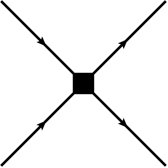
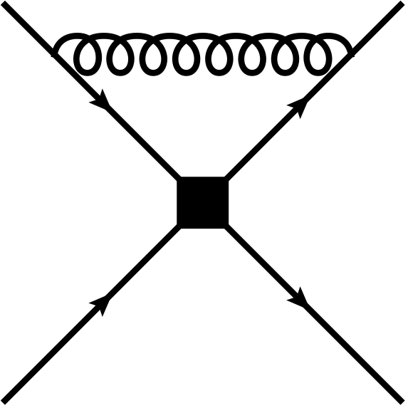
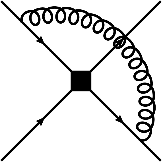
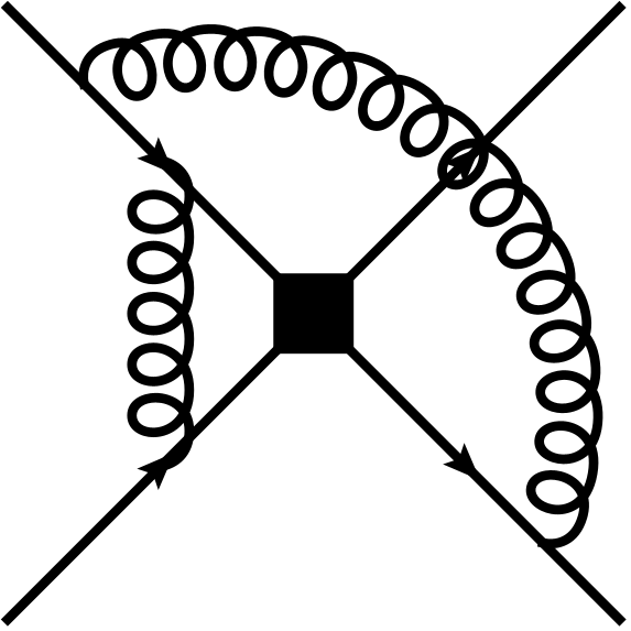
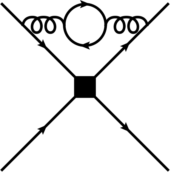
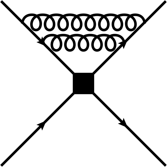
Figure 12: Sample Feynman diagrams with four external quark lines and the insertion of one of the effective operators at tree-level, one- and two-loop order. All the quarks are massive and the external momenta are set to zero. The square denotes the insertion of an effective four fermion operator.

For the calculation of the renormalization constants we consider operator matrix elements for $\{O_{1},O_{2},E_{1}^{(1)},E_{2}^{(1)},E_{1}^{(2)},E_{2}^{(2)}\}$ with four external quark lines up two-loop order, see Fig. 12 for some sample diagrams. Since these Feynman diagrams are logarithmically divergent and since we are only interested in the UV divergence, we are allowed to choose a convenient kinematic limit for their computation. In order to avoid infrared divergences, we assign to all quarks the same mass, keep the gluons and ghosts massless and set the external momenta to zero. This leads to one-scale vacuum integrals which are conveniently computed with the help of MATAD [85].

After the calculation of the loop integrals, the result contains terms with up to nine $\gamma$ matrices and different colour structures. We use the usual commutation relations and bring the products of $\gamma$ matrices in a form which allows us to identify the contributions from the physical and evanescent operators in Eqs. (3) and (22), respectively. For our calculation we need in addition higher order evanescent operators given by

$$E_{5}= \left(\bar{q}_{1}^{i}\gamma^{\mu_{1}\dots\mu_{7}}P_{L}b^{j}\right)\left(\bar{q}_{2}^{i}\gamma_{\mu_{1}\dots\mu_{7}}P_{L}q_{3}^{j}\right)-(4096-7680\epsilon)O_{1},$$

$$E_{6}= \left(\bar{q}_{1}^{i}\gamma^{\mu_{1}\dots\mu_{7}}P_{L}b^{i}\right)\left(\bar{q}_{2}^{j}\gamma_{\mu_{1}\dots\mu_{7}}P_{L}q_{3}^{j}\right)-(4096-7680\epsilon)O_{2},$$

$$E_{7}= \left(\bar{q}_{1}^{i}\gamma^{\mu_{1}\dots\mu_{9}}P_{L}b^{j}\right)\left(\bar{q}_{2}^{i}\gamma_{\mu_{1}\dots\mu_{9}}P_{L}q_{3}^{j}\right)-(65536-176128\epsilon)O_{1},$$

$$E_{8}= \left(\bar{q}_{1}^{i}\gamma^{\mu_{1}\dots\mu_{9}}P_{L}b^{i}\right)\left(\bar{q}_{2}^{j}\gamma_{\mu_{1}\dots\mu_{9}}P_{L}q_{3}^{j}\right)-(65536-176128\epsilon)O_{2}.$$ (64)

The $O(\epsilon)$ terms can be obtained following Ref. [86]; in the case of $E_{5}$ and $E_{6}$ they can also be found in Ref. [87].

Once the bare result is expressed as a linear combination of (bare) operator matrix elements, we perform the parameter renormalization (wave function, quark mass and strong coupling constant) in the $\overline{\rm MS}$ scheme and introduce the $Z_{ij}$ according to Eq. (61), where the unknown coefficients are obtained from the requirement that the renormalized operator matrix elements are finite.

Our results for the one-loop renormalization constants for the following set of physical and evanescent operators

$$\vec{Q}^{T} =(O_{1},O_{2}), \vec{E}^{T} =(E_{1}^{(1)},E_{2}^{(1)},E_{1}^{(2)},E_{2}^{(2)}),$$ (65)

are given by

$$Z^{(1,1)} =\left(\begin{array}[]{c c c c c c}-1&3&\frac{7}{12}&\frac{1}{4}&0&0\\[5.0pt] 3&-1&\frac{1}{2}&-\frac{1}{6}&0&0\\[5.0pt] 0&0&-\frac{59}{3}&-5&\frac{7}{12}&\frac{1}{4}\\[5.0pt] 0&0&-13&\frac{13}{3}&\frac{1}{2}&-\frac{1}{6}\\[5.0pt] 0&0&-\frac{1888}{3}&96&\frac{41}{3}&-9\\[5.0pt] 0&0&-288&\frac{1568}{3}&3&-\frac{67}{3}\end{array}\right),$$ (72)

$$Z^{(1,0)} =\left(\begin{array}[]{c c c c c c}0&0&0&0&0&0\\[5.0pt] 0&0&0&0&0&0\\[5.0pt] 16&-48&0&0&0&0\\[5.0pt] -24&-56&0&0&0&0\\[5.0pt] 512&-1536&0&0&0&0\\[5.0pt] -768&-1792&0&0&0&0\end{array}\right)\,,$$ (79)

and at two loops we have

$$Z^{(2,2)} =\left(\begin{array}[]{cccccc}\frac{21}{2}&-\frac{39}{2}&-\frac{91}{9}&-\frac{8}{3}&\frac{67}{288}&\frac{5}{96}\\[5.0pt] -\frac{39}{2}&\frac{21}{2}&-\frac{143}{24}&-\frac{17}{72}&\frac{5}{48}&\frac{11}{144}\\[5.0pt] 0&0&\frac{229}{2}&\frac{955}{6}&-\frac{35}{6}&-\frac{53}{6}\\[5.0pt] 0&0&\frac{227}{6}&-\frac{3}{2}&-\frac{55}{24}&-\frac{35}{24}\\[5.0pt] 0&0&\frac{13360}{9}&\frac{5200}{3}&-\frac{2273}{6}&\frac{907}{6}\\[5.0pt] 0&0&\frac{1424}{3}&-\frac{63248}{9}&-\frac{793}{6}&\frac{1675}{6}\end{array}\right)$$ (86)

$$+n_{f}\left(\begin{array}[]{cccccc}-\frac{1}{3}&1&\frac{7}{36}&\frac{1}{12}&0&0\\[5.0pt] 1&-\frac{1}{3}&\frac{1}{6}&-\frac{1}{18}&0&0\\[5.0pt] 0&0&-\frac{59}{9}&-\frac{5}{3}&\frac{7}{36}&\frac{1}{12}\\[5.0pt] 0&0&-\frac{13}{3}&\frac{13}{9}&\frac{1}{6}&-\frac{1}{18}\\[5.0pt] 0&0&-\frac{1888}{9}&32&\frac{41}{9}&-3\\[5.0pt] 0&0&-96&\frac{1568}{9}&1&-\frac{67}{9}\end{array}\right),$$ (93)

$$Z^{(2,1)} =\left(\begin{array}[]{cccccc}-\frac{23}{24}&-\frac{161}{8}&\frac{323}{36}&\frac{7}{12}&-\frac{1}{36}&-\frac{5}{48}\\[5.0pt] \frac{55}{8}&-\frac{239}{24}&\frac{51}{8}&\frac{115}{72}&-\frac{35}{384}&-\frac{77}{1152}\\[5.0pt] -212&252&-\frac{1279}{24}&-\frac{697}{8}&\frac{145}{24}&\frac{49}{24}\\[5.0pt] 96&256&-\frac{1963}{24}&\frac{2753}{24}&\frac{89}{12}&-\frac{1}{12}\\[5.0pt] -3968&11904&\frac{32488}{9}&1704&\frac{9257}{24}&-\frac{2817}{8}\\[5.0pt] 4992&16768&-\frac{12748}{3}&\frac{101644}{9}&\frac{6985}{24}&\frac{2117}{24}\end{array}\right)$$ (100)

$$+n_{f}\left(\begin{array}[]{cccccc}-\frac{1}{18}&\frac{1}{6}&-\frac{7}{216}&-\frac{1}{72}&0&0\\[5.0pt] \frac{1}{6}&-\frac{1}{18}&-\frac{1}{36}&\frac{1}{108}&0&0\\[5.0pt] \frac{16}{3}&-16&\frac{353}{54}&-\frac{1}{18}&-\frac{7}{216}&-\frac{1}{72}\\[5.0pt] -8&-\frac{56}{3}&\frac{67}{18}&-\frac{259}{54}&-\frac{1}{36}&\frac{1}{108}\\[5.0pt] \frac{512}{3}&-512&\frac{4280}{27}&-\frac{40}{3}&\frac{427}{54}&-\frac{3}{2}\\[5.0pt] -256&-\frac{1792}{3}&80&-\frac{3280}{27}&\frac{7}{2}&-\frac{383}{54}\end{array}\right),$$ (107)

$$Z^{(2,0)} =\left(\begin{array}[]{cccccc}0&0&0&0&0&0\\ 0&0&0&0&0&0\\ \frac{202796}{115}-\frac{50488n_{f}}{1035}&\frac{1037132}{115}-\frac{25544n_{f}}{345}&0&0&0&0\\[5.0pt] -\frac{15148n_{f}}{345}-\frac{39856}{115}&\frac{46028n_{f}}{1035}+\frac{39904}{23}&0&0&0&0\\[5.0pt] \frac{4098848}{1035}-\frac{1561184n_{f}}{1035}&\frac{1154912n_{f}}{345}-\frac{1011808}{15}&0&0&0&0\\[5.0pt] \frac{56192n_{f}}{69}-\frac{34695184}{345}&\frac{6995584n_{f}}{1035}-\frac{282282736}{1035}&0&0&0&0\end{array}\right).$$ (114)

We have performed the calculation for general SU($N_{c}$) gauge groups; the corresponding analytic expressions can be found in the supplementary material to this paper [72, 73]. For simplicity we present the results for $N_{c}=3$ and only keep the the number of active flavours $n_{f}$ in the analytic expressions. In the numerical analysis we use $n_{f}=5$.

At first sight it looks strange that with our approach also the finite terms in $Z^{(1,0)}$ and $Z^{(2,0)}$ can be determined. Note, however, that they originate from divergent part of loop integrals multiplied by factor of $\epsilon$ from the Dirac algebra in the numerator of the Feynman diagrams. Our calculation has been performed for general QCD gauge parameter which drops out in the final results for the renormalization constants. Furthermore, after converting the renormalization constants to the anomalous dimension matrix, we agree with the results in Eq. (57) of Ref. [35].

Our setup is validated also by reproducing the well known results in the CMM basis. For the calculation of the $Z_{ij}$ in the CMM basis, we use the physical operators from Eq. (4). The evanescent operators are given by

$$E_{1}^{\prime} =\left(\bar{q}_{1}\gamma^{\mu_{1}\mu_{2}\mu_{3}}T^{a}P_{L}b\right)\left(\bar{q}_{2}\gamma_{\mu_{1}\mu_{2}\mu_{3}}T^{a}P_{L}q_{3}\right)-16O_{1}^{\prime},$$

$$E_{2}^{\prime} =\left(\bar{q}_{1}\gamma^{\mu_{1}\mu_{2}\mu_{3}}P_{L}b\right)\left(\bar{q}_{2}\gamma_{\mu_{1}\mu_{2}\mu_{3}}P_{L}q_{3}\right)-16O_{2}^{\prime},$$

$$E_{3}^{\prime} =\left(\bar{q}_{1}\gamma^{\mu_{1}\dots\mu_{5}}T^{a}P_{L}b\right)\left(\bar{q}_{2}\gamma_{\mu_{1}\dots\mu_{5}}T^{a}P_{L}q_{3}\right)-256O_{1}^{\prime}-20E_{1}^{\prime},$$

$$E_{4}^{\prime} =\left(\bar{q}_{1}\gamma^{\mu_{1}\dots\mu_{5}}P_{L}b\right)\left(\bar{q}_{2}\gamma_{\mu_{1}\dots\mu_{5}}P_{L}q_{3}\right)-256O_{2}^{\prime}-20E_{2}^{\prime}\,,$$

$$E_{5}^{\prime} =\left(\bar{q}_{1}\gamma^{\mu_{1}\dots\mu_{7}}T^{a}P_{L}b\right)\left(\bar{q}_{2}\gamma_{\mu_{1}\dots\mu_{7}}T^{a}P_{L}q_{3}\right)-4096O_{1}^{\prime}-336E_{1}^{\prime},$$

$$E_{6}^{\prime} =\left(\bar{q}_{1}\gamma^{\mu_{1}\dots\mu_{7}}P_{L}b\right)\left(\bar{q}_{2}\gamma_{\mu_{1}\dots\mu_{7}}P_{L}q_{3}\right)-4096O_{2}^{\prime}-336E_{2}^{\prime},$$

$$E_{7}^{\prime} =\left(\bar{q}_{1}\gamma^{\mu_{1}\dots\mu_{9}}T^{a}P_{L}b\right)\left(\bar{q}_{2}\gamma_{\mu_{1}\dots\mu_{9}}T^{a}P_{L}q_{3}\right)-65536O_{1}^{\prime}-5440E_{1}^{\prime},$$

$$E_{8}^{\prime} =\left(\bar{q}_{1}\gamma^{\mu_{1}\dots\mu_{9}}P_{L}b\right)\left(\bar{q}_{2}\gamma_{\mu_{1}\dots\mu_{9}}P_{L}q_{3}\right)-65536O_{2}^{\prime}-5440E_{2}^{\prime}\,.$$ (115)

We were able to reproduce the results from Ref. [34]. Furthermore we use the formalism developed in Refs. [35, 82] and translate the renormalization constants from the CMM to the historical basis (see also next subsection), which confirms the results given in Eqs. (79) and (114).

A.2 Change of basis

In order to calculate the NNLO anomalous dimension in Eq. (39) in the historical basis fulfilling the condition (17) and to compare the renormalization constants with known results for the CMM basis in the literature, we have to perform a basis transformation. In the following we adopt the formalism developed in [35, 82, 87] to describe the basis change between the CMM basis and the historical basis. Let us denote by

$$\vec{Q}^{{}^{\prime}T} =(O_{1}^{\prime},O_{2}^{\prime}),$$

$$\vec{E}^{{}^{\prime}T} =(E_{1}^{\prime},E_{2}^{\prime},E_{3}^{\prime},E_{4}^{\prime}),$$ (116)

the physical and evanescent operators in the CMM basis. For physical operators, the basis change is a simple linear transformation

$$\vec{Q}=\hat{R}\vec{Q}^{\prime},$$ (117)

where in our case $\hat{R}$ is a $2\times 2$ matrix. For the evanescent operators, the transformation rule is

$$\vec{E}=\hat{M}\Big{[}\vec{E}^{\prime}+\epsilon\hat{U}\vec{Q}^{\prime}+\epsilon^{2}\hat{V}\vec{Q}^{\prime}\Big{]},$$ (118)

where the $n\times 2$ matrices $\hat{U}$ and $\hat{V}$ and the $n\times n$ matrix $\hat{M}$ parametrize the rotation of evanescent operators. The basis change for the operator set $(\vec{Q},\vec{E})$ is encoded by two $\epsilon$-dependent linear transformations,

$$\hat{A} =\begin{pmatrix}\hat{R}&0\\ 0&\hat{M}\end{pmatrix}, \hat{B} =\begin{pmatrix}1&0\\ \epsilon\hat{U}+\epsilon^{2}\hat{V}&1\end{pmatrix},$$ (119)

so that renormalization constants in the two bases are related by

$$\hat{Z}=(\hat{A}\hat{B})Z^{\prime}(\hat{B}^{-1}\hat{A}^{-1}).$$ (120)

The transformation matrices from the CMM basis to the historical basis with the evanescent operators defined in Eq. (22) and $A_{2}=-4$ are

$$\hat{R} =\begin{pmatrix}2&1/3\\ 0&1\end{pmatrix}, \hat{M} =\begin{pmatrix}2&\frac{1}{3}&0&0&0&0\\ 0&1&0&0&0&0\\ 40&\frac{20}{3}&2&\frac{1}{3}&0&0\\ 0&20&0&1&0&0\\ 672&112&0&0&2&\frac{1}{3}\\ 0&336&0&0&0&1\\ \end{pmatrix},$$

$$\hat{U} =\begin{pmatrix}4&0\\ 0&4\\ 144&0\\ 0&144\\ 6336&0\\ 0&6336\\ \end{pmatrix}, \hat{V} =\begin{pmatrix}4&0\\ 0&4\\[5.0pt] \frac{36736}{115}&-\frac{2304}{23}\\[5.0pt] 0&\frac{105856}{115}\\[5.0pt] -1344&0\\ 0&-1344\\ \end{pmatrix}.$$ (121)

By focusing on the various subblocks of the renormalization matrices,

$$\hat{Z}=\begin{pmatrix}\hat{Z}_{QQ}&\hat{Z}_{QE}\\ \hat{Z}_{EQ}&\hat{Z}_{EE}\end{pmatrix},$$ (122)

we can give the transformation rules at order $\alpha_{s}$

$$\hat{Z}_{QQ}^{(1,1)} =\hat{R}\hat{Z}^{{}^{\prime}(1,1)}_{QQ}\hat{R}^{-1}, \hat{Z}_{QE}^{(1,1)} =\hat{R}\hat{Z}^{{}^{\prime}(1,1)}_{QE}\hat{M}^{-1},$$

$$\hat{Z}_{EE}^{(1,1)} =\hat{M}\hat{Z}^{{}^{\prime}(1,1)}_{EE}\hat{M}^{-1}, \hat{Z}_{QQ}^{(1,0)} =-\hat{R}\hat{Z}_{QE}^{{}^{\prime}(1,1)}\hat{U}\hat{R}^{-1},$$

$$\hat{Z}_{EQ}^{(1,0)} =\hat{M}\Big{[}\hat{Z}^{{}^{\prime}(1,0)}_{EQ}+\hat{U}\hat{Z}_{QQ}^{{}^{\prime}(1,1)}-\hat{Z}_{EE}^{{}^{\prime}(1,1)}\hat{U}\Big{]}\hat{R}^{-1}.$$ (123)

At order $\alpha_{s}^{2}$ we have

$$\hat{Z}_{QQ}^{(2,2)} =\hat{R}\hat{Z}^{{}^{\prime}(2,2)}_{QQ}\hat{R}^{-1},$$

$$\hat{Z}_{QE}^{(2,2)} =\hat{R}\hat{Z}^{{}^{\prime}(2,2)}_{QE}\hat{M}^{-1},$$

$$\hat{Z}_{EE}^{(2,2)} =\hat{M}\hat{Z}^{{}^{\prime}(2,2)}_{EE}\hat{M}^{-1},$$

$$\hat{Z}_{QQ}^{(2,1)} =\hat{R}\Big{[}\hat{Z}^{{}^{\prime}(2,1)}_{QQ}-\hat{Z}^{{}^{\prime}(2,2)}_{QE}\hat{U}\Big{]}\hat{R}^{-1},$$

$$\hat{Z}_{QE}^{(2,1)} =\hat{R}\hat{Z}^{{}^{\prime}(2,1)}_{QE}\hat{M}^{-1},$$

$$\hat{Z}_{EE}^{(2,1)} =\hat{R}\Big{[}\hat{Z}^{{}^{\prime}(2,1)}_{EE}-\hat{U}\hat{Z}^{{}^{\prime}(2,2)}_{QE}\Big{]}\hat{M}^{-1},$$

$$\hat{Z}_{EQ}^{(2,1)} =\hat{M}\Big{[}\hat{Z}^{{}^{\prime}(2,1)}_{EQ}+\hat{U}\hat{Z}^{{}^{\prime}(2,2)}_{QQ}-\hat{Z}^{{}^{\prime}(2,2)}_{EE}\hat{U}\Big{]}\hat{R}^{-1},$$

$$\hat{Z}_{QQ}^{(2,0)} =\hat{R}\Big{[}-\hat{Z}^{{}^{\prime}(2,1)}_{QE}\hat{U}-\hat{Z}^{{}^{\prime}(2,2)}_{QE}\hat{V}+{\hat{Z}_{QE}^{{}^{\prime}(1,1)}}\hat{V}\hat{Z}_{QQ}^{{}^{\prime}(1,1)}\Big{]}\hat{R}^{-1}$$

$$\hat{Z}_{EQ}^{(2,0)} =\hat{M}\Big{[}\hat{Z}^{{}^{\prime}(2,0)}_{EQ}+\hat{U}\hat{Z}^{{}^{\prime}(2,1)}_{QQ}+\hat{V}\hat{Z}^{{}^{\prime}(2,2)}_{QQ}-\hat{Z}^{{}^{\prime}(2,1)}_{EE}\hat{U}-\hat{Z}^{{}^{\prime}(2,2)}_{EE}\hat{V}-\hat{U}\hat{Z}^{{}^{\prime}(2,2)}_{QE}\hat{U}\Big{]}\hat{R}^{-1}.$$ (124)

After rotating the CMM basis into the historical basis, the element $\hat{Z}^{(1,0)}_{QQ}$ and $\hat{Z}^{(2,0)}_{QQ}$ are different from zero and therefore they do not corresponds to an $\overline{\mathrm{MS}}$ renormalization scheme. Such finite contributions must be removed by a suitable change of scheme. For the renormalization constants this corresponds to the transformation

$$\hat{Z}_{\overline{\mathrm{MS}}}=\left[1-\frac{\alpha_{s}}{4\pi}\hat{r}_{1}-\left(\frac{\alpha_{s}}{4\pi}\right)^{2}(\hat{r}_{2}-\hat{r}_{1}^{2})\right]\hat{Z},$$ (125)

where for the subblock corresponding to the physical operators we obtain

$$(\hat{r}_{1})_{QQ} =\hat{Z}_{QQ}^{(1,0)}=\begin{pmatrix}-\frac{7}{3}&-1\\ -2&\frac{2}{3}\end{pmatrix},$$

$$(\hat{r}_{2})_{QQ} =\hat{Z}_{QQ}^{(2,0)}=\begin{pmatrix}-\frac{153257}{2070}-\frac{35}{54}n_{f}&-\frac{1763}{138}-\frac{5}{18}n_{f}\\[5.0pt] -\frac{6493}{276}-\frac{5}{9}n_{f}&-\frac{239239}{4140}+\frac{5}{27}n_{f}\end{pmatrix}.$$ (126)

The transformation rule for the Wilson coefficients is

$$\vec{C}(\mu_{b})=\vec{C}^{\prime}(\mu_{b})\hat{R}^{-1}\left[1+\frac{\alpha_{s}}{4\pi}(\hat{r}_{1})_{QQ}+\left(\frac{\alpha_{s}}{4\pi}\right)^{2}(\hat{r}_{2})_{QQ}\right],$$ (127)

while the ADMs transform in the following way:

$$\hat{\gamma}^{(0)} =\hat{R}\hat{\gamma}^{{}^{\prime}(0)}\hat{R}^{-1},$$

$$\hat{\gamma}^{(1)} =\hat{R}\hat{\gamma}^{{}^{\prime}(1)}\hat{R}^{-1}-\Big{[}\hat{Z}^{(1,0)}_{QQ},\hat{\gamma}^{(0)}\Big{]}-2\beta_{0}\hat{Z}^{(1,0)},$$

$$\hat{\gamma}^{(2)} =\hat{R}\hat{\gamma}^{{}^{\prime}(2)}\hat{R}^{-1}-\Big{[}(\hat{r}_{2})_{QQ},\hat{\gamma}^{(0)}\Big{]}-\Big{[}\hat{Z}^{(1,0)}_{QQ},\hat{\gamma}^{(1)}\Big{]}+\Big{[}\hat{Z}^{(1,0)}_{QQ},\hat{\gamma}^{(0)}\Big{]}\hat{Z}^{(1,0)}_{QQ}$$

$$\quad-4\beta_{0}(\hat{r}_{2})_{QQ}-2\beta_{1}\hat{Z}^{(1,0)}_{QQ}+2\beta_{0}(\hat{Z}^{(1,0)}_{QQ})^{2}.$$ (128)

Our expressions for the NNLO anomalous dimension in the historical basis and the evanescent operator definition given in Eq. (22) with $A_{2}=-4$ is shown in Eq. (39) which fulfils the condition (17).

References

- [1] A. Lenz, Lifetimes and heavy quark expansion, Int. J. Mod. Phys. A 30 (2015) 1543005 [1405.3601].
- [2] J. Albrecht, F. Bernlochner, A. Lenz and A. Rusov, Lifetimes of b-hadrons and mixing of neutral B-mesons: theoretical and experimental status, Eur. Phys. J. ST 233 (2024) 359 [2402.04224].
- [3] F. Bernlochner, M. Fael, K. Olschewsky, E. Persson, R. van Tonder, K. K. Vos and M. Welsch, First extraction of inclusive Vcb from q2 moments, JHEP 10 (2022) 068 [2205.10274].
- [4] G. Finauri and P. Gambino, The q2 moments in inclusive semileptonic B decays, JHEP 02 (2024) 206 [2310.20324].
- [5] M. Kirk, A. Lenz and T. Rauh, Dimension-six matrix elements for meson mixing and lifetimes from sum rules, JHEP 12 (2017) 068 [1711.02100].
- [6] D. King, A. Lenz and T. Rauh, SU(3) breaking effects in B and D meson lifetimes, JHEP 06 (2022) 134 [2112.03691].
- [7] J. Lin, W. Detmold and S. Meinel, Lattice Study of Spectator Effects in -hadron Decays, PoS LATTICE2022 (2023) 417 [2212.09275].
- [8] M. Black, R. Harlander, F. Lange, A. Rago, A. Shindler and O. Witzel, Using Gradient Flow to Renormalise Matrix Elements for Meson Mixing and Lifetimes, PoS LATTICE2023 (2024) 263 [2310.18059].
- [9] A. Pak and A. Czarnecki, Mass effects in muon and semileptonic b — c decays, Phys. Rev. Lett. 100 (2008) 241807 [0803.0960].
- [10] A. Pak and A. Czarnecki, Heavy-to-heavy quark decays at NNLO, Phys. Rev. D 78 (2008) 114015 [0808.3509].
- [11] M. Dowling, J. H. Piclum and A. Czarnecki, Semileptonic decays in the limit of a heavy daughter quark, Phys. Rev. D 78 (2008) 074024 [0810.0543].
- [12] K. Melnikov, O(alpha(s)**2) corrections to semileptonic decay b — cl anti-nu(l), Phys. Lett. B 666 (2008) 336 [0803.0951].
- [13] M. Fael, K. Schönwald and M. Steinhauser, Third order corrections to the semileptonic b→c and the muon decays, Phys. Rev. D 104 (2021) 016003 [2011.13654].
- [14] M. Fael and J. Usovitsch, Third order correction to semileptonic decay: Fermionic contributions, Phys. Rev. D 108 (2023) 114026 [2310.03685].
- [15] M. Fael, K. Schönwald and M. Steinhauser, A first glance to the kinematic moments of B → Xc at third order, JHEP 08 (2022) 039 [2205.03410].
- [16] A. J. Buras and P. H. Weisz, QCD Nonleading Corrections to Weak Decays in Dimensional Regularization and ’t Hooft-Veltman Schemes, Nucl. Phys. B 333 (1990) 66.
- [17] G. Buchalla, A. J. Buras and M. E. Lautenbacher, Weak decays beyond leading logarithms, Rev. Mod. Phys. 68 (1996) 1125 [hep-ph/9512380].
- [18] G. Altarelli and S. Petrarca, Inclusive beauty decays and the spectator model, Phys. Lett. B 261 (1991) 303.
- [19] G. Buchalla, O (alpha-s) QCD corrections to charm quark decay in dimensional regularization with nonanticommuting gamma-5, Nucl. Phys. B 391 (1993) 501.
- [20] E. Bagan, P. Ball, V. M. Braun and P. Gosdzinsky, Charm quark mass dependence of QCD corrections to nonleptonic inclusive B decays, Nucl. Phys. B 432 (1994) 3 [hep-ph/9408306].
- [21] E. Bagan, P. Ball, B. Fiol and P. Gosdzinsky, Next-to-leading order radiative corrections to the decay b — c c s, Phys. Lett. B 351 (1995) 546 [hep-ph/9502338].
- [22] C. Greub and P. Liniger, Calculation of next-to-leading QCD corrections to b — sg, Phys. Rev. D 63 (2001) 054025 [hep-ph/0009144].
- [23] C. Greub and P. Liniger, The Rare decay b — s gluon beyond leading logarithms, Phys. Lett. B 494 (2000) 237 [hep-ph/0008071].
- [24] F. Krinner, A. Lenz and T. Rauh, The inclusive decay revisited, Nucl. Phys. B 876 (2013) 31 [1305.5390].
- [25] A. Czarnecki, M. Slusarczyk and F. V. Tkachov, Enhancement of the hadronic b quark decays, Phys. Rev. Lett. 96 (2006) 171803 [hep-ph/0511004].
- [26] A. Lenz, M. L. Piscopo and A. V. Rusov, Disintegration of beauty: a precision study, JHEP 01 (2023) 004 [2208.02643].
- [27] M. Beneke, G. Buchalla, C. Greub, A. Lenz and U. Nierste, The Lifetime Difference Beyond Leading Logarithms, Nucl. Phys. B 639 (2002) 389 [hep-ph/0202106].
- [28] E. Franco, V. Lubicz, F. Mescia and C. Tarantino, Lifetime ratios of beauty hadrons at the next-to-leading order in QCD, Nucl. Phys. B 633 (2002) 212 [hep-ph/0203089].
- [29] F. Gabbiani, A. I. Onishchenko and A. A. Petrov, Spectator effects and lifetimes of heavy hadrons, Phys. Rev. D 70 (2004) 094031 [hep-ph/0407004].
- [30] F. Gabbiani, A. I. Onishchenko and A. A. Petrov, Lambda(b) lifetime puzzle in heavy quark expansion, Phys. Rev. D 68 (2003) 114006 [hep-ph/0303235].
- [31] A. Lenz, M. L. Piscopo and A. V. Rusov, Contribution of the Darwin operator to non-leptonic decays of heavy quarks, JHEP 12 (2020) 199 [2004.09527].
- [32] T. Mannel, D. Moreno and A. A. Pivovarov, Heavy-quark expansion for lifetimes: Toward the QCD corrections to power suppressed terms, Phys. Rev. D 107 (2023) 114026 [2304.08964].
- [33] M. Egner, M. Fael, A. Lenz, M. L. Piscopo, A. Rusov, K. Schönwald and M. Steinhauser, “in preparation.”
- [34] M. Gorbahn and U. Haisch, Effective Hamiltonian for non-leptonic decays at NNLO in QCD, Nucl. Phys. B 713 (2005) 291 [hep-ph/0411071].
- [35] K. G. Chetyrkin, M. Misiak and M. Munz, nonleptonic effective Hamiltonian in a simpler scheme, Nucl. Phys. B 520 (1998) 279 [hep-ph/9711280].
- [36] A. Lenz, J. Müller, M. L. Piscopo and A. V. Rusov, Taming new physics in b → cūd(s) with (B+)/(Bd) and , JHEP 09 (2023) 028 [2211.02724].
- [37] A. Lenz, U. Nierste and G. Ostermaier, Determination of the CKM angle gamma and —V(ub) / V(cb)— from inclusive direct CP asymmetries and branching ratios in charmless B decays, Phys. Rev. D 59 (1999) 034008 [hep-ph/9802202].
- [38] A. Lenz, U. Nierste and G. Ostermaier, Penguin diagrams, charmless B decays and the missing charm puzzle, Phys. Rev. D 56 (1997) 7228 [hep-ph/9706501].
- [39] P. Nogueira, Automatic Feynman Graph Generation, J. Comput. Phys. 105 (1993) 279.
- [40] M. Gerlach, F. Herren and M. Lang, tapir: A tool for topologies, amplitudes, partial fraction decomposition and input for reductions, Comput. Phys. Commun. 282 (2023) 108544 [2201.05618].
- [41] J. Kuipers, T. Ueda, J. A. M. Vermaseren and J. Vollinga, FORM version 4.0, Comput. Phys. Commun. 184 (2013) 1453 [1203.6543].
- [42] R. Harlander, T. Seidensticker and M. Steinhauser, Complete corrections of Order alpha alpha-s to the decay of the Z boson into bottom quarks, Phys. Lett. B 426 (1998) 125 [hep-ph/9712228].
- [43] T. Seidensticker, Automatic application of successive asymptotic expansions of Feynman diagrams, in 6th International Workshop on New Computing Techniques in Physics Research: Software Engineering, Artificial Intelligence Neural Nets, Genetic Algorithms, Symbolic Algebra, Automatic Calculation, 5, 1999, hep-ph/9905298.
- [44] J. Klappert, F. Lange, P. Maierhöfer and J. Usovitsch, Integral reduction with Kira 2.0 and finite field methods, Comput. Phys. Commun. 266 (2021) 108024 [2008.06494].
- [45] R. H. Lewis, “Computer algebra system fermat.” https://home.bway.net/lewis.
- [46] J. Klappert and F. Lange, Reconstructing rational functions with FireFly, Comput. Phys. Commun. 247 (2020) 106951 [1904.00009].
- [47] J. Klappert, S. Y. Klein and F. Lange, Interpolation of dense and sparse rational functions and other improvements in FireFly, Comput. Phys. Commun. 264 (2021) 107968 [2004.01463].
- [48] A. V. Smirnov and V. A. Smirnov, How to choose master integrals, Nucl. Phys. B 960 (2020) 115213 [2002.08042].
- [49] C. Meyer, Algorithmic transformation of multi-loop master integrals to a canonical basis with CANONICA, Comput. Phys. Commun. 222 (2018) 295 [1705.06252].
- [50] R. N. Lee, Libra: A package for transformation of differential systems for multiloop integrals, Comput. Phys. Commun. 267 (2021) 108058 [2012.00279].
- [51] R. N. Lee, Reducing differential equations for multiloop master integrals, JHEP 04 (2015) 108 [1411.0911].
- [52] J. M. Henn, Multiloop integrals in dimensional regularization made simple, Phys. Rev. Lett. 110 (2013) 251601 [1304.1806].
- [53] X. Liu, Y.-Q. Ma and C.-Y. Wang, A Systematic and Efficient Method to Compute Multi-loop Master Integrals, Phys. Lett. B 779 (2018) 353 [1711.09572].
- [54] X. Liu and Y.-Q. Ma, Multiloop corrections for collider processes using auxiliary mass flow, Phys. Rev. D 105 (2022) L051503 [2107.01864].
- [55] X. Liu and Y.-Q. Ma, AMFlow: A Mathematica package for Feynman integrals computation via auxiliary mass flow, Comput. Phys. Commun. 283 (2023) 108565 [2201.11669].
- [56] H. R. P. Ferguson, D. H. Bailey and S. Arno, Analysis of pslq, an integer relation finding algorithm, Mathematics of Computation 68 (1999) 351.
- [57] E. Remiddi and J. A. M. Vermaseren, Harmonic polylogarithms, Int. J. Mod. Phys. A 15 (2000) 725 [hep-ph/9905237].
- [58] J. Ablinger, J. Blumlein and C. Schneider, Harmonic Sums and Polylogarithms Generated by Cyclotomic Polynomials, J. Math. Phys. 52 (2011) 102301 [1105.6063].
- [59] A. B. Goncharov, Multiple polylogarithms, cyclotomy and modular complexes, Math. Res. Lett. 5 (1998) 497 [1105.2076].
- [60] A. B. Goncharov, Multiple polylogarithms and mixed Tate motives, math/0103059.
- [61] M. Fael, F. Lange, K. Schönwald and M. Steinhauser, A semi-analytic method to compute Feynman integrals applied to four-loop corrections to the -pole quark mass relation, JHEP 09 (2021) 152 [2106.05296].
- [62] M. Fael, F. Lange, K. Schönwald and M. Steinhauser, Massive Vector Form Factors to Three Loops, Phys. Rev. Lett. 128 (2022) 172003 [2202.05276].
- [63] M. Fael, F. Lange, K. Schönwald and M. Steinhauser, Singlet and nonsinglet three-loop massive form factors, Phys. Rev. D 106 (2022) 034029 [2207.00027].
- [64] M. Fael, F. Lange, K. Schönwald and M. Steinhauser, Massive three-loop form factors: Anomaly contribution, Phys. Rev. D 107 (2023) 094017 [2302.00693].
- [65] M. Egner, M. Fael, K. Schönwald and M. Steinhauser, Revisiting semileptonic B meson decays at next-to-next-to-leading order, JHEP 09 (2023) 112 [2308.01346].
- [66] A. I. Davydychev and V. A. Smirnov, Threshold expansion of the sunset diagram, Nucl. Phys. B 554 (1999) 391 [hep-ph/9903328].
- [67] M. J. Dugan and B. Grinstein, On the vanishing of evanescent operators, Phys. Lett. B 256 (1991) 239.
- [68] C. Bobeth, M. Misiak and J. Urban, Photonic penguins at two loops and dependence of , Nucl. Phys. B 574 (2000) 291 [hep-ph/9910220].
- [69] A. J. Buras, M. Jamin, M. E. Lautenbacher and P. H. Weisz, Effective Hamiltonians for and nonleptonic decays beyond the leading logarithmic approximation, Nucl. Phys. B 370 (1992) 69.
- [70] K. G. Chetyrkin, J. H. Kuhn and M. Steinhauser, RunDec: A Mathematica package for running and decoupling of the strong coupling and quark masses, Comput. Phys. Commun. 133 (2000) 43 [hep-ph/0004189].
- [71] F. Herren and M. Steinhauser, Version 3 of RunDec and CRunDec, Comput. Phys. Commun. 224 (2018) 333 [1703.03751].
- [72] https://www.ttp.kit.edu/preprints/2024/ttp24-020/.
- [73] M. Egner, M. Fael, K. Schönwald and M. Steinhauser, “Supplemental material for “Nonleptonic B-meson decays to next-to-next-to-leading order”.” URL: https://doi.org/10.5281/zenodo.11639756, 2024.
- [74] M. B. Voloshin, QCD radiative enhancement of the decay b — c anti-c s, Phys. Rev. D 51 (1995) 3948 [hep-ph/9409391].
- [75] S. N. et al. (Particle Data Group). to be published in Phys. Rev. D 110, 030001 (2024).
- [76] A. J. Buras, M. Jamin, M. E. Lautenbacher and P. H. Weisz, Two loop anomalous dimension matrix for weak nonleptonic decays I: , Nucl. Phys. B 400 (1993) 37 [hep-ph/9211304].
- [77] M. Ciuchini, E. Franco, G. Martinelli and L. Reina, The Delta S = 1 effective Hamiltonian including next-to-leading order QCD and QED corrections, Nucl. Phys. B 415 (1994) 403 [hep-ph/9304257].
- [78] K. G. Chetyrkin, M. Misiak and M. Munz, Weak radiative B meson decay beyond leading logarithms, Phys. Lett. B 400 (1997) 206 [hep-ph/9612313].
- [79] P. Gambino, M. Gorbahn and U. Haisch, Anomalous dimension matrix for radiative and rare semileptonic B decays up to three loops, Nucl. Phys. B 673 (2003) 238 [hep-ph/0306079].
- [80] M. Gorbahn, U. Haisch and M. Misiak, Three-loop mixing of dipole operators, Phys. Rev. Lett. 95 (2005) 102004 [hep-ph/0504194].
- [81] M. Czakon, U. Haisch and M. Misiak, Four-Loop Anomalous Dimensions for Radiative Flavour-Changing Decays, JHEP 03 (2007) 008 [hep-ph/0612329].
- [82] M. Gorbahn, QCD and QED anomalous dimension matrix for weak decays at NNLO, other thesis, 10, 2003.
- [83] S. Herrlich and U. Nierste, Evanescent operators, scheme dependences and double insertions, Nucl. Phys. B 455 (1995) 39 [hep-ph/9412375].
- [84] M. Misiak and J. Urban, QCD corrections to FCNC decays mediated by Z penguins and W boxes, Phys. Lett. B 451 (1999) 161 [hep-ph/9901278].
- [85] M. Steinhauser, MATAD: A Program package for the computation of MAssive TADpoles, Comput. Phys. Commun. 134 (2001) 335 [hep-ph/0009029].
- [86] A. J. Buras, Weak Hamiltonian, CP violation and rare decays, in Les Houches Summer School in Theoretical Physics, Session 68: Probing the Standard Model of Particle Interactions, pp. 281–539, 6, 1998, hep-ph/9806471.
- [87] A. J. Buras, M. Gorbahn, U. Haisch and U. Nierste, Charm quark contribution to K+ — pi+ nu anti-nu at next-to-next-to-leading order, JHEP 11 (2006) 002 [hep-ph/0603079].