A Quantization-based Technique for Privacy Preserving Distributed Learning
Abstract
The massive deployment of Machine Learning (ML) models raises serious concerns about data protection. Privacy-enhancing technologies (PETs) offer a promising first step, but hard challenges persist in achieving confidentiality and differential privacy in distributed learning. In this paper, we describe a novel, regulation-compliant data protection technique for the distributed training of ML models, applicable throughout the ML life cycle regardless of the underlying ML architecture. Designed from the data owner’s perspective, our method protects both training data and ML model parameters by employing a protocol based on a quantized multi-hash data representation Hash-Comb combined with randomization. The hyper-parameters of our scheme can be shared using standard Secure Multi-Party computation protocols. Our experimental results demonstrate the robustness and accuracy-preserving properties of our approach.
keywords:
Random Quantization , Hashing , Confidentiality , Differential Privacy[inst1]organization=EBTIC, Khalifa University,addressline=P.O. Box: 127788, city=Abu Dhabi, country=UAE \affiliation[inst2]organization=College of Engineering and IT, University of Dubai, addressline=Academic City, Emirates Road, city=Dubai, country=UAE \affiliation[inst3]organization=C2PS, Khalifa University,addressline=P.O. Box: 127788, city=Abu Dhabi, country=UAE \affiliation[inst4]organization=Computer Science Department, Univ. degli Studi di Milano,addressline=via Celoria 18, city=Milan, country=Italy \affiliation[inst5]organization=Department of Computer Science, Khalifa University,addressline=P.O. Box: 127788, city=Abu Dhabi, country=UAE
1 Introduction
The ongoing massive deployment of Machine Learning (ML) models involves collection, storage and exchange of huge amounts of training data, which raised serious concerns about data protection and attracted the attention of regulatory bodies worldwide [1]. To name but one, the European General Data Protection Regulation (GDPR) imposes obligations onto organizations anywhere, so long as they target or collect data related to people in the EU. The regulation mentions the use of Privacy-enhancing technologies (PETs) to protect personal data [2]. In the last few years, many attempts have been made [3] to develop specific PETs to achieve confidentiality and privacy in distributed training of Machine Learning (ML) models.
Nevertheless, there are still many privacy and confidentiality threats affecting processing and communication of training data and ML models’ parameters [4]. While methodologies for modeling, detecting and alleviating such threats are still being developed [5], organizations are required to satisfy privacy regulations when carrying out distributed learning, especially when personal data are involved [6].
In this paper, we describe a novel data protection technique designed from the viewpoint of the data owners who hold training data sets, ML model parameters, or both, and want to protect them independently of the specific ML architectures and training algorithms. These data owners need a way to make sure that the PET choice and configuration they use are both effective and regulation-compliant. To tackle this challenge, we combine randomization of quantization as proposed in [7] with Hash-Comb, our own quantized multi-hash data representation [8] to alleviate privacy and confidentiality threats to distributed Machine Learning (ML) while guaranteeing regulatory compliance. The major contribution of this paper is threefold:
-
1.
An entirely novel, efficient and easy-to-implement method to achieve the desired level of differential privacy of ML models’ parameters and data exchanged in distributed training by adding randomized quantization noise.
-
2.
A distributed protocol based on secret sharing, integrating our method with existing frameworks for federated learning.
-
3.
Integrated support for parameter and data confidentiality, both in-transit and at-rest, using only standard hashing function that comply with regulations.
Our experimentation on multiple datasets shows that our method provides faster training convergence and better accuracy of the final ML models compared to benchmark techniques.
1.1 Background and Problem Statement
To introduce the main privacy and confidentiality threats to ML models’ training, let us consider a typical ML task: classifying the items of a set into classes of interest belonging to a finite set [9].
As we do not have access to the entire domain , we use a sample of the domain and tabulate a partial classification function , obtaining a subset of , which, with a slight abuse of notation, we call . Each entry of has the form where and . We can then use as a training set to train a supervised ML model that computes an estimator function , hopefully coinciding with at (most of) the points belonging to .
The model can be either deployed into production to classify elements of as they become available (the so-called inference step); alternatively, one can repeat the process, collecting samples in and training the corresponding ML models . These estimators can then be merged to obtain a federated global estimator .
This procedure is subject to two potential threats: a threat to privacy regarding the entries of the training set , if can be reverse-engineered from (or ), and a threat to confidentiality regarding the parameters of the ML models when they are communicated to the central server in charge of merging them into . The privacy violation will happen if, by observing the outcome of , an attacker can reconstruct one or more entries of . To alleviate the privacy threat, we can pursue a non-disclosure goal: given any entry , any observer of the execution of should be able to infer the same information about as by observing any other model obtained using the training set , where is a random entry.
Two decades ago, Cynthia Dwork proposed the notion of differential privacy (DP) [10] to provide a quantitative measure of the degree of satisfaction of the above goal after any data transformation. Other seminal papers [11], [12], [13] have shown that it is possible to add noise to data sets and alleviate the threat to privacy while preserving some measure of accuracy of any ML model trained on them.
1.2 Differential Privacy
Formally, a ML model trained on guarantees a level of differential privacy (DP) if, for all possible training sets differing in a single value from , for all outputs and for all we have:
| (1) |
where is (the same) model trained over .
A popular technique for achieving the desired level of differential privacy is non-interactive DP [14], which consists in adding random noise to an existing training to obtain an adjacent training set . A convenient probability density function (PDF) for such noise is the Laplace distribution [15]:
| (2) |
This distribution is “concentrated around the truth”: after generating an adjacent data set by noise addition, the probability that an entry in it will fall units from the true value drops off exponentially with , with a progression given by the parameter. In other words, a lower increases the probability of values far from the truth, achieving stronger privacy. Besides Laplace, other distributions have been used for DP, including the Gaussian [16], the geometric ] [12], and the exponential one [17]. Due to the noise, DP introduces some uncertainty: an ML model trained of a training set adjacent to will no longer compute but another function , potentially less accurate in production. The need for balancing data privacy and accuracy brought to a more general definition of interactive differential privacy (NIDP) [18], also known as ()-DP. Again, ()-DP is based on the concept of adjacent data sets, i.e. data sets that differ in just one entry. It can be formally defined as follows [19]:
Definition 1.1.
Let and be two adjacent data sets. Then, a randomized function satisfies ()-DP if for any and any subset of outputs ():
| (3) |
where:
-
1.
is the probability of model to give an output in for an input in .
-
2.
: probability of model to give an output in for input in .
-
3.
is a non-negative parameter, also known as privacy budget, that quantifies the level of privacy protection.
-
4.
is a non-negative parameter that represents the failure probability of not holding the privacy guarantee. The probability of privacy breach is bounded by .
Values of and can be adjusted according to requirements and even modified interactively [18].
In 2017, Ilya Mironov introduced the notion of Rényi differential privacy (RDP) [20]. RDP requires the divergence between the distributions of the original and the noisy samples and to be properly bounded.
We provide a formal definition of Rényi divergence in Section 3.1. A key property of RDP is that a mechanism which provides RDP also provides classic DP.
The remainder of this article is organized as follows: In Section 2, we review related work on quantization-based privacy in distributed learning. In Section 3, we present our own approach. In Section 4, we show how standard hashing can be used to turn the quantized representation into our multi-hash encoding, Hash-Comb [8]. In Section 5, we outline how the hyper-parameters of our representation scheme can be securely shared using Multi-Party Computation (MPC). In Section 6, we discuss centralized and federated training of ML models on randomized Hash-Comb data. In the context of Federated Learning, we show that our method preserves the confidentiality of local models’ parameters while allowing for the computation of an accurate global model . In Section 7, we carry out an experimental comparison between our approach and other techniques for achieving DP by noise addition. Finally, in Section 8, we draw our conclusions and highlight some future challenges and application scenarios.
2 Related Work
Much research has targeted communication efficiency and privacy preservation in distributed learning [21, 22, 23, 24, 7]. Already early research recognized that privacy can be improved by quantization of model updates, particularly gradients [23, 21]. Pioneering work [23] presented a differentially private distributed stochastic gradient descent (DP-SGD) algorithm where quantization is randomized via a binomial mechanism, serving as a discrete counterpart to the Laplacian or Gaussian mechanisms outlined in Section 1.2. Zong et al. [21] proposed Universal Vector Quantization for Federated Learning (FL) with Local Differential Privacy (LDP). In this approach, FL clients achieve LDP by introducing Gaussian noise to their model updates. Then, the noisy updates are quantized and encoded into digital code-words to be transmitted to the server for aggregation.
This ”quantization-then-noise” family of approaches showed some limitations in accuracy and efficiency, leading to biased estimation due to modular clipping. The alternative method is swapping the order of the operation, adding noise to quantized parameters. For instance, Yan et al. [22] add binomial noise to uniformly quantized gradients. Their approach attains the desired level of differential privacy with only a slight reduction in communication efficiency.
Recent research is based on the notion that quantization alone may achieve the desired privacy level. Several research efforts, such as [7, 24], successfully leveraged quantization to simultaneously optimize communication efficiency and preserve privacy in distributed learning. These works demonstrate that the perturbation introduced by the compression process can be translated into quantifiable noise. The work closest to ours [7], achieves Rényi differential privacy (RDP) through a two-tiered randomization process. Initially, it randomly selects a subset of feasible quantization levels, followed by a randomized rounding procedure utilizing these discrete levels. A more recent work [24] introduces Gau-LRQ (Gaussian Layered Randomized Quantization), leveraging layered multi-shift couplers to compress gradients while shaping the error towards a Gaussian distribution, thereby ensuring client-level differential privacy (CLDP). Gau-LRQ is implemented within the distributed stochastic gradient descent (SGD) framework and is evaluated on various datasets, including MNIST, CIFAR-10, and CIFAR-100. The results demonstrate better performance compared to the approach proposed in [22] and to a baseline that uses Gaussian DP only, without quantization.
All methods reviewed above enhance privacy and communication efficiency in the context of gradient-based large-scale distributed learning. We follow a different approach, pursuing a random quantization technique applicable to any value, be it training data or model updates. Our approach can achieve differential privacy in a general setting without imposing constraints on the model parameters or integrating other privacy techniques. Our approach also achieves efficient transmission due to the fixed message size exchanged between the server and client. A summary of our technique’s features and a comparison to the ones of other approaches are presented in Table 1.
| Ref | Random Quantization | Extra Privacy technique | DP-Noise Addition | differential privacy guarantee | Application |
| [23] | Gaussian Noise | gradient-based large-scale distributed learning | |||
| [21] | Gaussian Noise | gradient-based FL model | |||
| [22] | Binomial noise | gradient-based large-scale distributed learning | |||
| [7] | not needed | General | |||
| [24] | not needed | gradient-based large-scale distributed learning | |||
| Our Work | not needed | General |
3 Achieving Differential Privacy via Quantization
In this section, for the sake of simplicity, we will assume that each data point in is a scalar ; our discussion is readily extendable to any vector data space . The quantization of samples in each sampling domain involves three steps:
-
1.
Negotiating the overall quantization range and the number of possible quantizations.
-
2.
Performing a randomized selection of a number of the quantizations to apply to the sampled values in .
-
3.
Computing the quantized image of the data points in the sample . Each point in corresponds to quantized values.
We describe each step in detail below.
-
1.
Range Enlargement This step establishes the range of values in the quantized image of . We subtract a parameter from , the smallest and adding to , the largest . The enlargement relative size is expressed by the ratio . The enlargement of the value range is necessary to achieve privacy: if we used for the quantized image of the same range of , the quantization outputs for and would always end up in the top and bottom channels of each quantization, leaking information about . Within this augmented range we establish quantization levels, respectively involving evenly spaced quantization channels .
-
2.
Sub-sampling of quantizations This step randomly sub-samples of the possible quantization levels, including each level of quantization in our encoding with a selection probability . The value corresponds to standard fair coin randomization. As we will see in Section 4, different values of can be used to achieve the desired randomization (i.e., the target value of ) with a limited number of extractions, neutralizing selection bias [25].
-
3.
Quantized image computation In this step, we compute the multi-value quantized image of . Each point generates a list of values, corresponding to the channel where falls in each of the sub-sampled quantizations. At each level, an approximation of the value of can be extracted by estimating as the mid-point of the quantization channel it fell in. Section4 includes a worked-out example of this computation.
3.1 Rényi Differential Privacy
We now discuss how our scheme achieves Rényi differential privacy. We start with defining divergence.
Informally, divergence is a binary function which establishes the separation from one probability distribution to another. The simplest divergence is squared Euclidean distance. Other classic divergences like Kullback–Leibler (KL) divergence[26] can be seen as generalizations of it.
Here, we are interested in the Rényi divergence of positive order between a discrete probability distribution and another distribution . It can be written as follows [27]:
| (4) |
where, for , we read as and adopt the conventions that and for .
We recall the relationship between the Rényi divergence with and -differential privacy (Section 1.2, Eq.1). Any randomized data representation mechanism is differentially private if and only if its distribution over any two adjacent data sets and satisfies the following equation:
| (5) |
To state this property for the distributions of any pair of adjacent samples in the multi-quantization procedure of Section 4, we consider a point and a replacement value (so that and are adjacent). Let us call and the probability distributions of the (multi-level) quantized representations of and across the same random selection of the quantization levels. We consider the finest grained quantization in our representation, and map each data point () to a quantized value for where is the number of quantization bins. The -dimensional distribution of values is itself a quantization of the -dimensional discrete probability distribution of the data values, with a given number of supporting points [28], coinciding with the bins’ midpoints. Let () be the number of occurrences of each value divided by the size of (or ). In other words . As and differ only in being replaced by , and contain the same quantization, so for where the and are the (possibly coinciding) quantization bins where and have fallen. We get:
| (6) |
| (7) |
where and are the frequencies (i.e., the normalized occurrences) of the quantization bins where and have fallen. We can now cap the value of our Equation 7 as follows:
| (8) |
| (9) |
| (10) |
where is the largest value among all . For we get:
| (11) |
Equation 11 shows that, for any Hash-Comb, the Rényi divergence between the probability distributions of two adjacent samples’ quantizations is bounded by a constant, which can be tuned by adjusting the channel width of the finest-grained quantization. Therefore, our data representation is Rényi-differentially private and also differentially private in the classic sense [7]. Our Hash-Comb representation provides a small set of hyper-parameters whose setting can quantify the leakage of private information within the framework of Rényi Differential Privacy[29]. Such hyper-parameters can be chosen at each training run. Literature studies [30] show that the reference RDP range is from to . Using a biased coin with tunable selection probability and , we can achieve any value in this reference range of RDP by using a relatively small number ( to ) of quantization levels.
4 Multi-Hash Representation
In this Section we compute our multi-quantization encoding for the parameters of a ML model [8]. Our method consists of hashing the quantized values, turning each multi-quantized value into a multi-hash representation. We use regulation-compliant, small-footprint hashes suitable for efficient communication.
Encoding is performed at each round of the FL protocol as detailed in Algorithm 1. At each round, the local model parameters are encoded before being submitted to the central unit for averaging. The Hash-Comb algorithm uses k quantizers whose quantization level is defined by channels. Once established the channel where it falls at each level, the encoding value w is rounded to the value representing the midpoint of the channel itself, providing an approximation up to , where S is the size of our initial data space.
Finally, the encoding for w is obtained with the concatenation of hashes, each representing a specific branch of the binary graph in which the root is and each node in the path is the hashed value of the channel containing w at every quantization level. The sequence of (hashed) channels captures different granularity of distance information from . The last channel represents the finest-grained approximation for w in our encoding, and represents the output of the decoding process.
At this point, we need to identify the most suitable value for k. Proceeding empirically, we found that encoding using quantization levels does not affect the outcome of model training, and in some cases even results in enhanced performance (Section 7). This ”magic number” of eight quantizers is also consistent with literature results (Section 3.1) about the quantizers required to achieve RDP. Another requisite to address is the one regarding sub-sampling (Section 3), which dictates a theoretical maximum of quantization levels. Once more, we proceeded empirically by assuming a conservative scenario with an enlarged range and . In this case any decoded w would have an approximation error up to , which can be considered negligible for the training of the model. Adding more levels to the algorithm would only exponentially increase the computational workload without additional benefits.
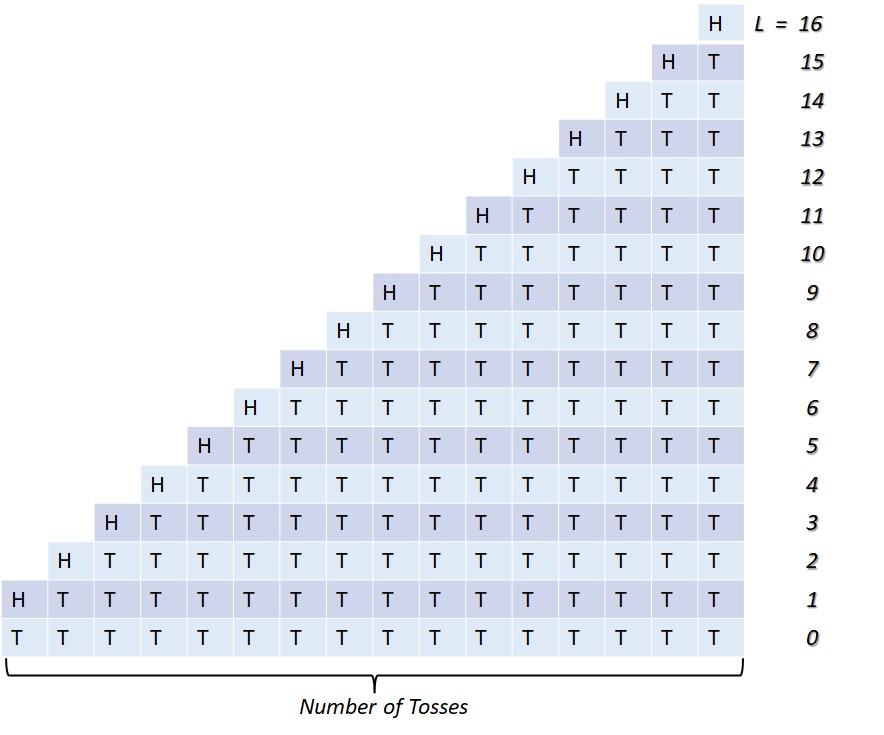
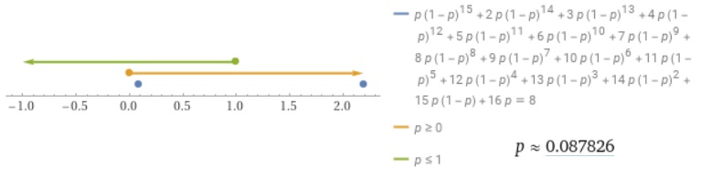
To sub-sample, we assign different levels of quantization to each parameter w while maintaining an average equals to , as discussed above. The randomization factor in selecting the level is modelled as tossing a coin for times. The last toss in which Head occurs indicates the quantization level for the current w, as shown in Figure 1. A fair coin where each outcome has probability is unsuitable to our scheme. It results in , as easily demonstrable through the formula (12), which does not guarantee the desired privacy. To balance the average quantization across all weights and provide the necessary noise we use a biased coin with and guaranteeing . The solution was found by solving the linear system (13) shown in Figure 2.
| (12) |
| (13) |
5 The Negotiation Protocol
In our scheme all participants must securely share the initial parameters of the quantization procedure, namely the selected quantization levels to be used and the enlarged ranges , with ) and ). Many different Multi-Party Computation (MPC) protocols can be used for achieving common knowledge of these parameters without sharing the local feature values or ranges [31]. Below, we describe a secure sharing protocol under the reasonable assumption of a majority of honest participants.
5.1 Secret Sharing
Our protocol utilises the classic technique of Shamir secret sharing [32] to share a secret amongst parties, so that any subset of or more of the parties can reconstruct the secret, yet no subset of or fewer parties can learn anything about the secret. Shamir’s secret sharing scheme relies on the fact that for any for points on the two dimensional plane with unique , there exists a unique polynomial of degree at most such that for every , and that it is possible to efficiently reconstruct the polynomial , or any specific point on it111All computations in this section are in a finite field , for any prime number . In order to share a secret , for example its local , the participant chooses a random polynomial of degree at most under the constraint that .
In practice, each participant sets , chooses random coefficients ,and sets . Then, for every the participant provides the -th party with the share . Note that , so different shares can be given to each party. Reconstruction by a subset of any parties works by interpolating the polynomial to derive and then compute .
Although parties can completely recover , any subset of or fewer parties cannot learn anything about , as they do not have enough points on the polynomial. Since the polynomial is random, all polynomials are equally likely, and all values of are equally likely.
5.2 The MPC protocol
We are now ready to outline the steps of our protocol.
-
1.
Coordinator election. The first conceptual step in our protocol is selecting the coordinating node who will be in charge of deciding the enlargement parameter . In practice, this step can be merged with the next one, as the node in charge of announcing can simply be the one who shared the largest local .
-
2.
Local range sharing: In this step, each party shares its local and with the other parties, using Shamir’s secret sharing.
-
3.
Quantization set-up The coordinator decides the number of quantization levels and carries out the random extraction of the quantization levels to be used in the training.
-
4.
Hyper-parameter sharing The coordinator announces the , , parameters and the extracted quantization levels to the other parties, using Shamir’s secret sharing.
The protocol must be executed before distributed training can begin. It is secure for semi-honest adversaries, as long as less than parties are corrupted[33]. This is because the only values seen by the parties during the computation are secret shares (that reveal nothing about the values they hide). To achieve security in the presence of malicious adversaries who will deviate from the protocol’s specification, it is necessary to rely on specific methods to prevent cheating [34].
5.3 Brute Force attack analysis
Secure sharing of the algorithm parameters is necessary but not sufficient to guarantee privacy through our Hash-Comb encoding. A malicious observer could still crack our algorithm using a brute-force approach to guess the range , hash the values and match the results with the target to validate the guess. It should be noted that the following considerations are intended for normalized values of the training datasets as well as of the learning model parameters.
Because the time complexity of brute force is , where characters in a string of length requires tries, the smallest is the range of values and the more susceptible it is to brute-force attack. The authors in [35] explain that a 128-bit security is well beyond the exhaustive search power of current technology. We can consider a secret on 128-bit computationally secure as to simply iterate through all the possible values requires flips on a conventional processor 222https://en.wikipedia.org/wiki/Brute-force_attack, the Von Neumann-Landauer Limit can be applied to estimate the energy required as joules, which is equivalent to consuming 30 gigawatts of power for one year. This is equal to or which is approximately 0.1% of the yearly world energy production.
Being the hashed value of the channel having range and assuming the use of double-precision floating-point representation (according to the IEEE 754 standard), where a bit is dedicated for the sign, 11 bit for the exponent and 52 bits for the mantissa, the combination of the limits perfectly fits as a shared secret of 128 bits required for the encoding. Unfortunately, due to the nature of the scalars in our scenarios, which are either ML models’ parameters (weights) or normalized features values, the potential attacker could make strong assumptions in guessing those ranges.
For example, the attacker can assume model parameters having and , therefore the merging can be represented using values. More conservative ranges such as and only increase the possible representations to , both assumptions significantly reduce the number of tries for the attacker. In the case of normalized values, the task for the attacker is further simplified by the fact that and are fixed and corresponding to the normalization range itself, and the only effort would be the guess of the enlargement value .
In conclusion, we use an additional number of bits to encode concatenated to the other shared secret to achieve the target of 128-bits to calculate as and to achieve a schema that is brute-force proof.
6 Training Models with Hash-Combs
We start our experimental validation by training a monolithic ML model using multi-quantized training data.
6.1 Datasets
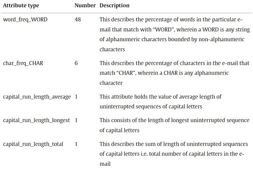
For our experiments, we used three different datasets. The first dataset is part of the UCI Machine Learning Repository [36]. Data consists of information from 4601 email messages, originally used in a study to identify junk email, or “spam”. For all 4601 email messages, the ground truth (”email” or ”spam”) is available, along with the relative frequencies of 57 of the most commonly occurring words and punctuation marks in the email message. Figure 3 shows some of those features. The second dataset, the recent IoT-23 dataset [37], has been created simulating IoT network traffic generated by popular IoT devices, including a Philips HUE smart LED lamp, an Amazon Echo home intelligent personal assistant and a Somfy smart door lock. This dataset includes 23 traffic scenarios, 20 of which are malicious traffic from infected device and 3 are normal traffic. Such flows are labeled ”benign” or ”malign”, with an additional label specifying the attack type. For our experiment, we sampled the data from benign traffic and from malign traffic belonging to two types of attack, PartOfAHorizontalPortScan and Okiru. Finally, the Cardiovascular Disease 333https://www.kaggle.com/datasets/sulianova/cardiovascular-disease-dataset/data dataset consisting of 70000 records of patients data, 11 features divided as factual information, results of medical examination and information given by the patient. The target class represents the risk of a cardiovascular problem.
6.2 ML Model
The ML model used for this experiments is a simple Multi-Layer Perceptron (MLP), implemented in Java 17. Our implementation can be configured to work as monolithic model as well as in federated learning with multiple instances of MLP communicating with a central server for sending/receiving updated weights and implementing FedAvg. The model optimization technique is Stochastic Gradient Descent (SGD) and ReLu is used as activation function. The architecture of our MLP counts 5 hidden layers, configured with neurons respectively. The learning rate is , while the number of epochs for the training depends on the requirements of the model to learn the specific dataset. The hardware is an Intel Core i5-9300H CPU 2.40GHz, 2400 Mhz, 4 Cores/8 Logical Cores. The same configuration for the model and hardware specification were maintained throughout all experiments.
6.2.1 Monolithic Training
The results in Table 2 conveys the performance of the monolithic training over the four datasets after normalization. The accuracy of the results was verified by comparison with the MLPClassifier444https://scikit-learn.org/stable/modules/generated/sklearn.neural_network.MLPClassifier.html availbable in Sklearn, a Python library commonly used in similar research projects which has provided perfectly matching performance, therefore proving the accurateness of our implementation. The purpose of this test is to set a benchmark for the experiments in the following section. In fact, the comparison of the monolithic training with the results of the training paired with privacy preserving methods exemplify the performance improvement or decay of the latter when applied to FL.
Training Testing Dataset Target label Support Epochs Accuracy F1-score Spam Spam 1813/3732 25K 0.8801 0.8804 IoT23-Okiru Malicious 9890/20286 10K 0.9911 0.9911 IoT23-HPS Malicious 7478/18624 40K 0.8280 0.8224 Coronary Cardio 10465/21004 12K 0.6231 0.6231
7 Experiments
We experimented our Hash-Comb representation applied to ML weights, encoded and communicated by local models to the central unit in a FL protocol. The experiments in Section 7.1 aim at comparing different quantization levels of Hash-Comb in order to find the optimal number of quantizers and thus validate the theory as explained in Section 4, while in Section 7.2 the focus is on comparing our approach to the most recent competing methods so as to demonstrate effectiveness through performance juxtaposing.
Regarding the metric, we adopted the score which computes an average of precision and recall. The score is proven to be a valid performance metric when trying to solve binary classification problems as in our experiments.
F1-Score Epochs Spam 6K*4 0.8856 0.7019 0.9084 0.9002 0.8969 IoT23-Okiru 2.5K*4 0.9938 0.9870 0.9935 0.9941 0.9941 IoT23-HPS 12K*4 0.8226 0.6255 0.7577 0.8256 0.8224 Coronary 3K*4 0.6217 0.5960 0.6157 0.6229 0.6223
7.1 Federated Learning with Hash-Combed parameters
We replicated rhe monolithic training in Table 2 in a federated environment by deploying 4 instances of MLP communicating with the central unit for averaging. At each round, each local model is trained with exactly 25% of randomly selected samples from the original set, the weights are sent to the central unit once a training step is completed. The purpose of the following 2 experiments is to verify the impact of Hash-Comb on the overall training and also to capture its performance by varying the number of quantizers.
When the weights are sent in clear (), the standard FedAvg Algorithm (14) is applied on the central unit. While using Hash-Comb (), the quantization described in Section 4 is applied based on the initial range and a sequence of hashes is generated for each at every round. The encoding that we use for the experiments is defined as where , it represents the hashing function applied to , the channel at level containing . This encoding is used in (15), implemented in the central unit to compute the encoded average of the received hashed values.
7.1.1 Experiment 1: Bounded communication rounds
The first experiment’s aftermath is outlined in Table 3. It appears immediately evident a slight improvement resulting from the mere exploitation of the FL protocol () when compared with the monolithic training, an outcome that has been widely reported in the literature.
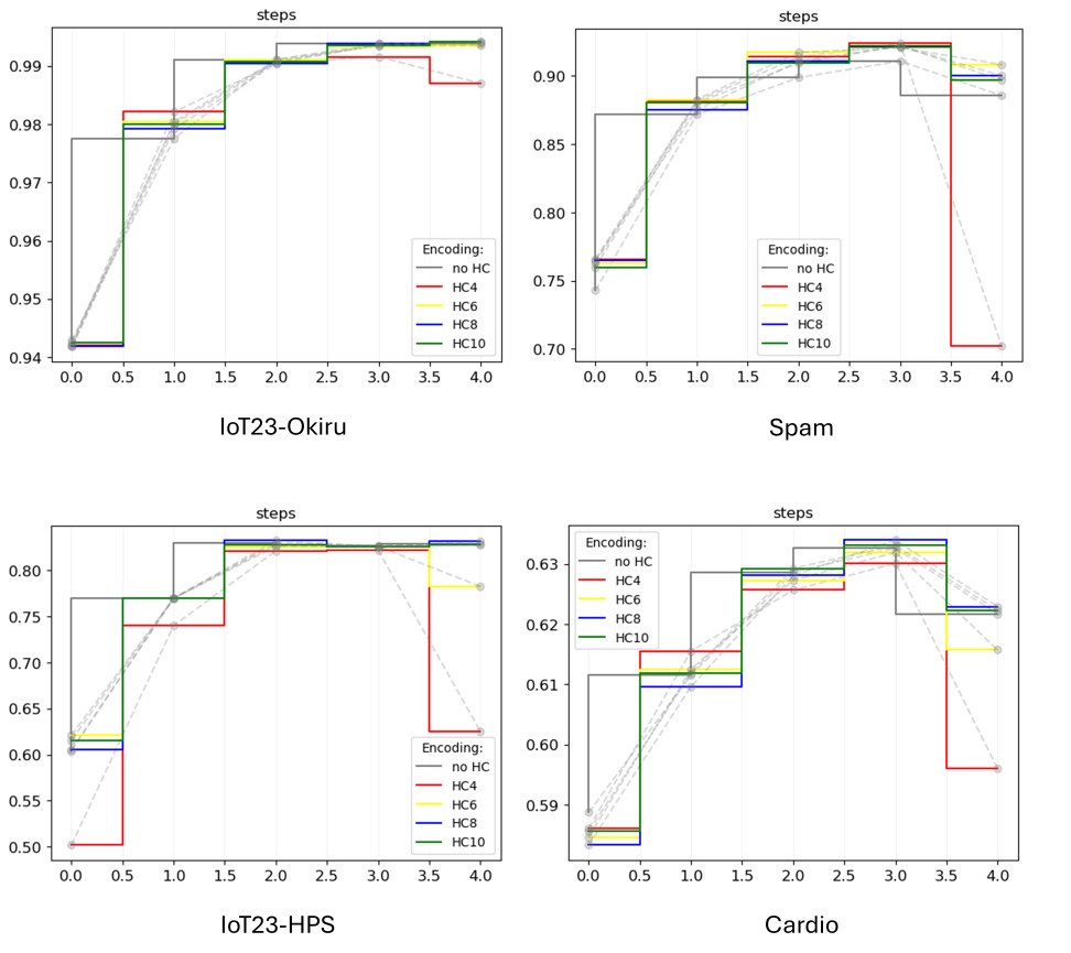
Most importantly, the use of Hash-Comb distinctly reveals a significant improvement with quantization levels, in particular when the model enhances its performances across all datasets. Furthermore, the diagrams in Figure 4 suggest a major over-fitting due to the excessive rounding of the weights when is lower than 8. In conclusion, these findings confirms as a magic number for quantization as previously theorized in Section 4.
| (14) |
| (15) |
7.1.2 Experiment 2: Incremental number of communication rounds
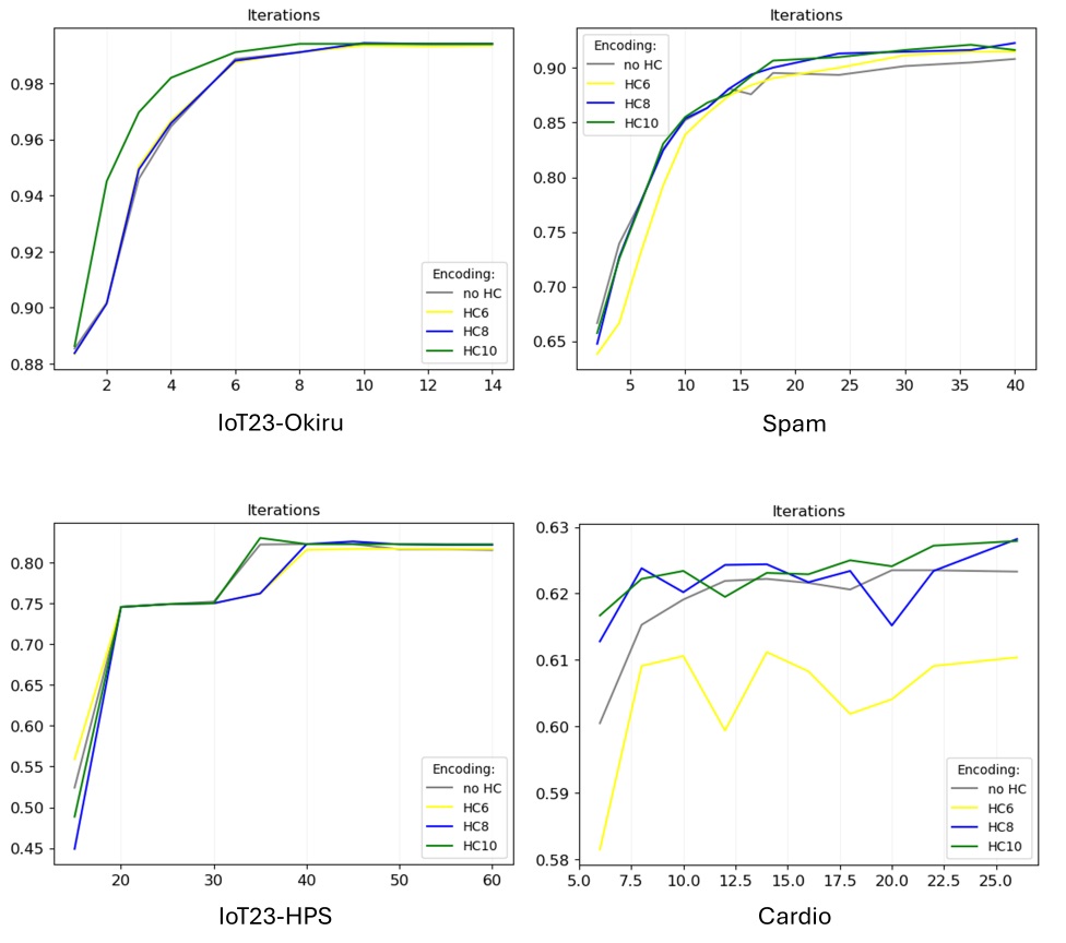
The second set of experiments (see Table 4) has the objective of evaluating the use of Hash-Comb by increasing the frequency of communication rounds and, consequently, the number of FedAvg iterations over the same total number of epochs as before.
Each score within the diagrams in Figure 5 is obtained by validating the general model at each round of communication, confirming the observations previously pointed out: the model using Hash-Comb with achieves better results in the performance and sometimes is a faster learner when compared with non-quantized weights. Some minor instability is observed within the Coronary dataset, probably due to insufficient data quality. In this case, averaging and rounding of the weights may cause fluctuating performance, noticeably for low values, though it eventually converges at the end of the training. This last observation suggests a possible correlation between the value and some measure of training data quality [38].
F1-Score Epochs Spam 1K*40 0.9082 (40) 0.9148 (36) 0.9228 (40) 0.9212 (36) IoT23-Okiru 1K*14 0.9941 (10) 0.9935 (10) 0.9944 (10) 0.9941 (8) IoT23-HPS 1K*60 0.8224 (40) 0.8164 (55) 0.8221 (50) 0.8299 (35) Coronary 1K*26 0.6235 (20) 0.6104 (26) 0.6282 (26) 0.6279 (26)
7.2 Experiment 3: Comparison with classic DP
In this Section our method is compared to a competing approach [39] functionally close to ours which is an ideal benchmark for our proposal. In fact, while the majority of related works focus on FedSGD the method in the above mentioned work adds standard differential privacy (DP) to the FedAvg algorithm. The authors claim that to achieve the desired -DP, the required noise level is:
| (16) |
| (17) |
The is so-called global sensitivity of function and being and a neighboring datasets on the node k, then:
| (18) |
The equation in (18) represents the global sensitivity which is calculated as , where is the number of SGD updates within each communication round, is the ratio between Q and the rows in the dataset and is the clipped local gradient on node , whereas the learning rate is . Based on the experiments mentioned in [39] and also on some preliminary tests we conducted on a training set with added Gaussian noise, the desirable variance is . In fact, a lower value does not guarantee the required privacy while a higher volume of noise significantly reduces the usability of the weights, resulting in a compromised learning outcome.
In our experiment we aim at providing high protection level of -DP while retaining an acceptable usability of the weights. After plugging the above values into Formula (16), setting and a constant , the desired is obtained with q = , establishing a suitable number of gradient updates per communication round given the dataset size .
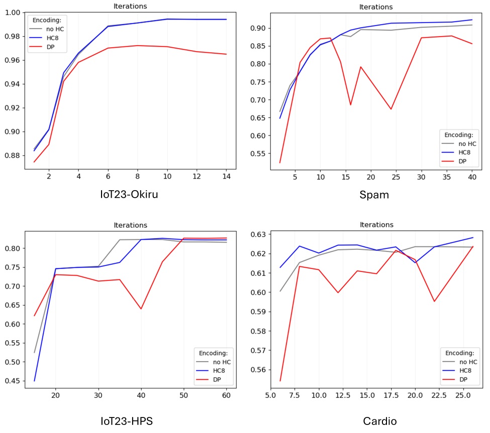
The derived -DP is applied to the training of our datasets for a direct comparison and the results are overlapped to ours and showed in Figure 6. From the analysis of the graphs it is immediately clear that despite a lower volume of noise, compensated by the high frequency of communications, the achieving of a desired DP level leads to a significant degradation of the model, both in terms of performance as well as learning convergence.
Finally, the results in Table 5 show the performance gaining of our Hash-Comb (), featuring an average improvement of in the F1-Score when compared to standard training and of when compared to -DP.
| F1-Score | ||||
|---|---|---|---|---|
| Epochs | ()-DP | |||
| Spam | 40K | 0.9082 (40) | 0.8777 (36) | 0.9228 (40) |
| IoT23-Okiru | 14K | 0.9941 (10) | 0.9721 (8) | 0.9944 (10) |
| IoT23-HPS | 60K | 0.8224 (40) | 0.8264 (60) | 0.8221 (50) |
| Coronary | 26K | 0.6235 (20) | 0.6236 (26) | 0.6282 (26) |
8 Conclusion and Outlook
While data privacy is often mentioned as the motivation for Federated Learning schemes, many popular techniques for federated ML models training cannot yet achieve certifiable privacy and confidentiality. Also, they are often clumsy to implement. We described a novel procedure that smoothly combines randomized quantization to achieve differential privacy and multi-hashing (using standard, regulation-compliant hashes) to provide privacy, confidentiality and regulatory compliance. We empirically studied the performance of our technique and demonstrated that, compared to classic Differential Privacy approaches, it delivers an improved privacy-accuracy trade-off and a much smaller footprint.
Acknowledgement
We would like to express our sincere appreciation to ASPIRE for their financial support (Award Number AARE21-366).
References
- Pugliese et al. [2021] R. Pugliese, S. Regondi, R. Marini, Machine learning-based approach: Global trends, research directions, and regulatory standpoints, Data Science and Management 4 (2021) 19–29.
- El Mestari et al. [2024] S. Z. El Mestari, G. Lenzini, H. Demirci, Preserving data privacy in machine learning systems, Computers & Security 137 (2024) 103605.
- Jegorova et al. [2022] M. Jegorova, C. Kaul, C. Mayor, A. Q. O’Neil, A. Weir, R. Murray-Smith, S. A. Tsaftaris, Survey: Leakage and privacy at inference time, IEEE Transactions on Pattern Analysis and Machine Intelligence (2022).
- Caroline et al. [2020] B. Caroline, B. Christian, B. Stephan, B. Luis, D. Giuseppe, E. Damiani, H. Sven, L. Caroline, M. Jochen, D. C. Nguyen, et al., Artificial intelligence cybersecurity challenges; threat landscape for artificial intelligence, 2020.
- Mauri and Damiani [2021] L. Mauri, E. Damiani, Stride-ai: An approach to identifying vulnerabilities of machine learning assets, in: 2021 IEEE International Conference on Cyber Security and Resilience (CSR), IEEE, 2021, pp. 147–154.
- Caroline et al. [2021] B. Caroline, B. Christian, B. Stephan, B. Luis, D. Giuseppe, E. Damiani, H. Sven, L. Caroline, M. Jochen, D. C. Nguyen, et al., Securing machine learning algorithms, 2021.
- Youn et al. [2023] Y. Youn, Z. Hu, J. Ziani, J. Abernethy, Randomized quantization is all you need for differential privacy in federated learning, 2023. arXiv:2306.11913.
- Almahmoud et al. [2022] A. Almahmoud, E. Damiani, H. Otrok, Hash-comb: A hierarchical distance-preserving multi-hash data representation for collaborative analytics, IEEE Access 10 (2022) 34393–34403.
- Cimato and Damiani [2018] S. Cimato, E. Damiani, Some ideas on privacy-aware data analytics in the internet-of-everything, From Database to Cyber Security: Essays Dedicated to Sushil Jajodia on the Occasion of His 70th Birthday (2018) 113–124.
- Dwork [2006] C. Dwork, Differential privacy, in: International colloquium on automata, languages, and programming, Springer, 2006, pp. 1–12.
- Dwork [2008] C. Dwork, Differential privacy: A survey of results, in: International conference on theory and applications of models of computation, Springer, 2008, pp. 1–19.
- Ghosh et al. [2009] A. Ghosh, T. Roughgarden, M. Sundararajan, Universally utility-maximizing privacy mechanisms, in: Proceedings of the forty-first annual ACM symposium on Theory of computing, 2009, pp. 351–360.
- Chen et al. [2011] R. Chen, N. Mohammed, B. C. Fung, B. C. Desai, L. Xiong, Publishing set-valued data via differential privacy, Proceedings of the VLDB Endowment 4 (2011) 1087–1098.
- Leoni [2012] D. Leoni, Non-interactive differential privacy: a survey, in: Proceedings of the First International Workshop on Open Data, 2012, pp. 40–52.
- Dwork et al. [2006] C. Dwork, F. McSherry, K. Nissim, A. Smith, Calibrating noise to sensitivity in private data analysis, in: Theory of Cryptography: Third Theory of Cryptography Conference, TCC 2006, New York, NY, USA, March 4-7, 2006. Proceedings 3, Springer, 2006, pp. 265–284.
- Dong et al. [2022] J. Dong, A. Roth, W. J. Su, Gaussian differential privacy, Journal of the Royal Statistical Society Series B: Statistical Methodology 84 (2022) 3–37.
- McSherry and Talwar [2007] F. McSherry, K. Talwar, Mechanism design via differential privacy, in: 48th Annual IEEE Symposium on Foundations of Computer Science (FOCS’07), 2007, pp. 94–103. doi:10.1109/FOCS.2007.66.
- Lyu [2022] X. Lyu, Composition theorems for interactive differential privacy, Advances in Neural Information Processing Systems 35 (2022) 9700–9712.
- Dwork et al. [2014] C. Dwork, A. Roth, et al., The algorithmic foundations of differential privacy, Foundations and Trends® in Theoretical Computer Science 9 (2014) 211–407.
- Mironov [2017] I. Mironov, Rényi differential privacy, in: 2017 IEEE 30th computer security foundations symposium (CSF), IEEE, 2017, pp. 263–275.
- Zong et al. [2021] H. Zong, Q. Wang, X. Liu, Y. Li, Y. Shao, Communication reducing quantization for federated learning with local differential privacy mechanism, in: 2021 IEEE/CIC International Conference on Communications in China (ICCC), 2021, pp. 75–80. doi:10.1109/ICCC52777.2021.9580315.
- Yan et al. [2023] G. Yan, T. Li, K. Wu, L. Song, Killing two birds with one stone: Quantization achieves privacy in distributed learning, arXiv preprint arXiv:2304.13545 (2023).
- Agarwal et al. [2018] N. Agarwal, A. T. Suresh, F. X. X. Yu, S. Kumar, B. McMahan, cpsgd: Communication-efficient and differentially-private distributed sgd, in: S. Bengio, H. Wallach, H. Larochelle, K. Grauman, N. Cesa-Bianchi, R. Garnett (Eds.), NIPS’18: Proceedings of the 32nd International Conference on Neural Information Processing Systems, Curran Associates, Inc., 2018, p. 7575–7586.
- Yan et al. [2023] G. Yan, T. Li, T. Lan, K. Wu, L. Song, Layered randomized quantization for communication-efficient and privacy-preserving distributed learning, arXiv preprint arXiv:2312.07060 (2023).
- Frane [1998] J. W. Frane, A method of biased coin randomization, its implementation, and its validation, Drug Information Journal: DIJ/Drug Information Association 32 (1998) 423–432.
- Agrawal et al. [2019] R. Agrawal, Y.-H. Chen, T. Horel, S. Vadhan, Unifying computational entropies via kullback–leibler divergence, in: Annual International Cryptology Conference, Springer, 2019, pp. 831–858.
- Van Erven and Harremos [2014] T. Van Erven, P. Harremos, Rényi divergence and kullback-leibler divergence, IEEE Transactions on Information Theory 60 (2014) 3797–3820.
- Roychowdhury and Roychowdhury [2022] L. Roychowdhury, M. K. Roychowdhury, Quantization for a probability distribution generated by an infinite iterated function system, 2022. arXiv:1603.00731.
- Liu and Talwar [2019] J. Liu, K. Talwar, Private selection from private candidates, in: Proceedings of the 51st Annual ACM SIGACT Symposium on Theory of Computing, 2019, pp. 298–309.
- Papernot and Steinke [2021] N. Papernot, T. Steinke, Hyperparameter tuning with renyi differential privacy, arXiv preprint arXiv:2110.03620 (2021).
- Lindell [2020] Y. Lindell, Secure multiparty computation (mpc), Cryptology ePrint Archive, Paper 2020/300, 2020. URL: https://eprint.iacr.org/2020/300. doi:10.1145/3387108, https://eprint.iacr.org/2020/300.
- Shamir [1979] A. Shamir, How to share a secret, Communications of the ACM 22 (1979) 612–613.
- Veugen et al. [2015] T. Veugen, F. Blom, S. J. de Hoogh, Z. Erkin, Secure comparison protocols in the semi-honest model, IEEE Journal of Selected Topics in Signal Processing 9 (2015) 1217–1228.
- Ishai et al. [2009] Y. Ishai, M. Prabhakaran, A. Sahai, Secure arithmetic computation with no honest majority, in: Theory of Cryptography: 6th Theory of Cryptography Conference, TCC 2009, San Francisco, CA, USA, March 15-17, 2009. Proceedings 6, Springer, 2009, pp. 294–314.
- Tezcan [2022] C. Tezcan, Key lengths revisited: Gpu-based brute force cryptanalysis of des, 3des, and present, Journal of Systems Architecture 124 (2022) 102402. URL: https://www.sciencedirect.com/science/article/pii/S1383762122000066. doi:https://doi.org/10.1016/j.sysarc.2022.102402.
- Hopkins et al. [1999] M. Hopkins, E. Reeber, G. Forman, J. Suermondt, Spambase, UCI Machine Learning Repository, 1999. DOI: https://doi.org/10.24432/C53G6X.
- Sebastian Garcia [2020] . M. J. E. Sebastian Garcia, Agustin Parmisano, Iot-23: A labeled dataset with malicious and benign iot network traffic (version 1.0.0) [data set]. zenodo. http://doi.org/10.5281/zenodo.4743746, 2020.
- Mauri and Damiani [2021] L. Mauri, E. Damiani, Estimating degradation of machine learning data assets, ACM Journal of Data and Information Quality (JDIQ) 14 (2021) 1–15.
- Li et al. [2020] Y. Li, T.-H. Chang, C.-Y. Chi, Secure federated averaging algorithm with differential privacy, in: 2020 IEEE 30th International Workshop on Machine Learning for Signal Processing (MLSP), 2020, pp. 1–6. doi:10.1109/MLSP49062.2020.9231531.