Dynamically Consistent Analysis of Realized Covariations in Term Structure Models

Dennis Schroers Institute of Finance and Statistics and Hausdorff Center for Mathematics
University of Bonn
Abstract.

In this article we show how to analyze the covariation of bond prices nonparametrically and robustly, staying consistent with a general no-arbitrage setting. This is, in particular, motivated by the problem of identifying the number of statistically relevant factors in the bond market under minimal conditions. We apply this method in an empirical study which suggests that a high number of factors is needed to describe the term structure evolution and that the term structure of volatility varies over time.

Key words and phrases:
Keywords: Term Structure Models, Principal Component Analysis, Functional Data Analysis, Jumps, Bond Market

1. Introduction

We present a nonparametric method to measure covariations in a general arbitrage-free term structure setting in the spirit of [9]. A motivation is to determine the number of statistically relevant random drivers needed to describe bond market dynamics under minimal assumptions and in a dynamically consistent manner. That is, by working coherently in the abstract setting of [9], we circumenvent the well-known consistency problems of finding arbitrage-free finite-dimensional dynamics that reflect the empirical observations.

In the bond market the notion of a zero coupon bond is fundamental. A zero coupon bond guarantees its holder at time $t$ a fixed amount of money at some time $t+x$ in the future. The cost $P_{t}(x)$ of entering this contract at time $t$ is the price of this bond, which depends on the time to maturity $x$, implying a price curve $x\mapsto P_{t}(x)$ at each time $t\geq 0$ called the discount curve. We assume to observe bond price or yield curve data, potentially derived by smoothing as in [22] or [31], such that we can recover log bond prices

$$P_{i,j}^{n}:=\log P_{i\Delta_{n}}(j\Delta_{n})\quad j=0,1,...,\lfloor M/\Delta_{n}\rfloor,\,\,i=0,1,...,\lfloor T\Delta_{n}\rfloor$$

for a resolution $\Delta_{n}=1/n$ and with different maturities $j\Delta_{n}$ and on different time points $i\Delta_{n}$. Here $M>0$ is some maximal time to maturity (e.g. $M=10$ or $M=30$ when time is measured in years) and $T$ is the time until which the data are observed or considered.

Often, risk factor analyses are conducted on the basis of transformations of the discount curve, such as yield differences or excess returns, which typically suggests that three factors explain a large amount of variation in bond market dynamics, c.f. [30]. Recently [15], raised the concern that these low-dimensional factor structures are obtained irrespectively of the data generating process due to the high correlation of bond prices with close maturities. To remedy this effect, dimension reduction could be based on difference returns, which are the returns of the trading strategy of buying an $x+\Delta$-maturity bond and shorting an $x$-maturity bond. Precisely, difference returns are defined for $i=1,...,\lfloor T/\Delta_{n}\rfloor-1$ and $j=1,...,\lfloor M/\Delta_{n}\rfloor-1$ by

(1) $\displaystyle d_{i}^{n}(j):=P_{i+1,j}^{n}-P_{i,j+1}^{n}-P_{i+1,j-1}^{n}+P_{i,j}^{n}.$

In this article we develop an asymptotic econometric theory for the realized covariations of these difference returns, that is, for $j_{1},j_{2}=1,...,\lfloor M/\Delta_{n}\rfloor$ we analyse the covariations

$$\hat{q}_{T}^{n}(j_{1},j_{2}):=\sum_{i=1}^{\lfloor T/\Delta_{n}\rfloor}d_{i}(j_{1})d_{i}(j_{2}).$$

Importantly, while $\lfloor T/\Delta_{n}\rfloor^{-1}q_{T}^{n}$ is the empirical covariance of the data $d_{1}^{n},...d_{\lfloor T/\Delta_{n}\rfloor-1}^{n}$, assuming w.l.o.g. $\mathbb{E}[d_{i}^{n}]=0$, we do not consider it as an estimator of the population covariance of difference returns. Such an interpretation is not invariant with respect to the resolution $\Delta_{n}$ and requires the restrictive assumption that difference returns are i.i.d. or at least covariance stationary and ergodic. More importantly, it is not clear how dimension reduction can be conducted without entailing arbitrage opportunities. General arbitrage-free term structure models in the sense of [10] and [23] require that forward rates $f_{t}(x)=-\partial_{x}\log(P_{t}(x))$ for $x,t\geq 0,$ satisfy dynamics of the form

(2) $\displaystyle df_{t}=\partial_{x}f_{t}dt+dX_{t},\quad t\geq 0.$

where the equation holds in an appropriate function space. The latent process $X$ is a possibly infinite-dimensional Itô semimartingale

$$X_{t}:=\int_{0}^{t}\alpha_{s}ds+\int_{0}^{t}\sigma_{s}dW_{s}+J_{t}.$$

where $\alpha$ is a curve-valued drift process, $\sigma$ is the (in general operator-valued) volatility, $W$ is an (in principle infinite-dimensional) Wiener process and $J$ is a jump process that we assume to model rare extreme events (c.f. Section A for the details). Under a risk-neutral measure, the drift $\alpha$ can in addition be characterized as a deterministic function of the volatility $\sigma$ and characteristics of the jump process $J$ (c.f. [10], [23]). Parametrizations of forward cuves are then required to be viable in the dynamic setting (2) to avoid the introduction of arbitrage opportunities to the model. This is known to be an intricate problem in term structure modelling (see e.g. [9], [11], [24], [21], [20]) and some frequently employed parametrizations of forward curves are incompatible with arbitrage-free dynamics or induce restrictive additional conditions (see e.g. [19]).

The concerns on realized covariations of difference returns can be resolved when we consider infill asymptotics ($n\to\infty$). Precisely, we show without imposing further assumptions and interpreting $\hat{q}_{T}^{n}$ as a piecewise constant kernel that

(3) $$\lim_{n\to\infty}\Delta_{n}^{-2}\hat{q}_{T}^{n}(\lfloor x/\Delta_{n}\rfloor,\lfloor y/\Delta_{n}\rfloor)=\lim_{n\to\infty}\sum_{i=1}^{\lfloor T/\Delta_{n}\rfloor}\Delta_{i}^{n}X(x)\Delta_{i}^{n}X(y),$$

where the limits hold in $L^{2}([0,M]^{2})$. The right hand side describes the quadratic covariation of the latent driver $X$, which always exists (see e.g. [44]) and can equivalently be described as the limit of covariance operators in $L^{2}(\mathbb{R}_{+})$ by

(4) $$[X,X]_{t}:=\lim_{\Delta_{n}\downarrow 0}\sum_{i=1}^{\lfloor t/\Delta_{n}\rfloor}\langle\Delta_{i}^{n}X,\cdot\rangle\Delta_{i}^{n}X,$$

where $\langle\cdot,\cdot\rangle$ is the inner product of $L^{2}(\mathbb{R}_{+})$ and $\Delta_{i}^{n}X:=X_{i\Delta_{n}}-X_{(i-1)\Delta_{n}}$ denotes the $i$’th increment of $X$.

The limit (3) implies that it is possible to infer on the number of random drivers in the bond market on the basis of discrete bond price data without further assumptions on moments, stationarity and ergodicity. In fact, if the quadratic variation of $X$ is $d$-dimensional for $d\in\mathbb{N}$, then $X$ is $d$-dimensional and its state space (until time $T$) is spanned by the eigenvectors corresponding to the nonzero eigenvalues of $[X,X]_{T}$. The eigenvalues of $[X,X]_{T}$ indicate the amount of variation that the corresponding random factor explained of $X$ up to time $T$. This is in contrast to the explained variation of factors derived from a covariance of $f$ or its increments, which is a priori not informative on the number of random drivers. In fact, it is possible that $f$ is infinite-dimensional, while $X$ is a one-dimensional process (c.f. Example 4.1 in [44]). The most striking advantage of the interpretation of the realized covariation of difference returns in (3) is, however, that exchanging $X$ by an arbitrary finite-dimensional semimartingale (with the correct form of the drift) in the formulation of the dynamics in (2) does not affect the capability of the model to be free of arbitrage, such that an investigation of the number of relevant factors can be conducted independently of further consistency conditions. This underlines that our abstract infinite-dimensional setting relaxes the analysis of the term structure when compared to models in which state spaces are assumed to be finite-dimensional a priori. An additional advantage of quadratic variations is that they are naturally interpreted as time-varying objects enabling their temporal analysis.

In practice, the distortion of the measurements due to ouliers can bias the analysis of the relevant factors. For instance, in the context of sudden interest rate movements during an economic crisis it is possible that a single outlying difference return impacts the measurement of covariations and, thus, the measured dimensionality of the driver $X$ substantially. For this reason, besides $[X,X]$, the continuous part $[X^{C},X^{C}]$ of the quadratic variation where $X^{C}_{t}=\int_{0}^{t}\alpha_{s}ds+\int_{0}^{t}\sigma_{s}dW_{s}$ is central for the task of identifying the statistically relevant number of random drivers, considering the jump part to model outlying events. We describe how estimation of the continuous quadratic covariation is possible by a truncation technique, which sets outlying difference returns in the realized covariation on the left of (3) to 00. We derive rates of convergence and a central limit theorem for these estimators and also show how the long-time limit of $[X^{C},X^{C}]_{T}/T$ as $T\to\infty$ can be estimated, if it exists. Our limit theory holds under weak assumptions, which mainly reflect those for finite-dimensional semimartingales, although, $f$ does not need to be a semimartingale.

We conduct an emprical study on the relevant drivers in the market via this covariation estimates based on real bond market data. The procedure is numerically equivalent to a principal component analysis based on the (truncated) empirical covariance of difference returns with a daily resolution and mean zero. However, the classification of jumps takes into account the abstract setting (2). By investigation of a truncated version of the realized covariations $q_{j}^{*}(x,y):=\Delta_{n}^{-2}\sum_{i=\lfloor(j-1)/\Delta_{n}\rfloor}^{\lfloor j/\Delta_{n}\rfloor}d_{i}(\lfloor x/\Delta_{n}\rfloor)d_{i}(\lfloor y/\Delta_{n}\rfloor)$ for any year $j$ from 1990 to 2022, we find evidence for the dimension of the driver to vary from year to year but also to be consistently high (in each year more than $8$ drivers are needed to explain at least $99\%$ of the variation). We further observe that quadratic variations vary in shape over time and not just their level. We provide Monte-Carlo evidence for the validity of the limit theory in the context of sparse and noisy data.

Formal validity of our method is guaranteed by relating difference returns via cross-sectional and temproal discretization to the abstract setting (2) and then apply the results from the article [44]. The truncation procedure is inspired from the truncated realized variation estimators of [32, 33, 34] and [27] for finite-dimensional semimartingales. Here, we also provide a data-driven variant of the truncation rule, to account for functional outliers in a similar way as the trimmed least squares method in [42]. Naturally, our asymptotic theory also allows for nonparametric estimation of characteristics of infinite-dimensional volatility models in continuous time employed for term structure modeling (c.f. [4], [8], [7], [14], [13], [3] and [12]).

The article is structured as follows: Section 2 describes the general bond market setting that we consider for this article. Section 3 presents the estimation theory for the central application of term structure models. Identification for the quadratic variations of $X$, $X^{C}$ and $J$ on the basis of difference return variations can be found in Section 3.1, while rates of convergence for estimating $[X^{C},X^{C}]$ and a central limit theorem can be found in Section 3.3. Section 3.3.1 discusses long-time asynmptotics for estimation of a stationary mean of $[X^{C},X^{C}]_{T}/T$. Section 3.4 contains practical considerations on smoothing of discrete bond price data and presents a data-driven truncation rule for robust estimation. Section 4 provides a simulation study. Finally, we apply our theory to bond market data in Section 5. Technical proofs of our results along with further remarks on the simulation scheme and additional empirical results can be found in the appendix.

1.1. Technical preliminaries and notation

Let $I$ be an interval in $\mathbb{R}$. We write $\langle h,g\rangle=\int_{I}h(x)g(x)dx$ for the $L^{2}$-scalar product of two elements $h,g\in L^{2}(I)$ as well as $\|h\|=\sqrt{\langle h,h\rangle}$ for the norm. We write $L_{\text{HS}}(L^{2}(I))$ for the Hilbert space of Hilbert-Schmidt operators from $L^{2}(I)$ into itself and $\|\mathcal{T}_{k}\|_{\text{HS}}$ for the Hilbert-Schmidt norm of an $\mathcal{T}_{k}\in L_{\text{HS}}(L^{2}(I))$. Recall, that a Hilbert-Schmidt operator $\mathcal{T}_{k}:L^{2}(I)\to L^{2}(I)$ can be uniquely associated to a kernel $k\in L^{2}(I^{2})$ such that $\|\mathcal{T}_{k}\|_{\text{HS}}=\|k\|_{L^{2}(I^{2})}$ and

(5) $$\mathcal{T}_{k}f(x)=\int_{I}k(x,y)f(y)dy\quad\forall f\in L^{2}(I).$$

Importantly, the operator $h\otimes g:=\langle h,\cdot\rangle g$ is Hilbert-Schmidt for two elements $h,g\in L^{2}(I)$. We shortly write $h^{\otimes 2}=h\otimes h$. Finally, for $L^{2}(I)$-valued processes $X^{n},n\in\mathbb{N}$, $X$, we write $X^{n}\stackrel{{\scriptstyle u.c.p.}}{{\longrightarrow}}{X}\quad\text{ as }n\to\infty$ for the convergence uniformly on compacts in probability, i.e. it is $\mathbb{P}[\sup_{t\in[0,T]}\|X^{n}(t)-X(t)\|>\epsilon]\to 0$ for all $\epsilon,T>0$.

2. General Arbitrgae-Free Bond Market-Dynamics

Let $(\Omega,\mathcal{F},(\mathcal{F}_{t})_{t\geq 0},\mathbb{P})$ be a filtered probability space with right-continuous filtration. From here on, we assume that the forward rate process $(f_{t})_{t\geq 0}$ is an $L^{2}(\mathbb{R}_{+})$-valued stochastic process that is the mild solution to the stochastic partial differential equation (2), defined on $(\Omega,\mathcal{F},(\mathcal{F}_{t})_{t\geq 0},\mathbb{P})$. That is,

(6) $\displaystyle f_{t}=$ $\displaystyle\mathcal{S}(t)f_{0}+\int_{0}^{t}\mathcal{S}(t-s)\alpha_{s}ds+\int_{0}^{t}\mathcal{S}(t-s)\sigma_{s}dW_{s}+\int_{0}^{t}\mathcal{S}(t-s)dJ_{t}.$

where $\mathcal{S}(t)f(x)=f(x+t)$ for $t\geq 0$ and $f\in L^{2}(\mathbb{R}_{+})$ defines the left-shift operator semigroup. We relegate all further technical discussions on $X$, $\alpha$, $\sigma$, $W$ and $J$ and various related technical assumptions that we need in for the validity of our limit theory to Sections A in the appendix. We remark, that under arbitrage-free dynamics, that is, under an equivalent local martingale measure the drift is necessarily a deterministic function of $\sigma$ and $\gamma$ (c.f. [10]), which was in the continuous case the original inside leading to the popular Heath-Jarrow-Morton framework of [26] for pricing bonds and interest rate sensitive contingent claims. However, this will not be of particular importance for our purposes, as the drift later vanishes asymptotically in our limit theory. We will discuss however some important examples subsequently. Before that, we make a remark on the choice $L^{2}(\mathbb{R}_{+})$ as the state space of forward rate curves.

Remark 2.1 (On the forward curve space).

There are other choices for the state space of $f$ than $L^{2}(\mathbb{R}_{+})$ such as the forward curve space of [21]. We choose, however, to work in an $L^{2}$-setting because in that way we do not impose further regularity assumptions on the forward curves. A supposed restriction of the state space $L^{2}(\mathbb{R}_{+})$ is that the so-called long-rates $\lim_{x\to\infty}f_{t}(x)$ are equal to 00. This is undesirable from a financial point of view and could easily be fixed in several ways. For instance, we could consider the Hilbert space $H:=\mathbb{R}\oplus L^{2}(\mathbb{R}_{+})=\{f:\mathbb{R}_{+}\to\mathbb{R}:f(x)=a+h(x),a\in\mathbb{R},h\in L^{2}(\mathbb{R}_{+})\}$, for which the first component models the long-rate. In this case, the forward curve space of [21] would be contained as a subspace. We then might just assume that the state spaces of $X^{C}$ and $J$ belong to $\{0\}\times L^{2}(\mathbb{R}_{+})\equiv L^{2}(\mathbb{R}_{+})$, which is in line with the assumptions on the volatilities in [23]. As $[X,X]$, $[X^{C},X^{C}]$ and $[J,J]$ do not depend on the drift and the initial condition, the respective limit theory would be exactly the same. Another reason that justifies our choice is that in practice, our asymptotic analysis just takes into account bond price data $P_{t}(x)$ with $(t,x)\in[0,T]\times[0,M]\subset\mathbb{R}_{+}^{2}$ for some maximal time to maturity $M<\infty$ and the behavior of the forward curves for $x\to\infty$ is of minor importance. To relax the notation, we stick to the state space $L^{2}(\mathbb{R}_{+})$ without loss of generality.

Let us now discuss some important simple examples.

Example 2.2.

[Sum of $Q$-Wiener and compound Poisson process] As a simple example assume $\alpha_{t}=\alpha\in L^{2}(\mathbb{R}_{+})$ and $\sigma_{t}=\sigma\in L_{\text{HS}}(\mathbb{R}_{+})$ to be constant. Then, $X^{C}_{t}$ is a Gaussian random variable in $L^{2}(\mathbb{R}_{+})$ with mean $t\alpha$ and covariance $tQ:=t\sigma\sigma^{*}$, where $\sigma^{*}$ is the Hilbert space adjoint of $\sigma$. equivalently, $X_{t}^{C}$ has covariance kernel $q$ given by $\int_{\mathbb{R}_{+}}q(x,y)f(y)dy=(Qf)(x)$ for $x\geq 0$. Since we want use the jump process to model rare outliers, a reasonale model would be a compound Poisson process

$$J_{t}:=\sum_{i=1}^{N_{t}}\chi_{i},$$

for an i.i.d. sequence $(\chi_{i})_{i\in\mathbb{N}}$ of random variables in $L^{2}(\mathbb{R}_{+})$ with law $F$ and finite second moment ($\mathbb{E}[\|\chi_{i}\|^{2}]<\infty$) and a Poisson process $N$ with intensity $\lambda>0$. Since in the technical Section A we require the jump process to be a martingale, this is not immediately a valid choice, but we can rewrite the dynamics accordingly (c.f. Example A.1 in the appendix). The quadratic covariation of this semimartingale is then

$$[X,X]_{t}=[X^{C},X^{C}]_{t}+[J,J]_{t}=tQ+\sum_{i=1}^{N_{t}}\chi^{\otimes 2}_{i}.$$

The term structure setting (2) contains the vast majority of existing arbitrage-free term structure models considered in the literature. Among them is the class of affine term structure models, which are widely appreciated for their parsimony.

Example 2.3 (Affine term structure models).

In an affine term structure model, the state space for forward curves is spanned by a finite amount of factors, such that

(7) $\displaystyle f_{t}(x)=g_{0}(x)+g_{1}(x)x_{t}^{1}+...+g_{d}(x)x_{t}^{d},$

where $g:\mathbb{R}_{+}\to\mathbb{R}$ are some particularly suitable functions and the process $x=(x^{1},...,x^{d})$ is an affine process (c.f. [17]). To guarantee that a factor structure like (7) can be in line with general no arbitrage dynamics of the form (2) one has to impose restrictions on both the functions $g_{0},g_{1},...,g_{d}$ as well as the multivariate semimartingale $x$ (c.f. e.g. [21], Section 7.4 for a description in a continuous setting). If $[x^{c},x^{c}]$ and $[x^{d},x^{d}]$ denote the continuous and discontinuous part of the multivariate quadratic variation of $x$, it is

$$[X^{C},X^{C}]_{t}t=\sum_{i=1}^{d}[x_{i}^{c},x_{j}^{c}]_{t}g_{i}\otimes g_{j},\qquad[J,J]_{t}=\sum_{i=1}^{d}[x_{i}^{d},x_{j}^{d}]_{t}g_{i}\otimes g_{j}.$$

If the respective bond market data are in line with an affine model such as (7), our theory in Section 3 identifies this structure asymptotically.

Let us outline two classical special cases when $d=1$ and when there are no jumps:

  • (a)

    (Vašiček model) In the Vašiček model it is

    $$dx^{1}_{t}=(b-ax_{t}^{1})dt+\sigma_{0}d\beta_{t}$$

    for $b,a,\sigma_{0}>0$ and a one-dimensional Brownian motion $\beta$. The functions $g_{0},g_{1}$ are then given by $g_{1}(x)=e^{-ax}$ and $g_{0}(x)=b\int_{0}^{x}g_{1}(y)dy-(\sigma_{0}^{2}/2)(\int_{0}^{x}g_{1}(y)dy)^{2}$ (c.f. Section 7.4.2 in [21]). In this case, the quadratic variation of the latent driving semimartingale $X$ is

    $$[X,X]_{t}=[f,f]_{t}=t\sigma_{0}^{2}(e^{-a\cdot})^{\otimes 2},\qquad t\geq 0.$$

    With $Q=\sigma_{0}^{2}(e^{-a\cdot})^{\otimes 2}$, this is a special case of Example 2.2 without jumps.

  • (b)

    (CIR model) In the CIR model we have short rate dynamics of the form

    $$dx_{t}^{1}=(b-ar_{t})dt+\sigma_{0}\sqrt{x^{1}_{t}}d\beta_{t}$$

    for $b,a,\sigma_{0}\geq 0$ and a standard univariate Brownian motion $\beta$. The function $g_{1}$ is given as the derivative of the function $x\mapsto G_{1}(x):=2(e^{cx}-1)/((c-a)(e^{cx}-1)+2c)$ with $c=\sqrt{a^{2}-2\sigma_{0}}$ and the function $g_{0}$ is given as $g_{0}=aG_{1}$ (c.f. Section 7.4.1) in [21]). In this case the quadratic variation of the latent driving semimartingale $X$ is

    $$[X,X]_{t}=[f,f]_{t}=\sigma_{0}^{2}\left(\int_{0}^{t}x^{1}_{t}ds\right)g_{1}^{\otimes 2},\qquad t\geq 0.$$

Many simple ways to model term structures lead to nonaffine dynamics, such as

Example 2.4 (Volterra spot rate models).

For many term structure models the quadratic variation of $f$ is not necessarily well-defined, as it must not be a semimartingale. For instance, take the forward rate dynamics of the form

(8) $\displaystyle f_{t}=f_{0}+\int_{0}^{t}\alpha_{s}(\cdot+t-s)ds+\sum_{i=1}^{d}\int_{0}^{t}k_{i}(\cdot+t-s)\sigma_{s}^{i}d\beta_{s}^{i}$

for a multivariate standard Brownian motion $(\beta^{1},...,\beta^{d})$ for some $d\in\mathbb{N}$, a $d$-dimensional volatility $(\sigma^{1},...,\sigma^{d})$ and deterministic kernels $k^{1},...,k^{d}\in L^{2}(\mathbb{R}_{+})$ as well as a drift $\alpha$ which satisfies the HJM condition (c.f. [21]). In this scenario, the underlying driving semimartingale has quadratic variation equalling

$$[X,X]_{t}=\sum_{i=1}^{d}\left(\int_{0}^{t}(\sigma_{s}^{i})^{2}ds\right)k_{i}^{\otimes 2}.$$

Thus, if $\sigma_{s}^{i}=1$ for all $s\geq 0$ and $i\in\mathbb{N}$, this is a special case of Example 2.2 with $Q=\sum_{i=1}^{d}k_{i}^{\otimes 2}$ and without jumps, but it does not always correspond to an affine term structure. In the energy market, for instance, fractional kernels such that $k_{1}(t)=\mathcal{O}(t^{H})$ for $t\to 0$ and $k_{i}\equiv 0$ for $i\geq 2$ are used to model energy spot prices (c.f. [2] or [1]). If we assume that $k_{1}(t)=t^{H}$, $\sigma^{1}\equiv 1$ and $\alpha_{s}\equiv 0$ for $t\in[0,1]$ one can prove that $f_{t}$ is not a semimartingale in $L^{2}(\mathbb{R}_{+})$ and the quadratic variation does not converge as we show in Appendix C.

Example 26 (and also Example 3.16 in [5]) shows that the process $(f_{t})_{t\geq 0}$ is in general not an $L^{2}(\mathbb{R}_{+})$-valued semimartingale. However, all implied bond prices $(P_{t}(T-t))_{0\leq t\leq T}$ are semimartingales for all $T>0$, which is necessary to guarantee the absence of arbitrage in the bond market. Moreover, while the quadratic covariations of $f$ must not be convergent, we show in the next section, in which we present our main results, that the realized covariation of difference returns measures quadratic covariations of the latent driver asymptotically and without further conditions.

3. Estimation of Quadratic Covariations

In this section we present our asymptotic theory for estimation of quadratic variations. We start with the identifiability of $[X,X]$, $[X^{C},X^{C}]$ and $[J,J]$.

3.1. Identification of the quadratic covariation of the latent semimartingale

We rely on infill asymptotics $\Delta_{n}\to 0$ as $n\to\infty$ and recall the definition of the realized covariation $(\hat{q}_{t}^{n})_{t\geq 0}$ as a piecewise constant kernel. That is, for $x\in[(j_{1}-1)\Delta_{n},j_{1}\Delta_{n}]$ and $y\in[(j_{2}-1)\Delta_{n},j_{2}\Delta_{n}]$, $j_{1},j_{2}\in\mathbb{N}$ and $t\geq 0$ we define

(9) $$\hat{q}_{t}^{n}(x,y):=\sum_{i=1}^{\lfloor t/\Delta_{n}\rfloor}d_{i}^{n}(j_{1})d_{i}^{n}(j_{2}).$$

For each $n\in\mathbb{N}$ and $t\geq 0$, we have that $\hat{q}_{t}^{n}\in L^{2}(\mathbb{R}_{+}^{2})$, which follows from the Assumption that forward curves are elements in $L^{2}(\mathbb{R}_{+})$ (c.f. Remark 3.2 below). We now state the general identifiability result for the quadratic covariation of $X$.

Theorem 3.1.

It is as $n\to\infty$ and w.r.t. the Hilbert-Schmidt norm and $\mathcal{T}_{\hat{q}^{n}}$ as in (5)

(10) $$\Delta_{n}^{-2}\mathcal{T}_{\hat{q}^{n}}\overset{u.c.p.}{\longrightarrow}[X,X].$$

As in the case of finite-dimensional semimartingales, we do not have to impose any further conditions to identify the quadratic covariations of the driving semimartingale $X$ although the observable process $(f_{t})_{t\geq 0}$ is not necessarily an $L^{2}(\mathbb{R}_{+})$-valued semimartingale. This is due to the relation of difference returns to semigroup-adjusted forward rate returns, which where shown in [44], [6] and [5] to be well-suited for volatility estimation for processes of the form (6). This relationship is made clear in the next remark.

Remark 3.2.

[Difference returns are discretized semigroup-adjusted increments] The reason for economically motivated difference returns to lead to such a general identifiability result is that difference returns coincide with orthonormal projections onto semigroup-adjusted increments of forward rate curves. That is, we have

$$d_{i}^{n}(j)=-\langle\tilde{\Delta}_{i}^{n}f,\mathbb{I}_{[(j-1)\Delta_{n},j\Delta_{n}]}\rangle.$$

where $\tilde{\Delta}_{i}^{n}f$ denotes the semigroup-adjusted forward rate increment

$$\tilde{\Delta}_{i}^{n}f:=f_{i\Delta_{n}}-\mathcal{S}(\Delta_{n})f_{(i-1)\Delta_{n}}\quad i=1,...,\lfloor T/\Delta_{n}\rfloor.$$

and $(\mathcal{S}(t))_{t\geq 0}$ is the left shift semigroup on $L^{2}(\mathbb{R}_{+})$. Define

(11) $$\Pi_{n,M}h:=n\sum_{j=1}^{\lfloor M/\Delta_{n}\rfloor}\langle h,\mathbb{I}_{[(j-1)\Delta_{n},j\Delta_{n}]}\rangle\mathbb{I}_{[(j-1)\Delta_{n},j\Delta_{n}]}$$

the projection onto $span(\mathbb{I}_{[(j-1)\Delta_{n},j\Delta_{n}]}:j=1,...,\lfloor M/\Delta_{n}\rfloor)$ and observe that

$\displaystyle\Delta_{n}^{-2}\mathcal{T}_{\hat{q}^{n,M}_{t}}=\Pi_{n,M}(SARCV_{t}^{n})\Pi_{n,M},$

where $SARCV_{t}^{n}=\sum_{i=1}^{\lfloor t/\Delta_{n}\rfloor}\tilde{\Delta}_{i}^{n}f^{\otimes 2}$ is the semigroup-adjusted realized covariation, which was shown to be a consistent estimator of $[X,X]_{t}$ in [44] in the presence of jumps and a consistent and asymptotically normal estimator of $[X^{C},X^{C}]$ in [6] and [5] when $J\equiv 0$. This characterization of the realized covariation $\hat{q}^{n}$ also explains the appearance of the scalar $\Delta_{n}^{-2}$ in front of the covariation in (10).

Next, we examine how to identify the continuous part of the quadratic covariation.

3.2. Identification of $[X^{C},X^{C}]$ and $[J,J]$ via truncated covariation estimators

We now turn to the estimation of the continuous part of the quadratic covariation. We will derive jump robust estimators by a truncated form of $\hat{q}_{t}^{n}$ defined by the piecewise constant kernel $\hat{q}^{n,-}_{t}$ given for $x\in[(j_{1}-1)\Delta_{n},j_{1}\Delta_{n}]$, $y\in[(j_{2}-1)\Delta_{n},j_{2}\Delta_{n}]$, $j_{1},j_{2}\in\mathbb{N}$ and $t\geq 0$ by

(12) $\displaystyle\hat{q}^{n,-}_{t}(x,y):=$ $\displaystyle\sum_{i=1}^{\lfloor t/\Delta_{n}\rfloor}d_{i}^{n}(j_{1})d_{i}^{n}(j_{2})\mathbb{I}_{g_{n}\left(d_{i}^{n}/\Delta_{n}\right)\leq u_{n}}$

for $u_{n}=\alpha\Delta_{n}^{w}$, with $w\in(0,1/2)$ and $\alpha>0$ and a particular sequence of truncation functions $g_{n}$ that takes into account only the discrete data $d^{i}_{n}(j)$ for $j\in\mathbb{N}$. Precisely, the corresponding sequence of truncation functions $g_{n}:l^{2}\to\mathbb{R}_{+}$ must satisfy for constants $c,C>0$ and for all $f,h\in l^{2}$ and all $n\in\mathbb{N}$

(13) $\displaystyle c\|f\|_{l^{2}}\leq g_{n}(f)\leq C\|f\|_{l^{2}},\quad\text{ and }\quad g_{n}(f+h)\leq g_{n}(f)+g_{n}(h).$

While the particular choice of the functions $g_{n}$ will not play a role for the asymptotic behavior of $\hat{q}^{n,-}_{t}$, it is important to modify it in practice. For the moment, one can take in mind the legitimate choice $g_{n}=\|\cdot\|_{l^{2}}$ for all $n\in\mathbb{N}$ for which we have with $\Pi_{n,\infty}$ defined as in (11) for $M=\infty$ that $\|d_{i}^{n}/\Delta_{n}\|_{l^{2}}=\|\Pi_{n,\infty}\tilde{\Delta}_{i}^{n}f\|_{L^{2}(\mathbb{R}_{+})}.$ We will discuss a data-driven specification of $g_{n}$ and the truncation level in Section 3.4.

The next result states that $\hat{q}^{n,-}$ consistently estimates the quadratic covariation of $X^{C}$.

Theorem 3.3.

Under Assumption B.1(2) and with the notation of (5) it is as $n\to\infty$

$$\Delta_{n}^{-2}\mathcal{T}_{\hat{q}^{n,-}_{\cdot}}\overset{u.c.p.}{\longrightarrow}[X^{C},X^{C}].$$

Let us make a remark on the feasibility of the estimator.

Remark 3.4.

In practice, we do not observe the $d_{i}^{n}(j)$ for all $j\in\mathbb{N}$ but rather up to a finite maturity $M$, that is ,for $j\in 1,...,\lfloor M/\Delta_{n}\rfloor-1$. Consistency of $\hat{q}^{n}$ from Theorem 3.1 implies the consistency of $\hat{q}^{n}\big{|}_{[0,M]^{2}}$ for each $M>0$, so there is no problem when we do not consider truncation. However, $\hat{q}^{n,-}\big{|}_{[0,M]^{2}}$ is not a feasible estimator in this context, since it uses in the truncation function the whole infinitely long vector $(d^{i}_{n}(j))_{j\in\mathbb{N}}$. A feasible estimator $\hat{q}^{n,M,-}$ is defined for $x\in[(j_{1}-1)\Delta_{n},j_{1}\Delta_{n}]$, $y\in[(j_{2}-1)\Delta_{n},j_{2}\Delta_{n}]$, $j_{1},j_{2}\in\mathbb{N}$ and $t\geq 0$ by

(14) $\displaystyle\Delta_{n}^{-2}\hat{q}^{n,M,-}_{t}(x,y):=$ $\displaystyle\Delta_{n}^{-2}\sum_{i=1}^{\lfloor t/\Delta_{n}\rfloor}d_{i}^{n}(j_{1})d_{i}^{n}(j_{2})\mathbb{I}_{g_{n}\left((\mathbb{I}_{[0,M]}(j\Delta_{n})d_{i}^{n}(j)/\Delta_{n})_{j\geq 0}\right)\leq u_{n}}.$

To relax the notation, we do not present the limit theorems for $\hat{q}^{n,M,-}$ in this Section. However, all results that we state for $\mathcal{T}_{\hat{q}^{n,-}}$ with limit $[X^{C},X^{C}]$, that is, Theorems 3.3, 3.6. 3.8 hold for $\mathcal{T}_{\hat{q}^{n,-}}$ with limit $[\Pi_{M}X^{C},\Pi_{M}X^{C}]$ and Theorem 3.10 holds for $\mathcal{T}_{\hat{q}^{n,-}_{T}}/T$ with limit $\Pi_{M}\mathcal{C}\Pi_{M}$ where $\Pi_{M}h(x)=\mathbb{I}_{[0,M]}(x)h(x)$ for all $h\in L^{2}(\mathbb{R}_{+})$. The formal proof for that can be found in the appendix.

Observe that we can also define an upward truncated estimator $\Delta_{n}^{-2}\hat{q}^{n,+}$ given for $t\geq 0$, $x\in[(j_{1}-1)\Delta_{n},j_{1}\Delta_{n}]$, $y\in[(j_{2}-1)\Delta_{n},j_{2}\Delta_{n}]$ and $j_{1},j_{2}\in\mathbb{N}$ by

$\displaystyle\hat{q}^{n,+}_{t}(x,y):=$ $\displaystyle\sum_{i=1}^{\lfloor t/\Delta_{n}\rfloor}d_{i}^{n}(j_{1})d_{i}^{n}(j_{2})\mathbb{I}_{g_{n}(d_{i}^{n}/\Delta_{n})>u_{n}}.$

Obviously, $\hat{q}^{n}=\hat{q}^{n,-}+\hat{q}^{n,+}$ and $\mathcal{T}_{\hat{q}^{n}}=\mathcal{T}_{\hat{q}^{n,-}}+\mathcal{T}_{\hat{q}^{n,+}}$. Then, combining Theorem 3.3 and Theorem 3.1, we also obtain

Corollary 3.5.

If Assumption B.1(2) holds, we have as $n\to\infty$ that

$$\Delta_{n}^{-2}\mathcal{T}_{\hat{q}^{n,+}_{\cdot}}\overset{u.c.p.}{\longrightarrow}[J,J].$$

This result shows that the quadratic covariation corresponding to the jump part is identifiable in the context of general bond market models. However, the finer analysis of jumps is not part of this paper and relegated to future work. Instead, we derive convergence rates for the estimation of the continuous part of the quadratic covariation in the next section.

3.3. Convergence rates and central limit theorem for estimation for $\hat{q}^{n,-}$

In order to derive rates of convergence and a central limit theorem for estimating the continuous part of the quadratic variation, we need to impose further regularity Assumptions, which depend on the smoothness of the kernel corresponding to the operators $[X^{C},X^{C}]_{t}$. For the error bounds, this is Assumption B.2, which is discussed in detail in Section B.2. We discuss these Assumptions in the context of Example 2.2 right below the subsequent abstract result.

Theorem 3.6.

If Assumptions B.1(r) and B.2($\gamma$) hold for some $r\in(0,2)$, $\gamma\in(0,1/2]$, it is for all $\rho<(2-r)w$

(15) $$\sup_{t\in[0,T]}\left\|\Delta_{n}^{-2}\mathcal{T}_{\hat{q}^{n,-}_{t}}-[X^{C},X^{C}]_{t}\right\|_{\text{HS}}=\mathcal{O}_{p}\left(\Delta_{n}^{\min(\rho,\gamma)}\right).$$

In particular, if $r<2(1-\gamma)$, $w\in(\gamma/(2-r),1/2]$ it is

(16) $$\sup_{t\in[0,T]}\left\|\Delta_{n}^{-2}\mathcal{T}_{\hat{q}^{n,-}_{t}}-[X^{C},X^{C}]_{t}\right\|_{\text{HS}}=\mathcal{O}_{p}(\Delta_{n}^{\gamma}).$$

The rate implied by Theorem 3.6 is at most $\mathcal{O}_{p}(\Delta_{n}^{1/2})$, which is achieved if Assumptions B.1(r) and Assumption B.2($\gamma$) hold for $\gamma=1/2$ and $r<1$. Let us now discuss Theorem 3.6 and Assumptions B.2($\gamma$) and B.1($r$) in the context of Example 2.2.

Example 3.7.

[Example 2.2 ctn.] Let us again assume that $\sigma$ is constant, write $Q:=\sigma\sigma^{*}$ and let $J$ be a compound Poisson process. Since $Q$ is Hilbert-Schmidt, it can be written as an integral operator $\mathcal{T}_{q}$ corresponding to a kernel $q\in L^{2}(\mathbb{R}_{+}^{2})$. The regularity Assumption B.2($\gamma$) for some $\gamma\in[0,1/2]$ is then guaranteed if for all $M>0$ it is

$$\sup_{r>0}\int_{0}^{M}\int_{0}^{M}\frac{(q(r+x,y)-q(x,y))^{2}}{r^{2\gamma}}dxdy<\infty.$$

This is the case, for instance, if $q$, as a function on $\mathbb{R}^{2}_{+}$ is locally $\gamma$-Hölder continuous.

The regularity Assumption B.1(r) is foremost an Assumption on the jump activity. Indeed, in our case, in which the jumps correspond to a compound Poisson process with jump-distribution $F$, we always have that $\int_{H\setminus\{0\}}(z\wedge 1)^{r}F(dz)\leq F(H\setminus\{0\})=1<\infty$ does hold for all $r>0$, and hence, the Assumption holds for all $r\in(0,2)$. In particular, we can choose $w\in[\gamma,\frac{1}{2}]$ and $r<2(1-\gamma)$ to derive the rate of convergence in (16).

If we assume a slightly stronger Assumption than B.2($1/2$), which can also be found in Section B.2, we can even obtain a stable CLT in the next result, where stable convergence in law is denoted by $\overset{st.}{\longrightarrow}$ 111 Recall that a sequence of random variables $(X_{n})_{n\in\mathbb{N}}$ defined on a probability space $(\Omega,\mathcal{F},\mathbb{P})$ and with values in a Hilbert space $H$ converges stably in law to a random variable $X$ defined on an extension $(\tilde{\Omega},\tilde{\mathcal{F}},\tilde{\mathbb{P}})$ of $(\Omega,\mathcal{F},\mathbb{P})$ with values in $H$, if for all bounded continuous $f:H\to\mathbb{R}$ and all bounded random variables $Y$ on $(\Omega,\mathcal{F})$ we have $\mathbb{E}[Yf(X_{n})]\to\tilde{\mathbb{E}}[Yf(X)]$ as $n\to\infty$, where $\tilde{\mathbb{E}}$ denotes the expectation w.r.t. $\tilde{\mathbb{P}}$..

Theorem 3.8.

Let Assumption B.5 hold. Then Assumption B.2($1/2$) holds. Moreover, let Assumptions B.1(r) hold for $r<1$. Then for $w\in[1/(2-r),1/2]$ we have for every $t\geq 0$ that

$$\sqrt{n}\left(\Delta_{n}^{-2}\mathcal{T}_{\hat{q}^{n,-}_{t}}-[X^{C},X^{C}]_{t}\right)\overset{st.}{\longrightarrow}\mathcal{N}(0,\mathfrak{Q}_{t}),$$

where $\mathcal{N}(0,\mathfrak{Q}_{t})$ is for each $t\geq 0$ a Gaussian random variable in $L_{\text{HS}}(L^{2}(\mathbb{R}_{+}))$ defined on a very good filtered extension222See Section 2.4.1 in [28] for the definition of very good filtered extensions. $(\tilde{\Omega},\tilde{\mathcal{F}},\tilde{\mathcal{F}}_{t},\tilde{\mathbb{P}})$ of $(\Omega,\mathcal{F},\mathcal{F}_{t},\mathbb{P})$ with mean 00 and covariance process $\mathfrak{Q}_{t}:L_{\text{HS}}(L^{2}(\mathbb{R}_{+}))\to L_{\text{HS}}(L^{2}(\mathbb{R}_{+}))$ given as

$$\mathfrak{Q}_{t}K=\int_{0}^{t}\Sigma_{s}\left(K+K^{*}\right)\Sigma_{s}ds.$$

Here $\Sigma_{t}:=\sigma_{t}\sigma_{t}^{*}=\partial_{t}[X,X]_{t}$ is the squared volatility operator.

The partial derivative $\Sigma_{t}:=\partial_{t}[X,X]_{t}$ has to be interpreted as a Frechet-derivative and does always exists, due to the Assumption on $X$ being an Itô semimartingale (c.f. Section A). Let us derive the form of $\mathfrak{Q}_{t}$ in the context of Example 2.2:

Example 3.9 (Example 2.2 ctn.).

in the setting of example 2.2 the asymptotic covariance operator $\mathfrak{Q}_{t}$ has the form

$$\mathfrak{Q}_{t}=t(Q(\cdot+\cdot^{*})Q).$$

Equivalently, $\mathfrak{Q}_{t}$ can be interpreted as a kernel operator on $L^{2}(\mathbb{R}_{+}^{2})$ with kernel

$$\mathfrak{q}_{t}(x,z,w,y):=t\left(q(x,z)q(w,y)+q(x,w)q(z,y)\right).$$

In particular, $\mathfrak{q}_{t}(x,z,w,y)$ can be consistently estimated by the plug-in estimator $\hat{\mathfrak{q}}_{T}^{n}(x,z,q,y):=\Delta_{n}^{-4}T^{-1}(\hat{q}_{T}^{n,-}(x,z)\hat{q}_{T}^{n,-}(w,y)+\hat{q}_{T}^{n,-}(x,w)\hat{q}_{T}^{n,-}(z,y))$. Assumption B.5 holds, for instance, if $q$ is locally $\gamma$-Hölder continuous for some $\gamma>1/2$ except on finitely many discontinuity points. In particular, the CLT holds if $q$ is smooth.

So far we have discussed limit theorems for infill asymptotics leaving $T$ fixed. In the next section, we outline how it is possible under additional assumptions and letting $T\to\infty$ to make use of all available data to estimate the stationary instantaneous covariance for difference returns.

3.3.1. Long-time volatility estimation

The truncated estimation procedure described previously enables estimations of a time series of the integrated volatilities $\int_{i}^{i+1}\Sigma_{s}ds=[X^{C},X^{C}]_{i}-[X^{C},X^{C}]_{i-1}$ for $i\in\mathbb{N}$. If the aim is to derive a time-invariant mean for the volatility, we have to impose further conditions, which are described in detail in Section B.3. These Assumptions are much stricter than the ones we considered in the previous section for the infill asymptotics on finite intervals and in particular imply that the mean

$$\mathcal{C}:=\frac{1}{T}\mathbb{E}[[X,X]_{T}]$$

is independent of $T$. However, they allow us to derive a stationary mean of $\Sigma_{t}$ via large $T$ asymptotics.

Theorem 3.10.

Let Assumptions B.6, B.7(p,r) and B.8($\gamma$) hold for some $r\in(0,2)$, $\gamma\in(0,1/2]$ and $p>\max(2/(1-2w),(1-wr)/(2w-rw))$. Then we have as $n,T\to\infty$ that

$$\Delta_{n}^{-2}T^{-1}\mathcal{T}_{\hat{q}_{T}^{n,-}}\overset{p}{\longrightarrow}\mathcal{C}.$$

If even $r<2(1-\gamma)$ and $w\in(\gamma/(1-2w),1/2)$ and additionally $p\geq 4$ we have with $a_{T}=\|[X^{C},X^{C}]/T-\mathcal{C}\|_{\text{HS}}$ that

$$\left\|\Delta_{n}^{-2}T^{-1}\mathcal{T}_{\hat{q}_{T}^{n,-}}-\mathcal{C}\right\|_{L^{2}(\mathbb{R}_{+}^{2})}=\mathcal{O}_{p}(\Delta_{n}^{\gamma}+a_{T}).$$

Assumption B.6 does not impose very strong Assumptions on the dynamics of the volatility and is satisfied by most stochastic volatility models. To verify this condition for particular models for the infinite-dimensional volatility process one might investigate the vast literature for ergodic properties of Hilbert space-valued processes and, in particular, SPDEs (c.f. [16, Sec.10] or [39, Sec.16]). For the existence of invariant measures for term structure models, we further mention [46], [45], [37], [43],and [18]. Recently, [25] examined the long-time behavior of infinite-dimensional affine volatility processes. Here, we only review the validity of the Assumptions employed in Theorem 3.10 in the context of our running Example 2.2:

Example 3.11 (Example 2.2 ctn.).

Once more, consdier the setting of Example 2.2. Assumption B.6 requires stationarity and mean ergodicity on the continuous part of the quadratic variation, which is trivially fulfilled, since $\mathcal{C}=[X,X]_{T}/T=Q$ for all $T>0$. Assumption B.7(p,r) is valid for all $p>0$ and $r>0$ since all coefficients of the semimartingale $X$ are deterministic and constant Assumption B.8($\gamma$) holds for $\gamma\in(0,\frac{1}{2}]$ under analogous conditions in as Example 3.7.

While $Q$ can be estimated without the long-time regime, it is simple to find situations when long time asymptotics provide additional information such as for the estimation of HEIDIH models from [3], which is described in [44]. Another example, which is implemented in the simulation study in Section 4 is that $\Sigma_{s}=x_{s}Q$ for a positive scalar mean reverting process $x$, which models the changing magnitude of volatility over time. Then the long time estimator can be used to determine the mean-reversion level of $x$.

3.4. Practical considerations

In this section, we discuss some practical complications on the implementations of the estimator. Namely, we present a data-driven truncation rule and comment on the use of nonparametrically smoothed yield or bond price curve data.

We start with a data driven choice of the truncation function $g_{n}$ and the tuning parameters $\alpha$ and $w$.

3.4.1. Truncation in practice

While the asymptotic theory of Section 3 justifies the use of truncated estimators, the choice of the truncation level and functions remains a practical issue. Even in finite dimensions, this can be challenging and we refrain from finding optimal choices. However, we outline how the truncation rule can be reasonably implemented.

Truncation rules in finite dimensions often necessitate preliminary estimators for the average realized variance in the corresponding interval of interest (c.f. [35], page 418, for an overview of some truncation rules). One sorts out a large amount of data first, to obtain a preliminary estimator of $[X^{C},X^{C}]_{T}$. As this can be interpreted as the average covariation of the increments in the interval $[0,T]$, one then chooses truncation levels in terms of multiples of standard deviations as measured by the preliminary estimate. In our infinite-dimensional setting, we mimic this procedure, but it is harder to distinguish typical increments and outliers as we cannot argue componentwise. While the choice $g_{n}\equiv\|\cdot\|$ leads to consistent estimators in terms of the limit theory developed in Section 3.2, it is not necessarily a good choice in the context of finite data since the continuous martingale might vary considerably more in one direction than another.

We Therefore present a method that is based on a measure of functional outlyingness in the spirit of [42]: Assuming that $\Sigma$ is independent of the driving Wiener process and does not vary too wildly on the interval $[0,T]$, and that no jumps exist, we have approximately that $\Sigma_{t}\approx\frac{1}{T}\int_{0}^{T}\Sigma_{s}ds$ for $t\in[0,T]$ and $\tilde{\Delta}_{i}^{n}f/\sqrt{\Delta_{n}}|\Sigma\sim N(0,\frac{1}{T}\int_{0}^{T}\Sigma_{s}ds)$. If the largest $d$ eigenvalues $e_{1},...,e_{d}$ of $\int_{0}^{T}\Sigma_{s}ds/T$ account for a large amount of the variation as measured by the summed eigenvalues of $\int_{0}^{T}\Sigma_{s}ds/T$ (e.g. 90 percent), we know that $P_{d}\tilde{\Delta}_{t}^{n}f$ with $P_{d}=\sum_{i=1}^{d}e_{i}^{\otimes 2}$ is a linearly optimal approximation of $\tilde{\Delta}_{t}^{n}f$ in the $L^{2}(\mathbb{R}_{+})$-norm. We can also define $P_{d}(\int_{0}^{T}\Sigma_{s}ds/T)^{-1}P_{d}=\sum_{i=1}^{d}(1/\lambda_{i})e_{i}^{\otimes 2}$ and define $g^{d}(h):=\|P_{d}(\int_{0}^{T}\Sigma_{s}ds/T)^{-1}P_{d}h\|^{2}$. This distance resembles the measure proposed in [42], however, it is not a valid truncation function, since (13) cannot hold. Further, if a truncation at level $d$ is made, outliers impacting the higher eigenfactors might be overlooked. We Therefore propose an adjusted method defining $g(x)=g^{d}(x)+\frac{\|(I-P_{d})x\|^{2}}{\sum_{i=d+1}^{\infty}\lambda_{i}}$. Then, for $p_{n}:l^{2}\to L^{2}(\mathbb{R}_{+})$ given by $p_{n}x:=\sum_{j=1}^{\infty}x_{j}\mathbb{I}_{[(j-1)\Delta_{n},j\Delta_{n}]}$ we define the sequence of truncation functions $(g_{n})_{n\in\mathbb{N}}$ via

(17) $$g_{n}(x)^{2}:=g(p_{n}(x))^{2}:=\sum_{i=1}^{d}\frac{\langle p_{n}(x),e_{i}\rangle}{\lambda_{i}}^{2}+\frac{\sum_{i=d+1}^{\infty}\langle p_{n}(x),e_{i}\rangle^{2}}{\sum_{i=d+1}^{\infty}\lambda_{i}},$$

where the index $d$ can be chosen freely as long as $\lambda_{d+1}>0$. E.g. we can choose $d$ such that the first $d$ eigenfactors for $\mathcal{C}$ explain $90$ % of the variation. It is then with $\lambda_{i}^{d}:=\lambda_{i}$ for $i\leq d$ and $\lambda_{i}^{d}:=\sum_{j=d+1}^{\infty}\lambda_{j}$ for $i\geq d$ and with $\Delta_{n}$ small

$\displaystyle\mathbb{E}\left[g_{n}\left(\frac{d^{i}_{n}}{\Delta_{n}}\right)^{2}|\Sigma\right]\approx\mathbb{E}\left[g\left(\tilde{\Delta}_{i}^{n}f\right)^{2}|\Sigma\right]\approx\Delta_{n}\left(d+1\right).$

In practice, we do not know the eigenvalues and eigenfunctions of $\int_{0}^{T}\Sigma_{s}ds/T$ and derive them from a preliminary estimate. We suggest a simple truncation procedure in two steps:

  • (i)

    First we have to specify a preliminary estimator which can be found as follows: For fixed $T$ choose a truncation level $u$, such that a large amount, say $0.25$, of the increments is sorted out by $\hat{q}_{T}^{n,-}$ with the choice $g_{n}(x)=\|\cdot\|_{l^{2}}$. That is, $25$ percent of the increments satisfy $g_{n}\left(d_{n}^{i}/\Delta_{n}\right)>u$. Then we define the preliminary estimate

    $\displaystyle\rho^{*}\Delta_{n}^{-2}T^{-1}\hat{q}^{n,-}_{t}\approx\frac{1}{T}\int_{0}^{T}q_{t}^{c}dt,$

    where $\rho^{*}>0$ properly rescales the preliminary estimator (one rescaling procedure is outlined in the appendix.

  • (ii)

    Now set $g_{n}$ as in (17), $d$ such that the first $d$ eigenvalues of the operator corresponding to the kernel $\rho^{*}\Delta_{n}^{-2}T^{-1}\hat{q}^{n,-}_{t}$ explain $90\%$ of the variation measured by the sum of eigenvalues of this operator and choose $u_{n}=l\sqrt{d+1}\Delta_{n}^{0.49}$ for an $l\in\mathbb{N}$. E.g. we might take $l=3,4$ or $5$. Observe that for $d$ large enough $g_{n}(d_{n}^{i}/\Delta_{n})^{2}/\Delta_{n}\approx g^{d}(p_{n}(d_{n}^{i}/\Delta_{n})^{2}/\Delta_{n}$ is under the above local normality assumptions approximately $\chi^{2}$ distributed with $d$ degrees of freedom. Hence, the probability that $g_{n}(d_{n}^{i}/\Delta_{n})<u_{n}$ can be approximated by the cumulative distribution function of a $\chi^{2}$-distribution with $d$ degrees of freedom. For instance, if $d=4$ we have that $g_{n}(d_{n}^{i}/\Delta_{n})<u_{n}$ with $l=4$ would hold for approximately 98.26% of the increments. Then we can implement the estimators of Section 3 with these choices for truncation function and level.

Arguably, there can be many other methods for deriving truncation rules, which however have to take into account the infinite dimensionality of the data and deal with the subtlety of functional outliers. The simulation study in Section 4 shows the good performance of our method.

3.4.2. Presmoothing bond market data

It is rarely the case that term structure data are observed in the same resolution in time as in the maturity dimension. For bond market data, points on the discount curve $x\mapsto P_{i\Delta_{n}}(x)$ are observed irregularly with a lower resolution than daily along the maturity dimension. Additionally, information on the discount curve is sometimes latent as bonds are often coupon-bearing and assumed to be corrupted by market microstructure noise. To account for these difficulties and in accordance with the classical “smoothing first, then estimation” procedure for functional data analysis advocated in [41] we pursue the simple yet effective approach of presmoothing the data. We derive smoothed yield or discount curves, as described, for instance, in [22], [31] or [29], which allows us to derive approximate zero coupon bond prices for any desired maturity and for which the impact of market microstructure noise is mitigated. While some theoretical guarantees in terms of asymptotic equivalence of discrete and noisy to perfect curve observation schemes could be derived for certain smoothing techniques and the task of estimating means and covariances of i.i.d. functional data (c.f. [47]), in our case they would depend on the respective smoothing technique, the volatility and the semigroup as well as the magnitude of distorting market microstructure noise. A detailed theoretical analysis in that regard is beyond the scope of this article and instead, we showcase the robustness of our approach in the context of sparse, irregular and noisy bond price data within a simulation study in Section 4.

4. Simulation study

In our simulation study we examine the performance of the truncated estimator $\mathcal{T}_{\hat{q}^{n,-}_{\cdot}}$ defined in (12) as a measure of the continuous part $[X^{C},X^{C}]$ of the quadratic covariation of the latent driver. As an important application of our theory is the identification of the number of statistically relevant drivers, we also examine how reliable the estimator can be used to determine the effective dimensions of $X^{C}$. In this context, we also want to assess the robustness of our estimator concerning three important aspects: First, we need to confirm the robustness of the truncated estimator to jumps. Second, we study the effect of the common practice of presmoothing sparse, noisy, and irregular bond price data on the estimator’s performance. Moreover, we examine how the routine of projecting these data onto a small finite set of linear factors (c.f. for instance [30] or the survey [40]), influences conclusions on the quadratic covariation.

For that, we simulate log bond prices for some sampling size $m\leq 1000$, and $n=100$ time points, that is,

$$P_{i,l}:=\log P_{i\Delta_{n}}(j_{i,l}\Delta_{n})+\epsilon_{i,l},\qquad i=1,...,100,\quad l=1,...,m,$$

where $(\epsilon_{i,j})_{i,j=1,...,100}$ are i.i.d centered Gaussian errors with variance $\sigma_{\epsilon}>0$ and the $j_{i,r}$ are drawn randomly from $\{0,...,1000\}$ without replacement for $r=1,...,m$. We distinguish two cases: First, as a benchmark, we observe the data densely and without noise such that $\sigma_{\epsilon}=0$ and $m=1000$ and, second, we observe the data with noise $\sigma_{\epsilon}=0.01$ and sparsely with $m=100$. In this case, the prices for all maturities $j\Delta_{n},j=1,...,1000$ are recovered by quintic spline smoothing. The roughness penalty for the smoothing splines is for each date chosen by a Bayesian information criterion and implemented via the ss-function from the npreg package in R. Using quintic splines and a Bayesian information criterion induces smooth implied forward curves.

To analyze the impact of the customary procedure of projecting the bond price data onto a low-dimensional linear subspace, we conduct our experiments in two scenarios. Scenario 1 in which we do not project the log bond prices and Scenario 2 in which we project the log bond prices onto the first three eigenvalues of their covariance $c_{logbond}\equiv\frac{1}{100}\sum_{i=2}^{100}(P_{i,\cdot}-P_{i-1,\cdot})(P_{i,\cdot}-P_{i-1,\cdot})^{\prime}$ before we calculate $\hat{q}^{n,-}_{t}$. Indeed, as usual for bond market data, the first three eigenvectors of $c_{logbond}$ explain over 99% the variation in the log bond prices.

The log bond prices are derived from simulated instantaneous forward rates $F_{i,j}:=\langle\mathbb{I}_{[(j-1)\Delta_{n},j\Delta_{n}]},f_{i\Delta_{n}}\rangle_{L^{2}(\mathbb{R}_{+})}$ for $n=100$, $i=1,...,100$ and $j=1,...,1000$ from a forward rate process driven by a semimartingale $X$. Precisely, we define $X_{t}=\int_{0}^{t}\sqrt{\Sigma_{s}}dW_{s}+J_{t}$ where

$\displaystyle\Sigma_{s}=x(s)Q_{\alpha},\qquad J_{t}=J_{t}^{1}+J_{t}^{2}\text{ where }J_{t}^{i}=\sum_{l=1}^{N^{i}_{t}}\chi_{l}^{i}.$

Here $x$ is a univariate mean-reverting square root process

$$dx(t)=1.5\left(0.058-x(t)\right)dt+0.05\sqrt{x(t)}d\beta(t),\quad t\geq 0,\,\,x(0)=0.058$$

and $Q_{a}$ is a covariance operator on $L^{2}(\mathbb{R}_{+})$ such that the corresponding covariance kernel $q_{a}$ (s.t. $Q_{a}=\mathcal{T}_{q_{a}}$) restricted to $[0,M]$ is a Gaussian covariance kernel $q_{a}(x,y)\propto\exp(-a(x-y)^{2})$ for some $a>0$ and $\|q_{a}\big{|}_{[0,M]^{2}}\|_{L^{2}([0,M]^{2})}=1$. The jumps are specified by two Poisson processes $N^{1},N^{2}$ with intensities $\lambda_{1},\lambda_{2}>0$ and jump distributions $\chi_{i}^{2}\sim N(0,\rho_{2}Q_{0.01})$ and $\chi_{i}^{1}\sim N(0,\rho_{1}K)$ for $\rho_{1},\rho_{2}\geq 0$ and where $K$ is another covariance operator with kernel $k(x,y)\propto e^{-(x+y)}$ and $\|k\big{|}_{[0,M]^{2}}\|=1$.

We specify the corresponding parameters of this infinite-dimensional model as follows: We choose $a=50$ reflecting a high dimensional setting since the decay rate of the eigenvalues of $Q_{a}$ is slow (10 eigencomponents are needed to explain 99% of the variation of $X^{C}$). The mean reversion level $0.058$ of the square root process corresponds to the Hilbert-Schmidt norm of the long-time estimator of volatility derived from bond market data as discussed in the next section. Jumps corresponding to the first component are considered large and rare outliers reflected by a high $\rho_{1}=0.0116$ and low $\lambda_{1}=1$. The second component describes outliers which are more frequent and smaller in norm reflected by a lower $\rho_{2}=0.0029$ and higher $\lambda_{2}=4$ but correspond to changes of the shape of the forward curves. Both jump processes are chosen such that their Hilbert-Schmidt norm accounts for approximately 10 % of the quadratic variation. We also consider cases in which no jumps are present (corresponding to the parameter choices $\lambda_{1}=\lambda_{2}=0$).

In each considered scenario, we compute the estimator $\Delta_{n}^{-2}\hat{q}_{1}^{n,10,-}$ (as defined in Remark 3.4) for $q_{a}\cdot\int_{0}^{1}x(s)ds$. In the cases in which jumps are present, we consider the truncated estimator via the data-driven truncation rule of Section 3.4.1 with different values of $l=3,4,5$ for the truncation level $u_{n}=l\sqrt{d+1}\Delta_{n}^{0.49}$. Here $d$ is chosen as the smallest value such that the first $d$ eigencomponents account for 90% of the variation as measured by the preliminary covariance estimator for which we truncate at the 0.75-quantile of the sequence of difference return curves as measured in their $l^{2}$ norm. Models M1 and M2 for which no jumps are present serve as benchmarks for the truncated estimators and no truncation is conducted ($l=\infty$).

We assess the performance of the respective estimator in the context of two criteria of which each reflects an important application of our estimator. First, we measure the relative approximation error $rE(\Delta_{n}^{-2}\hat{q}_{1}^{n,10,-},IV)$ where for $x\in[(j_{1}-1)\Delta_{n},j_{1}\Delta_{n}]$ and $y\in[(j_{2}-1)\Delta_{n},j_{2}\Delta_{n}]$ the $\Delta_{n}$-resolution of the integrated volatility is $IV(x,y):=\int_{0}^{1}x(s)ds\cdot n^{2}\int_{(j_{1}-1)\Delta_{n}}^{j_{1}\Delta_{n}}\int_{(j_{2}-1)\Delta_{n}}^{j_{2}\Delta_{n}}q_{a}(z_{1},z_{2})dz_{1},dz_{2}$ and

$$rE(k_{1},k_{2}):\frac{\|k_{1}-k_{2}\|_{L^{2}([0,10]^{2})}}{\|k_{2}\|_{L^{2}([0,10]^{2})}}\qquad k_{1},k_{2}\in L^{2}([0,M]^{2}).$$

Second, we will investigate how reliably the estimator can be used to determine the number of factors needed to explain certain amounts of variation of the latent driving semimartingale. For that, we define

(18) $$D_{C}^{e}(p):=min\left\{d\in\mathbb{N}:\frac{\sum_{i=1}^{d}\langle e_{i},Ce_{i}\rangle}{\sum_{i=1}^{\infty}\langle e_{i},Ce_{i}\rangle}>p\right\}\qquad p\in[0,1]$$

for a symmetric positive nuclear operator $C$ and an orthonormal basis $e=(e_{i})_{i\geq 0}\subset L^{2}([0,M])$. Let $\hat{e}=(\hat{e}_{i})_{i\in\mathbb{N}}$ denote the eigenfunctions of $\mathcal{T}_{\hat{q}_{1}^{n,10,-}}$ ordered by the magnitude of the respective eigenvalues. We report the numbers $D_{C}^{e}$ for $C=\mathcal{T}_{\hat{q}_{1}^{n,10,-}}$, $e=\hat{e}$ and $p=0.85$, $0.90$, $0.95$ and $0.99$, which are the numbers of factors needed to explain respectively $85\%$, $90\%$, $95\%$ and $99\%$ of the variation.

Table 1 shows the results of the simulation study based on $500$ Monte-Carlo iterations. For Scenario S1, reflecting our proposed fully infinite-dimensional estimation procedure, the log bond prices are not projected onto a finite-dimensional subspace a priori. In this scenario, at least if jumps are truncated at a low level ($l=3$), the medians of relative errors are of a comparable magnitude when using either nonparametrically smoothed data (M2,M4) or perfect observations (M1,M3). While some jumps are overlooked by the truncation rule, the medians of the relative errors in the cases with jumps (M3,M4) just moderately increased compared to the respective cases in which no jumps appeared (M1,M2), at least for a low truncation level. The reported dimensions needed to explain the various levels of explained variation are estimated quite reliably (observe that the true thresholds are respectively $5,6,7$ and $10$). In the noisy and irregular settings (M2, M4) the estimators tend to add a dimension compared to the perfectly observed settings in the median but have low interquartile ranges, which contain the correct dimension. We conclude that the measurement of dimensions can be conducted accurately under realistic conditions.

Comparing scenarios S1 and S2 it becomes evident that the customary finite-dimensional projections of log bond prices (S2) affected the estimator’s performance significantly. All of the medians of relative errors are significantly higher compared to the case in which no projection was conducted, while for the practically important case in which data were smoothed from irregular sparse and noisy observations ($M4$) and jumps were truncated at level $l=3$, the error more than doubled. For all considered thresholds of explained variation ($85\%$, $90\%$, $95\%$ and $99\%$) the reported dimension is constantly $3$, where we just reported the results for the $99\%$ threshold in the table. This is not surprising, since we started from a three-factor model for the log bond prices, but it demonstrates, that the common practice of projecting price or yield curves onto a few linear factors can disguise statistically important information, despite their high explanatory power for the variation of log bond prices, which is in line with [15].

Table 1. The table reports the medians and quartiles (in braces) rounded to the second decimal place for the relative errors and the number of factors that is necessary to explain respectively 85%, 90%, 95% and 99% of the variation for which the true thresholds are resp. $5$, $6,$ $7$ and $10$. M1 is a benchmark case in which no jump took place and log bond prices were observed densely without error ($m=1000$, no jumps). M2 shows results for the case without jumps but for noisy and sparse samples ($m=100$, no jumps). M3 ($m=1000$, with jumps) and M4 ($m=100$, with jumps) report the results for the cases with jumps, for which in M3 the data were observed densely and perfectly and for M4 sparsely and noisy. While for Scenario $S1$ no preliminary projection of the data was conducted, Scenario $S2$ describes the customary case in which log bond prices were projected onto the first three leading eigenvalues of their empirical covariance.
Model $M1$ $M2$ $M3$ $M4$
trunc. level $l=\infty$ $l=\infty$ $l=3$ $l=4$ $l=5$ $l=3$ $l=4$ $l=5$
S1 $rE(\Delta_{n}^{-2}\hat{q}_{1}^{n,10,-},IV)$ $.26(.23,.29)$ $.30(.26,.35)$ $.30(.26,.36)$ $.37(.28,.56)$ $.56(.32,.90)$ $.35(.29,.44)$ $.43(.33,.62)$ $.63(.40,.98)$
$D_{\hat{q}_{1}^{n,-}}^{\hat{e}}(0.85)$ $5(5,5)$ $6(5,6)$ $5(5,5)$ $5(5,5)$ $5(5,5)$ $6(5,6)$ $6(5,6)$ $6(5,6)$
$D_{\hat{q}_{1}^{n,-}}^{\hat{e}}(0.90)$ $6(6,6)$ $6(6,6)$ $6(6,6)$ $6(6,6)$ $6(6,6)$ $6(6,7)$ $6(6,7)$ $6(6,7)$
$D_{\hat{q}_{1}^{n,-}}^{\hat{e}}(0.95)$ $7(7,7)$ $8(7,8)$ $7(7,7)$ $7(7,7)$ $7(7,7)$ $8(7,8)$ $8(7,8)$ $8(7,8)$
$D_{\hat{q}_{1}^{n,-}}^{\hat{e}}(0.99)$ $9(9,9)$ $10(10,11)$ $9(9,9)$ $9(9,9)$ $9(9,9)$ $11(10,11)$ $11(10,11)$ $11(10,11)$
S2 $rE(\Delta_{n}^{-2}\hat{q}_{1}^{n,10,-},IV)$ $.83(.73,.96)$ $.83(.73,.96)$ $.82(.74,.93)$ $.88(.78,1.04)$ $.99(.81,1.21)$ $.82(.73,.93)$ $.87(.78,1.05)$ $.99(.81,1.19)$
$D_{\hat{q}_{1}^{n,-}}^{\hat{e}}(0.99)$ $3(3,3)$ $3(3,3)$ $3(3,3)$ $3(3,3)$ $3(3,3)$ $3(3,3)$ $3(3,3)$ $3(3,3)$

5. Empirical analysis of bond market data

In this section, we apply our theory to bond market data. In particular, we investigate the influence of jumps on the estimators and the dimensions of the integrated volatility, that is, the continuous part of the quadratic covariation, to determine how many random drivers are statistically relevant.

We consider nonparametrically smoothed yield curve data from [22]. For constructing smooth curves on each day, the authors of [22] use a kernel ridge-regression approach based on the theory of reproducing kernel Hilbert spaces. We measure time in years and the data are available for approximately $250$ trading days in each year, yielding $n\approx 250$, using a day count convention in trading days, with a daily resolution in the maturity direction, where we consider a maximal time of $M=10$ years to maturity. The data are given as yields, which we first transform to zero coupon bond prices and then derive the difference returns $d_{i}^{n}(j)$ for $i=1,...,\lfloor T/\Delta_{n}\rfloor$ and $j=1,...,\lfloor M/\Delta_{n}\rfloor$ by formula (1). We consider data from the first trading day of the year $1990$ ($i=1$) to the last trading day of the year $2022$ ($i=33$). We then derive the estimators $\hat{q}_{i}^{n}\big{|}_{[0,10]},$ and $\hat{q}_{i}^{n,10,-}$ (as defined in Remark 3.4) for $i=1,...,33$ and derive the yearwise covariation kernels

$$\hat{q}_{i}^{*,-}:=\Delta_{n}^{-2}(\hat{q}_{i}^{n,10,-}-\hat{q}_{i-1}^{n,10,-})\quad\text{ and }\quad\hat{q}_{i}^{*}:=\Delta_{n}^{-2}(\hat{q}_{i}^{n}\big{|}_{[0,10]}-\hat{q}_{i-1}^{n}\big{|}_{[0,10]})$$

for $i=1,2,...,33$ and $q_{0}^{n}=0$. The data-driven truncation rule described in Section 3.4.1 is applied for a preliminary truncation at the $0.75$-quantile of the sequence of difference return curves as measured in their $l^{2}$ norm and $d$ is chosen as the smallest value such that $d$ eigencomponents explain 90% of the variation of the preliminary estimator. Importantly, the truncation rule is conducted for different $l=3,4,5$ and for each year separately and only takes into account data within the respcetive year. We also consider an estimator for a potential long-term volatility given by

$$\hat{q}_{long}^{*}:=\frac{1}{33}\sum_{i=1}^{33}q_{i}^{*,-}.$$

Under the Assumption of Section 3.3.1, this is an estimator for a stationary volatility kernel. The results suggest that quadratic covariations in each year are rather complex in the sense that they exhibit a slow relative eigenvalue decay, unveil a varying shape and magnitude over time, and often differ quite substantially from measured quadratic covariations due to the existence of jumps. Subsequently, we provide a thorough discussion of these observations. A table containing all results of the analysis is contained in the appendix

5.1. Impact of jumps

Table 2. Columns $2$ to $5$ report the numbers $D_{C}^{\hat{e}^{*,i}}(p)$ for $C=\mathcal{T}_{q_{i}^{*,-}},$ defined in (18) of linear factors needed in each year to explain $p=85\%,90\%,95\%,99\%$ of the variation of difference returns as measured by the truncated covariation estimators $\hat{q}_{i}^{*,-}$ where the truncation rule was conducted with $l=3$ and $\hat{e}^{*,i}=(\hat{e}_{1}^{*,i},\hat{e}_{2}^{*,i},...)$ is the basis of eigenfunctions corresponding to the kernel $\hat{q}_{i}^{*}$. Columns $6$ to $9$ report $D_{C}^{\hat{e}^{long}}(p)$ for $C=\mathcal{T}_{q_{i}^{*,-}}$, which explain how many leading eigenvectors of the static estimator $\hat{q}_{long}^{*}$ are needed as approximating factors to explain the covariation in all years separately.
Year $D_{\mathcal{T}_{\hat{q}_{i}^{*,-}}}^{\hat{e}^{*,i}}(p)$ $D_{\mathcal{T}_{\hat{q}_{i}^{*,-}}}^{\hat{e}^{long}}(p)$
$0.85$ $0.90$ $0.95$ $0.99$ $0.85$ $0.90$ $0.95$ $0.99$
2005 2 3 5 11 $2$ $3$ $8$ $12$
2006 2 2 4 10 $2$ $2$ $7$ $11$
2007 2 3 6 10 $3$ $6$ $10$ $13$

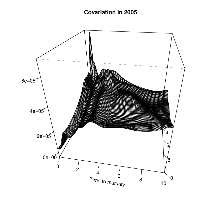
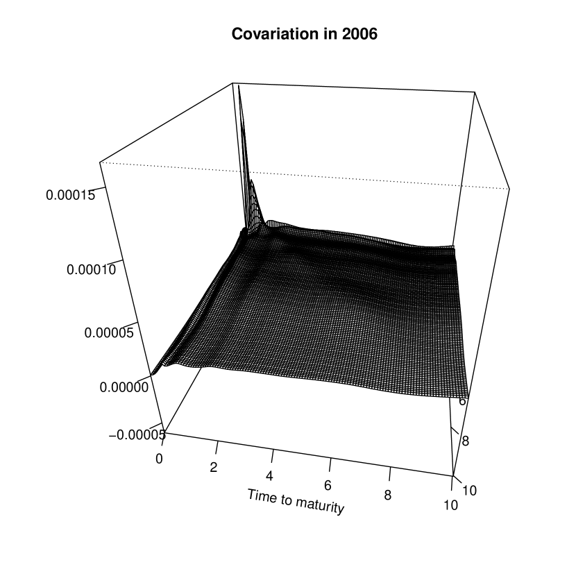
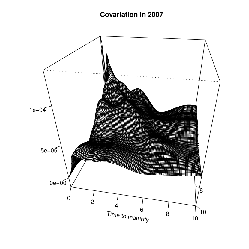
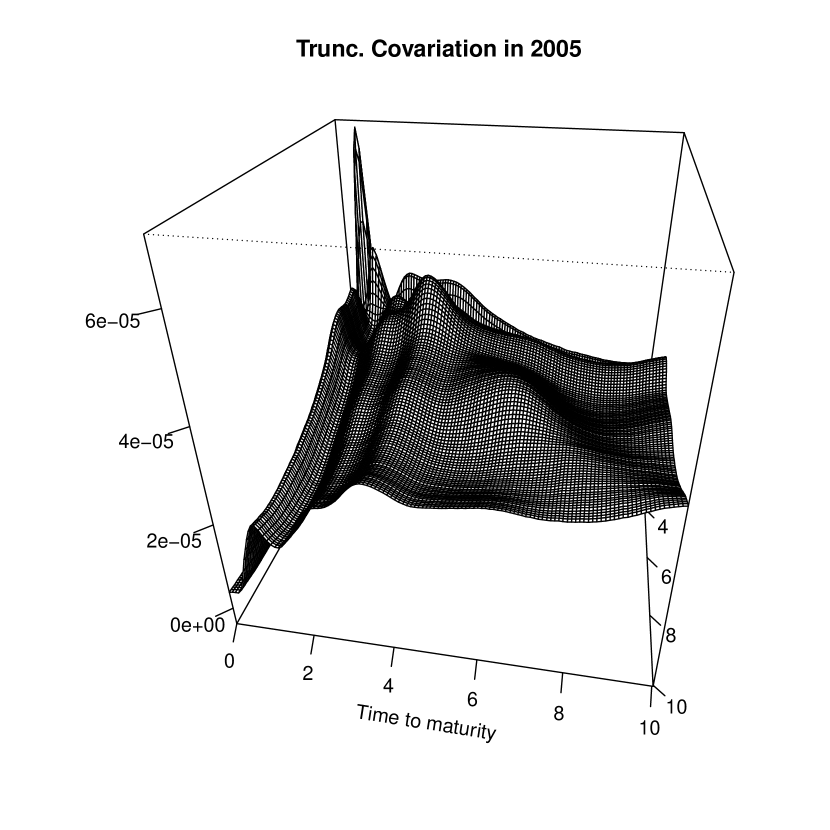
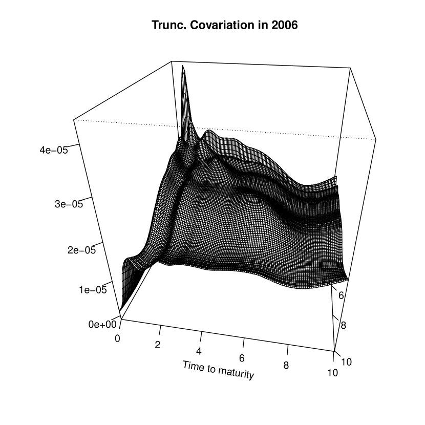
On one hand, jumps that have a moderate impact on the magnitude of the overall quadratic covariation can visually distort the shape of the volatility. Figure 1 depicts plots of the graphs of the estimated truncated kernels $q_{i}^{*,-}$ (with the truncation level $l=3$) and nontruncated kernels $q^{*}_{i}$ for the years 2005, 2006 and 2007. In 2006, which is also a year in which the yield curve inverted before the financial crisis in 2007, two jumps had a visible impact on the shape of the measured quadratic covariation kernels although they together accounted for less than 3 % of the magnitude of the quadratic covariation. This is due to a higher emphasis on the variation in difference returns with short maturities where one should note the different scalings in the plots. Removing these two jumps leads to a more time-homogeneous shape of the integrated volatility surfaces in the sense of the relation of the variation in the shorter maturities to the variation in higher maturities. On the other hand, jumps influence the magnitude of the quadratic variation. For instance, nine increments in the year 2020 (Covid-19 outbreak) sorted out by the truncation rule for $l=3$ accounted for more than 50% of the overall quadratic variation in the data as measured by its norm. The statistics for jumps in all years can be found in the supplment to this article. Interestingly, our measurements suggest that jumps tend to cluster.

Refer to caption
Refer to caption
Refer to caption
Refer to caption
Refer to caption
Refer to caption
Figure 1. The upper row shows the graphs of the estimators $q_{i}^{*}$ for the years 2006, 2007, and 2008 ($i=17,18,19$) and the lower row their truncated counterparts $q_{i}^{*,-}$ at a truncation level of $l=3$.

5.2. Dimensionality of the continuous part of the quadratic variations

We now examine the statistically relevant number of random processes that are driving the continuous part of the forward curve dynamics by investigating the dimensionality of the continuous quadratic covariation of the latent driving semimartingale via the estimator $\mathcal{T}_{\hat{q}_{i}^{*,-}}$.

Table 2 reports the number of eigenfunctions of $\mathcal{T}_{\hat{q}_{i}^{*,-}}$ that are needed to explain resp. $85\%$, $90\%$, $95\%$, and $99\%$ of the continuous covariation in the years 2005, 2006 and 2007 showing that to explain 99% of the variation at least 10 factors are needed in each year. The situation looks similar for all other years from 1990-2022, while the detailed results were relegated to the appendix. We find that the complexity of the covariation seems to have decreased over the years, indicating a time-varying pattern of the volatility term structure that goes beyond its overall level. It is noteworthy that in almost every year (30 out of 33), the number of linear factors needed to explain at least 99% of the truncated variation of the data is at least $10$. These dimensions even increase if we employ the static factors $(e_{j}^{long})_{j\in\mathbb{N}}$ of eigenvectors of $\mathcal{T}_{\hat{q}_{long}^{*}}$ and do not update them in each year. In that case, in 27 out of 33 years at least 12 factors are needed to explain at least $99\%$ of the variation in each year.

5.3. Importance of higher-order factors for short term trading strategies

A natural question is if the higher-order factors indicated by the analysis of real bond market data in Section 5 are of economic significance beyond capturing variation in difference returns. Therefore, we investigate whether the high dimensionality of the continuous quadratic varitations indicated by the estimators $\hat{q}_{i}^{*}$ and $q^{*}_{long}$ are important for other short term trading strategies than difference returns. Precisely, Define the daily return $(d_{L})_{i}^{n}(j)$ of the trading strategy of buying an $(j+L)\Delta_{n}$ bond and shorting an $j\Delta_{n}$ bond

$$(d_{L})_{i}^{n}(j):=\sum_{l=0}^{L}d_{i}^{n}(j+l)=\tilde{\Delta}^{n}_{i\Delta_{n}}\log P((j+L)\Delta_{n})-\tilde{\Delta}_{i\Delta_{n}}^{n}\log P(j\Delta_{n})$$

where $\tilde{\Delta}_{t}^{n}\log P(x)=\log P_{t+\Delta_{n}}(x)-\log P_{t+\Delta_{n}}(x-\Delta_{n})$. Evidently, we can derive them as linear functionals of either log bond price returns or difference returns.

We want to determine the adequacy of approximation of these higher-order difference returns when they are derived either from approximated log price curves, which are projected onto its leading principal components or when they are derived from difference returns, which are projected onto the leading eigencomponents of the long-term volatility estimator. For that, we calculate the relative mean absolute error ($RMAE$) for a set $\mathcal{V}=\{i_{1}\Delta_{n}^{val},...,i_{825}^{val}\Delta_{n}\}$ of dates (where in each year from 1990 to 2022 we randomly draw 25 dates making a total of 825 validation dates). That is, defining the piecewise constant kernels $(\tilde{d}_{L})_{i}^{n}=\sum_{j=1}^{\lfloor M/\Delta_{n}\rfloor}(d_{L})_{i}(j)\mathbb{I}_{[j\Delta_{n},j\Delta_{n})}$ we calculate

$$RMAE_{L}(f_{1},...,f_{d}):=\frac{1}{825}\sum_{l=1}^{825}\frac{\left\|(\tilde{d}_{L})_{i_{l}}^{n}-\mathcal{P}_{f_{1},...,f_{d}}(\tilde{d}_{L})_{i_{l}}^{n}\right\|_{L^{2}(0,10)}}{\left\|(\tilde{d}_{L})_{i_{l}}^{n}\right\|_{L^{2}(0,10)}}.$$

where $\mathcal{P}_{f_{1},...,f_{d}}:=\sum_{i=1}^{d}f_{i}^{\otimes 2}$. The factors are derived in two different ways. In the first scenario (S1), the factors $f_{1},...,f_{d}$ correspond to principal components of the empirical covariance of log-price differences $\tilde{\Delta}\log P_{i\Delta_{n}}$ for $i\notin\mathcal{V}$ and in the second scenario (S2) the factors $f_{1},...,f_{d}$ correspond to the leading eigenfunctions of the estimated stationary volatility kernel $\hat{q}_{long}^{*}$ where as before the truncation of jumps is conductcted yearwise with truncation level $l=3$ according to the truncation procedure described in Section 3.4.1.

We compare the results for lags of 7, 30, 90 and 180 days, since they approximately correspond to the returns of buying a bond and shorting another bond with time to maturity that is resp. a week, a month, a quarter or half a year higher. The $RMAE$s can be found in Table 3.

Table 3. The table shows the $RMAE$s for different numbers of factors lags and for the two different ways (S1 and S2) in which the factors are derived. In bold are errors for which 99% of the variation in difference returns resp. the log-bond prices were explained.
Lag Scenario $d$
$1$ $2$ $3$ $4$ $5$ $6$ $7$ $8$ $9$ $10$ 11 12 13 14 15 16
$Lag=7$ S1 $0.63$ ${\bf 0.50}$ $0.44$ $0.40$ $0.36$ $0.32$ $0.30$ $0.27$ $0.25$ $0.23$ $0.21$ $0.19$ $0.17$ $0.16$ $0.14$ $0.13$
S2 $0.62$ $0.50$ $0.45$ $0.40$ $0.35$ $0.32$ $0.28$ $0.25$ $0.23$ $0.20$ $0.17$ $0.15$ $0.12$ ${\bf 0.10}$ $0.09$ $0.07$
$Lag=30$ S1 $0.63$ ${\bf 0.50}$ $0.44$ $0.40$ $0.35$ $0.32$ $0.29$ $0.27$ $0.24$ $0.22$ $0.20$ $0.18$ $0.17$ $0.15$ $0.14$ $0.12$
S2 $0.62$ $0.50$ $0.45$ $0.40$ $0.35$ $0.31$ $0.28$ $0.25$ $0.22$ $0.20$ $0.17$ $0.15$ $0.12$ ${\bf 0.10}$ $0.08$ $0.07$
$Lag=90$ S1 $0.62$ ${\bf 0.49}$ $0.43$ $0.38$ $0.34$ $0.30$ $0.27$ $0.25$ $0.22$ $0.20$ $0.17$ $0.15$ $0.17$ $0.14$ $0.12$ $0.12$
S2 $0.61$ $0.49$ $0.43$ $0.38$ $0.33$ $0.29$ $0.26$ $0.23$ $0.19$ $0.17$ $0.16$ $0.13$ $0.11$ ${\bf 0.09}$ $0.07$ $0.06$
$Lag=180$ S1 $0.61$ ${\bf 0.47}$ $0.41$ $0.36$ $0.31$ $0.27$ $0.24$ $0.21$ $0.18$ $0.15$ $0.13$ $0.11$ $0.09$ $0.07$ $0.06$ $0.05$
S2 $0.60$ $0.47$ $0.41$ $0.35$ $0.30$ $0.26$ $0.22$ $0.19$ $0.15$ $0.13$ $0.13$ $0.10$ $0.08$ ${\bf 0.07}$ $0.06$ $0.05$

It can be observed that a high number of factors is needed to approximate the lagged difference returns precisely and that approximations based on low factor structures as indicated by the covariance of difference returns imply high approximation errors. While it is not surprising that the approximation gets better if we use more factors, the high discrepancy of the approximation errors is noteworthy. The errors for a typically chosen three factor model based on log price differences (the factors correspond to level, slope and curvature), which explain more than 99,7% of the variation in log-price returns is for all lags higher than $0.4$, whereas for the approximation error for 14 factors, which we would need to explain 99% of the variation in difference returns as measured by $\hat{q}_{long}^{*}$ is never higher than $0.11$. Interestingly, for all lags, choosing the factors equal to the leading eigenfunctions of the long term volatility $\hat{q}_{long}^{*}$ instead of the ones indicated by log-price differences can reduce the error for the higher-order approximations quite significantly and for $d=16$ and for lags not higher than 90 days by almost 50 %. Higher-order factors of volatility can, thus, not easily be ignored and might carry important economic information.

5.4. Concluding remarks on the empirical study

We conclude that the reported dimensions are overall quite high compared to the few factors needed to explain a large amount of the variation in yield and discount curves. This suggests that low-dimensional factor models are not able to capture all statistically relevant codependencies of bond prices. Still, exact magnitudes of explained variations of the higher order components have to be interpreted cautiously and conditional on the smoothing technique that was employed to derive yield or discount curves. However, higher-order factors seem to be economically relevant for capturing variations in short term trading strategies as indicated by the out-of-sample study of Section 5.3.

Underestimation of the number of statistically relevant random drivers can have undesirable effects. For instance, [15] showcase the potential economic impact on mean-variance optimal portfolio choices and hedging errors. At the same time, not every model that is parsimonious in its parameters needs to entail a low-dimensional factor structure such as the simple volatility model of Section 4. It seems desirable to derive parsimonious models that match the empirical observation of high or infinite-dimensional covariations and reflect the characteristics of their dynamic evolution.

Acknowledgements

I would like to thank Dominik Liebl, Fred Espen Benth, Alois Kneip and Andreas Petersson for helpful comments and discussions. Funding by the Argelander program of the University of Bonn is gratefully acknowledged.

References

  • [1] O. E. Barndorff-Nielsen, Fred Espen Benth, and Almut E. D. Veraart. Modelling energy spot prices by volatility modulated Lévy-driven Volterra processes. Bernoulli, 19(3):803 – 845, 2013.
  • [2] M. Bennedsen. A rough multi-factor model of electricity spot prices. Energy Econ., 63:301–313, 2017.
  • [3] F. Benth, G. Lord, and A. Petersson. The heat modulated infinite dimensional Heston model and its numerical approximation. Available at ArXiv:2206.10166, 2022.
  • [4] Fred Espen Benth, Barbara Rüdiger, and Andre Süss. Ornstein–Uhlenbeck processes in Hilbert space with non-Gaussian stochastic volatility. Stoch. Proc. Applic., 128(2):461–486, 2018.
  • [5] Fred Espen Benth, Dennis Schroers, and A. E. D. Veraart. A feasible central limit theorem for realised covariation of spdes in the context of functional data. Ann. Appl. Probab., 34(2):2208–2242, 2024.
  • [6] Fred Espen Benth, Dennis Schroers, and Almut E.D. Veraart. A weak law of large numbers for realised covariation in a Hilbert space setting. Stoch. Proc. Applic., 145:241–268, 2022.
  • [7] Fred Espen Benth and Carlo Sgarra. A Barndorff-Nielsen and Shephard model with leverage in Hilbert space for commodity forward markets. Available at SSRN 3835053, 2021.
  • [8] Fred Espen Benth and Iben Cathrine Simonsen. The Heston stochastic volatility model in Hilbert space. Stoch. Analysis Applic., 36(4):733–750, 2018.
  • [9] T. Björk and B. Christensen. Interest rate dynamics and consistent forward rate curves. Math. Finance, 9(4):323–348, 1999.
  • [10] T. Björk, G. Di Masi, Y. Kabanov, and W. Runggaldier. Towards a general theory of bond markets. Finance Stoch., 1:141–174, 1997.
  • [11] T. Björk and L. Svensson. On the existence of finite-dimensional realizations for nonlinear forward rate models. Math. Finance, 11(2):205–243, 2001.
  • [12] S. Cox, C. Cuchiero, and A. Khedher. Infinite-dimensional Wishart-processes. arXiv preprint arXiv:2304.03490, 2023.
  • [13] S. Cox, S. Karbach, and A. Khedher. An infinite-dimensional affine stochastic volatility model. Math. Finance, 2021.
  • [14] S. Cox, S. Karbach, and A. Khedher. Affine pure-jump processes on positive Hilbert-Schmidt operators. Stoch. Proc. Applic., 151:191–229, 2022.
  • [15] R. K. Crump and N. Gospodinov. On the factor structure of bond returns. Econometrica, 90(1):295–314, 2022.
  • [16] Giuseppe Da Prato and Jerzy Zabczyk. Stochastic Equations in Infinite Dimensions, volume 152 of Encyclopedia of Mathematics and its Applications. Cambridge University Press, Cambridge, second edition, 2014.
  • [17] D. Duffie, D. Filipović, and W. Schachermayer. Affine processes and applications in finance. Ann. Appl. Probab., 13(3):984 – 1053, 2003.
  • [18] B. Fárkas, M. Friesen, B. Rüdiger, and D. Schroers. On a class of stochastic partial differential equations with multiple invariant measures. NoDEA, 28, 2020.
  • [19] D. Filipović. A note on the Nelson–Siegel family. Math. finance, 9(4):349–359, 1999.
  • [20] D. Filipović. Exponential-polynomial families and the term structure of interest rates. Bernoulli, pages 1081–1107, 2000.
  • [21] D. Filipović. Consistency Problems for HJM Interest Rate Models, volume 1760 of Lecture Notes in Mathematics. Springer, Berlin, 2001.
  • [22] D. Filipović, M. Pelger, and Y. Ye. Stripping the discount curve - a robust machine learning approach. Swiss Finance Institute Research Paper, 2022.
  • [23] D. Filipović, S. Tappe, and J. Teichmann. Jump-diffusions in Hilbert spaces: existence, stability and numerics. Stochastics, 82(5):475–520, 2010.
  • [24] D. Filipović and J. Teichmann. Existence of invariant manifolds for stochastic equations in infinite dimension. J. Funct. Anal., 197(2):398–432, 2003.
  • [25] M. Friesen and S. Karbach. Stationary covariance regime for affine stochastic covariance models in hilbert spaces. arXiv preprint arXiv:2203.14750, 2022.
  • [26] D. Heath, R. Jarrow, and A. Morton. Bond pricing and the term structure of interest rates: A new methodology for contingent claims valuation. Econometrica, 60(1):77–105, 1992.
  • [27] J. Jacod. Asymptotic properties of realized power variations and related functionals of semimartingales. Stoch. Proc. Applic., 118(4):517–559, 2008.
  • [28] J. Jacod and P. Protter. Discretization of Processes, volume 67 of Stochastic Modelling and Applied Probability. Springer, Heidelberg, 2012.
  • [29] O. Linton, E. Mammen, J.P. Nielsen, and C. Tanggaard. Yield curve estimation by kernel smoothing methods. J. Econ., 105(1):185–223, 2001.
  • [30] R. Litterman and J. Scheinkman. Common factors affecting bond returns. J. Fixed Income, 1:62–74, 1991.
  • [31] Y. Liu and C. Wu. Reconstructing the yield curve. J. financ. econ., 142(3):1395–1425, 2021.
  • [32] C. Mancini. Disentangling the jumps of the diffusion in a geometric jumping brownian motion. Giornale dell’Istituto Italiano degli Attuari, 64:19–47, 2001.
  • [33] C. Mancini. Estimating the integrated volatility in stochastic volatility models with lévy type jumps. Tech. rep., Università di Firenze, 2004.
  • [34] C. Mancini. Nonparametric threshold estimation for models with stochastic diffusion coefficient and jumps. Scand. J. Statist., 36:270–296, 2009.
  • [35] C. Mancini and F. Calvori. Jumps, chapter Seventeen, pages 403–445. John Wiley & Sons, Ltd, 2012.
  • [36] V. Mandrekar and B. Rüdiger. Stochastic integration in Banach spaces, volume 73 of Probability Theory and Stochastic Modelling. Springer, 2015.
  • [37] C. Marinelli. Well-posedness and invariant measures for hjm models with deterministic volatility and lévy noise. Quant. Finance, 10(1):39–47, 2010.
  • [38] V. Masarotto, V. M. Panaretos, and Y. Zemel. Procrustes metrics on covariance operators and optimal transportation of gaussian processes. Sankhya A, 81(1):172–213, 2019.
  • [39] S. Peszat and J. Zabczyk. Stochastic Partial Differential Equations with Lévy Noise, volume 113 of Encyclopedia of Mathematics and its Applications. Cambridge University Press, Cambridge, 2007.
  • [40] M. Piazzesi. Affine term structure models. In Handbook of financial econometrics: Tools and Techniques, pages 691–766. Elsevier, 2010.
  • [41] James Ramsay and B. W. Silverman. Functional Data Analysis. Springer Series in Statistics. Springer, second edition, 2005.
  • [42] H. Ren, N. Chen, and C. Zou. Projection-based outlier detection in functional data. Biometrika, 104(2):411–423, 2017.
  • [43] A. Rusinek. Mean reversion for hjmm forward rate models. Adv. in Appl. Probab., 42(2):371–391, 2010.
  • [44] D. Schroers. Robust functional data analysis for stochastic evolution equations in infinite dimensions. arXiv preprint, 2024.
  • [45] M. Tehranchi. A Note on Invariant Measures for HJM Models. Finance Stoch., 9(3):389–398, 2005.
  • [46] T. Vargiolu. Invariant measures for the Musiela equation with deterministic diffusion term. Finance Stoch., 3(4):483–492, 1999.
  • [47] J. Zhang and J. Chen. Statistical inferences for functional data. Ann. Statist., 35(3):1052 – 1079, 2007.

Appendix A Itô semimartingales in Hilbert spaces

In this appendix, we provide an introduction and technical details for the class of Itô semimartingales that we consider throughout the paper.

First, we specify the components of the driver $X$ which is an $L^{2}(\mathbb{R}_{+})$-valued right-continuous process with left-limits (càdlàg) that can be decomposed as

$$X_{t}:=X_{t}^{C}+J_{t}:=(A_{t}+M_{t}^{C})+J_{t}\quad t\geq 0.$$

Here, $A$ is a continuous process of finite variation, $M^{C}$ is a continuous martingale and $J$ is another martingale modeling the jumps of $X$. We assume that $X$ is an Itô semimartingale for which the components have integral representations

(19) $$A_{t}:=\int_{0}^{t}\alpha_{s}ds,\quad M_{t}^{C}:=\int_{0}^{t}\sigma_{s}dW_{s},\quad J_{t}:=\int_{0}^{t}\int_{H\setminus\{0\}}\gamma_{s}(z)(N-\nu)(dz,ds).$$

For the first part $(\alpha_{t})_{t\geq 0}$ is an $H$-valued and and almost surely integrable (w.r.t. $\|\cdot\|_{L^{2}(\mathbb{R}_{+})}$) process that is adapted to the filtration $(\mathcal{F}_{t})_{t\geq 0}$.

The volatility process $(\sigma_{t})_{t\geq 0}$ is predictable and takes values in the space of Hilbert-Schmidt operators $L_{\text{HS}}(U,L^{2}(\mathbb{R}_{+}))$ from a separable Hilbert space $U$ into $L^{2}(\mathbb{R}_{+})$. Moreover, we have $\mathbb{P}[\int_{0}^{T}\|\sigma_{s}\|_{\text{HS}}^{2}ds<\infty]=1$. The space $U$ is left unspecified, as it is just formally the space on which the Wiener process $W$ is defined and does not affect the distribution of $X$. The cylindrical Wiener process $W$ is a weakly defined Gaussian process with independent stationary increments and covariance $I_{U}$, the identity on $U$. One might consult the standard textbooks [16], [36] or [39] for the integration theory w.r.t. $W$.

For the jump process $J$, we define a homogeneous Poisson random measure $N$ on $\mathbb{R}_{+}\times H\setminus\{0\}$ and its compensator measure $\nu$ which is of the form $\nu(dz,dt)=F(dz)\otimes dt$ for a $\sigma$-finite measure $F$ on $\mathcal{B}(H\setminus\{0\})$. The process $\gamma_{s}(z))_{s\geq 0,z\in H\setminus\{0\}}$ is the $l^{2}(\mathbb{R}_{+})$-valued jump volatility process and is predictable and stochastically integrable w.r.t. the compensated Poisson random measure $\tilde{N}:=(N-\nu)$. For a detailed account on stochastic integration w.r.t. compensated Poisson random measures in Hilbert spaces, we refer to [36] or [39].

Let us now rewrite the quadratic covariation (4) of $X$ in terms of the volatility $\sigma$ and the jumps of the process as

(20) $\displaystyle[X,X]_{t}=[X^{C},X^{C}]_{t}+[J,J]_{t}=\int_{0}^{t}\Sigma_{s}ds+\sum_{s\leq t}(X_{s}-X_{s-})^{\otimes 2},$

where $\Sigma_{s}=\sigma_{s}\sigma_{s}^{*}$ (where $\sigma_{s}^{*}$ is the Hilbert space adjoint) and $X_{t-}:=\lim_{s\uparrow t}X_{s}$ is the left limit of $(X_{t})_{t\geq 0}$ at $t$, which is well-defined, since $X_{t}$ has càdlàg paths. This characterization follows as a special case of Theorem 3.1 in [44]

Let us now reconsider Example 2.2.

Example A.1 (Rewriting an $L^{2}(\mathbb{R}_{+})$-valued Poisson random measure in compensated form).

In Example 2.2 it was remarked that a compound Poisson process $J_{t}=\sum_{i=1}^{N_{t}}\chi_{i}$ is strictly speaking not a valid choice for the jump process, since it is not a martingale. Here we show that the semimartingale in the example can be easily rewritten to have the desired form: For that, define the Poisson random measure $N(B,[0,t]):=\#\{i\leq N_{t}:\chi_{i}\in B\}$ for $B\in\mathcal{B}(H\setminus\{0\}),t\geq 0.$ This has compensator measure $\nu=\lambda dt\otimes F(dz)$, so we can redefine $J$ in a formally correct manner by $J_{t}=\sum_{i=1}^{N_{t}}\chi_{i}-\lambda t\mathbb{E}[\chi_{1}]=\int_{0}^{t}\int_{L^{2}(\mathbb{R}_{+})\setminus\{0\}}z(N-\nu)(dz,ds)$ and set $A_{t}=(a+\lambda\mathbb{E}[X_{1}])t$.

Appendix B Technical Assumptions

This section contains the technical Assumptions that are needed for the validity of Theorems 3.1, 3.3, 3.6, 3.8 and 3.10.

B.1. Assumption for derivation of idenifiability of $[X^{C},X^{C}]$ and $[J,J]$

To derive asymptotic results for $\hat{q}^{n,-}_{t}$ in Theorem 3.3, we introduce

Assumption B.1 (r).

$\alpha$ is locally bounded, $\sigma$ is càdlàg and there is a localizing sequence of stopping times $(\tau_{n})_{n\in\mathbb{N}}$ and for each $n\in\mathbb{N}$ a real valued function $\Gamma_{n}:H\setminus\{0\}\to\mathbb{R}$ such that $\|\gamma_{t}(z)(\omega)\|\wedge 1\leq\Gamma_{n}(z)$ whenever $t\leq\tau_{n}(\omega)$ and $\int_{L^{2}(\mathbb{R}_{+})\setminus\{0\}}\Gamma_{n}(z)^{r}F(dz)<\infty$.

Assumption B.1 used in Theorem 3.3 is a direct generalization of Assumption (H-r) in [28]. It implies that for $r<2$, the jumps of the process are $r$-summable, that is, we have

$$\sum_{s\leq t}\|X_{s}-X_{s-}\|^{l}<\infty\quad\forall l>r.$$

B.2. Assumption for derivation of convergence rates

For the derivation of convergence rates in Theorem 3.6, observe that, since $\Sigma_{t}=\sigma_{t}\sigma_{t}^{*}$ is for each $t\geq 0$ a Hilbert-Schmidt operator, we can find a process of kernels

(21) $$q_{t}^{C},\text{ such that }\Sigma_{t}=\mathcal{T}_{q_{t}^{C}}\quad\forall t\geq 0.$$

It is seems natural to impose Hölder-regularity assumptions on the volatility kernel $q_{t}^{C}$ for $t\geq 0$ to derive the error bounds. For instance, one might consider a Hölder continuous volatility kernel, such that $q_{t}^{C}\in C^{\gamma}(\mathbb{R}_{+}^{2})$ for

$$C^{\gamma}(\mathbb{R}_{+}^{2}):=\left\{q:\mathbb{R}_{+}^{2}\to\mathbb{R}:\sup_{x,y,x^{\prime},y^{\prime}\leq M}\frac{|q(x,y)-q(x^{\prime},y^{\prime})|}{\|(x,y)-(x^{\prime},y^{\prime})\|_{\mathbb{R}^{2}}^{\gamma}}<\infty\quad\forall M\geq 0\right\}.$$

However, we can consider weaker regularity conditions, which do not necessarily assume the kernels to be continuous. Namely, we require $q_{t}^{C}\in\mathfrak{F}_{\gamma}$ where

$\displaystyle\mathfrak{F}_{\gamma}:=$ $\displaystyle\left\{q\in L^{2}(\mathbb{R}_{+}^{2}):\|q\|^{2}_{\mathfrak{F}_{\gamma}(\mathbb{R}_{+}^{2})}:=\sup_{r>0}\int_{\mathbb{R}_{+}^{2}}\frac{(q(r+x,y)-q(x,y))^{2}}{r^{2\gamma}}dxdy<\infty\right\}.$

The classes $\mathfrak{F}_{\gamma}$ might appear abstract but, in particular, it contains Hölder spaces, that is,

(22) $$C^{\gamma}(\mathbb{R}_{+}^{2})\subset\mathfrak{F}_{\gamma}.$$

Vice versa, $\mathfrak{F}_{\gamma}$ is not a subset of $C^{\gamma}$ but it is strictly larger, allowing for discontinuities in volatility kernels: Let $g(x,y):=\mathbb{I}_{[a,b]}(x)\mathbb{I}_{[a,b]}(y)$ for an interval $[a,b]\subset\mathbb{R}_{+}$. Then clearly, $g$ is not an element of $C^{\frac{1}{2}}(\mathbb{R}_{+}^{2})$ as it is discontinuous. However, it is $\|g\|_{\mathfrak{F}_{1/2}}=2(b-a)<\infty.$ Hence $g\in\mathfrak{F}_{1/2}$, while $g\notin\mathfrak{F}_{\rho}$ for any $\rho>1/2$.

We now state our formal regularity assumption.

Assumption B.2.

[$\gamma$] Let $\gamma\in(0,1/2]$. We have $q^{C}_{t}\in\mathfrak{F}_{\gamma}$ $\mathbb{P}\otimes dt$-almost everywhere and

(23) $$\mathbb{P}\left[\int_{0}^{T}\|q_{s}^{C}\|_{\mathfrak{F}_{\gamma}}ds<\infty\right]=1,\quad T>0.$$
Remark B.3.

Regularity Assumption B.2 is sharp in Theorem 3.6 in the sense that for every $\gamma^{\prime}<\gamma$ we can always specify a squared volatility process $(\Sigma_{t})_{t\geq 0}$ such that in probability $\Delta_{n}^{-\gamma}\sup_{t\in[0,T]}\left\|\mathcal{T}_{\hat{q}^{n,-}_{t}}-[X^{C},X^{C}]\right\|_{\text{HS}}$ diverges but the process of kernels $(q_{t}^{C})_{t\geq 0}$ fulfills Assumption B.2 for $\gamma^{\prime}$ and (and not for $\gamma$) (c.f. Example 3.6 in [5]).

As a result of Theorem 3.6 and (22), we can derive rates of convergence also under Hölder regularity assumptions.

Corollary B.4.

If Assumption B.1(r) holds for some $r\in(0,2)$ and for all $t\geq 0$ it is $q_{t}\in C^{\gamma}(\mathbb{R}_{+}^{2})$ $\mathbb{P}\otimes dt$-almost everywhere for some $\gamma\in(0,1/2]$, then (15) holds for all $\rho<(2-r)w$ and (16) holds if $r<2(1-\gamma)$ and $w\in[\gamma/(2-r),1/2]$.

For the central limit theorem, we further need

Assumption B.5.

It is almost surely

(24) $$\int_{0}^{T}\sup_{r\geq 0}\frac{\|(I-\mathcal{S}(r))\sigma_{s}\|_{\text{op}}^{2}}{r}ds<\infty,\quad T>0.$$

B.3. Assumptions for Long-time estimators

We introduce

Assumption B.6.

The process $(\Sigma_{t})_{t\geq 0}$ is mean stationary and mean ergodic, in the sense that $\mathbb{E}\left[\|\sigma_{s}\|^{2}_{L_{\text{HS}}(U,L^{2}(\mathbb{R}_{+}))}\right]<\infty$ and there is an operator $\mathcal{C}$ such that for all $t$ it is $\mathcal{C}=\mathbb{E}[\Sigma_{t}]$ and as $T\to\infty$ we have in probability an w.r.t. the Hilbert-Schmidt norm that

(25) $$\frac{1}{T}\int_{0}^{T}\Sigma_{s}ds=\frac{[X^{C},X^{C}]_{T}}{T}\to\mathcal{C}.$$

Under Assumption B.6 we have that $\mathbb{E}[(M_{t}^{C})^{\otimes 2}]=\mathbb{E}[(\int_{0}^{t}\sigma_{s}dW_{s})^{\otimes 2}]=t\mathcal{C}\quad\forall t\geq 0.$ Hence, $\mathcal{C}$ is the covariance of the driving continuous martingale $M^{C}$ (scaled by time). Hence, as for regular functional principal component analyzes, we can find approximately a linearly optimal finite-dimensional approximation of the driving martingale, by projecting onto the eigencomponents of $\mathcal{C}$. Even more, $\mathcal{C}$ is the instantaneous covariance of the process $f$ in the sense that $\mathcal{C}=\lim_{n\to\infty}\mathbb{E}[(f_{t+\Delta_{n}}-\mathcal{S}(\Delta_{n})f_{t})^{\otimes 2}]/\Delta_{n}.$ To estimate $\mathcal{C}$, we make use of a moment assumption for the coefficients.

Assumption B.7.

[p,r] For $p,r>0$ such that $\mathbb{E}\left[\|\gamma_{s}(z)\|^{r}\right]=\Gamma(z)$ independent of $s$ for all $s\geq 0$ and there is a constant $A>0$ such that for all $s\geq 0$ it is

$$\mathbb{E}\left[\|\alpha_{s}\|_{L^{2}(\mathbb{R}_{+})}^{p}+\|\sigma_{s}\|_{\text{HS}}^{p}+\int_{L^{2}(\mathbb{R}_{+})\setminus\{0\}}\|\gamma_{s}(z)\|^{r}\nu(dz)\right]\leq A.$$

Moreover, we also make an assumption on the regularity of the volatility.

Assumption B.8.

[$\gamma$] With the notation (21) we have for $\gamma\in(0,\frac{1}{2}]$ that there is a constant $A>0$ such that for all $s\geq 0$ it is

$$\mathbb{E}\left[\|q_{s}^{C}\|_{\mathfrak{F}_{\gamma}}\right]\leq A.$$

Appendix C Proofs of section 2

Proof of the general nonsemimartingality of models in Example 2.4.

We need to prove that

(26) $\displaystyle f_{t}=f_{0}+\int_{0}^{t}k(\cdot+t-s)d\beta_{s}$

is not a continuous semimartingale where $k\in L^{2}(\mathbb{R}_{+})$, $\beta$ is a univariate standard Brownian motion. Therefore, assume that $f_{t}$ defines a semimartingale in $L^{2}(\mathbb{R}_{+})$ of the form $f_{t}=A_{t}+M_{t}$ for an $H$-valued continuous martingale $M$ and a finite variation process $A$. Observe that we also have that $f$ is a weak solution to the stochastic partial differential equation

$$\frac{d}{dx}f_{t}dt+(e\otimes k)dW_{t},\quad t\geq 0,$$

for a cylindrical Wiener process $W$ such that $\beta=\langle e,W\rangle$. Hence, for an orthonormal basis $(e_{j})_{j\in\mathbb{N}}\subset D(d/dx)$ we find that

$$\langle f_{t},e_{j}\rangle=\langle f_{0},e_{j}\rangle+\int_{0}^{t}\langle f_{s},\left(\frac{d}{dx}\right)^{*}e_{j}\rangle ds+\langle k,e_{j}\rangle\beta_{t}.$$

These are a one-dimensional semimartingales for which the first integral is of finite variation and the second part is of quadratic variation. As the decomposition of a continuous semimartingale into a continuous part with finite variation and a continuous martingale (which vanishes at 00) with quadratic variation is unique up to $\mathbb{P}\otimes dt$ nullsets, we obtain that $\mathbb{P}\otimes dt$-almost everywhere

$$\langle A_{t},e_{j}\rangle=\int_{0}^{t}\langle f_{s},\left(\frac{d}{dx}\right)^{*}e_{j}\rangle\qquad\langle M_{t},e_{j}\rangle=\langle k,e_{j}\rangle\beta_{t}\quad\forall t\geq 0,j\in\mathbb{N}.$$

Therefore, we must have $M_{t}=\beta_{t}k$ and we must have $\sum_{i=1}^{n}\Delta_{i}^{n}f^{\otimes 2}=\sum_{i=1}^{n}\Delta_{i}^{n}M_{t}^{\otimes 2}\to k^{\otimes 2}$ in probability as $n\to\infty$. Defining

$$S_{t}^{n}:=\sqrt{n}\langle f_{t},\mathbb{I}_{[0,\Delta_{n}]}\rangle,$$

we also obtain that in probability

$$\left|\sum_{i=1}^{n}(\Delta_{i}^{n}S^{n})^{2}-n\langle k,\mathbb{I}_{[0,\Delta_{n}]}\rangle^{2}\right|\leq\|\sum_{i=1}^{n}\Delta_{i}^{n}f^{\otimes 2}-k^{\otimes 2}\|_{L_{\text{HS}}(L^{2}(\mathbb{R}_{+})}\to 0$$

and since as $n\to\infty$ it is $\sqrt{n}\langle k,\mathbb{I}_{[0,\Delta_{n}]}\rangle=\Delta_{n}^{1/2+H}/(H+1)\to 0$ we also find that as $n\to\infty$ and in probability that $\sum_{i=1}^{n}(\Delta_{i}^{n}S^{n})^{2}\to 0$ must hold. Moreover, we find, since the kernel $k$ is square integrable and $k(t)=t^{H}$ on $t\in[0,1]$ that by the Burkholder-Davis-Gundy inequality for $\epsilon>0$

$\displaystyle\mathbb{E}[(\Delta_{i}^{n}S^{n})^{2+\epsilon}]^{\frac{2}{2+\epsilon}}$
$\displaystyle\leq$ $\displaystyle 2\int_{(i-1)\Delta_{n}}^{i\Delta_{n}}\|k(i\Delta_{n}+\cdot-s)\|^{2}ds$
$\displaystyle\qquad+2n\int_{0}^{(i-1)\Delta_{n}}\langle k(i\Delta_{n}+\cdot-s)-k((i-1)\Delta_{n}+\cdot-s),\mathbb{I}_{[0,\Delta_{n}]}\rangle^{2}ds$
$\displaystyle\leq$ $\displaystyle 2\|k\|^{2}\Delta_{n}+2n\int_{0}^{(i-1)\Delta_{n}}\left(\int_{0}^{\Delta_{n}}(i\Delta_{n}+y-s)^{H}-((i-1)\Delta_{n}+y-s)^{H}dy\right)^{2}ds$
$\displaystyle\leq$ $\displaystyle 2\|k\|^{2}\Delta_{n}+2n\int_{0}^{(i-1)\Delta_{n}}\frac{4}{(H+1)^{2}}\left((i\Delta_{n}-s)^{H+1}-((i-1)\Delta_{n}-s)^{H+1}\right)^{2}ds.$

Now, using the mean value theorem and since $t^{H}$ is decreasing in $t$ we find

$\displaystyle\mathbb{E}[(\Delta_{i}^{n}S^{n})^{2+\epsilon}]^{\frac{2}{2+\epsilon}}\leq$ $\displaystyle 2\|k\|^{2}\Delta_{n}+8\Delta_{n}\int_{0}^{(i-1)\Delta_{n}}((i-1)\Delta_{n}-s)^{2H}ds$
$\displaystyle\leq$ $\displaystyle 2\|k\|^{2}\Delta_{n}+8\Delta_{n}\frac{1}{2H+1}.$

This shows in particular, that by Jensen’s inequality we have

$\displaystyle\mathbb{E}\left[\left(\sum_{i=1}^{n}(\Delta_{i}^{n}S^{n})^{2}\right)^{\frac{2+\epsilon}{2}}\right]\leq$ $\displaystyle n^{\frac{2+\epsilon}{2}-1}\sum_{i=1}^{n}\mathbb{E}[(\Delta_{i}^{n}S^{n})^{2+\epsilon}]\leq\left(\|k\|^{2}+\frac{8}{2H+1}\right)^{\frac{2+\epsilon}{2}},$

which shows that $\sum_{i=1}^{n}(\Delta_{i}^{n}S^{n})^{2}$ is uniformly integrable. Thus, convergence in probability must imply convergence of the mean and we must have

$$\mathbb{E}[\sum_{i=1}^{n}(\Delta_{i}^{n}S^{n})^{2}]\to 0\quad\text{ as }n\to\infty.$$

However, we can show similarly to the calculations before that using the mean value theorem it is

$\displaystyle\mathbb{E}\left[\sum_{i=1}^{n}(\Delta_{i}^{n}S^{n})^{2}\right]\geq$ $\displaystyle n\int_{0}^{(i-1)\Delta_{n}}\langle k(i\Delta_{n}+\cdot-s)-k((i-1)\Delta_{n}+\cdot-s),\mathbb{I}_{[0,\Delta_{n}]}\rangle^{2}ds$
$\displaystyle\geq$ $\displaystyle 4\Delta_{n}\int_{0}^{(i-1)\Delta_{n}}((1+i)\Delta_{n}-s)^{2H})ds$
$\displaystyle=$ $\displaystyle\frac{4}{2H+1}\Delta_{n}^{2H+2}((1+i)^{2H+1}-2^{2H+1}).$

Thus, writing $K=4/(2H+1)H^{2}(H+1)^{2}$ we find

$$\mathbb{E}[\sum_{i=1}^{n}(\Delta_{i}^{n}S^{n})^{2}]\geq K\Delta_{n}^{2H+2}\sum_{i=1}^{n}(1+i)^{2H+1}-K\Delta_{n}^{2H+2}\sum_{i=1}^{n}2^{2H+1}.$$

While the second term is $o(1)$, for the first term it is

$$K\Delta_{n}^{2H+2}\sum_{i=1}^{n}(1+i)^{2H+1}\geq K\Delta_{n}^{2H+2}\int_{0}^{n+1}x^{2H+1}dx=\frac{K}{2H+2}\left(\frac{n+1}{n}\right)^{2H+2}\geq\frac{K}{2H+2}.$$

This cannot hold, since by the uniform integrability of the sequence $\sum_{i=1}^{n}(\Delta_{i}^{n}S^{n})^{2}$ we have that the mean $\mathbb{E}[\sum_{i=1}^{n}(\Delta_{i}^{n}S^{n})^{2}]$ must converge to 00. ∎

Appendix D Proofs of Section 3

In this Section we prove the results of Section 3. For that, we first prove an abstract limit theory for general evolution equations in Section D.1. We then derive the results of Section 3 using this abstract result in Section D.2

D.1. An Abstract limit theorem

The asymptotic theory elaborated in the article follows by an abstract result for abstract evolution equations in Hilbert spaces, which we present and prove in this section. Roughly speaking, we prove that the results in [44] are valid, also when we discretized the functional data also in the cross-section in a particular manner, that we will make precise next. For now let $f$ be a mild solution to a stochastic evolution equation of the for described in (6).

We also introduce the notation

$$H:=L^{2}(\mathbb{R}_{+}).$$

We do this, because the subsequent Theorem D.1 holds under much more general conditions than for the term structure setting and with this notation it becomes simple to appreciate this generality. That is, Theorem D.1 holds for general separable Hilbert spaces $H$, semigroups $\mathcal{S}$ and general $H$-valued Itô semimartingale as described in [44]. To be consistent with the notation and since we do not want to restate all Assumptions for the abstract case, (they can be found in [44] we formally chose to state the theorem and its proofs for the term structure setting only.

For the cross-sectional discretization we introduce a sequence of projections $(\Pi_{m})_{m\in\mathbb{N}}$ that coverges strongly to a projection operator $\Pi:H\to H$, which is not necessarily the identity. In the case of term structure models, $\Pi_{m}$ is defined as in (11) for which $\Pi f(x)=f(x)\mathbb{I}_{[0,M]}(x)$. We define the discretized truncated semigroup-adjusted realized covariation as

(27) $$SARCV_{t}^{n}(u_{n},-,m):=\sum_{i=1}^{\lfloor t/\Delta_{n}\rfloor}\Pi_{m}\tilde{\Delta}_{i}^{n}f^{\otimes 2}\mathbb{I}_{g_{n}(\Pi_{m}\tilde{\Delta}_{i}^{n}f)\leq u_{n}}$$

for $m,n\in\mathbb{N}\cup\{\infty\}$ and a sequence $(u_{n})_{n\in\mathbb{N}}\subset\mathbb{R}\cup\{\infty\}$ and a sequence of truncation functions $g_{n}:L^{2}(\mathbb{R}_{+})\to\mathbb{R}_{+}$, such that there are constants $c,C>0$ such that for all $f\in H$ we have

(28) $\displaystyle c\|f\|_{H}\leq g_{n}(f)\leq C\|f\|_{H},\quad g_{n}(f+h)\leq g_{n}(h)+g_{n}(f)$

Observe that if $\Pi=I$ is the identity on $H$, it is $SARCV(u_{n},-,\infty)=SARCV(u_{n},-)$ as in the previous section. As a consequence of the possibile noncommutativity of the semigroup and the projections $\Pi_{m}$, the rates of convergence also depends on

(29) $$b_{m}^{T}:=\int_{0}^{T}\|\Pi\Sigma\Pi-\Pi_{m}\Sigma_{s}\Pi_{m}\|_{\text{HS}}ds.$$

Here we again use the notation $\Sigma_{t}=\sigma_{t}\sigma_{t}^{*}$ for $t\geq 0$. That $b_{m}^{T}$ indeed converges to 00 almost surely as $m\to\infty$ is a Corollary of Proposition 4 and Lemma 5 in [38].

Theorem D.1.
  • (i)

    As $n,m\to\infty$ and w.r.t. the Hilbert-Schmidt norm it is

    $$SARCV_{t}^{n}(\infty,-,m)\overset{u.c.p.}{\longrightarrow}\Pi[X,X]_{t}\Pi=\int_{0}^{t}\Pi\Sigma_{s}\Pi ds+\sum_{s\leq t}\left(\Pi X_{s}-\Pi X_{s-}\right)^{\otimes 2}.$$
  • (ii)

    Under Assumption B.1(2) and w.r.t. the Hilbert-Schmidt norm and as $n,m\to\infty$ it is

    $$SARCV_{t}^{n}(u_{n},-,m)\overset{u.c.p.}{\longrightarrow}\Pi[X^{C},X^{C}]_{t}\Pi=\int_{0}^{t}\Pi\Sigma_{s}\Pi ds.$$
  • (iii)

    Let Assumptions B.1(r) hold for some $r\in(0,2)$ and Assumption B.2($\gamma$) hold for some $\gamma\in(0,1/2]$. Then it is for each $\rho<(2-r)w$, $T\geq 0$ as $n,m\to\infty$

    $$\sup_{t\in[0,T]}\left\|SARCV_{t}^{n}(u_{n},-,m)-\Pi[X^{C},X^{C}]_{t}\Pi\right\|_{text{HS}}=\mathcal{O}_{p}(\Delta_{n}^{\min(\gamma,\rho)}+b_{m}^{T})$$

    In particular, if $r<2(1-\gamma)$ and $w\in[\gamma/(2-r),1/2]$ we have

    $$\sup_{t\in[0,T]}\left\|SARCV_{t}^{n}(u_{n},-,m)-\Pi[X^{C},X^{C}]_{t}\Pi\right\|_{\text{HS}}=\mathcal{O}_{p}(\Delta_{n}^{\gamma}+b_{m}^{T})$$
  • (iv)

    Assume that

    (30) $\displaystyle\mathbb{P}\left[\int_{0}^{T}\sup_{r\geq 0}\frac{\|(I-\mathcal{S}(r))\sigma_{s}\|_{\text{op}}^{2}}{r}ds<\infty\right]=1.$

    Then Assumption B.2($1/2$) holds. Let, moreover, Assumption B.1(r) hold for $r<1$, let $w\in[1/(2-r),1/2]$ and assume that $b_{m}^{T}=o_{p}(\Delta_{n}^{\frac{1}{2}})$. Then we have w.r.t. the $\|\cdot\|_{L_{\text{HS}}(H)}$ norm and as $n,m\to\infty$ that

    $$\sqrt{n}\left(SARCV_{t}^{n}(u_{n},-,m)_{t}^{n}-\Pi[X^{C},X^{C}]_{t}\Pi\right)\overset{st.}{\longrightarrow}\Pi\mathcal{N}(0,\mathfrak{Q}_{t})\Pi,$$

    where $\mathcal{N}(0,\mathfrak{G}_{t})$ is for each $t\geq 0$ a Gaussian random variable in $L_{\text{HS}}(H)$ defined on a very good filtered extension $(\tilde{\Omega},\tilde{\mathcal{F}},\tilde{\mathcal{F}}_{t},\tilde{\mathbb{P}})$ of $(\Omega,\mathcal{F},\mathcal{F}_{t},\mathbb{P})$ with mean 00 and covariance given for each $t\geq 0$ by a linear operator $\mathfrak{Q}_{t}:L_{\text{HS}}(H)\to L_{\text{HS}}(H)$ such that

    $$\mathfrak{Q}_{t}=\int_{0}^{t}\Sigma_{s}(\cdot+\cdot^{*})\Sigma_{s}ds.$$
  • (v)

    Let Assumption B.6 hold and $\mathcal{C}=\mathbb{E}[\Sigma_{t}]$ denote the global covariance of the continuous driving martingale. Let furthermore Assumption B.7(p,r) and B.8($\gamma$) hold (for the abstract semigroup $\mathcal{S}$) for some $r\in(0,2)$, $\gamma\in(0,1/2]$ and $p>\max(2/(1-2w),(1-wr)/(2w-rw))$. Then we have w.r.t. the Hilbert-Schmidt norm that as $n,m,T\to\infty$

    $$\frac{1}{T}SARCV_{T}^{n}(u_{n},-,m)\overset{p}{\longrightarrow}\Pi\mathcal{C}\Pi.$$

    If $r<2(1-\gamma)$ and $w\in(\gamma/(1-2w),1/2)$, $p\geq 4$ and observing that $\varphi_{m}=\text{tr}((I-\Pi_{m})\mathbb{E}[\Sigma_{1}](I-\Pi_{m}))$ converges to 00 as $m\to\infty$ (where tr denotes the trace operation) we have with $a_{T}=\|[X^{C},X^{C}]/T-\mathcal{C}\|_{\text{HS}}$ that

    $$\left\|\frac{1}{T}SARCV_{T}^{n,m}(-)-\Pi\mathcal{C}\Pi\right\|_{\mathcal{H}}=\mathcal{O}_{p}(\Delta_{n}^{\gamma}+\varphi_{m}+a_{T}).$$

To prove this abstract result, we make use of the limit theory established in [44]. However, Theorem D.1 is not a direct corollary of these results, since we have to take into account that jump-truncation rules now also depend on possible discrete approximations. The key result to bridge this gap is

Lemma D.2.

Assume that Assumptions B.7(p,r) holds for $r\in(0,2]$ and $p>(1-\rho/((2-r)w))^{-1}$ for some $\rho<(2-r)w$ when $r<2$ or $\rho=0$ if $r=2$. Then we have

(31) $\displaystyle\mathbb{E}\left[\left\|\sum_{i=1}^{\lfloor t/\Delta_{n}\rfloor}(\Pi_{m}\tilde{\Delta}_{i}^{n}f)^{\otimes 2}\mathbb{I}_{g_{n}(\Pi_{m}\tilde{\Delta}_{i}^{n}f)\leq u_{n}}-\sum_{i=1}^{\lfloor t/\Delta_{n}\rfloor}(\Pi_{m}\tilde{\Delta}_{i}^{n}f)^{\otimes 2}\mathbb{I}_{g_{n}(\tilde{\Delta}_{i}^{n}f)\leq u_{n}}\right\|\right]=Kt\Delta_{n}^{\rho}\phi_{n}$

for a real sequence $(\phi_{n})_{n\in\mathbb{N}}$ converging to 00 and a constant $K>0$.

If Assumption B.1 holds, it is

(32) $\displaystyle\left\|\sum_{i=1}^{\lfloor t/\Delta_{n}\rfloor}(\Pi_{m}\tilde{\Delta}_{i}^{n}f)^{\otimes 2}\mathbb{I}_{g_{n}(\Pi_{m}\tilde{\Delta}_{i}^{n}f)\leq u_{n}}-\sum_{i=1}^{\lfloor t/\Delta_{n}\rfloor}(\Pi_{m}\tilde{\Delta}_{i}^{n}f)^{\otimes 2}\mathbb{I}_{g_{n}(\tilde{\Delta}_{i}^{n}f)\leq u_{n}}\right\|=o_{p}(\Delta_{n}^{\rho})$

Before we prove this Lemma, let us introduce some notation. In the case that Assumption B.1(r) is valid for $0<r\leq 1$ we write

$\displaystyle f_{t}=\mathcal{S}(t)f_{0}+\int_{0}^{t}\mathcal{S}(t-s)\alpha_{s}^{\prime}ds+\int_{0}^{t}\mathcal{S}(t-s)\sigma_{s}dW_{s}+\int_{0}^{t}\int_{H\setminus\{0\}}\mathcal{S}(t-s)\gamma_{s}(z)N(dz,ds),$

where

$$\alpha_{s}^{\prime}=\alpha_{s}-\int_{H\setminus\{0\}}\gamma_{s}(z)F(dz)$$

and the integral w.r.t. the (not compensated) Poisson random measure $N$ is well defined (for the second term recall the definition of the integral e.g. from [39, Section 8.7]). We then define

(33) $\displaystyle f_{t}^{\prime}:=\mathcal{S}(t)f_{0}+\int_{0}^{t}\mathcal{S}(t-s)\alpha_{s}^{\prime}+\int_{0}^{t}\mathcal{S}(t-s)\sigma_{s}dW_{s},$
$\displaystyle f_{t}^{\prime\prime}:=\int_{0}^{t}\int_{H\setminus\{0\}}\mathcal{S}(t-s)\gamma_{s}(z)N(dz,ds).$

If Assumption B.1(r) holds for $r\in(1,2)$, we define

(34) $\displaystyle f_{t}^{\prime}:=\mathcal{S}(t)f_{0}+\int_{0}^{t}\mathcal{S}(t-s)\alpha_{s}+\int_{0}^{t}\mathcal{S}(t-s)\sigma_{s}dW_{s},$
$\displaystyle f_{t}^{\prime\prime}:=\int_{0}^{t}\int_{H\setminus\{0\}}\mathcal{S}(t-s)\gamma_{s}(z)(N-\nu)(dz,ds).$
Proof.

We start with the case that Assumption B.7(p,r) holds for $r\in(0,2]$ and $p>(1-\rho/((2-r)w))^{-1}$ Observe that

$\displaystyle\left\|\sum_{i=1}^{\lfloor t/\Delta_{n}\rfloor}(\Pi_{m}\tilde{\Delta}_{i}^{n}f)^{\otimes 2}\mathbb{I}_{g_{n}(\Pi_{m}\tilde{\Delta}_{i}^{n}f)\leq u_{n}}-\sum_{i=1}^{\lfloor t/\Delta_{n}\rfloor}(\Pi_{m}\tilde{\Delta}_{i}^{n}f)^{\otimes 2}\mathbb{I}_{g_{n}(\tilde{\Delta}_{i}^{n}f)\leq u_{n}}\right\|$
$\displaystyle\leq$ $\displaystyle\sum_{i=1}^{\lfloor t/\Delta_{n}\rfloor}\left\|\Pi_{m}\tilde{\Delta}_{i}^{n}f\right\|^{2}\left(\mathbb{I}_{g_{n}(\Pi_{m}\tilde{\Delta}_{i}^{n}f)\leq u_{n}<g_{n}(\tilde{\Delta}_{i}^{n}f)}+\mathbb{I}_{g_{n}(\tilde{\Delta}_{i}^{n}f)\leq u_{n}<g_{n}(\Pi_{m}\tilde{\Delta}_{i}^{n}f)}\right)$
$\displaystyle\leq$ $\displaystyle\sum_{i=1}^{\lfloor t/\Delta_{n}\rfloor}\left\|\Pi_{m}\tilde{\Delta}_{i}^{n}f\right\|^{2}\left(\mathbb{I}_{c\|\Pi_{m}\tilde{\Delta}_{i}^{n}f\|\leq u_{n}<C\|\tilde{\Delta}_{i}^{n}f\|}+\mathbb{I}_{c\|\Pi_{m}\tilde{\Delta}_{i}^{n}f\|\leq u_{n}<C\|\Pi_{m}\tilde{\Delta}_{i}^{n}f\|}\right)$
$\displaystyle\leq$ $\displaystyle 2c^{2}u_{n}^{2}\sum_{i=1}^{\lfloor t/\Delta_{n}\rfloor}\left(1\wedge\frac{\left\|\Pi_{m}\tilde{\Delta}_{i}^{n}f\right\|^{2}}{c^{2}u_{n}^{2}}\right)\mathbb{I}_{c\|\Pi_{m}\tilde{\Delta}_{i}^{n}f\|\leq u_{n}<C\|\tilde{\Delta}_{i}^{n}f\|}$
(35) $\displaystyle\leq$ $\displaystyle 2\sum_{i=1}^{\lfloor t/\Delta_{n}\rfloor}\left\|\Pi_{m}\tilde{\Delta}_{i}^{n}f^{\prime}\right\|^{2}\mathbb{I}_{c\|\Pi_{m}\tilde{\Delta}_{i}^{n}f\|\leq u_{n}<C\|\tilde{\Delta}_{i}^{n}f\|,c\|\tilde{\Delta}_{i}^{n}f^{\prime}\|\leq u_{n}}$
(36) $\displaystyle\qquad+2\sum_{i=1}^{\lfloor t/\Delta_{n}\rfloor}\left\|\Pi_{m}\tilde{\Delta}_{i}^{n}f^{\prime}\right\|^{2}\mathbb{I}_{c\|\Pi_{m}\tilde{\Delta}_{i}^{n}f\|\leq u_{n}<C\|\tilde{\Delta}_{i}^{n}f\|,c\|\tilde{\Delta}_{i}^{n}f^{\prime}\|>u_{n}}$
(37) $\displaystyle+2c^{2}u_{n}^{2}\sum_{i=1}^{\lfloor t/\Delta_{n}\rfloor}\left(1\wedge\frac{\left\|\Pi_{m}\tilde{\Delta}_{i}^{n}f^{\prime\prime}\right\|^{2}}{c^{2}u_{n}^{2}}\right)\mathbb{I}_{c\|\Pi_{m}\tilde{\Delta}_{i}^{n}f\|\leq u_{n}<C\|\tilde{\Delta}_{i}^{n}f\|,\|\tilde{\Delta}_{i}^{n}f^{\prime}\|\leq u_{n}}$
(38) $\displaystyle\qquad+2c^{2}u_{n}^{2}\sum_{i=1}^{\lfloor t/\Delta_{n}\rfloor}\left(1\wedge\frac{\left\|\Pi_{m}\tilde{\Delta}_{i}^{n}f^{\prime\prime}\right\|^{2}}{c^{2}u_{n}^{2}}\right)\mathbb{I}_{c\|\Pi_{m}\tilde{\Delta}_{i}^{n}f\|\leq u_{n}<C\|\tilde{\Delta}_{i}^{n}f\|,\|\tilde{\Delta}_{i}^{n}f^{\prime}\|>u_{n}}$

We show for all summands (35), (36), (37) and (38) that they are are bounded by $Kt\Delta_{n}^{\rho}\phi_{n}$ for a real sequence $(\phi_{n})_{n\in\mathbb{N}}$ converging to 00 and a constant $K>0$.

We start with (35). Since Assumption B.7 holds, we can use Lemma A.1 from [44]. Since $\|\Pi_{m}\tilde{\Delta}_{i}^{n}f\|\leq u_{n}$ and $\|\Pi_{m}\tilde{\Delta}_{i}^{n}f^{\prime}\|\leq\|\tilde{\Delta}_{i}^{n}f^{\prime}\|\leq u_{n}$ implies that $\|\Pi_{m}\tilde{\Delta}_{i}^{n}f^{\prime\prime}\|\leq 2u_{n}$ we find a constant $K>0$ such that

$\displaystyle\mathbb{E}\left[\sum_{i=1}^{\lfloor t/\Delta_{n}\rfloor}\left\|\Pi_{m}\tilde{\Delta}_{i}^{n}f^{\prime}\right\|^{2}\mathbb{I}_{c\|\Pi_{m}\tilde{\Delta}_{i}^{n}f\|\leq u_{n}<C\|\tilde{\Delta}_{i}^{n}f\|,c\|\tilde{\Delta}_{i}^{n}f^{\prime}\|\leq u_{n}}\right]$
$\displaystyle\leq$ $\displaystyle\sum_{i=1}^{\lfloor t/\Delta_{n}\rfloor}\mathbb{E}\left[\left\|\Pi_{m}\tilde{\Delta}_{i}^{n}f^{\prime}\right\|^{p}\right]^{\frac{2}{p}}\mathbb{E}\left[\left(1\wedge\frac{\|\tilde{\Delta}_{i}^{n}f^{\prime\prime}\|}{2u_{n}}\right)\right]^{1-\frac{2}{p}}$
$\displaystyle\leq$ $\displaystyle Kt\Delta_{n}^{\rho}\phi_{n}$

For the second summand (36), we apply Markov’s inequality, choose $l=(2-2rw)/(2-4w)>1$ and again Lemma A.1 from [44] to obtain a constant $K>0$ such that

$\displaystyle\mathbb{E}\left[\sum_{i=1}^{\lfloor t/\Delta_{n}\rfloor}\left\|\Pi_{m}\tilde{\Delta}_{i}^{n}f^{\prime}\right\|^{2}\mathbb{I}_{c\|\Pi_{m}\tilde{\Delta}_{i}^{n}f\|\leq u_{n}<C\|\tilde{\Delta}_{i}^{n}f\|,c\|\tilde{\Delta}_{i}^{n}f^{\prime}\|>u_{n}}\right]$
$\displaystyle\leq$ $\displaystyle\sum_{i=1}^{\lfloor t/\Delta_{n}\rfloor}\mathbb{E}\left[\left\|\Pi_{m}\tilde{\Delta}_{i}^{n}f^{\prime}\right\|^{p}\right]^{\frac{2}{p}}\mathbb{P}\left[c\|\tilde{\Delta}_{i}^{n}f^{\prime}\|>u_{n}\right]^{\frac{p-2}{p}}$
$\displaystyle\leq$ $\displaystyle Kt\Delta_{n}^{\rho}\phi_{n}$

Turning to the third summand, we again make use of Lemma A.1 from [44] to obtain a constanr $K>0$ and a real sequence $(\phi_{n})_{n\in\mathbb{N}}$ convrging to 00 such that

$\displaystyle\mathbb{E}\left[c^{2}u_{n}^{2}\sum_{i=1}^{\lfloor t/\Delta_{n}\rfloor}\left(1\wedge\frac{\left\|\Pi_{m}\tilde{\Delta}_{i}^{n}f^{\prime\prime}\right\|^{2}}{c^{2}u_{n}^{2}}\right)\mathbb{I}_{c\|\Pi_{m}\tilde{\Delta}_{i}^{n}f\|\leq u_{n}<C\|\tilde{\Delta}_{i}^{n}f\|,\|\tilde{\Delta}_{i}^{n}f^{\prime}\|\leq u_{n}}\right]$
$\displaystyle\leq$ $\displaystyle\mathbb{E}\left[c^{2}u_{n}^{2}\sum_{i=1}^{\lfloor t/\Delta_{n}\rfloor}\left(1\wedge\frac{\left\|\tilde{\Delta}_{i}^{n}f^{\prime\prime}\right\|^{2}}{c^{2}u_{n}^{2}}\right)^{2}\right]$
$\displaystyle\leq$ $\displaystyle Kc^{2}t\Delta_{n}^{\rho}\phi_{n}.$

For the fourth summand we find for $1<q=(2-r)w/\rho$ if $r<1$ and $1<q$ arbitrary if $r=2$ and use once more Lemma A.1 from [44] to obtain a constant $K>0$ and a real sequence $(\phi_{n})_{n\in\mathbb{N}}$ converging to 00 such that

$\displaystyle c^{2}u_{n}^{2}\sum_{i=1}^{\lfloor t/\Delta_{n}\rfloor}\left(1\wedge\frac{\left\|\Pi_{m}\tilde{\Delta}_{i}^{n}f^{\prime\prime}\right\|^{2}}{c^{2}u_{n}^{2}}\right)\mathbb{I}_{c\|\Pi_{m}\tilde{\Delta}_{i}^{n}f\|\leq u_{n}<C\|\tilde{\Delta}_{i}^{n}f\|,\|\tilde{\Delta}_{i}^{n}f^{\prime}\|>u_{n}}$
$\displaystyle\leq$ $\displaystyle c^{2}u_{n}^{2}\sum_{i=1}^{\lfloor t/\Delta_{n}\rfloor}\mathbb{E}\left[\left(1\wedge\frac{\left\|\Pi_{m}\tilde{\Delta}_{i}^{n}f^{\prime\prime}\right\|}{cu_{n}}\right)^{q}\right]^{\frac{1}{q}}\mathbb{P}[|\tilde{\Delta}_{i}^{n}f^{\prime}\|>u_{n}]^{\frac{q-1}{q}}$
$\displaystyle\leq$ $\displaystyle Ktc^{2}\Delta_{n}^{\rho}\phi_{n}.$

Summing up, we proved (31).

Let us now turn to the case that only Assumption B.1 holds. Assumption B.1 implies that there is a localizing sequence of stopping times $(\rho_{n})_{n\in\mathbb{N}}$ such that $\alpha_{t\wedge\rho_{n}}$ is bounded for each $n\in\mathbb{N}$. As $\sigma$ and $f$ are càdlàg, the sequence of stopping times $\theta_{n}:=\inf\{s:\|f_{s}\|+\|\sigma_{s}\|_{\text{HS}}\geq n\}$ are localizing as well. If $(\tau_{n})_{n\in\mathbb{N}}$ is the sequence of stopping times for the jump part as described in Assumption B.1, we can define $\varphi_{n}:=\rho_{n}\wedge\theta_{n}\wedge\tau_{n},\quad n\in\mathbb{N}.$ This defines a localizing sequence of stopping times, for which the coefficients $\alpha_{s}\mathbb{I}_{s\leq\varphi_{n}}$, $\sigma_{s}\mathbb{I}_{s\leq\varphi_{n}}$ and $\gamma_{s}(z)\mathbb{I}_{s\leq\varphi_{n}}$ satisfy Assumption B.7(p,r) for $r\in(0,2)$ and all $p>0$.

Now define

$\displaystyle Z_{n}(t):=$ $\displaystyle\Delta_{n}^{-\rho}\sum_{i=1}^{\lfloor t/\Delta_{n}\rfloor}\left\|\Pi_{m}\tilde{\Delta}_{i}^{n}f\right\|^{2}(\mathbb{I}_{g_{n}(\Pi_{m}\tilde{\Delta}_{i}^{n}f)\leq u_{n}}-\mathbb{I}_{g_{n}(\tilde{\Delta}_{i}^{n}f)\leq u_{n}}).$
$\displaystyle\geq$ $\displaystyle\Delta_{n}^{-\rho}\left\|\sum_{i=1}^{\lfloor t/\Delta_{n}\rfloor}(\Pi_{m}\tilde{\Delta}_{i}^{n}f)^{\otimes 2}\mathbb{I}_{g_{n}(\Pi_{m}\tilde{\Delta}_{i}^{n}f)\leq u_{n}}-\sum_{i=1}^{\lfloor t/\Delta_{n}\rfloor}(\Pi_{m}\tilde{\Delta}_{i}^{n}f)^{\otimes 2}\mathbb{I}_{g_{n}(\tilde{\Delta}_{i}^{n}f)\leq u_{n}}\right\|.$

If $\varphi_{n}\geq t+1$, we have

$\displaystyle Z_{n}(t\wedge\varphi_{N})\leq$ $\displaystyle\Delta_{n}^{-\rho}\sum_{i=1}^{\lfloor(t+1)/\Delta_{n}\rfloor}\left\|\Pi_{m}\tilde{\Delta}_{i}^{n}f_{\cdot\wedge\varphi_{N}}\right\|^{2}(\mathbb{I}_{g_{n}(\Pi_{m}\tilde{\Delta}_{i}^{n}f_{\cdot\wedge\varphi_{N}})\leq u_{n}}-\mathbb{I}_{g_{n}(\tilde{\Delta}_{i}^{n}f_{\cdot\wedge\varphi_{N}})\leq u_{n}}).$

We obtain as $n\to\infty$

$\displaystyle\lim_{n\to\infty}\mathbb{P}\left[\sup_{t\in[0,T]}\mathcal{Z}_{n}^{i}(t)\geq\epsilon\right]\leq$ $\displaystyle\lim_{n\to\infty}\mathbb{P}\left[\sup_{t\in[0,T]}\mathcal{Z}_{n}^{i}(t\wedge\varphi_{N})\geq\epsilon,T<\varphi_{N}\right]+\lim_{n\to\infty}\mathbb{P}\left[T\geq\varphi_{N}\right]=0$

where the convergence in the last line is due to (31) and Markov’s inequality and since we know that $\Delta_{n}^{-\rho}\sum_{i=1}^{\lfloor(t+1)/\Delta_{n}\rfloor}\left\|\Pi_{m}\tilde{\Delta}_{i}^{n}f_{\cdot\wedge\varphi_{N}}\right\|^{2}(\mathbb{I}_{g_{n}(\Pi_{m}\tilde{\Delta}_{i}^{n}f_{\cdot\wedge\varphi_{N}})\leq u_{n}}-\mathbb{I}_{g_{n}(\tilde{\Delta}_{i}^{n}f_{\cdot\wedge\varphi_{N}})\leq u_{n}})$ converges to 00 uniformly on compacts by (31). This yields (32). ∎

Now we are able to prove Theorem D.1 as a Corollary of the results in [44] and Lemma D.2.

Proof of Theorem D.1.

We start with assertion (i). For that, we observe that

$\displaystyle\Pi_{m}SARCV_{t}^{n}\Pi_{m}-[\Pi X,\Pi X]_{t}=\left(\Pi_{m}SARCV_{t}^{n}\Pi_{m}-[\Pi_{m}X,\Pi_{m}X]\right)+\left([\Pi_{m}X,\Pi_{m}X]-[\Pi X,\Pi X]\right)$

For the first summand it is

$\displaystyle\left\|\Pi_{m}SARCV_{t}^{n}\Pi_{m}-[\Pi_{m}X,\Pi_{m}X]_{t}\right\|=\left\|\Pi_{m}\left(SARCV_{t}^{n}-[X,X]_{t}\right)\Pi_{m}\right\|\leq\left\|SARCV_{t}^{n}-[X,X]_{t}\right\|,$

which converges to 00 as $n\to\infty$ uniformly on compacts in probability by Theorem 3.1 in [44]. For the second summand, we have

$\displaystyle\sup_{t\in[0,T]}\left\|[\Pi_{m}X,\Pi_{m}X]-[\Pi X,\Pi X]\right\|$
$\displaystyle\leq$ $\displaystyle\int_{0}^{T}\|\Pi_{m}\Sigma_{s}\Pi_{m}-\Sigma_{s}\|ds+\sum_{s\leq T}\|\Pi_{m}(X_{s}-X_{s-})^{\otimes 2}\Pi_{m}-(X_{s}-X_{s-})^{\otimes 2}\|.$

By dominated convergence, if we can prove that for all $s\geq 0$ it is as $m\to\infty$ and in probability that

(39) $\displaystyle\|\Pi_{m}\Sigma_{s}\Pi_{m}-\Sigma_{s}\|\to 0\text{ and }\|\Pi_{m}(X_{s}-X_{s-})^{\otimes 2}\Pi_{m}-(X_{s}-X_{s-})^{\otimes 2}\|\to 0,$

the proof follows. But this holds true even as almost sure convergence, by Proposition 4 and Lemma 5 in [38].

Before we prove the remaining assertions, let us observe the subsequent error decomposition

$\displaystyle SARCV(u_{n},,-,m)_{t}^{n}-[\Pi X^{C},[\Pi X^{C}]_{t}$
(40) $\displaystyle\leq$ $\displaystyle SARCV(u_{n},,-,m)_{t}^{n}-\sum_{i=1}^{\lfloor t/\Delta_{n}\rfloor}(\Pi_{m}\tilde{\Delta}_{i}^{n}f)^{\otimes 2}\mathbb{I}_{g_{n}(\tilde{\Delta}_{i}^{n}f)\leq u_{n}}$
(41) $\displaystyle\qquad+\Pi_{m}\left(\sum_{i=1}^{\lfloor t/\Delta_{n}\rfloor}(\tilde{\Delta}_{i}^{n}f)^{\otimes 2}\mathbb{I}_{g_{n}(\tilde{\Delta}_{i}^{n}f)\leq u_{n}}-[X^{C},X^{C}]_{t}\right)\Pi_{m}$
(42) $\displaystyle\qquad+[\Pi_{m}X^{C},\Pi_{m}X^{C}]_{t}-[\Pi X^{C},\Pi X^{C}]_{t}$

We proceed with the proof of (ii). By Lemma D.2, (40) converges to 00. The second summand (41) converges to 00 by Theorem 3.2 in [44]. The last summand (42) is bounded by $b_{m}^{T}$, which converges to 00 as $m\to\infty$.

Let us now turn to the proof of (iii), which works analogous to the proof of (ii), by employing the decompositiion of the approximation error into (40), (41) and (42). Indeed, Lemma D.2 yields that (40) is $o_{p}(\Delta_{n}^{\rho})$ with respect to the Hilbert-Schmidt norm, while Theorem 3.3 in [44] yields that the second summand is $\mathcal{O}_{p}(\Delta_{n}^{\min(\rho,\gamma)})$,with respect to the Hilbert-Schmidt norm, which shows (iii).

Now let us prove the central limit theorem (iv). Again employing the error decomposition into (40), (41) and (42), we find that, Lemma D.2 yields that (40) is $o_{p}(\Delta_{n}^{\rho})=o_{p}(\Delta_{n}^{1/2})$ and by Assumption, the same holds for (42), since it is bounded by .$b_{m}^{T}$. Hence, we find that under the Assumptions imposed in (iv), it is

$\displaystyle\sqrt{n}\left(SARCV(u_{n},,-,m)_{t}^{n}-[\Pi X^{C},[\Pi X^{C}]_{t}\right)$
$\displaystyle=$ $\displaystyle\Pi_{m}\left(\sqrt{n}\left(\sum_{i=1}^{\lfloor t/\Delta_{n}\rfloor}(\tilde{\Delta}_{i}^{n}f)^{\otimes 2}\mathbb{I}_{g_{n}(\tilde{\Delta}_{i}^{n}f)\leq u_{n}}-[X^{C},X^{C}]_{t}\right)\right)+o_{p}(1)$

Now (iv) follows directly from Theorem 3.5 in [44].

We conclude the proof by showing (v). For that we introduce the decomposition

$\displaystyle\frac{1}{T}SARCV(u_{n},,-,m)_{T}^{n}-\Pi\mathcal{C}\Pi$
(43) $\displaystyle\leq$ $\displaystyle\frac{1}{T}SARCV(u_{n},,-,m)_{T}^{n}-\frac{1}{T}\sum_{i=1}^{\lfloor T/\Delta_{n}\rfloor}(\Pi_{m}\tilde{\Delta}_{i}^{n}f)^{\otimes 2}\mathbb{I}_{g_{n}(\tilde{\Delta}_{i}^{n}f)\leq u_{n}}$
(44) $\displaystyle\qquad+\Pi_{m}\left(\frac{1}{T}\sum_{i=1}^{\lfloor T/\Delta_{n}\rfloor}(\tilde{\Delta}_{i}^{n}f)^{\otimes 2}\mathbb{I}_{g_{n}(\tilde{\Delta}_{i}^{n}f)\leq u_{n}}-\mathcal{C}\right)\Pi_{m}$
(45) $\displaystyle\qquad+\Pi_{m}\mathcal{C}\Pi_{m}-\Pi\mathcal{C}\Pi.$

By D.2, the first summand (43) is $o_{p}(\Delta_{n}^{\rho})$. The second summand (44) converges to 00 by Theorem 3.6 in [44] and the third summand (45) converges to 00 as $m\to\infty$. We obtain the rates of convergence also from Theorem 3.6 in [44] applied to (44) and since $\rho$ can be chosen larger than $1/2$ if $r<1$ and the last summand equals $\text{tr}((\Pi-\Pi_{m})\mathcal{C}(\Pi-\Pi_{m}))$. ∎

D.2. Formal proofs of Section 3

We will now show how 3.1, Theorem 3.3, 3.6 and 3.10 can be deduced from Theorem D.1. Let us begin with the general identifiability results.

Proof of Theorem 3.1.

We have that the integral operator $\Delta_{n}^{-2}\mathcal{T}_{\hat{q}_{t}^{n}}$ corresponding to the piecewise constant kernel $\Delta_{n}^{-2}\hat{q}_{t}^{n}$, according to Remark 3.2 is given by

$$\Delta_{n}^{-2}\mathcal{T}_{\hat{q}_{t}^{n}}=\Pi_{n,M}(SARCV_{t}^{n})\Pi_{n,M}.$$

where $\Pi_{n,M}$ is defined as in (11). Setting $\Pi_{m}=\Pi_{m,M}$ and $\Pi=I$ if $M=\infty$, or resp.$\Pi f(x)=\mathbb{I}_{[0,M]}(x)f(x)$ and $M<\infty$ for $f\in L^{2}(\mathbb{R}_{+})$, the result follows immediately from Theorem D.1(i) ∎

Proof of Theorem 3.3.

Again using the notation of Remark 3.2, we can observe that the integral operator $\Delta_{n}^{-2}\mathcal{T}_{\hat{q}_{t}^{n,M,-}}$ corresponding to the kernel $\Delta_{n}^{-2}q_{t}^{n,M,-}$ defined in Remark 3.4 is (with $\Pi_{n,M}$ as in Remark 3.2) given by

$$\Delta_{n}^{-2}\mathcal{T}_{\hat{q}_{t}^{n,M,-}}=(SARCV_{t}^{n}(u_{n},-,n).$$

Thus, setting $\Pi_{m}=\Pi_{m,M}$ and $\Pi=I$ if $M=\infty$, or resp.$\Pi f(x)=\mathbb{I}_{[0,M]}(x)f(x)$ and $M<\infty$ for $f\in L^{2}(\mathbb{R}_{+})$, the result follows immediately from D.1(ii). ∎

Before proving Theorems 3.6 and 3.10, we observe that we can quantify the spatial discretization error now also in terms of the regularity of the semigroup.

Theorem D.3.

We have for all $\gamma>0$ that

$\displaystyle\left\|\Pi_{n,M}\Sigma_{s}\Pi_{n,M}-\Sigma_{s}\right\|_{\text{HS}}\leq 2\|\sigma_{s}\|_{\text{op}}\left\|\Pi_{n,M}\sigma_{s}-\sigma_{s}\right\|_{\text{HS}}\leq$ $\displaystyle 2\|\sigma_{s}\|_{\text{op}}\Delta_{m}^{\gamma}\sup_{r\leq\Delta_{n}}\frac{\left\|\left(\mathcal{S}(r)-I\right)\sigma_{s}\right\|_{\text{HS}}}{r^{\gamma}}.$

Hence, if Assumption B.2($\gamma$) for $\gamma\in(0,1/2]$ is valid, we find (with $\Pi=I$ if $M=\infty$, or resp.$\Pi f(x)=\mathbb{I}_{[0,M]}(x)f(x)$ and $M<\infty$ for $f\in L^{2}(\mathbb{R}_{+})$)

(46) $$\left\|\Pi_{n,M}\int_{0}^{t}\Sigma_{s}ds\Pi_{n,M}-\int_{0}^{t}\Pi\Sigma_{s}\Pi ds\right\|_{\text{HS}}=\mathcal{O}_{p}(\Delta_{n}^{\gamma})$$

If even Assumption B.8 holds, we find a constant $K$, which is independent of $T$ and $m$ such that

(47) $$\mathbb{E}\left[\sup_{t\in[0,T]}\left\|\Pi_{n,M}\int_{0}^{t}\Sigma_{s}ds\Pi_{n,M}-\int_{0}^{t}\Pi\Sigma_{s}\Pi ds\right\|_{\text{HS}}\right]\leq KT\Delta_{m}^{\gamma}.$$
Proof.

Let $q_{s}^{\sigma}\in L^{2}(\mathbb{R}_{+}^{2})$ denote the integral kernel such that for all $f\in L^{2}(\mathbb{R}_{+})$ and $x\geq 0$ it is

$$\sigma_{s}f(x)=\int_{\mathbb{R}_{+}}q_{s}^{\sigma}(x,y)f(y)dy.$$

Without loss of generality, choose $q_{s}^{\sigma}$ to be symmetric. Then for $M=\infty$ and $M<\infty$ it is

$\displaystyle\left\|(\Pi_{m,M}-\Pi)\sigma_{s}\right\|_{\text{HS}}^{2}\leq$ $\displaystyle\int_{[0,M]}\sum_{j=1}^{\lfloor M/\Delta_{m}\rfloor}\int_{(j-1)\Delta_{m}}^{j\Delta_{m}}\Delta_{m}^{-1}\int_{(j-1)\Delta_{m}}^{j\Delta_{m}}\left(q_{s}^{\sigma}(x^{\prime},y)-q_{s}^{\sigma}(x,y)\right)^{2}dx^{\prime}dxdy$
$\displaystyle\leq$ $\displaystyle 2\Delta_{m}^{-1}\int_{[0,M]}\sum_{j=1}^{\lfloor M/\Delta_{m}\rfloor}\int_{(j-1)\Delta_{m}}^{j\Delta_{m}}\int_{x}^{j\Delta_{m}}\left(q_{s}^{\sigma}(x^{\prime},y)-q_{s}^{\sigma}(x,y)\right)^{2}dx^{\prime}dxdy$
$\displaystyle=$ $\displaystyle 2\Delta_{m}^{-1}\int_{0}^{\Delta_{m}}\int_{[0,M]}\sum_{j=1}^{\lfloor M/\Delta_{m}\rfloor}\int_{(j-1)\Delta_{m}}^{j\Delta_{m}}\left(q_{s}^{\sigma}(x^{\prime}+x,y)-q_{s}^{\sigma}(x,y)\right)^{2}dxdydx^{\prime}.$

Hence,

$\displaystyle\left\|(\Pi_{m,M}-\Pi)\sigma_{s}\right\|_{\text{HS}}^{2}\leq$ $\displaystyle 2\sup_{x\leq\Delta_{m}}\left(\Delta_{m}^{-1}\int_{[0,M]}\sum_{j=1}^{\lfloor M/\Delta_{m}\rfloor}\int_{(j-1)\Delta_{m}}^{j\Delta_{m}}\left(((\mathcal{S}(x)-I)q_{s}(\cdot,y^{\prime}))(x^{\prime}))\right)^{2}dx^{\prime}dy^{\prime}\right)$
$\displaystyle\leq$ $\displaystyle 2\sup_{x\leq\Delta_{m}}\left(\int_{[0,M]}\int_{[0,M]}\left(\frac{((\mathcal{S}(x)-I)q_{s}(\cdot,y^{\prime}))(x^{\prime}))}{x}\right)^{2}dx^{\prime}dy^{\prime}\right).$

This proves the claim.

It is left to show Theorem 3.6, Theorem 3.8 and Theorem 3.10. We start with the

Proof of Theorem 3.6.

Using again notation (5) it is (with $\Pi_{n,M}$ as in Remark 3.2) $\Delta_{n}^{-2}\mathcal{T}_{\hat{q}_{t}^{n,M,-}}=SARCV_{t}^{n}(u_{n},-,n)$ where $\hat{q}_{t}^{n,M,-}$ is defined in Remark 3.4 and we obtain from Theorem D.1(iii) that

$$\sup_{m\in\mathbb{N}\cup\{\infty\}}\sup_{t\in[0,T]}\left\|SARCV_{t}^{n}(u_{n},-,n)-\int_{0}^{t}\Pi_{n,M}\Sigma_{s}\Pi_{n,M}ds\right\|_{\text{HS}}=\mathcal{O}_{p}\left(\Delta_{n}^{\min(\gamma,\rho)}\right).$$

Moreover, due to Theorem D.3 we obtain that with $\Pi=I$ if $M=\infty$, or resp.$\Pi f(x)=\mathbb{I}_{[0,M]}(x)f(x)$ and $M<\infty$ for $f\in L^{2}(\mathbb{R}_{+})$ it is

$$\left\|\Pi_{n,M}\int_{0}^{t}\Sigma_{s}ds\Pi_{n,M}-\Pi\int_{0}^{t}\Sigma_{s}ds\Pi\right\|_{\text{HS}}=\mathcal{O}_{p}(\Delta_{m}^{\gamma}),$$

which proves the claim. ∎

We continue with the

Proof of Theorem 3.8.

We first prove that (24) implies Assumption B.2($1/2$). It is by Hölder’s inequality and the basic inequality $=\|AB^{*}\|_{\text{HS}}\leq\|A\|_{\text{HS}}\|B\|_{\text{op}}$ for a Hilbert-Schmidt operator $A$ and a bounded linear operator $B$,

$\displaystyle\int_{0}^{T}\|q_{s}^{C}\|_{\mathfrak{F}_{\gamma}}ds\leq$ $\displaystyle\left(\int_{0}^{T}\sup_{r>0}\frac{\|(I-\mathcal{S}(r))\sigma_{s}\|_{\text{op}}^{2}}{r}ds\right)^{\frac{1}{2}}\left(\int_{0}^{T}\|\sigma_{s}\|_{\text{HS}}^{2}ds\right)^{\frac{1}{2}}.$

Now (24) implies that the factor on the left is finite almost surely, whereas the factor on the right is finite almost surely, due to the stochastic integrability of the volatility. This implies that Assumption B.2($1/2$) is valid.

We now continue to derive Theorem 3.8 from Theorem D.1(iv). We only have to show that $b_{n}^{T}=\int_{0}^{T}(\Pi-\Pi_{n,M})\Sigma_{s}ds=o_{p}(\Delta_{n}^{1/2})$. For that, observe that

$\displaystyle\Delta_{n}^{-\frac{1}{2}}\left\|\Pi_{n,M}\int_{0}^{t}\Sigma_{s}ds\Pi_{n,M}-\int_{0}^{t}\Pi\Sigma_{s}\Pi ds\right\|_{\text{HS}}$
$\displaystyle\leq$ $\displaystyle\Delta_{n}^{-\frac{1}{2}}\int_{0}^{t}\left\|(\Pi_{n,M}-\Pi)\Sigma_{s}\right\|_{\text{HS}}ds+\Delta_{n}^{-\frac{1}{2}}\int_{0}^{t}\left\|\Sigma_{s}(\Pi_{n,M}-\Pi)\right\|_{\text{HS}}ds.$

We will prove convergence of the first summand to 00 as $n\to\infty$, while for the second summand, the proof is analogous. We define the orthonormal basis $(e_{j})_{j\in\mathbb{N}}\subset C_{c}(I)\subset L^{2}(I)$ where either $I=\mathbb{R}_{+}$ if $M=\infty$ and $I=[0,M]$ if $M<\infty$ and $C_{c}(I)$ is the set of compactly supported infinitely differentiable functions (which is dense in $L^{2}(I)$). Then, obviously for each $j$ we can find a constant $k_{j}$ such that $\sup_{|x-y|\leq\Delta_{n}}|e_{j}(x)-e_{j}(y)|\leq k_{j}\Delta_{n}$ and, thus, if $K_{j}\in\mathbb{N}$ such that $e_{j}(x)=0$ for all $x\geq K_{j}$

$\displaystyle\|(\Pi_{n,M}-\Pi)e_{j}\|^{2}=$ $\displaystyle\int_{0}^{K_{j}}\left(\sum_{i=1}^{\infty}n\int_{(i-1)\Delta_{n}}^{i\Delta_{n}}e_{j}(y)dy\mathbb{I}_{[(i-1)\Delta_{n},i\Delta_{n}]}(x)-e_{j}(x)\right)^{2}dx\leq k_{j}^{2}\Delta_{n}^{2}K_{j}.$

Let $P_{N}$ denote the orthonormal projection onto $span(e_{i}\otimes e_{j}:i,j=1,...,N)$. We can decompose

$\displaystyle\Delta_{n}^{-\frac{1}{2}}\int_{0}^{t}\left\|(\Pi_{n,M}-\Pi)\Sigma_{s}\right\|_{\text{HS}}ds$
$\displaystyle\leq$ $\displaystyle\Delta_{n}^{-\frac{1}{2}}\int_{0}^{t}\left\|P_{N}(\Pi_{n,M}-\Pi)\Sigma_{s}\right\|_{\text{HS}}ds+\Delta_{n}^{-\frac{1}{2}}\int_{0}^{t}\left\|(I-P_{N})(\Pi_{n,M}-\Pi)\Sigma_{s}\right\|_{\text{HS}}ds$

It is simple to see that $\|P_{N}A\|_{\text{HS}}\leq\sum_{i,j=1}^{N}|\langle Ae_{i},e_{j}\rangle|$ and, hence, For the first part we find

$\displaystyle\Delta_{n}^{-\frac{1}{2}}\int_{0}^{t}\left\|P_{N}(\Pi_{n,M}-\Pi)\Sigma_{s}\right\|_{\text{HS}}ds\leq$ $\displaystyle\Delta_{n}^{\frac{1}{2}}\int_{0}^{t}\|\Sigma_{s}\|_{\text{nuc}}ds\left(\sum_{j=1}^{N}k_{j}\sqrt{K}_{j}\right).$

This converges to 00 as $n\to\infty$ for all $N\in\mathbb{N}$. For the second summand we observe that $I-P_{N}$ is the orthonormal projection onto $\overline{span(e_{i}\otimes e_{j}.i,j\geq N+1)}$ and hence can be written as $I-P_{N}=(I-p_{N})(\cdot)(I-p_{N})$ where $I-p_{N}=\sum_{i=N+1}^{\infty}e_{i}^{\otimes 2}$. We find by Hölder’s inequality that

$\displaystyle\Delta_{n}^{-\frac{1}{2}}\int_{0}^{t}\left\|(I-P_{N})(\Pi_{n,M}-\Pi)\Sigma_{s}\right\|_{\text{HS}}ds$
$\displaystyle=$ $\displaystyle\Delta_{n}^{-\frac{1}{2}}\int_{0}^{t}\left\|(I-p_{N})(\Pi_{n,M}-\Pi)\Sigma_{s}(I-p_{N})\right\|_{\text{HS}}ds$
$\displaystyle\leq$ $\displaystyle\Delta_{n}^{-\frac{1}{2}}\left(\int_{0}^{t}\left\|(I-p_{N})(\Pi_{n,M}-\Pi)\sigma_{s}\right\|_{\text{op}}^{2}ds\right)^{\frac{1}{2}}\left(\int_{0}^{t}\|\sigma_{s}^{*}(I-p_{N})\|_{\text{HS}}^{2}ds\right)^{\frac{1}{2}}$

The second factor converges to 00 as $N\to\infty$ since

$$\|\sigma_{s}^{*}(I-p_{N})\|_{\text{HS}}^{2}=\sum_{i=1}^{\infty}\|\sigma_{s}(I-p_{N})e_{j}\|^{2}=\sum_{i=N+1}^{\infty}\|\sigma_{s}e_{j}\|^{2}$$

converges to 00 as $N\to\infty$ and then the dominated convergence theorem applies. The first factor is bounded, since

$\displaystyle\int_{0}^{t}\left\|(I-p_{N})(\Pi_{n,M\Pi}-\Pi)\sigma_{s}\right\|_{\text{op}}^{2}ds\leq$ $\displaystyle\int_{0}^{t}\left\|(\Pi_{n,M}-\Pi)\sigma_{s}\right\|_{\text{op}}^{2}ds$
$\displaystyle\leq$ $\displaystyle 2\Delta_{n}\int_{0}^{t}\sup_{r\leq\Delta_{n}}\frac{\left\|\left(\mathcal{S}(r)-I\right)\sigma_{s}\right\|_{L_{\text{HS}}(L^{2}(\mathbb{R}_{+}))}}{r}ds.$

This is finite by Assumption and summing up we obtain that as $N\to\infty$

$$\sup_{n\in\mathbb{N}}\Delta_{n}^{-\frac{1}{2}}\int_{0}^{t}\left\|(I-P_{N})(\Pi_{n,M}-\Pi)\Sigma_{s}\right\|_{L_{\text{HS}}(L^{2}(\mathbb{R}_{+}))}ds\to 0.$$

Let us now conclude with the

Proof of Theorem 3.10.

We use that as before, the for integral operator $\Delta_{n}^{-2}\mathcal{T}_{\hat{q}_{t}^{n,M,-}}$ corresponding to the kernel $\Delta_{n}^{-2}q_{t}^{n,M,-}$ defined in Remark 3.4 it is $\Delta_{n}^{-2}\mathcal{T}_{\hat{q}_{t}^{n,M,-}}=(SARCV_{t}^{n}(u_{n},-,n)$(with $\Pi_{n,M}$ as in Remark 3.2). We obtain under the Assumption of Theorem 3.10 that by Theorems D.1(v) and Theorem D.3 there is a constant $K>0$, which is independent of $T$ and $n$ such that

$$\mathbb{E}\left[\sup_{m\in\mathbb{N}\cup\{\infty\}}\sup_{t\in[0,T]}\left\|SARCV_{t}^{n}(u_{n},-,n)-\int_{0}^{t}\Pi_{n,M}\Sigma_{s}\Pi_{n,M}ds\right\|\right]\leq KT\Delta_{n}^{\gamma}.$$

and

$$\mathbb{E}\left[\sup_{t\in[0,T]}\left\|\Pi_{n,M}\int_{0}^{t}\Sigma_{s}ds\Pi_{n,M}-\int_{0}^{t}\Pi\Sigma_{s}\Pi ds\right\|_{L_{\text{HS}}(L^{2}(0,M))}\right]\leq KT\Delta_{n}^{\gamma}.$$

Moreover, by Assumption we have that as $T\to\infty$

$$\frac{1}{T}\int_{0}^{T}\Pi\Sigma_{s}\Pi ds\overset{p}{\longrightarrow}\Pi\mathcal{C}\Pi.$$

Hence, the claim follows since we can decompose

$\displaystyle\frac{1}{T}SARCV_{T}^{n}(u_{n},-,n)-\mathcal{C}$
$\displaystyle=$ $\displaystyle\frac{1}{T}\left(SARCV_{T}^{n}(u_{n},-,n)-\int_{0}^{t}\Pi_{n,M}\Sigma_{s}\Pi_{n,M}ds\right)+\frac{1}{T}\int_{0}^{T}\Pi_{n,M}\Sigma_{s}\Pi_{n,M}-\Pi\Sigma_{s}\Pi ds$
$\displaystyle\quad+\frac{1}{T}\int_{0}^{t}\Pi\Sigma_{s}\Pi ds-\Pi\mathcal{C}\Pi.$

Appendix E Further Practical considerations

We now make some considerations for the practical implementation of the estimator here. Precisely, we discuss the effects of smoothing the data a posteriori in the cross-sectional dimension and showcase a possible rescaling procedure for the truncation rule described in Section 3.4.1.

E.1. Ex-post smoothing

For term structure models, we might have strong beliefs that forward curves are continuous or even differentiable. While such smoothness Assumptions are reflected by better rates of convergence, the estimator $\hat{q}^{n}$ is discontinuous and we might want to derive a smooth approximation instead. A possible way to achieve this is to smooth the estimators a posteriori. This can also serve the purpose of an ex-post regularization to obtain more pleasing visual results or can favor the computational tractability of the estimator (a difference return curve with a daily resolution and 10 years maximally considered maturity needs to store approximately 2500 data points). Hence, we might want to reduce the number of data points in the maturity direction in the sense of functional data analysis. That is, let $P_{m}$ be an orthonormal projection onto a finite-dimensional subspace of $L^{2}(0,M)$ which is spanned by the orthonormal vectors $e_{1},....,e_{m}$. For instance, we could consider a spline basis, Fourier bases or just a lower resolution than daily (e.g. monthly) and let $P_{m}$ be the projection onto $\{\mathbb{I}_{[(j-1)\Delta_{m},j\Delta_{m}]}/\sqrt{\Delta_{m}}:j=1,...,\lfloor M/\Delta_{m}\rfloor\}$ for $m=n*l$ for some $l\in\mathbb{N}$. In general, if $P_{m}$ is a continuous linear projection, we have

$$\sup_{t\in[0,T]}\|\Delta_{n}^{-2}P_{m}\mathcal{T}_{\hat{q}_{t}^{n,-}}P_{m}-\int_{0}^{t}\Sigma_{s}ds\|\leq\sup_{t\in[0,T]}\|\Delta_{n}^{-2}\mathcal{T}_{\hat{q}_{t}^{n,-}}-\int_{0}^{t}\Sigma_{s}ds\|+\int_{0}^{T}\|P_{m}\Sigma_{s}P_{m}-\Sigma_{s}\|ds,$$

so the additional error is quantified by the second summand on the left. As long as $\Pi_{m}\to I$ strongly, this converges to 00 as $m\to\infty$ by Proposition 4 and Lemma 5 in [38]. The exact rate of convergence depends on the particular projection as well as the regularity of the volatility operator. It can be quantified by imposing further regularity assumptions on $(\Sigma_{t})_{t\geq 0}$. An example is given next.

Example E.1 (Forward curves in reproducing kernel Hilbert spaces).

Assume that $\Sigma_{s}$ maps into a reproducing kernel Hilbert space $H_{k}=\mathcal{T}_{k}^{\frac{1}{2}}L^{2}(\mathbb{R}_{+}^{2})\subset L^{2}(\mathbb{R}_{+}^{2})$ where $k\in L^{2}(\mathbb{R}_{+}^{2})$ is a kernel and $\mathcal{T}_{k}$ is the corresponding positive definite integral operator with kernel $k$. The space $H_{k}$ can be equipped with the norm $\|f\|_{H_{k}}=\|\mathcal{T}_{k}^{-\frac{1}{2}}f\|_{L^{2}(\mathbb{R}_{+})}$. For instance, we might assume that $k(x,y)=\frac{1}{a}(1+e^{-a\min(x,y)})$ for some $a>0$ corresponding to the forward curve space introduced by [21], which is also the space in which the nonparametrically smoothed yield curve data from [22] are taken that we use for our empirical analysis in Section 5 . Such a kernel has a Mercer decomposition $k(x,y)=\sum_{i=1}^{\infty}\lambda_{i}e_{i}(s)e_{i}(t)$ for an orthonormal basis $(e_{i})_{i\in\mathbb{N}}$ of $L^{2}(\mathbb{R}_{+})$ and corresponding positive eigenvalues $(\lambda_{i})_{i\in\mathbb{N}}$. We might specify $P_{m}=\sum_{i=1}^{m}e_{i}^{\otimes 2}$ to be the orthonormal projection onto these basis functions.

If we even have that $\Sigma_{s}\in L_{\text{HS}}(L^{2}(\mathbb{R}_{+}),H_{k})$, and $\int_{0}^{T}\|\Sigma_{s}\|_{L_{\text{HS}}(L^{2}(\mathbb{R}_{+}),H_{k})}ds<\infty$ almost surely, we obtain

$\displaystyle\int_{0}^{T}\|P_{m}\Sigma_{s}P_{m}-\Sigma_{s}\|_{L_{\text{HS}(L^{2}(\mathbb{R}_{+}))}}ds\leq\lambda_{m+1}^{\frac{1}{2}}\int_{0}^{T}\|\Sigma_{s}\|_{L_{\text{HS}(L^{2}(\mathbb{R}_{+}),H_{k})}}ds,$

which yields an additional $\mathcal{O}_{p}(\lambda_{m+1}^{\frac{1}{2}})$-error.

E.2. Remarks on the scaling factor for preliminary estimators of the quadratic variation

In Section 3.4.1 we adjusted the truncated estimator $q_{t}^{n}(-)$ in the preliminary step by some $\rho^{*}>0$. As we do not know $\Sigma$, this correct scaling can be conducted in several ways. One reasonable possibility is to choose $\rho^{*}$ in such a way that the scaled truncated estimator coincides with another robust variance estimate for the data projected onto a particular linear functional. In the simple framework without drift and jumps and where $\Sigma$ is constant and independent of the driving Wiener process and $\Delta_{n}$ small, we have that $\Delta_{n}^{-2}\sum_{i=1}^{\lfloor M/\Delta_{n}\rfloor}\tilde{\Delta}_{i\Delta_{n}}d(j\Delta_{n})\mathbb{I}_{[(j-1)\Delta_{n},j\Delta_{n}]}\approx\tilde{\Delta}_{i}^{n}f\overset{approx.}{\sim}N(0,\frac{1}{T}\int_{0}^{T}\Sigma_{s}ds)$. Hence, we choose

$$\rho^{*}=\frac{\left(q_{.75}-q_{.25}\right)^{2}}{4\Phi^{-1}(0.75)^{2}\Delta_{n}\hat{\lambda}_{1}}$$

where $q_{.75}$, and resp. the $q_{.25}$, is the $0.75$-quantile and resp. the $0.25$-quantile, of the data $\sum_{i=1}^{\lfloor M/\Delta_{n}\rfloor}\tilde{\Delta}_{i\Delta_{n}}d(j\Delta_{n})\langle\mathbb{I}_{[(j-1)\Delta_{n},j\Delta_{n}]},\hat{e}_{1}\rangle$, $i=1,...,\lfloor T/\Delta_{n}\rfloor$, $\hat{\lambda}_{1}$ and $\hat{e}_{1}$ are respectively the first eigenvalue and the first eigenvector of the preliminary estimator $\hat{q}_{t}^{n}$ and $\Phi^{-1}(0.75)$ is the $.75$ quantile of the standard normal distribution. In this way, the rescaled estimator $\rho^{*}\hat{q}_{t}^{n}(-)$ projected onto $\hat{e}_{1}^{\otimes 2}$ corresponds to the interquartile estimator of the variance of the factor loadings of the first eigenvector $\hat{e}_{1}$, that is, $\hat{\lambda}_{1}$ corresponds to the normalized interquartile range estimator

$$NIQR^{2}=\left(\frac{(q_{.75}-q_{.25})}{2\sqrt{\Delta}_{n}\Phi^{-1}(0.75)}\right)^{2}.$$

Appendix F Remarks on the simulation scheme

We here describe how to sample local averages $F_{i,j}:=\langle\mathbb{I}_{[(j-1)\Delta_{n},j\Delta_{n}]},f_{i\Delta_{n}}\rangle_{L^{2}([0,10]}$ for $n=100$, $i=1,...,100$ and $j=1,...,1000$ of the forward curve process described in section 4. We use that for $i\geq 1$ it is

$\displaystyle F_{i,\cdot}\equiv$ $\displaystyle\Pi_{10}f_{i\Delta_{n}}=\Pi_{10}\mathcal{S}(\Delta_{n})f_{(i-1)\Delta_{n}}+\Pi_{10}\int_{(i-1)\Delta_{n}}^{i\Delta_{n}}\mathcal{S}(i\Delta_{n}-s)dX_{s}=F_{i-1,\cdot+1}+\Pi_{10}\tilde{\Delta}_{i}^{n}f$

where $\tilde{\Delta}_{i}^{n}f=f_{i\Delta_{n}}-\mathcal{S}(\Delta_{n})f_{(i-1)\Delta_{n}}$ as before. Conditional on the Ornstein Uhlenbeck process $x$, the adjusted increments are independent and we can simulate $F_{i,\cdot},i=1,...,n$ iteratively by simulating $x$ and the increments $\Pi_{10}\tilde{\Delta}_{i}^{n}f$. For the latter we have in distribution (conditional on $x$)

$\displaystyle\Pi_{10}\tilde{\Delta}_{i}^{n}f\overset{d}{=}$ $\displaystyle\sqrt{\int_{(i-1)\Delta_{n}}^{i\Delta_{n}}x^{2}(s)ds}N\left(0,\Pi_{10}Q_{a}\Pi_{10}\right)+\Pi_{10}\int_{(i-1)\Delta_{n}}^{i\Delta_{n}}\mathcal{S}(i\Delta_{n}-s)dJ_{s}$

where we used that $\mathcal{S}(t)Q_{a}\mathcal{S}(t)^{*}=Q_{a}$ for all $t\geq 0$. Moreover, we can identify the covariance $\Pi_{10}Q\Pi_{10}$ with covariance matrix

(48) $$\Pi_{10}Q_{1}\Pi_{10}\equiv\left[\int_{(j-1-1)\Delta_{n}}^{j_{1}\Delta_{n}}\int_{(j-2-1)\Delta_{n}}^{j_{2}\Delta_{n}}e^{-a(x-y)^{2}}dxdy\right]_{j_{1},j_{2}=1,...,1000}.$$

To have a good approximation of the integrals $\int_{(i-1)\Delta_{n}}^{i\Delta_{n}}x^{2}(s)ds$ we simulate the square root-process $x$ on a resolution of $10000$, allowing us to make an approximation of the integrals of $x$ with a Riemann sum of length $100$.

For the jump part, we have $J=J_{1}+J_{2}$ where $J_{1},J_{2}$ are two $L^{2}([0,10])$-valued compound Poisson processes, that is $J_{t}^{i}=\sum_{l=1}^{N^{i}_{t}}\chi^{i}_{l},$ for $i=1,2,$ and $t\geq 0$ where $N^{i}$ are compound Poisson processes with intensities $\lambda_{i}$ and jumps $\chi_{i}\sim N(0,Q^{jump}_{i})$, where $Q^{jump}_{1}=Q_{0.01}$ and $Q^{jump}_{2}=K$ as described in section 4. It is then, again since $\mathcal{S}(t)Q_{1}\mathcal{S}(t)^{*}=Q_{1}$

$$\Pi_{10}\int_{(i-1)\Delta_{n}}^{i\Delta_{n}}\mathcal{S}(i\Delta_{n}-s)dJ_{s}^{1}\overset{d}{=}\sum_{i=1}^{N_{\Delta_{n}}^{1}}\Pi_{10}\chi_{i}^{1}$$

and

$$\Pi_{10}\int_{(i-1)\Delta_{n}}^{i\Delta_{n}}\mathcal{S}(i\Delta_{n}-s)dJ_{s}^{2}\overset{d}{=}\sum_{i=1}^{N_{\Delta_{n}}^{2}}\Pi_{10}\chi_{i}^{2}(\cdot+\Delta_{n}-\tau_{i})=\sum_{i=1}^{N_{\Delta_{n}}^{2}}e^{-(\Delta-\tau_{i})}\Pi_{10}\chi_{i}^{2}$$

where $\Pi_{10}\chi_{i}^{1}\sim N(0,\Pi_{10}Q_{0.01}\Pi_{10})$ and $\Pi_{10}\chi_{i}^{2}\sim N(0,\Pi_{10}K\Pi_{10})$ and where $\tau_{i}$ are the jump times at which $N_{\tau_{i}}-N_{\tau_{i}-}>0$. As $\Pi_{10}Q_{0.01}\Pi_{10}$ can be identified with a matrix analogously to (48) and $\Pi_{10}K\Pi_{10}$, disregarding a normalization constant, with the matrix

$\displaystyle\Pi_{10}K\Pi_{10}\equiv$ $\displaystyle\left[\int_{(j_{1}-1)\Delta_{n}}^{j_{1}\Delta_{n}}\int_{(j_{2}-1)\Delta_{n}}^{j_{2}\Delta_{n}}e^{-(x+y)}dxdy\right]_{j_{1},j_{2}}=\left[\left(\frac{1-e^{-10\Delta_{n}}}{10}\right)^{2}e^{-10(i+j-2)\Delta_{n}}\right]_{j_{1},j_{2}}$

Hence, the adjusted increments $\Pi_{10}(f_{i\Delta_{n}}-\mathcal{S}(\Delta_{n})f_{i\Delta_{n}})$ can be simulated exactly.

Appendix G Detailed results for the empirical analysis

We here provide the detailed results for the empirical study of Section 5 in Tables 4 and 5.

Table 4. Columns $2$ to $4$ report the number of jumps detected by the estimator and the ratio of the norms of the truncated estimator $\hat{q}_{i}^{*,-}$ to the quadratic variation estimator $\hat{q}_{i}^{*}$, which indicates how large the impact of jumps was on the quadratic variation in each year. The number is bold, if at least one jump was detected. The norms of the quadratic variation estimators are reported in column $5$.
Year Trunc. increments,$\frac{\|\hat{q}_{i}^{*,-}\|_{L^{2}}}{\|\hat{q}_{i}^{*}\|_{L^{2}}}$ $\|\hat{q}_{i}^{*}\|_{L^{2}}$
$l=3$ $l=4$ $l=5$
1990 1, 0.88 0, 1.00 0, 1.00 0.00096
1991 0, 1.00 0, 1.00 0, 1.00 0.00061
1992 0, 1.00 0, 1.00 0, 1.00 0.00073
1993 0, 1.00 0, 1.00 0, 1.00 0.00067
1994 3, 0.85 2, 0.96 2, 0.96 0.00123
1995 1, 0.97 0, 1.00 0, 1.00 0.00074
1996 2, 0.89 0, 1.00 0, 1.00 0.00108
1997 2, 0.98 2, 0.98 0, 1.00 0.00066
1998 15, 0.55 9, 0.65 6, 0.69 0.00110
1999 0, 1.00 0, 1.00 0, 1.00 0.00091
2000 0, 1.00 0, 1.00 0, 1.00 0.00069
2001 2, 0.94 2, 0.94 2, 0.94 0.00116
2002 2, 0.98 0, 1.00 0, 1.00 0.00118
2003 0, 1.00 0, 1.00 0, 1.00 0.00129
2004 0, 1.00 0, 1.00 0, 1.00 0.00087
2005 0, 1.00 0, 1.00 0, 1.00 0.00059
2006 2, 0.97 2, 0.97 2, 0.97 0.00038
2007 4, 0.99 0, 1.00 0, 1.00 0.00074
2008 4, 0.91 0, 1.00 0, 1.00 0.00230
2009 1, 0.88 0, 1.00 0, 1.00 0.00208
2010 0, 1.00 0, 1.00 0, 1.00 0.00133
2011 0, 1.00 0, 1.00 0, 1.00 0.00157
2012 0, 1.00 0, 1.00 0, 1.00 0.00071
2013 2, 0.87 0, 1.00 0, 1.00 0.00079
2014 0, 1.00 0, 1.00 0, 1.00 0.00047
2015 0, 1.00 0, 1.00 0, 1.00 0.00085
2016 0, 1.00 0, 1.00 0, 1.00 0.00059
2017 0, 1.00 0, 1.00 0, 1.00 0.00037
2018 0, 1.00 0, 1.00 0, 1.00 0.00033
2019 0, 1.00 0, 1.00 0, 1.00 0.00050
2020 9, 0.49 3, 0.73 0, 1.00 0.00109
2021 2, 0.94 0, 1.00 0, 1.00 0.00056
2022 0, 1.00 0, 1.00 0, 1.00 0.001561
Table 5. Columns $2$ to $5$ report the numbers $D_{C}^{\hat{e}^{*,i}}(p)$ for $C=\mathcal{T}_{q_{i}^{*,-}},$ defined in (18) of linear factors needed in each year to explain $p=85\%,90\%,95\%,99\%$ of the variation of difference returns as measured by the truncated variation estimators $\hat{q}_{i}^{*,-}$ where the truncation rule was conducted with $l=3$ and $\hat{e}^{*,i}=(\hat{e}_{1}^{*,i},\hat{e}_{2}^{*,i},...)$ is the basis of eigenfunctions corresponding to the kernel $\hat{q}_{i}^{*}$. Columns $6$ to $9$ report $D_{C}^{\hat{e}^{long}}(p)$ for $C=\mathcal{T}_{q_{i}^{*,-}}$, which explain how many leading eigenvectors of the static estimator $\hat{q}_{long}^{*}$ are needed as approximating factors to explain the variation in all years separately.
Year $D_{\mathcal{T}_{\hat{q}_{i}^{*,-}}}^{\hat{e}^{*,i}}(p)$ $D_{\mathcal{T}_{\hat{q}_{i}^{*,-}}}^{\hat{e}^{long}}(p)$
$0.85$ $0.90$ $0.95$ $0.99$ $0.85$ $0.90$ $0.95$ $0.99$
1990 4 6 9 15 $5$ $7$ $10$ $15$
1991 5 6 9 15 $5$ $7$ $10$ $15$
1992 5 6 8 14 $6$ $7$ $9$ $15$
1993 4 5 7 14 $4$ $5$ $9$ $14$
1994 3 5 8 14 $3$ $5$ $9$ $15$
1995 4 5 8 14 $4$ $6$ $9$ $15$
1996 4 5 8 13 $4$ $6$ $8$ $15$
1997 3 4 7 13 $3$ $4$ $9$ $14$
1998 5 6 8 14 $5$ $6$ $10$ $15$
1999 3 5 8 14 $4$ $6$ $10$ $16$
2000 4 5 8 13 $4$ $6$ $10$ $14$
2001 4 5 8 13 $5$ $6$ $9$ $13$
2002 3 5 7 12 $4$ $6$ $8$ $14$
2003 2 4 6 10 $2$ $4$ $6$ $12$
2004 2 3 6 11 $2$ $4$ $7$ $13$
2005 2 3 5 11 $2$ $3$ $8$ $12$
2006 2 2 4 10 $2$ $2$ $7$ $11$
2007 2 3 6 10 $3$ $6$ $10$ $13$
2008 3 4 7 12 $3$ $5$ $9$ $13$
2009 3 4 6 11 $4$ $5$ $7$ $13$
2010 2 3 6 11 $3$ $4$ $7$ $13$
2011 2 3 5 10 $2$ $4$ $6$ $12$
2012 1 2 3 8 $2$ $3$ $4$ $10$
2013 2 2 3 8 $2$ $3$ $5$ $10$
2014 2 2 4 10 $2$ $3$ $6$ $11$
2015 2 2 3 10 $2$ $2$ $5$ $11$
2016 2 2 4 11 $2$ $2$ $5$ $12$
2017 2 2 5 11 $2$ $3$ $6$ $12$
2018 2 2 5 12 $2$ $3$ $7$ $13$
2019 2 2 5 11 $2$ $2$ $7$ $12$
2020 2 3 6 12 $2$ $4$ $8$ $13$
2021 2 2 4 10 $2$ $3$ $6$ $12$
2022 2 2 4 8 $2$ $2$ $5$ $11$