SimLOB: Learning Representations of Limited Order Book for Financial Market Simulation
Abstract
Financial market simulation (FMS) serves as a promising tool for understanding market anomalies and the underlying trading behaviors. To ensure high-fidelity simulations, it is crucial to calibrate the FMS model for generating data closely resembling the observed market data. Previous efforts primarily focused on calibrating the mid-price data, leading to essential information loss of the market activities and thus biasing the calibrated model. The Limit Order Book (LOB) data is the fundamental data fully capturing the market micro-structure and is adopted by worldwide exchanges. However, LOB is not applicable to existing calibration objective functions due to its tabular structure not suitable for the vectorized input requirement. This paper proposes to explicitly learn the vectorized representations of LOB with a Transformer-based autoencoder. Then the latent vector, which captures the major information of LOB, can be applied for calibration. Extensive experiments show that the learned latent representation not only preserves the non-linear auto-correlation in the temporal axis, but the precedence between successive price levels of LOB. Besides, it is verified that the performance of the representation learning stage is consistent with the downstream calibration tasks. Thus, this work also progresses the FMS on LOB data, for the first time.
1 Introduction
One important and challenging issue in financial market data is to discover the causes of the abnormal market phenomena, e.g., flash crash [1, 2] and spoofing [3]. Traditional machine learning methods are well-equipped to detect the anomalies but lack of the financial interpretability of the causes [4]. Given an observed market time series data, financial market simulation (FMS) aims to directly approximate its underlying data generative process, informed by the trading rules of the real market [5]. By simulating the underlying trading activities behind the observed market data, FMS is able to both discover how the structure of the financial market changed over time and explain the changes on the micro level [6, 7].
Generally, FMS models the market as a parameterized multi-agent system that mimics various types of traders and the exchange as different agents. Each trading agent only interacts with the exchange agent who implements the real trading rules of the market. Since 1990s, diverse trading agents have been designed to simulate the chartists, fundamentalists, momentum traders, high-frequency traders and so on [8], covering most of the trading behaviors recognized from the real markets. By running the system, those trading agents continuously submit orders to the exchange agent and the exchange produces the simulated market data by matchmaking those orders. Normally, the exchange will publicize the newest market data at a certain frequency (e.g., 1 second). Hence, the FMS can be viewed as a market data generative process, denoted as with any length of .
To simulate any given observed financial market data , FMS requires the simulated data to closely resemble the observed data , which forces approximating the underlying data generative process of . This largely relies on the careful calibration of by tuning the parameters to minimize the discrepancy between the two data sequences, denoted as . Unfortunately, the calibration problem is non-trivial due to the highly non-linear interactions among the simulated agents [9]. In recent years, various advanced methods have emerged from both the fields of optimization and statistical inference [10]. The former minimizes the discrepancy using black-box optimization methods [11], while the latter estimates the likelihood or posterior of and on the selected samples where [12].
In both ways, the calibration is mostly guided by the discrepancy. Intuitively, the more information observed from the market is included in , the closer the approximation of to the underlying data generative process can be expected. In the literature, almost all FMS works merely consider as the mid-price data [10], ignoring the other important observable data information, e.g., trading volume, bid/ask directions, and orders inter-arrival time. Consequently, the calibrated cannot capture the full dynamics of the real data generative process where is generated.
To our best knowledge, this is the first work of calibrating FMS with respect to the Limited Order Book (LOB) data, the fundamental market data widely adopted in most of the world-class securities exchanges [13]. LOB is a complex data structure for continuously recording all the untraded orders submitted from all traders. In LOB, all the untraded orders fall into either ask side (for selling) or bid side (for buying) according to their order directions. At each side, the untraded orders are organized in the "price-first-time-second" manner [14]. When a new order comes, the LOB is updated immediately in two possible ways: if the new order’s price matches any opposite price of LOB, it will be traded and the corresponding untraded orders will be deleted from LOB; Otherwise, the new order will be untraded and inserted in its own side of LOB. Note that, the untraded orders implicitly reflect the trading intentions of the whole market. Besides, the immediate updates of LOB represent the mostly fine-grained dynamics of the market micro-structure. On this basis, simulating LOB data conceptually defines the closest approximation to the real data generative process of the market scenario of interest.
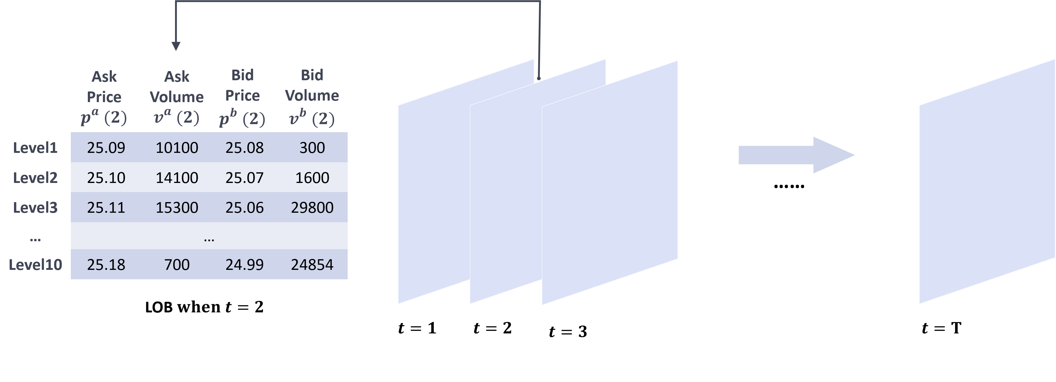
Unfortunately, it is not straightforward to apply LOB into existing discrepancy measures. Representative discrepancies like Euclidean distances [15, 16] and probabilistic distances [11] all require and to be vectorized inputs, while the time steps LOB is publicized in the form of normally a matrix data. That is, at each time step , the best price levels on both sides of LOB as well as the associated total volume of the untraded orders are output as . More specifically, , where and are for the -th price level and the associated total volume, and indicates the ask side and bid side (see Figure 1), respectively. Existing FMS works that calibrate mid-price can be viewed as simplifying LOB by averaging the best ask price and the best bid price at -th step, i.e., , which naturally lose much important information of the underlying data generative process.
This paper aims to learn a low-dimensional vectorized representation of the LOB data with the autoencoder, so that the well-established discrepancy measures can still be easily adopted for calibration. Ideally, if the output of the decoder closely resembles the input of the encoder, the latent vector is believed to be an effective representation of the input LOB. The key challenge lies in that the LOB involves not only the non-linear auto-correlation in the temporal axis but also the precedence between successive price levels at each time step. The literature witnesses increasing efforts on analyzing LOB data with neural networks, which, however, neither adopt the autoencoder framework nor explicitly study the vectorized representations. To accurately represent these two properties in the latent vector, the proposed encoder as well as the symmetric decoder contains three blocks, i.e., a fully connected network for extracting features of the price precedence, a Transformer stack for capturing the temporal auto-correlation, and another fully connected network for dimension reduction.
Three groups of experiments have been conducted. The empirical findings are as follows:
Finding 1: Calibrating LOB leads to better FMS than traditional mid-price calibration;
Finding 2: The vectorized representations of various LOB can be effectively learned, while the convolution layers adopted in existing works is not effective;
Finding 3: Better representation of LOB, better calibration of FMS.
The rest of this paper is organized as follows. Section 2 introduces the related works of FMS calibration and deep learning for LOB. Section 3 describes the proposed Transformer-based autoencoder in details. Section 4 reports 3 key empirical findings. The conclusion is drawn in Section 5.
2 Related Work
Calibration of FMS. Traditional FMS works focus on designing rule-based agents to imitate various trading behaviors. Though several phenomena generally existed in different stocks have been reproduced and explained by FMSs [17, 18], they received increasing criticisms for not being able to simulate any specific time series data but only macro properties of the market [19]. Since 2015, several calibration objectives have been proposed for FMS [10]. A straightforward way [15] is to simply calculate the mean square error (MSE) between the simulated mid-price vector and the observed mid-price vector. Methods of Simulated Moments calculate the statistical moments of both the observed and simulated mid-price, and measure the distances between the two vectors of moments as the discrepancy [16]. To better utilize the temporal properties of the mid-price vector, some information-theoretic criteria based discrepancies are proposed based on various time windows [20]. Francesco [21] tries to compares the distribution distance between the simulated and observed mid-price data. The Kolmogorov-Smirnov (K-S) test is generalized to multi-variate data, while their empirical verification was only conducted on the mid-price vector and the traded volume vector [11]. To summarize, existing calibration functions all require the vectorized input format and related works mainly calibrate to the mid-price data.
Deep Learning for LOB. Most of the studied tasks are to predict the price movement [22], a binary classification problem. Since classification with neural networks is known to be effective, the end-to-end solutions are naturally considered for predicting the price movement from LOB and the vectorized representation learning is not explicitly defined. In the contrary, since the FMS models are mostly rule-based (especially the matchmaking rule of updating the LOB), they are non-differentiable and cannot be trained end-to-end with the feature extraction layers. Thus, the vectorized representation learning need especial treatments in FMS.
Recent works propose to generate LOB data with deep learning, which is quite similar to the goal of FMS [23]. However, they do not involve any validation or calibration steps to force the generated data resembling any given observed LOB, but only limited to follow some macro properties of the market [24, 25]. Some of them also are not informed by the real-world matchmaking rules for updating LOB [26, 27]. These issues impose significant restrictions on the use of these models as simulators, since one can hardly intervene the order streams to do "what-if" test and reveal the micro-structured causes of certain financial events [5, 28]. Furthermore, they explicitly require the ground truth order streams as input to train the networks, which is not available in the setting of FMS calibration problems.
Among them, the convolution layers and Long-Short Term Memory (LSTM) are the mostly used architecture. Recently, the Transformer model is adopted instead of LSTM, but the convolution layers are still kept [29, 30]. This work argues for abandoning the convolution layer as it is empirically found ineffective to learning from LOB.
3 Method
To feed the LOB data to the well-established calibration functions who only accept the vectorized input, we propose to learn a function that can represent the time series LOB data in a vectorized latent space. The requirement of is two-fold. First, naturally constitutes a dimension reduction process. Suppose receives a step LOB , it is expected that with and . Second, within the latent space of , the information of LOB can be largely preserved for downstream calibration tasks. One verification is the existence of an inverse function such that resembles the original . To this end, the autoencoder architecture is considered, where constitutes the encoder network and is modeled by the decoder. The latent vector between the encoder and the decoder is the learned representation of , i.e., , and is the reconstructed data.
The Properties of LOB. The difficulty of the representation learning lies in the specific properties of LOB. First, the time series LOB is essentially auto-correlated between successive time steps, since is generated by updating with incoming order streams between the time interval . Second, comprises 10 levels of price and volume on both ask and bid sides. The price levels should strictly follow the precedence that prices at lower levels are worse than those at higher levels. That is, the bid/ask price at the -th level should be certainly larger/smaller than the -th level, where and . Hence, the encoder network should be able to effectively handle both the non-linear temporal auto-correlation and the precedence of price levels. On this basis, the proposed encoder is comprised of three components, i.e., the feature extraction block as a fully connected network (FCN, denoted as ), a Transformer stack, and the dimension reduction block as another FCN (denoted as ). The architecture of the encoder is depicted in Figure 2.
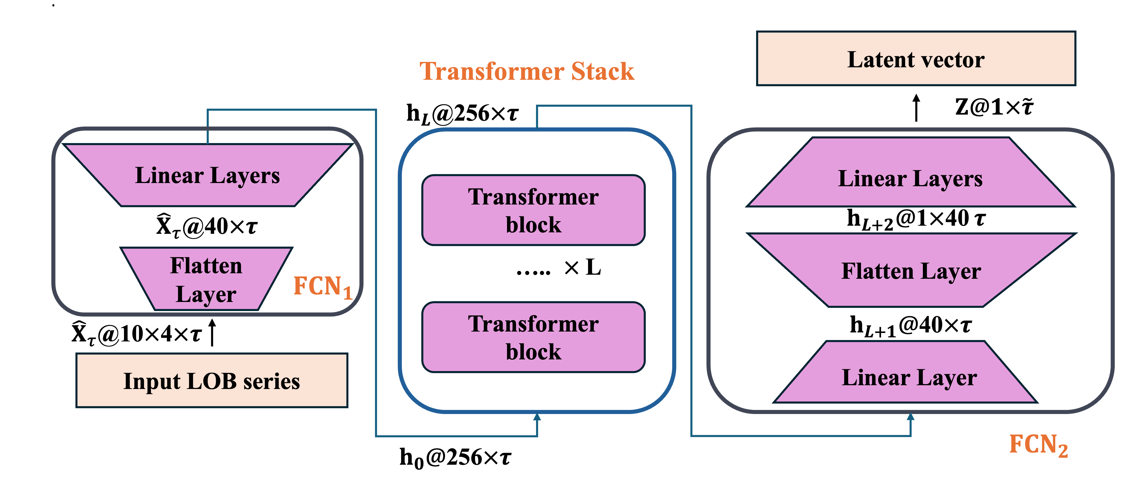
The Feature Extraction Block. The is designed for extracting useful features from LOB. Previous works that utilize machine learning methods for processing LOB data often pre-process a set of hand-crafted features to describe market dynamics [31]. Those works typically consider the price levels as independent features and seldom deal with the precedence relationship. Recent pioneer work [32] uses convolution neural networks (CNNs) to automatically extract the features from LOB. The intuition is that CNN may capture the precedence between the price levels through convolutions like what has been done to the pixels. However, the 10 levels of bid prices, bid volumes, ask prices, and ask volumes, have quite different scales and meanings, which is non-trivial to be convolved adequately. This work utilizes the FCN for feature extraction by . First, the LOB at each time step is flattened from to using 1 linear layer. That is, the flattened is into . The times series LOB is accordingly flattened in and then projected into higher-dimensional space of to obtain a more diverse range of features, using also 1 linear layer.
The Transformer Block. The second component of the encoder is the Transformer stack with linked vanilla Transformers [33]. It aims to learn the temporal auto-correlation between successive time steps with the multi-headed self-attention (MSA), feed-forward layer (or say FCN), and layernorm (LN). Specifically, at each -th stacked Transformer, it computes
| (1) | |||||
| (2) |
where is the output of the whole Transformer stack as well as the input of .
The Dimension Reduction Block. Note that, the Transformer does not change the data space and thus . The is designed to reduce the dimensionality of so that the LOB can be represented as the latent vector . For that purpose, we need to first flatten as a vector using 1 linear layer. Notice that, direct concatenating each of 256 rows of as a vector will lead to too large input for the successive layers of dimension reduction. Hence, we first project to with 1 linear layer. Then the is flattened by concatenating its 40 rows to produce a vector using 1 linear layer. At last, 3 linear layers are carried out to reduce to .
The Decoder. The architecture of the decoder keeps symmetric to the encoder. The latent vector first passes a network upside-down of to increase its dimension back to . Subsequently, the output of undergoes a stack of vanilla Transformers. Finally, the output of the Transformers stack goes through another FCN that is upside-down of to obtain the reconstructed data .
Implementation Details. The proposed autocoder is named as SimLOB. To keep the size of SimLOB computationally tractable, the observed steps LOB is first split into multiple segments, each of which contains time steps as suggested by [22]. Through sensitive analysis in Appendix E, we set and by default. Given a pair of an original and its reconstructed with the length of steps, the reconstruction error calculates . And defines the training loss given pairs of training data sequences, by averaging the reconstruction errors on the training data with batch size . SimLOB is trained by Adam [34] with learning rate 1E-4 for 200 epochs.
4 Empirical Studies
The following three research questions (RQs) are majorly concerned in this work.
RQ-1: Can we learn to represent various LOB into vectors? What is the recommended architecture?
RQ-2: Does "better representation of LOB, better calibration of FMS" generally hold?
RQ-3: Is it really beneficial to calibrate FMS with LOB instead of traditional mid-price?
Three groups of experiments are conducted accordingly. Group-1: the proposed SimLOB is trained with large volume of synthetic LOB data, together with 8 state-of-the-art (SOTA) networks. The reconstruction errors on both synthetic and real testing data are measured to assess the quality of the vectorized representations. The parameter sensitivity of SimLOB is also analyzed in terms of both reconstruction and calibration. Group-2: for the above 9 networks, the represented latent vectors are applied to 10 FMS calibration tasks to show the consistency between the reconstruction errors and the calibration errors. Group-3: the calibration errors in terms of the vector representation learned by SimLOB, the raw LOB and the extracted mid-price are compared.
4.1 General Experimental Setup
The FMS Model. The widely studied Preis-Golke-Paul-Schneid (PGPS) model is adopted as the FMS model [35], which models all the traders as two types of agents: 1) 125 liquidity providers who submit limited orders; 2) 125 liquidity takers who submit market orders and cancel untraded limited orders in the LOB. The detailed workflow and configurations can be found in Appendix B.1. In short, the PGPS model contains 6 parameters to be calibrated.
The Dataset for Representation Learning. In the literature, augmenting the training data with the synthetic LOB data generated by FMS is increasingly popular [23, 27]. Hence, this work trains the SimLOB with purely the synthetic LOB data generated by the PGPS model with different parameters. In general, each setting of the 6-parameter tuple of PGPS actually defines a specific market scenario. To ensure the synthetic data enjoys enough diversity, we uniformly randomly sample 2000 different settings of those 6-parameter tuples from a predefined range suggested by [19] (see Appendix B.2). The PGPS runs with each setting to generate one simulated LOB for 50000 time steps, simulating 50000 seconds of the market. Then we split each of the 2000 LOB data as 500 sequences with 100 time steps. Thus, there are 1 million LOB sequences with , where 80% of those synthetic data is randomly sampled for training, and the rest 20% is taken as testing data. The real market data from the sz.000001 stock of Chinese market (during May of 2019) is also used to test the trained networks.
The Compared Networks. In the literature, several networks have been designed for analyzing LOB data [22]. Although their tasks main focus on a different task of price trend prediction, they are indeed attempts of dealing with time series LOB. This experiment selects 7 SOTA networks by taking their architecture before the last linear layer as their representation learning layers, and all share . We follow the conventions of [22] to name the 8 networks as MLP[36], LSTM[36], CNN1[37], CNN2[38], CNN-LSTM[38], DeepLOB[32], TransLOB[30]. As their names suggested, despite that MLP, LSTM, CNN1, and CNN2 adopt single type networks, the other works mostly employ a Convolution-Recurrent based architecture to intuitively first extract the prices precedence and then capture the temporal auto-correlation. TransLOB employs the Transformer architecture to replace the recurrent network while still keeping the convolution layers. Their input formats and sizes follow the suggestions of their original papers and are shown in Appendix C. TransLOB-L is an enlarged version of TransLOB to keep the size approximately aligned with SimLOB, by using 7 stacked Transformers instead of 2 as in original TransLOB. All the 8 compared networks are trained in the same protocol with SimLOB.
The Calibration Tasks. The 10 synthetic LOB data are generated with 10 different settings of 6-parameter tuples (see Appendix B.2), each of which contains time steps, i.e., simulating 1 hour of the market at the frequency of 1 second. These 10 synthetic data are utilized as the target data for calibrating PGPS. Note that these data instances are challenging that they have a much higher frequency than traditional FMS works who can only calibrate to daily data [19]. And the length of the target data is also at least longer than the existing calibration works [10]. The objective function for calibration employs MSE. For calibrating the mid-prices as traditional works do, Eq.(3) gives
| (3) |
where . For calibrating the learned latent vectors as this paper proposes, the calibration function is slightly different. Both the target and simulated LOB with time steps is represented as latent vectors, each of which has the length of . Then we have Eq.(4)
| (4) |
4.2 Group-1: Learning the Vectorized Representations of LOB
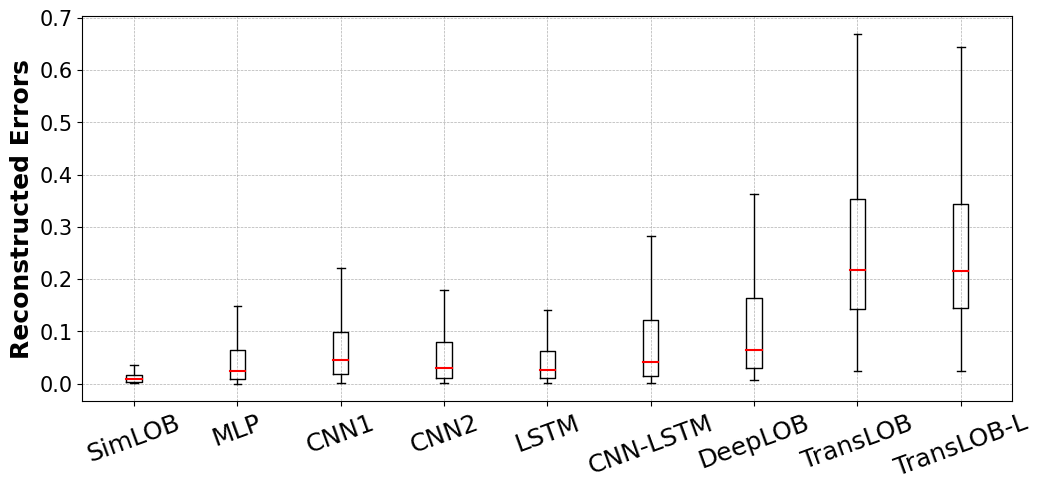
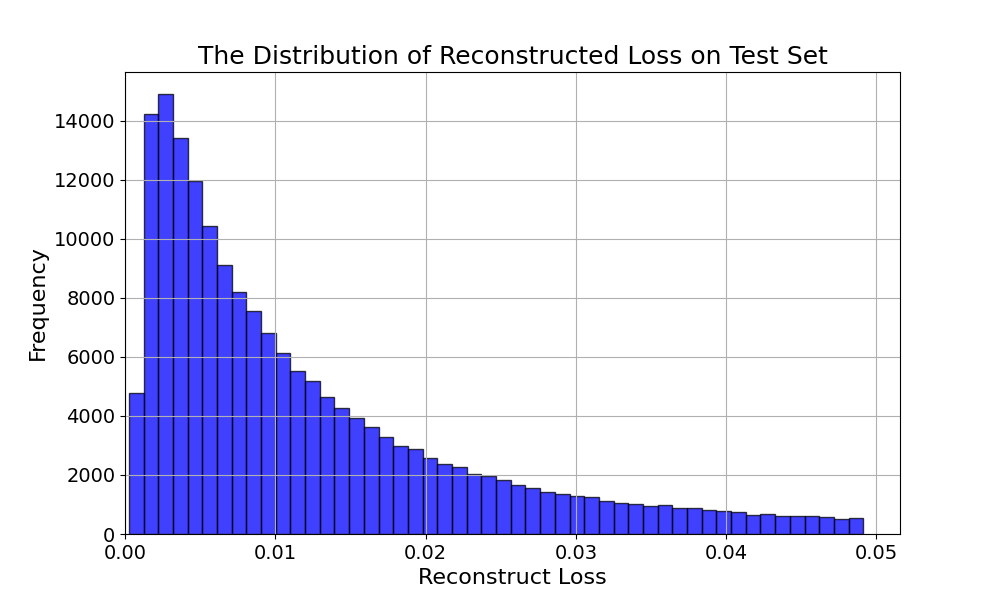
The reconstruction errors on 0.2 million synthetic testing data of all 9 compared algorithms are depicted in Figure 3(a). Among them, SimLOB not only achieves the smallest averaged reconstruction error, but performs the stablest. Specifically, the distribution of the reconstruction errors of SimLOB follows a power law distribution with a mode of 0.003 (See Figure 7 of Appendix D). Almost all the CNN-based networks perform the worst, suggesting that CNN is not effective as expected to deal with LOB data. This is quite contradictory to the trend of existing works on deep learning for LOB.
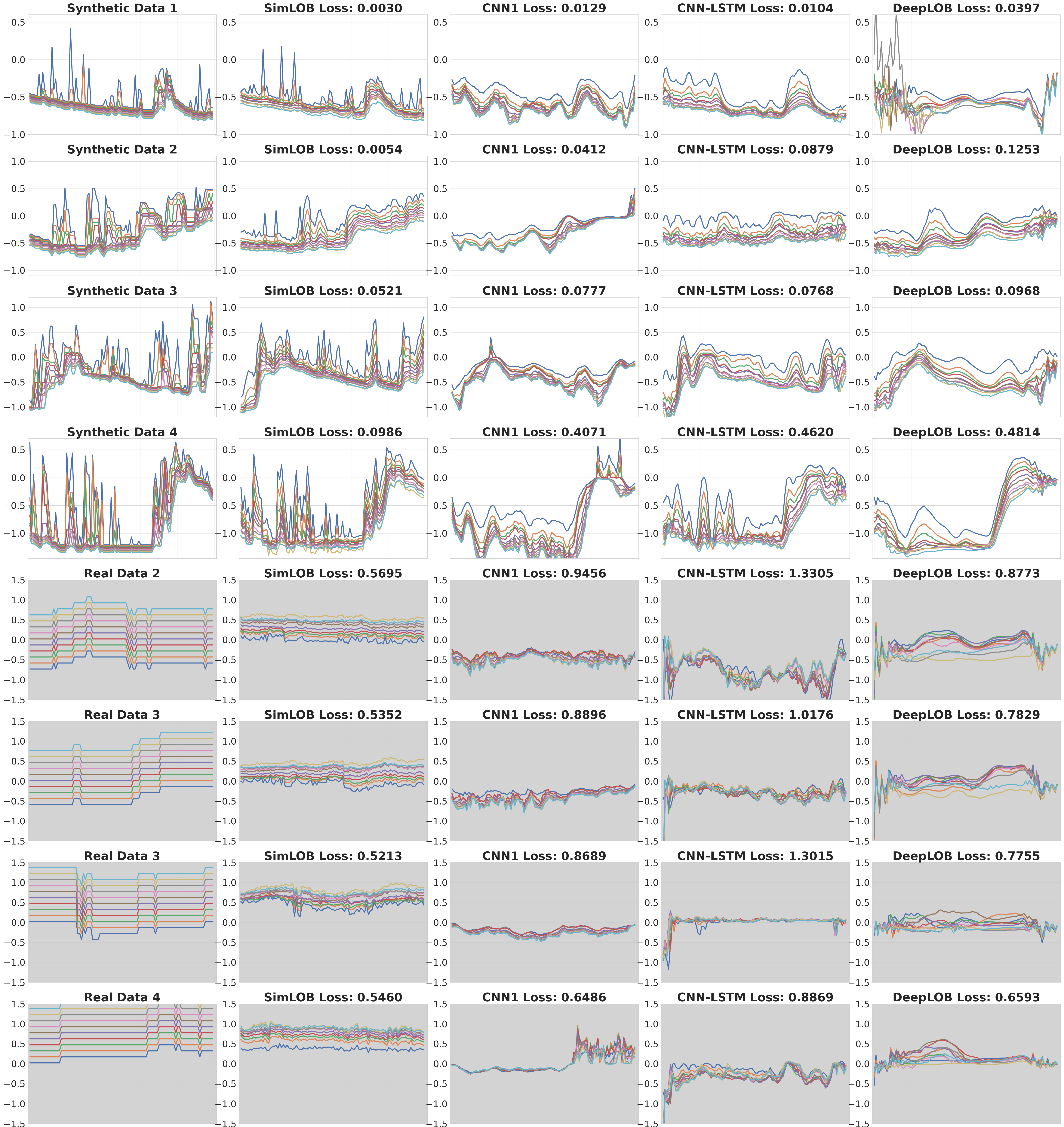
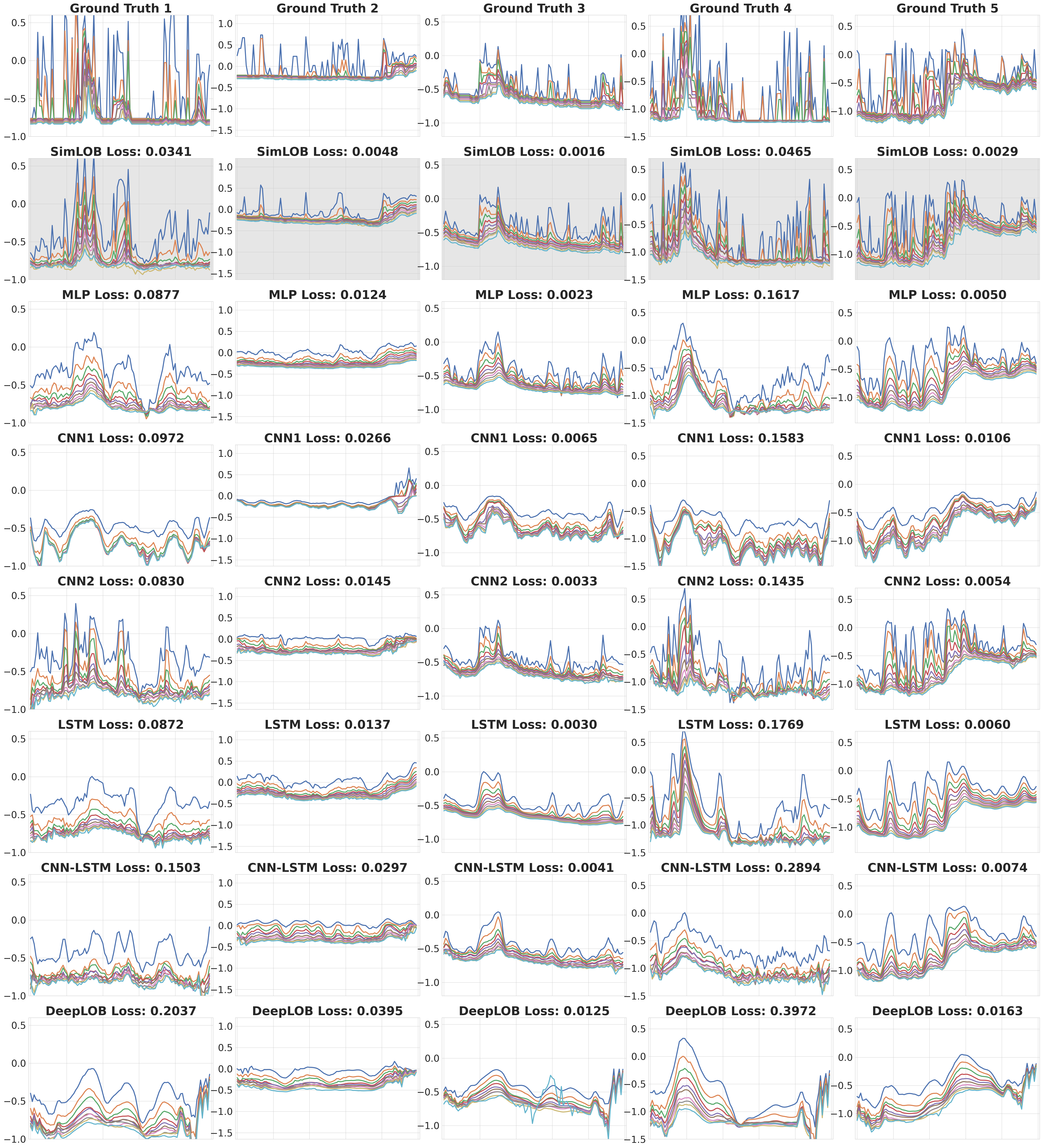
Next, as shown in the first 4 rows of Figure 4, the 10 levels of bid prices of 4 randomly selected synthetic data and the reconstructed LOB of 4 networks are visualized. For the visualizations on more data and networks, please refer to Figure 8 of Appendix D. It is clear that the reconstructed data of SimLOB successfully captures many details of the target LOB, especially the fluctuations and the precedence of the 10 price levels. Comparatively, the other networks perform quite poorer as their reconstructed price levels are smoothed. This implies that they do not preserve the information between both time steps and price levels.
Note that, these network are trained purely on synthetic data. We directly apply them to reconstruct real market data. As seen in the last 4 rows of Figure 4, the real LOB fluctuates quite slightly comparing to synthetic data. SimLOB can still capture the information of price precedence well and the fluctuations to some extent, though the range of prices deviates. Contrarily, the compared networks all fail to reconstruct meaningful details. This suggests that SimLOB can be further generalized to more diverse LOB with special treatments, such as training with real data. The structural settings of SimLOB are analyzed in Appendix E, which suggests and .
4.3 Group-2: Better Representation, Better Calibration
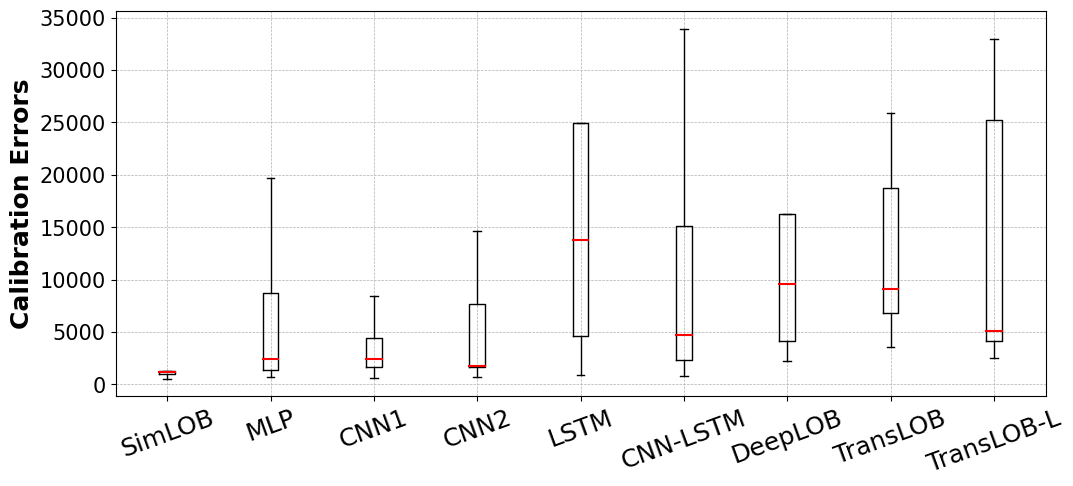
Each of the 10 synthetic LOB data with is first applied to 9 compared networks to obtain the latent vectors, respectively. Then we apply Eq.(4) and PSO to PGPS to obtain the best-found parameter tuple and the corresponding simulated data. For each network, the calibration error between the target data and the simulated data is calculated using . The detailed calibration errors are listed in Table 1. The best result between TransLOB and TransLOB-L is listed here. Among all the learned representations, the ones learned by SimLOB lead to the best calibration performance on 7 out of 10 instances and the runner-up performance on data 1 and data 9. The distribution of the calibration errors (outliers omitted) in Figure 3(b) show the advantages of SimLOB more clearly. Furthermore, by comparing Figure 3(a) and Figure 3(b), it can be observed that the reconstruction errors and the calibration errors are consistent, which implies that the better the representation of LOB is, the better the calibration of FMS is highly likely to be.
| SimLOB | MLP | CNN1 | CNN2 | LSTM | CNNLSTM | DeepLOB | TransLOB | |
|---|---|---|---|---|---|---|---|---|
| data1 | 1.27E03 | 2.41E03 | 1.69E03 | 1.65E03 | 8.98E02 | 2.32E03 | 9.60E03 | 3.53E03 |
| data2 | 1.30E03 | 1.85E03 | 1.61E03 | 5.67E03 | 2.43E04 | 1.51E04 | 4.14E03 | 2.52E04 |
| data3 | 4.35E02 | 6.95E02 | 6.05E02 | 6.57E03 | 1.13E03 | 1.47E03 | 2.18E03 | 2.55E03 |
| data4 | 5.51E02 | 1.10E03 | 2.79E03 | 1.53E03 | 4.57E03 | 8.27E02 | 2.27E03 | 1.15E04 |
| data5 | 1.20E03 | 8.70E03 | 1.19E04 | 1.74E03 | 2.49E04 | 4.72E03 | 1.63E04 | 4.77E03 |
| data6 | 8.58E03 | 2.11E04 | 2.87E04 | 1.34E04 | 1.07E05 | 3.40E04 | 8.42E04 | 3.29E04 |
| data7 | 1.49E06 | 3.07E05 | 1.11E06 | 1.09E06 | 3.74E06 | 1.62E06 | 1.92E06 | 1.60E06 |
| data8 | 1.07E03 | 2.38E03 | 3.03E03 | 1.84E03 | 1.37E04 | 2.61E03 | 8.80E03 | 5.08E03 |
| data9 | 1.13E04 | 1.97E04 | 8.42E03 | 1.46E04 | 6.68E04 | 2.21E04 | 6.41E04 | 2.68E04 |
| data10 | 9.83E02 | 1.36E03 | 1.98E03 | 4.30E04 | 1.31E04 | 8.28E03 | 1.51E04 | 4.12E03 |
4.4 Group-3: Calibrating Vectorized LOB is Beneficial
To demonstrate that calibrating LOB is beneficial to FMS, the above 10 synthetic LOB data is also calibrated using traditional objective function Eq.(3) with merely mid-prices, denoted as Cali-midprice. Furthermore, one may concern why not directly use the reconstruction error as the calibration function to calibrate the raw LOB. Hence, we also calibrate PGPS to the raw LOB, denoted as Cali-rawLOB.
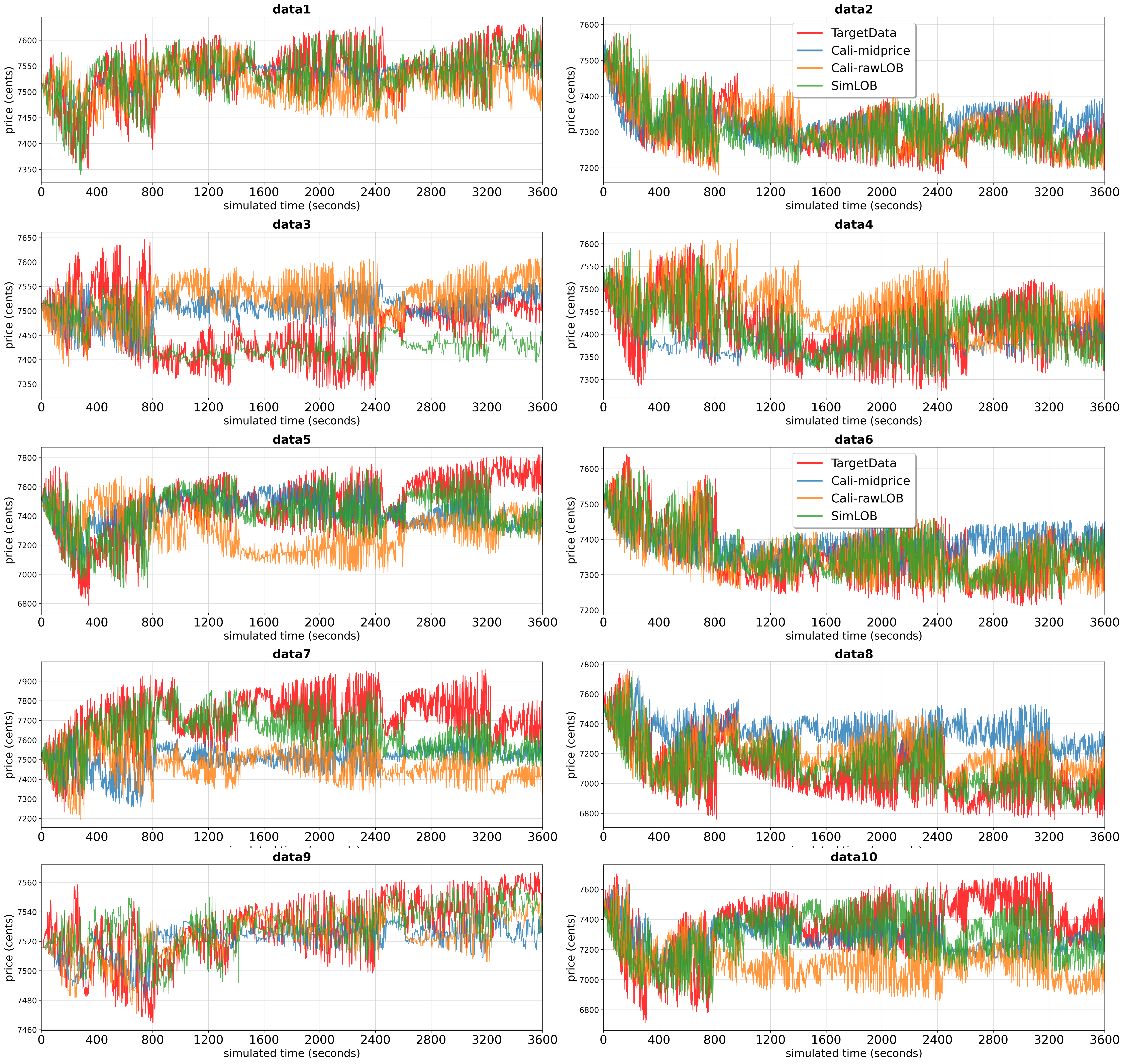
Table 7 in Appendix F shows that SimLOB almost dominates Cali-midprice and Cali-rawLOB. The simulated mid-prices of SimLOB, Cali-rawLOB, and Cali-midprice on 10 target data are also depicted in Figure 5. It can be intuitively seen that the simulated mid-price of SimLOB resembles the target data much more than Cali-rawLOB and Cali-midprice. Comparing SimLOB with Cali-rawLOB, essentially measures the MSE value between two very long vectors with the length of on each segmentation. Though it can tell the difference between two raw LOB data, it does not reflect the importance of the key properties of temporal auto-correlation and the price precedence. Comparing to Cali-midprice, SimLOB helps PGPS achieve much better performance on not only the whole LOB but also the mid-price, simply because the mid-price is basically a derivate of LOB. To summarize, calibrating with more information of the market can help improve the fidelity of the simulation, but needs effective latent representations. This supports the initial motivation of this work.
5 Conclusions
This paper proposes to learn the vectorized representations of the LOB data, the fundamental data in financial market. The autoencoder framework is employed for this purpose, and the latent vector is taken as the representation. In the literature, there have been increasing research works focusing on analyzing LOB data with neural networks. However, they did not use the autoencoder framework, neither explicitly learned the vectorized representations. This work studies 8 SOTA neural architectures for LOB, and discusses that the commonly used convolution layers are not effective for preserving the specific properties of LOB. Based on that, a novel neural architecture is proposed with three components: the first fully connected network for extracting the features of price precedence from LOB, the stacked Transformers for capturing the temporal auto-correlation, and the second fully connected network for reducing the dimensionality of the latent vector. Empirical studies verify the advantages of the proposed network in terms of the reconstruction errors against existing neural networks for LOB. Moreover, it is found that the effectiveness of the representation learning positively correlated with the downstream tasks of calibrating financial market simulation model. Further empirical findings support that the financial market simulation models should be calibrated with compactly represented LOB data rather than merely mid-prices or raw LOB data.
References
- [1] A. J. Menkveld and B. Z. Yueshen, “The flash crash: A cautionary tale about highly fragmented markets,” Management Science, vol. 65, no. 10, pp. 4470–4488, 2019.
- [2] J. Paulin, A. Calinescu, and M. Wooldridge, “Understanding flash crash contagion and systemic risk: A micro–macro agent-based approach,” Journal of Economic Dynamics and Control, vol. 100, pp. 200–229, 2019.
- [3] X. Wang and M. P. Wellman, “Spoofing the limit order book: An agent-based model,” in Proceedings of the 16th International Conference on Autonomous Agents and Multiagent Systems (AAMAS 2017), (Brazil), pp. 651–659, May 2017.
- [4] J. D. Farmer and D. Foley, “The economy needs agent-based modelling,” Nature, vol. 460, no. 7256, pp. 685–686, 2009.
- [5] V. Darley, A NASDAQ market simulation: insights on a major market from the science of complex adaptive systems, vol. 1. World Scientific, 2007.
- [6] A. Madhavan, “Market microstructure: A survey,” Journal of financial markets, vol. 3, no. 3, pp. 205–258, 2000.
- [7] J. M. Hofman, D. J. Watts, S. Athey, F. Garip, T. L. Griffiths, J. Kleinberg, H. Margetts, S. Mullainathan, M. J. Salganik, S. Vazire, et al., “Integrating explanation and prediction in computational social science,” Nature, vol. 595, no. 7866, pp. 181–188, 2021.
- [8] R. L. Axtell and J. D. Farmer, “Agent-based modeling in economics and finance: Past, present, and future,” Journal of Economic Literature, 2022.
- [9] A. Fabretti, “On the problem of calibrating an agent based model for financial markets,” Journal of Economic Interaction and Coordination, vol. 8, pp. 277–293, 2013.
- [10] D. Platt, “A comparison of economic agent-based model calibration methods,” Journal of Economic Dynamics and Control, vol. 113, p. 103859, 2020.
- [11] Y. Bai, H. Lam, T. Balch, and S. Vyetrenko, “Efficient calibration of multi-agent simulation models from output series with bayesian optimization,” in Proceedings of the Third ACM International Conference on AI in Finance, pp. 437–445, 2022.
- [12] J. Grazzini, M. G. Richiardi, and M. Tsionas, “Bayesian estimation of agent-based models,” Journal of Economic Dynamics and Control, vol. 77, pp. 26–47, 2017.
- [13] R. Kozhan and M. Salmon, “The information content of a limit order book: The case of an fx market,” Journal of Financial Markets, vol. 15, no. 1, pp. 1–28, 2012.
- [14] C. Chiarella and G. Iori, “A simulation analysis of the microstructure of double auction markets,” Quantitative finance, vol. 2, no. 5, p. 346, 2002.
- [15] M. C. Recchioni, G. Tedeschi, and M. Gallegati, “A calibration procedure for analyzing stock price dynamics in an agent-based framework,” Journal of Economic Dynamics and Control, vol. 60, pp. 1–25, 2015.
- [16] J. Grazzini and M. Richiardi, “Estimation of ergodic agent-based models by simulated minimum distance,” Journal of Economic Dynamics and Control, vol. 51, pp. 148–165, 2015.
- [17] I. Palit, S. Phelps, and W. L. Ng, “Can a zero-intelligence plus model explain the stylized facts of financial time series data?,” in Proceedings of the 11th International Conference on Autonomous Agents and Multiagent Systems-Volume 2, pp. 653–660, Citeseer, 2012.
- [18] S. Vyetrenko, D. Byrd, N. Petosa, M. Mahfouz, D. Dervovic, M. Veloso, and T. Balch, “Get real: Realism metrics for robust limit order book market simulations,” in Proceedings of the First ACM International Conference on AI in Finance, pp. 1–8, 2020.
- [19] D. Platt and T. Gebbie, “Can agent-based models probe market microstructure?,” Physica A: Statistical Mechanics and its Applications, vol. 503, pp. 1092–1106, 2018.
- [20] S. Barde, “A practical, accurate, information criterion for nth order markov processes,” Computational Economics, vol. 50, no. 2, pp. 281–324, 2017.
- [21] F. Lamperti, “An information theoretic criterion for empirical validation of simulation models,” Econometrics and Statistics, vol. 5, pp. 83–106, 2018.
- [22] M. Prata, G. Masi, L. Berti, V. Arrigoni, A. Coletta, I. Cannistraci, S. Vyetrenko, P. Velardi, and N. Bartolini, “Lob-based deep learning models for stock price trend prediction: a benchmark study,” Artificial Intelligence Review, vol. 57, no. 5, pp. 1–45, 2024.
- [23] S. A. Assefa, D. Dervovic, M. Mahfouz, R. E. Tillman, P. Reddy, and M. Veloso, “Generating synthetic data in finance: opportunities, challenges and pitfalls,” in Proceedings of the First ACM International Conference on AI in Finance, pp. 1–8, 2020.
- [24] A. Coletta, M. Prata, M. Conti, E. Mercanti, N. Bartolini, A. Moulin, S. Vyetrenko, and T. Balch, “Towards realistic market simulations: a generative adversarial networks approach,” in Proceedings of the Second ACM International Conference on AI in Finance, pp. 1–9, 2021.
- [25] A. Coletta, A. Moulin, S. Vyetrenko, and T. Balch, “Learning to simulate realistic limit order book markets from data as a world agent,” in Proceedings of the Third ACM International Conference on AI in Finance, pp. 428–436, 2022.
- [26] J. Li, X. Wang, Y. Lin, A. Sinha, and M. Wellman, “Generating realistic stock market order streams,” in Proceedings of the AAAI Conference on Artificial Intelligence, vol. 34, pp. 727–734, 2020.
- [27] D. Cao, Y. El-Laham, L. Trinh, S. Vyetrenko, and Y. Liu, “A synthetic limit order book dataset for benchmarking forecasting algorithms under distributional shift,” in NeurIPS 2022 Workshop on Distribution Shifts: Connecting Methods and Applications, 2022.
- [28] L. Hamill and N. Gilbert, Agent-based modelling in economics. John Wiley & Sons, 2015.
- [29] P. Yang, L. Fu, J. Zhang, and G. Li, “Ocet: One-dimensional convolution embedding transformer for stock trend prediction,” in International Conference on Bio-Inspired Computing: Theories and Applications, pp. 370–384, Springer, 2022.
- [30] J. Wallbridge, “Transformers for limit order books,” arXiv preprint arXiv:2003.00130, 2020.
- [31] A. Ntakaris, M. Magris, J. Kanniainen, M. Gabbouj, and A. Iosifidis, “Benchmark dataset for mid-price forecasting of limit order book data with machine learning methods,” Journal of Forecasting, vol. 37, no. 8, pp. 852–866, 2018.
- [32] Z. Zhang, S. Zohren, and S. Roberts, “Deeplob: Deep convolutional neural networks for limit order books,” IEEE Transactions on Signal Processing, vol. 67, no. 11, pp. 3001–3012, 2019.
- [33] A. Vaswani, N. Shazeer, N. Parmar, J. Uszkoreit, L. Jones, A. N. Gomez, Ł. Kaiser, and I. Polosukhin, “Attention is all you need,” Advances in neural information processing systems, vol. 30, 2017.
- [34] D. P. Kingma and J. Ba, “Adam: A method for stochastic optimization,” arXiv preprint arXiv:1412.6980, 2014.
- [35] T. Preis, S. Golke, W. Paul, and J. J. Schneider, “Multi-agent-based order book model of financial markets,” Europhysics Letters, vol. 75, no. 3, p. 510, 2006.
- [36] A. Tsantekidis, N. Passalis, A. Tefas, J. Kanniainen, M. Gabbouj, and A. Iosifidis, “Using deep learning to detect price change indications in financial markets,” in 2017 25th European signal processing conference (EUSIPCO), pp. 2511–2515, IEEE, 2017.
- [37] A. Tsantekidis, N. Passalis, A. Tefas, J. Kanniainen, M. Gabbouj, and A. Iosifidis, “Forecasting stock prices from the limit order book using convolutional neural networks,” in 2017 IEEE 19th conference on business informatics (CBI), vol. 1, pp. 7–12, IEEE, 2017.
- [38] A. Tsantekidis, N. Passalis, A. Tefas, J. Kanniainen, M. Gabbouj, and A. Iosifidis, “Using deep learning for price prediction by exploiting stationary limit order book features,” Applied Soft Computing, vol. 93, p. 106401, 2020.
- [39] Y. Shi and R. Eberhart, “A modified particle swarm optimizer,” in Proceedings of 1998 IEEE international conference on evolutionary computation, pp. 69–73, IEEE, 1998.
- [40] P. Belcak, J.-P. Calliess, and S. Zohren, “Fast agent-based simulation framework with applications to reinforcement learning and the study of trading latency effects,” in International Workshop on Multi-Agent Systems and Agent-Based Simulation, pp. 42–56, Springer, 2021.
Appendix A Computational Resources
The experiments run on a server with 250GB memory, the Intel(R) Xeon(R) Gold 5218R CPU @ 2.10GHz with 20 physical cores, and 2 NVIDIA RTX A6000 GPU. The training of each network on average requires around 50 hours in the data parallel manner with 2 A6000 GPU. The calibration of each LOB data sequence costs 2-3 hours with 20 CPU cores or say 40 threads. The simulator can only run on a single core, while the PSO can be run in parallel with 40 simulators.
Appendix B The PGPS Financial Market Simulation Model
B.1 The Details of PGPS
The Preis-Golke-Paul-Schneid (PGPS) model is a representative FMS model [35], which models all the traders in the market as two types of agents: 125 liquidity providers and 125 liquidity takers. The entire simulation flowchart can be seen in Figure 6.
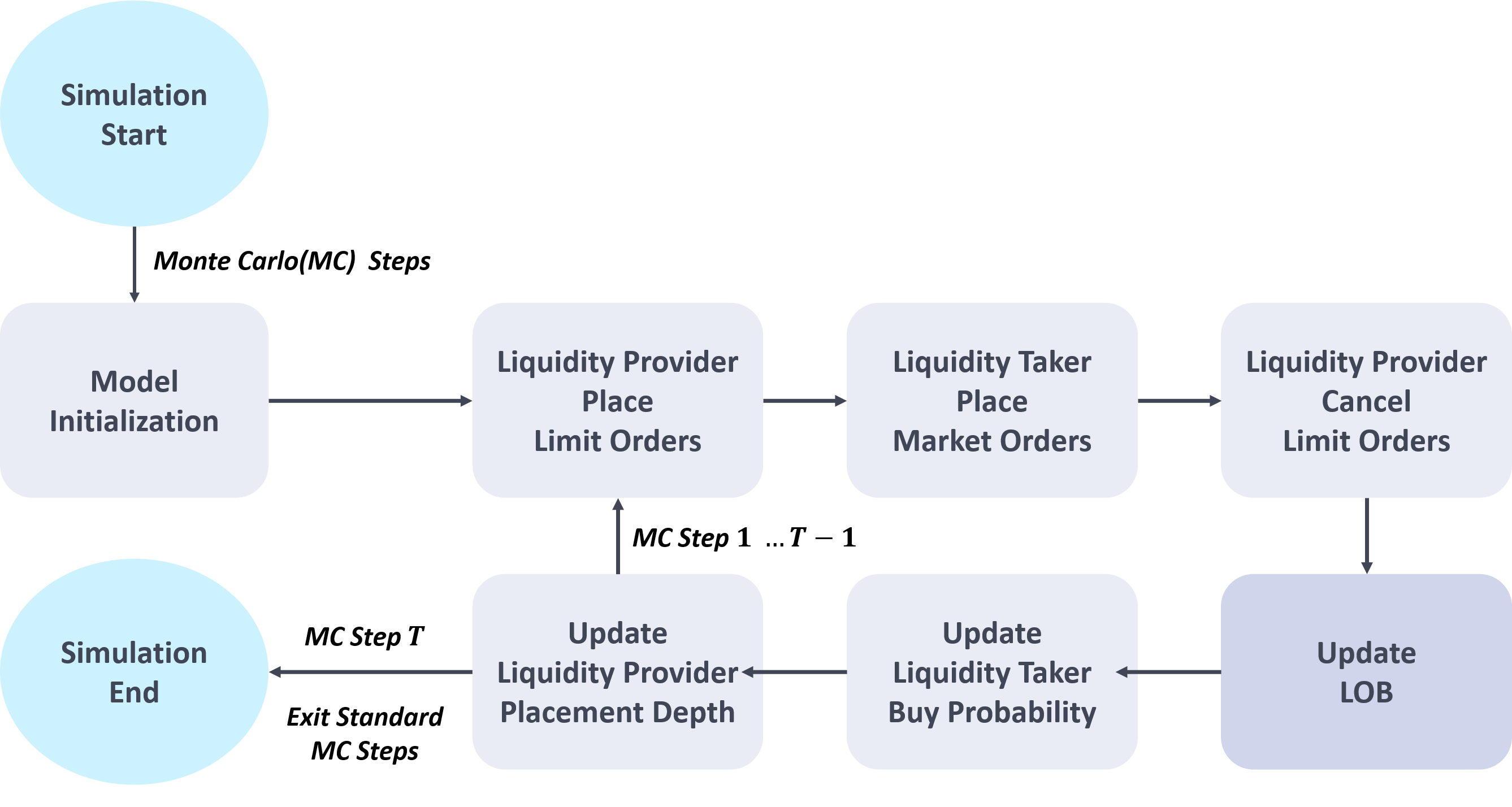
The detailed settings are as follows. At each -th time step, each liquidity provider may submit a limited order with a fixed probability of . The probability of each limited order being either the bid side or ask side is set to 0.5. Each liquidity taker may submit a market order at a fixed probability and cancel an untraded limited order with a probability . The probability of the market order being either the bid side or ask side is and , respectively. The is determined by a mean-reverting random walk with a mean of 0.5, and the mean reversion probability equals to . The increment size towards the mean is controlled by . Each liquidity taker may also cancel an untraded limited order with a probability . For each order, the volume is fixed to 100 shares. The price of an ask limited order is determined by and the price of a bid limited order is calculated as , where . Here indicates a pre-computed value obtained by taking the average of Monte Carlo iterations of before simulation. is a uniform random number. The price of the market order is automatically set to the best price level at the opposite side. In summary, the PGPS model contains 250 agents and the key parameters to be calibrated are .
B.2 Generating Synthetic LOB by Randomly Sampling 6 PGPS Parameters
| Para. | Range | Remarks |
|---|---|---|
| Controlling the price of each limited order. | ||
| Controlling the price of each limited order. | ||
| Controlling the probability of the side of a market order (ask or bid). | ||
| The probability for each liquidity provider to submit a limited order. | ||
| The probability for each liquidity taker to submit a market order. | ||
| The probability for each liquidity taker to cancel an untraded order. |
The 10 calibration tasks with respect to synthetic data are also generated by randomly sampling from these ranges and simulating with . Here, we list the 10 groups of parameters in Table 3 for clarity.
| Parameters | ||||||
|---|---|---|---|---|---|---|
| data 1 | 80 | 8 | 0.1 | 0.02 | 0.002 | 0.02 |
| data 2 | 120 | 11 | 0.2 | 0.03 | 0.003 | 0.03 |
| data 3 | 130 | 12 | 0.3 | 0.04 | 0.003 | 0.04 |
| data 4 | 90 | 9 | 0.15 | 0.02 | 0.001 | 0.02 |
| data 5 | 70 | 7 | 0.15 | 0.015 | 0.0015 | 0.03 |
| data 6 | 134.64 | 15.45 | 0.3275 | 0.07116 | 0.002 | 0.0324 |
| data 7 | 17.7 | 11.36 | 0.2639 | 0.067 | 0.00066 | 0.03644 |
| data 8 | 153.53 | 9.27 | 0.2983 | 0.07343 | 0.00238 | 0.01278 |
| data 9 | 48.13 | 3.54 | 0.4374 | 0.02645 | 0.00077 | 0.01674 |
| data 10 | 7.13 | 7.04 | 0.1106 | 0.05609 | 0.00217 | 0.01389 |
Appendix C The Characteristics of the Compared Networks
The characteristics of the 9 compared networks are listed as in Table 4. The second and third columns give the acceptable input formats of each network, and the last column shows the sizes of the networks. The MLP has the largest size of 2.2E7 weights, which can be simply considered as the enlarged version of solely the proposed . In this regard, by comparing SimLOB with MLP, we know that the Transformer stacks are important to SimLOB. By comparing SimLOB and TransLOB-L, we know that more Transformer does not lead to better results (verified later in Figure 9 of Appendix E), the CNN should be abandoned and the linear layers of and are helpful.
| The length of time series | The size of | trainable parameters | |
|---|---|---|---|
| MLP | 100 | 40 | 2.2E7 |
| LSTM | 100 | 40 | 1.6E4 |
| CNN1 | 100 | 40 | 3.5E4 |
| CNN2 | 300 | 40 | 2.8E5 |
| CNN-LSTM | 300 | 42 | 5.3E4 |
| DeepLOB | 100 | 40 | 1.4E5 |
| TransLOB | 100 | 40 | 1.1E5 |
| TransLOB-L | 100 | 40 | 1.5E7 |
| SimLOB | 100 | 40 | 1.3E7 |
C.1 The Calibration Algorithm
Note that is basically a software simulator. In this work, it is programmed on the Multi-Agent Exchange Environment (MAXE)111https://github.com/maxe-team/maxe environment developed by University of Oxford with the MIT Lisence [40]. Thus the calibration problem does not enjoy useful mathematical properties like gradients. It is reasonable that more advanced black-box optimization algorithms can lead to better calibration errors. Here, for simplicity, a standard Particle Swarm Optimizer (PSO) is employed for optimizing the above problem [39]. The hyper-parameters of PSO follow the suggested configurations, where the population size is set to 40, the inertia weight is set to 0.8, the cognitive and social crossover parameters . The total iteration number of PSO in each run is fixed to 100 [10].
Appendix D More Results of the Reconstruction Errors
The trained SimLOB is tested on 0.2 million LOB sequences with 100 time steps. The distribution of the reconstruction error on each testing data is depicted in Figure 7, which follows a power law distribution with a mode of 0.003, implying that SimLOB performs quite stable on different LOB data.
In addition to Figure 4 in the main context, we depict the reconstructed data of the compared networks on 5 more synthetic data to demonstrate the superiority of SimLOB. In Figure 8, the reconstructed data of all the compared networks except for TransLOB and TransLOB-L are visualized. The situation remains the same that the reconstructed data of SimLOB resembles the target data to the most. The other networks have smoothed the target data to some extent, indicating that they are unable to fully preserve the key properties of LOB in their latent vectors. The reason of not depicting TransLOB and TransLOB-L is simply that their reconstructed data look like almost flat.
Appendix E Sensitive Analysis on the Structural Parameters of SimLOB
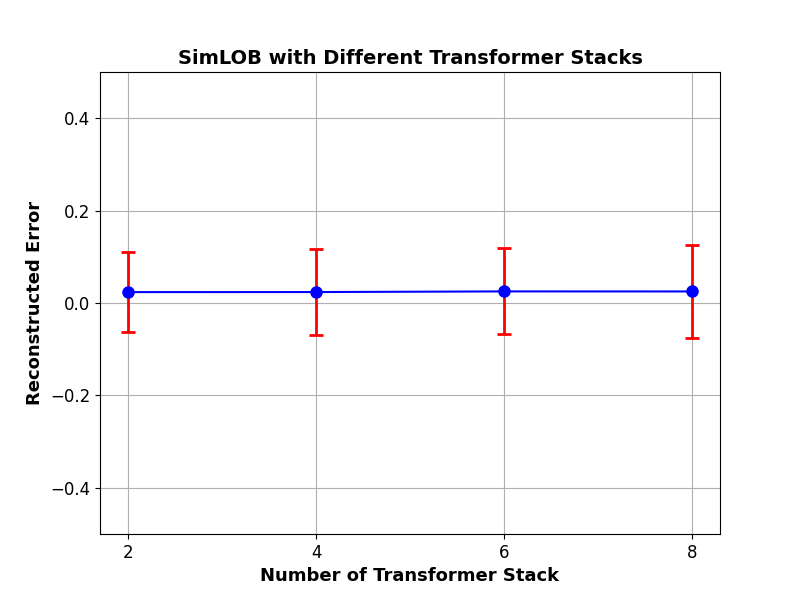
To analyze the architecture settings in SimLOB, we made the following counterparts of SimLOB. The number of stacks in Transformer block is adjusted as 2, 4, 6 and 8, respectively. The length of the latent vector is set to 64, 128, 256, and 512, respectively. The resultant variants of SimLOB are denoted as , , , and , where SimLOB with is found the best choice for default settings.
E.1 On the number of Transformer Stack
In the main context, the number of Transformer stack is recommended as . Actually, with , we found that the choice of did not influence the reconstruction errors much, as shown in Figure 9. That is, the reconstructed errors on 0.2 million testing data are around 0.025 for the 4 variants of SimLOB, and the standard deviation remains similarly, i.e., about 0.095. As adding one Transformer stack leads to around 1.5 millions more weights, we thus use the smallest tested value of as the default setting for SimLOB.
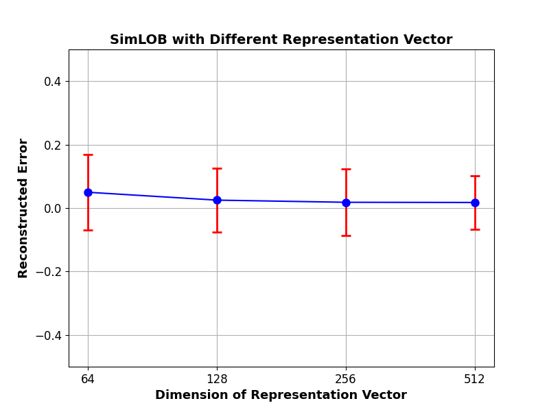
E.2 On the Length of Representation Vector
The default setting of the length of the learned representation vector is . Such setting is based on the sensitive analysis on the parameter with different choices like 64, 128, 256, and 512. That is, we train SimLOB with those settings separately and tested on the 0.2 million testing data. The reconstructed errors are listed in Table 5. It is shown that the longer the learned representation is, the better the reconstruction errors can be obtained. This immediately suggests using larger for representation learning.
| Networks | Reconstructed Errors |
|---|---|
On the other hand, if we closely look at Figure 10, this advantage decreases quickly after . At the same time, larger lengths will make the downstream tasks more complex and do not necessarily lead to better calibration errors (see Table 6), where leads 5 best calibration errors out of 10 instances. Thus, by balancing the reconstruction errors and the complexity, we choose , which has already outperformed the SOTA, as the default setting for SimLOB.
| data1 | 3.53E03 | 1.27E03 | 8.68E02 | 1.03E03 |
|---|---|---|---|---|
| data2 | 7.71E03 | 1.30E03 | 6.88E03 | 1.25E03 |
| data3 | 5.36E02 | 4.35E02 | 4.75E02 | 4.79E02 |
| data4 | 1.86E03 | 5.51E02 | 5.26E02 | 4.10E02 |
| data5 | 1.62E03 | 1.20E03 | 2.49E03 | 1.38E03 |
| data6 | 5.90E03 | 8.58E03 | 7.23E04 | 8.39E03 |
| data7 | 2.08E05 | 1.49E06 | 1.65E05 | 1.60E05 |
| data8 | 1.72E03 | 1.07E03 | 1.23E03 | 1.11E03 |
| data9 | 1.51E04 | 1.13E04 | 2.64E04 | 4.01E04 |
| data10 | 5.82E03 | 9.83E02 | 1.35E04 | 7.39E03 |
Appendix F Comparisons among SimLOB, Cali-rawLOB, and Cali-midprice on 10 Synthetic Data
To demonstrate that calibrating LOB is beneficial to FMS, the above 10 synthetic LOB data is also calibrated using traditional objective function Eq.(3) with merely mid-prices, denoted as Cali-midprice. Furthermore, one may concern why not directly use the reconstruction error as the calibration function to calibrate the raw LOB. Hence, we also calibrate PGPS to the raw LOB, denoted as Cali-rawLOB. Table 7 shows that SimLOB almost dominates Cali-midprice and Cali-rawLOB that SimLOB wins 9 out 10 instances. On data 2, the result of SimLOB is also very competitive to Cali-rawLOB and far better than Cali-midprice. For Cali-rawLOB and Cali-midprice, it is hard to tell which is significantly better. This may be the reason why traditional FMS works did not calibrate to raw LOB data.
| SimLOB | Cali-rawLOB | Cali-midprice | |
|---|---|---|---|
| data1 | 1.29E03 | 1.01E04 | 7.84E03 |
| data2 | 2.70E03 | 2.26E03 | 1.29E04 |
| data3 | 4.35E02 | 5.56E02 | 3.04E03 |
| data4 | 5.51E02 | 6.18E02 | 3.89E03 |
| data5 | 1.20E03 | 6.12E03 | 5.07E03 |
| data6 | 8.58E03 | 3.29E04 | 2.71E04 |
| data7 | 1.49E06 | 1.81E06 | 2.01E06 |
| data8 | 1.07E03 | 2.48E03 | 2.54E03 |
| data9 | 1.13E04 | 3.79E04 | 1.68E04 |
| data10 | 9.83E02 | 1.49E03 | 2.88E03 |