Looking 3D: Anomaly Detection with 2D-3D Alignment
Abstract
Automatic anomaly detection based on visual cues holds practical significance in various domains, such as manufacturing and product quality assessment. This paper introduces a new conditional anomaly detection problem, which involves identifying anomalies in a query image by comparing it to a reference shape. To address this challenge, we have created a large dataset, BrokenChairs-180K, consisting of around 180 images, with diverse anomalies, geometries, and textures paired with 8,143 reference 3D shapes. To tackle this task, we have proposed a novel transformer-based approach that explicitly learns the correspondence between the query image and reference 3D shape via feature alignment and leverages a customized attention mechanism for anomaly detection. Our approach has been rigorously evaluated through comprehensive experiments, serving as a benchmark for future research in this domain.
1 Introduction
Anomaly detection (AD) [9, 26], identifying instances that are irregular or significantly deviate from the normality, is an actively studied problem in several fields. In standard vision AD benchmarks, ‘irregularities’ are typically caused by either high-level (or semantic) variations such as presence of objects from unseen categories [1, 5, 8], defects such as scratches, dents on objects [4], low-level variations in color, shape, size [10], or pixel-level noise [16]. The standard approach has been to learn representations along with classifiers that are robust to the variations within the regular set of instances, and, at the same time, sensitive to the ones causing irregularities. However, this paradigm performs poorly when the irregularities are arbitrary and conditional to the context and/or individual characteristics of the instance which may not be known in prior or observed. For instance, in an object category such as ‘chair’ that contains visually very diverse instances with huge intra-class variation, having three legs may imply a missing leg and hence an anomaly for a chair instance, while regularity for another instance. The AD here depends on whether the chair instance was originally designed to have three legs.
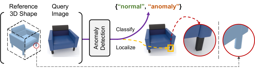
Motivated by the intuition above, this paper introduces a novel conditional AD task, along with a new benchmark and an effective solution, that aims to identify and localize anomalies from a photo of an object instance (i.e., the query image), in relation to a reference 3D model (see Fig. 1). The 3D model provides the reference shape for the regular object instance, and hence a clear definition of regularity for the query image. This setting is motivated by real-world applications in inspection and quality control, where an object instance is manufactured based on a reference 3D model, which can then be used to identify anomalies (e.g., production faults, damages) from a photo of the instance.
The proposed task goes beyond the single image analysis in standard AD benchmarks and requires the detection of subtle anomalies in shape by comparing two modalities, an image with its reference 3D model, which is challenging for three reasons. First, we would like our model to detect anomalies in previously unseen object instances from image-shape pairs at test time. Generalizing to unseen instances demands learning rich representations encoding a diverse set of 3D shapes and appearances while enabling accurate localization of anomalies. Second, the reference 3D model contains only shape but not texture information to simulate a realistic scenario where the 3D model can be used to produce instances with different materials, colors, and textures. The resulting domain gap between two modalities requires learning representations that are invariant to such appearance changes and sensitive to variations in geometry. Finally, in our benchmark, the viewpoint of the object instances in query images is not available in training. This requires the model to establish the local correspondences between the modalities, i.e., corresponding 3D location for each image patch in an unsupervised manner.
To tackle the first challenge, we propose a new large-scale dataset, BrokenChairs-180K, consisting of around 180 query images with diverse anomalies, geometries, and textures paired with 8,143 reference 3D shapes. Training on such a diverse dataset enables learning rich multi-modal representations to generalize to unseen objects. To address the domain gap between the query images and reference shapes, we follow two strategies. First, we render each reference shape from multiple viewpoints to generate a set of multi-view images to represent the 3D shape and use them as input along with a query image to our model. The multi-view representation facilitates learning domain-invariant representations through sharing the same encoder across query and multi-view images. Second, our model, Correspondence Matching Transformer (CMT) learns to capture cross-modality relationships by applying a novel cross-attention mechanism through a sparse set of local correspondences. Finally, to address the third challenge, we use an auxiliary task that forces the model to learn viewpoint invariant representations for each local patch in query and multi-view images enabling our method to align local features corresponding to the same 3D location regardless of its viewpoint without ground truth correspondences.
In summary, our main contributions are threefold, introducing a novel AD task, a large-scale benchmark to provide a testbed for future research, and a customized solution. Our model includes multiple technical innovations including a hybrid 2D-3D representation for 3D shapes, a transformer-based architecture that jointly learns to densely align query and multi-view images from image-level supervision and detect anomalies. Our results in extensive ablation studies clearly demonstrate that 3D information along with correspondence matching yields significant improvements. We also perform an additional perceptual study that evaluates the human performance on the task, showing that the proposed task is challenging. Finally, we evaluate our technique on real images showing promising results.
2 Related Work
AD methods. We refer to [9, 26] for detailed literature reviews. Unlike the standard AD techniques, we focus on a conditional and multi-modal AD problem which requires a joint analysis of a query image with a reference 3D shape to detect local irregularities in the image.
Conditional/referential AD. In many AD applications, the anomaly of an instance depends on its specific context [32]. For instance, anomalous temperature changes can be more accurately detected in a particular spatial and temporal context. We also study a specific application of the conditional AD problem where the context information is instance-specific and comes from a reference 3D shape.
AD image benchmarks. A major problem in the development of AD is the lack of large datasets with realistic anomalies. For semantic anomalies, a common practice (e.g., [7, 30]) is to select an arbitrary subset of classes from an existing classification dataset (e.g., MNIST [20], CIFAR10 [18]), treat them as an anomalous class, and train a model only on the remaining classes. There also exist multiple datasets that contain real-world anomalous instances including irregularly shaped objects [31], objects with various defects such as scratches, dents, contaminations [3], various defects in nanofibrous material [6] which focus on one sample at a time. A concurrent work, PAD [38] targets a similar objective with ours, while our task has fewer assumptions and is designed to detect fine-grained geometrical anomalies. Moreover, compared to the PAD dataset consisting of only 20 LEGO bricks of animal toys, ours comprises a large-scale collection of realistic chairs with diverse geometries, textures, and a wider range of fine-grained anomalies.
2D-3D cross-modal correlation. Image-based 3D shape retrieval [13, 14, 23] is a related problem that aims to retrieve the most similar shape for a given 2D image. Most existing works learn to embed 2D images and 3D shapes into a common feature space and perform metric learning using a triplet loss. Different to the retrieval task that primarily involves global-level matching, our focus is comprehending the correlation of fine-grained local details between the shape and the image to detect anomalies within the image. Another related area focuses on learning of 2D-3D correspondences [12, 28, 36, 21] by matching 2D and 3D locally with a triplet loss [12, 28], matching images and point clouds with a coarse-to-fine approach [21], improving matching robustness using a global-to-local Graph Neural Network [36]. 2D-3D correlation is also studied for specific applications such as object pose estimation [22, 37], 3D shape estimation [15] and object detection in images by using a set of 3D models [2]. Unlike the methods discussed here, our objective is to identify and localize anomalies in a given 2D query image in relation to a reference 3D model.
3 Building BrokenChairs-180K Dataset
To the best of our knowledge, there is no prior large public dataset with paired 3D shapes and images. Hence we introduce BrokenChairs-180K, a new benchmark for the proposed conditional AD task. Our dataset focuses on generating samples from one category, namely ‘chair’, which includes various subcategories like sofas, office chairs, and stools, while our generation pipeline is general and applicable to other categories. We picked this category as chairs contain a very wide range of shapes, appearances, and material combinations making them appealing for our experiments. In the following, we describe the generation procedure, including anomaly creation and realistic image rendering. More details can be found in the supplementary.
3.1 Creating Anomaly from 3D Objects
3D shape collection. To cover a wide variety of fine-grained anomalies across various parts of chairs (e.g., leg, arm, and headrest), we strive to collect 3D shapes that come with part annotations and thus opt to utilize the PartNet [25] as our starting point. PartNet is a large-scale dataset of 3D objects annotated with fine-grained part labels. Its chair category is among the most populous, providing a rich source of 3D shapes for our task. In particular, we use 8,143 3D chair shapes from PartNet. Given a 3D model of a chair and its part annotation, we automatically create anomalies by applying geometric deformations as described below.
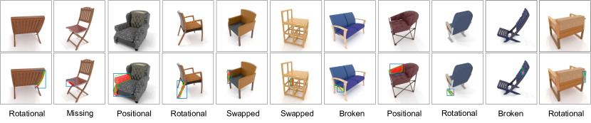
Generation of anomaly shapes. Our dataset covers five anomaly scenarios (see Fig. 2) relevant to real-world applications. (1) Positional anomalies pertain to deviations from the designated position of chair parts. To create a positional anomaly, we randomly select a part from a normal 3D model and apply random translation. (2) Rotational anomalies are created by applying a 3D rotational transformation to a randomly selected 3D part. (3) Broken or damaged parts consist cases that structural components are broken or damaged. We synthetically generate breaks using Boolean subtraction following [19] where we fracture a chair part by subtracting a random spherical or cubical geometric primitive from the part mesh. (4) Component swapping involves swapping common parts across different chair instances (e.g., ‘back-connector’ of one chair is exchanged with a ‘back-connector’ from another chair), simulating an incorrect assembly during manufacturing. (5) Missing components involve randomly choosing one part and removing it from the 3D shape. Next, we discuss the generation of query images with photo-realistic texture.
| Different types of Anomalies | |||||||
|---|---|---|---|---|---|---|---|
| Position | Rotation | Broken | Swapped | Missing | #Anomaly | #Normal | |
| #Shapes | 5,646 | 5,551 | 6,113 | 6,427 | 5,182 | 28,919 | 8,143 |
| #Images | 20,023 | 20,017 | 20,008 | 20,010 | 20,023 | 100,076 | 77,994 |
| #Views | [1,7,4] | [1,7,4] | [1,5,4] | [1,7,4] | [1,8,4] | [1,8,4] | [1,12,8] |
3.2 Photo-realistic Rendering of 3D objects
Assigning materials to 3D shapes. The shapes in PartNet only contain basic textures but no realistic materials. To enable realistic rendering, we use photo-realistic relightable materials from [27] represented as SVBRDF. In total, we utilize 400 publicly available SVBRDF materials, encompassing various types such as wood, plastic, leather, fabric, and metal. Following PhotoShape [27], we automatically assign a material to each semantic part of a 3D shape, and use Blender’s “Smart UV projection” algorithm to estimate the UV maps needed for texturing.
Rendering and view selection. We render each shape from various viewpoints sampled from a hemisphere around the object. The viewpoint is parameterized in spherical coordinates where azimuth values are sampled uniformly over with an interval of and elevation values are uniformly sampled in . The radius is fixed at for all views. For anomaly shapes, we only keep the rendering if the anomalous part is visible from the camera view. We employ a quality control and verification step (see supplementary) to discard bad-quality samples.
Dataset Statistics. Our dataset comprises a total of 8,143 reference 3D shapes (normal), along with around 180 images rendered at a resolution of pixels. Among these images, 100 contains anomalies, while the remaining are categorized as normal. Since in our solution, we use textureless multi-view images to represent the reference 3D shape, we further provide grayscale multi-view images111In practice, we clone grayscale values and convert each view to a three-channel image before feeding them as input to our model. rendered from 20 regularly sampled viewpoints for each reference shape. However, the 3D representation is not necessary to be multi-view images, alternative representations like mesh, point cloud, or voxel can be obtained from the reference shape and adopted by future algorithms when solving the conditional AD problem.
A detailed breakdown of these statistics is provided in Tab. 1. We divided the dataset into three distinct sets: 138 images for training, 13 for validation, and 26 for testing. Each set contains rendered images from a set of mutually exclusive 3D shapes. Hence, the evaluation is performed on previously unseen 3D shapes. Our dataset also contains bounding box and segmentation mask, localizing any anomalous region.
4 Proposed Method
4.1 Overview
Let be an dimensional RGB image of an object captured from an unknown viewpoint and be a set of dimensional images that are rendered from the reference shape at regularly sampled viewpoints on a hemisphere. We assume the model has access to the camera pose and depth map of each multi-view image. We wish to learn a classifier that takes in and and predicts the ground-truth binary anomaly label . Given a labeled training set including query, multi-view, and label triplets , the classifier can be optimized by minimizing the loss term:
| (1) |
where is the binary cross-entropy loss function.
An ideal classifier must identify subtle shape irregularities in by finding the relevant patches in for each patch in and comparing them. One straightforward design to relate patches across query and multi-view images is to use the cross-attention module [34]. In particular, one can use local features extracted from as query and ones from as key and value matrices as input to the scaled dot-product attention in [34] to cross-correlate them while predicting the anomaly label. While this design can implicitly capture such cross-correlations between patches from only image-level supervision when trained with the loss in Eq. 1, it fails to perform better than a similar model that is trained only on the query images in practice (see Sec. 5). We posit that the failure to utilize is due to the difficulty in establishing the correct correspondences from noisy correlations between all patches pairs across query and multi-view images only from image-level supervision.
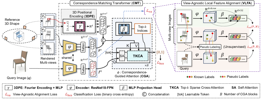
To address this challenge, we propose a new model, correspondence matching transformer (CMT) that consists of a CNN encoder, a 3D positional encoding (3DPE) module, a correspondence-guided attention (CGA) network, and lastly a view-agnostic local feature alignment (VLFA) mechanism (see Fig. 3). While the 3DPE module encodes the 3D location of the patches in multi-view images and facilitates finding local correspondences across views, the CGA network selectively conditions the final prediction on a small subset of the most related patches from multi-view images through a top-k sparse cross-attention (TKCA) mechanism. Finally, VLFA provides a richer supervision signal to establish correspondences between similar regions in the query and the multi-view images by using semi-supervised learning. Next, we describe them in detail.
4.2 Correspondence Matching Transformer
CMT uses ResNet18 feature pyramid network [24] as the feature encoder, which is denoted as where the input is down-scaled 8 times through the network ( and ). Once we extract the features of and for each , and respectively, we reshape each of them to be dimensional matrices, denote them as and respectively, where . Each column in and corresponds to a dimensional local feature. We use notation to indicate -th local feature or patch encoding, as each encoding approximately corresponds to a local patch in the input image due to locality in the convolutional encoder. Next, we describe key components of the CMT including the 3DPE and CGA modules.
3D Positional Encoding (3DPE).
While the multi-view representation allows for a simple and efficient model design through a shared feature encoder for our task, it also makes 3D information less accessible and hence hampers relating local features across different views accurately. To mitigate this problem, we propose complementing the multi-view images with 3D information. For each patch encoding , we first locate the corresponding image patch in and then compute the 3D position of the corresponding patch in the world coordinates 3D using the known camera parameters and depth maps. Then we use Fourier encoding to obtain a higher-dimensional vector for each and further process it through an MLP block to obtain a dimensional 3DPE. Formally, we denote the joint mapping by .
Compared to the 2D standard positional encoding used in transformer models [11], 3DPE encodes 3D object geometry in the world space. For each including patch encodings, we compute a corresponding dimensional matrix . For the next steps, we gather and over views, and concatenate each set along their second dimensions, resulting in and respectively where . Augmenting with results in a novel hybrid 2D-3D representation by incorporating explicit 3D information into the 2D multi-view images.
Correspondence-Guided Attention (CGA).
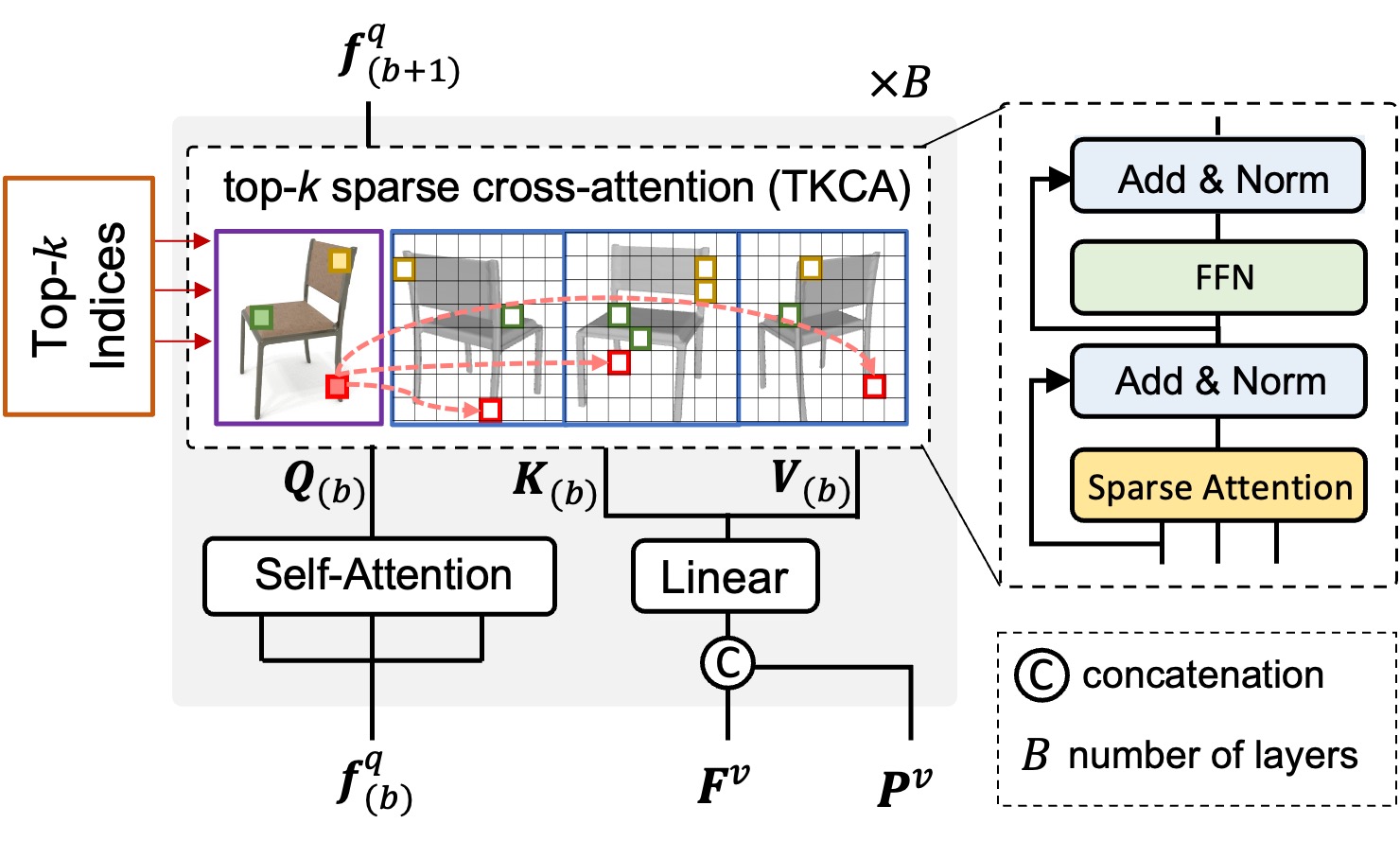
The CGA network , as illustrated in Fig. 4, takes in , , and predicts the anomaly label while efficiently computing the correlations across two modalities. CGA comprises consecutive transformer blocks where each block contains multiple operations and is indexed by subscript . In particular, the block starts with concatenating and along their first dimension, then the resulting dimensional matrix is reduced to dimensional matrix through a linear projection layer (Eq. 2). After self-attention operation (SA) is applied to the query features where (Eq. 3), it computes the query (Eq. 4) and key-value matrices , (Eq. 5) by applying the linear projections respectively.
| (2) | ||||
| (3) | ||||
| (4) | ||||
| (5) | ||||
| (6) | ||||
| (7) | ||||
| (8) | ||||
| (9) | ||||
Next, we pass to our top-k sparse cross-attention (TKCA) module (see Eq. 6). Unlike the vanilla cross-attention module in standard transformers [34, 11] ingesting all tokens for the attention computation, which is inefficient for our task and may introduce noisy interactions with irrelevant features, potentially degrading performance, TKCA calculates the attention between query and only a small subset of relevant multi-view features using a similarity matrix :
| (10) |
where is given by:
| (11) |
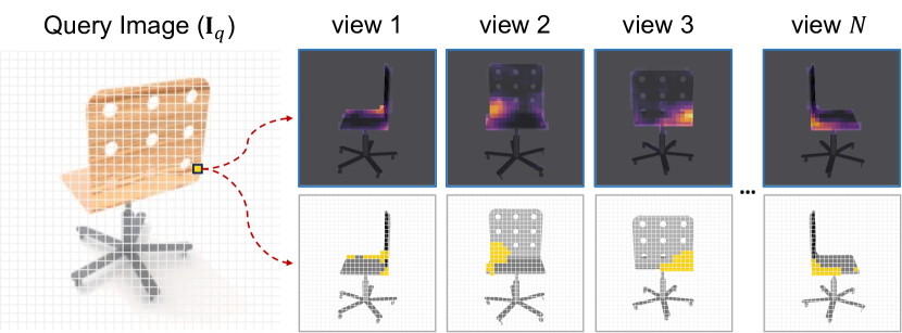
where operation selects the most similar features from multi-view representation (see Fig. 5) for -th query feature. To compute , we use an auxiliary function , instantiated as a four layered MLP followed by a final channel-wise normalization, that projects and each view in to a view-agnostic feature space where images corresponding to same object part in 3D has similar representations regardless of their viewpoint. To obtain the similarity between the query and multi-view patches, we compute the dot product between their projected features:
| (12) |
In contrast to other transformer architectures using sparse attention [35], TCKA chooses the top- elements based on a different source of information, geometric correspondences computed across two modalities, and enables an efficient computation of the cross-attention, as the same is used throughout the transformer blocks.
After the cross-correlation, the standard residual addition, normalization and feedforward (FFN) layers are applied to obtain as input to the next block (Eqs. 7, 8 and 9). Note that we use multiple heads, concatenate the outputs from multi-head attention and then derive the final attention results through linear projection. We append a learnable token denoted as [tok] to construct the query inputs of the CGA network. Through the transformer blocks, the output state of the [tok] token develops a consolidated representation enriched by learned shape-image correlation, which is used as input to the classification head.
4.3 View-Agnostic Local Feature Alignment
As discussed above, image-level supervision alone is too weak to capture fine localized correlations between and . Thus, we introduce an auxiliary task, VLFA that aims to densely align corresponding parts between query images and related views. Through , we learn to map and to a view-agnostic space such that their local features corresponding to the same object part are mapped to a similar point regardless of the viewpoint from which the image is captured. As the viewpoint of is unknown, the ground-truth correspondences between query and reference views cannot be obtained through inverse rendering.
To this end, we use a self-labeling strategy to generate pseudo-correspondences by finding the most similar local feature in the reference view to each local feature in the query at each training step, after mapping their features to the view-invariant space and normalizing them:
| (13) |
where and . We compute the pseudo-label for each and store them in a look-up table . In another one , we store the remaining set of reference view and index values that are not the corresponding location. Then, using as positive and negative correspondences respectively, we minimize a contrastive loss over each - pair:
| (14) |
where is a temperature parameter and . Due to the cost of computing the pseudo-correspondences for all query features across all views, we compute them only for a random subset of query features across randomly sampled views at each training iteration.
Learning correspondences through self-learning alone in the presence of the domain gap between query and reference views is a noisy process. Hence, we also exploit the known viewpoints of the multi-view images by densely aligning their local features in each view pair after computing the ground truth dense correspondences between them and discarding the ones that are occluded in one of the views. The key assumption here is that aligning different views by using their ground truth labels enables a more accurate correspondence learning between query images and views, as the parameters of the projection are shared across two domains. As before, we form two look-up tables and to store the positive and negative correspondences between two views, and randomly subsample them. After mapping them to the view-invariant space and normalizing them, we compute and minimize Eq. 14 for the pairs in the look-up tables.
The objective in Eq. 1 can be rewritten as:
| (15) |
where and are the alignment loss functions over query-view pairs and view-view pairs respectively, is a loss balancing weight set to .
5 Experiments
Implementation Details: The encoder takes a image as input and returns a feature block. Within the CGA network, we employ three transformer blocks (), and each applies 8-headed attention. The value of in TCKA is set to . During training, we randomly select a subset of views, and during testing, we utilize all 20 views. We apply basic data augmentation to the query images, which includes random horizontal flips and random cropping of regions, followed by resizing the cropped regions back to the original size of . We train our model for 20 epochs using 4 Titan RTX GPUs, maintaining a batch size of 8 in each GPU, and use the Adam optimizer with a learning rate of . We refer to the supplementary for more details.
5.1 Results
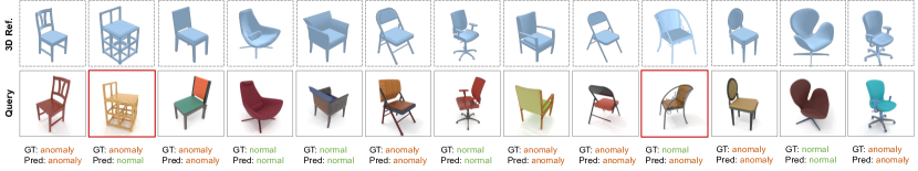
Since there is no related public benchmark for our task, we define several challenging baselines to evaluate our CMT. We report the quantitative results using two evaluation metrics – the area under the ROC curve (AUC) and accuracy in Tab. 2, and provide qualitative results in Fig. 6.
Importance of 3D reference shape. To assess the significance of using the reference shape, we establish baselines that solely rely on the query image for detecting anomalies. As our first baseline, we use a ResNet18-FPN model that takes in only query images as input. For the next two baselines, we add three self-attention blocks to ResNet18-FPN and use a ViT [11] respectively. Tab. 2 shows that the reference 3D shape is crucial to good performance while CMT outperforms the baselines by more than 10% in accuracy.
| 3D Ref. | Methods | AUC () | Accuracy () |
| ✗ | ResNet18-FPN [24] | 74.6 | 64.7 |
| ResNet18-FPN w/ SA blocks | 75.2 | 65.1 | |
| Vision Transformer (ViT) [11] | 75.4 | 65.2 | |
| ✓ | LFD [CVPR’19] [14] | - | 64.9 |
| Lin et al. [ICCV’21] [23] | - | 67.8 | |
| A: CMT (w/o CGA, VLFA, 3DPE) | 76.1 | 66.8 | |
| B: CMT (w/o VLFA, 3DPE) | 76.3 | 67.1 | |
| C: CMT (w/o CGA, 3DPE) | 80.8 | 72.3 | |
| D: CMT (w/o 3DPE) | 82.6 | 73.7 | |
| Ours: CMT | 84.7 | 75.4 |
| AUC () | Accuracy () | ||
|---|---|---|---|
| ✗ | ✗ | 78.5 | 68.3 |
| ✗ | ✓ | 78.6 | 68.1 |
| ✓ | ✗ | 81.6 | 73.7 |
| ✓ | ✓ | 84.7 | 75.4 |
Comparison with related work. As there is no prior work designed for our problem, we take two recent image-based 3D shape retrieval techniques [14, 23] that learn to embed 2D images and 3D shapes into a common feature space and perform metric learning using a triplet loss. Once we train them in our dataset, we evaluate them by using the distance between the query and reference shape embeddings to obtain the classification score after a thresholding step. Based on results in Tab. 2, we argue that these methods fail to locate subtle variations in geometry, as the cross-modal correlations are only learned at the image level missing fine-grained local correspondence learning.
Ablation of CGA, VLFA and 3DPE. Our first baseline (A) includes none of the three components but a standard cross-attention module to relate two modalities using all local patches. Surprisingly, A obtains only a 1.6% accuracy improvement over the query-only baseline, indicating its inability to fully leverage the reference shape. Baseline B includes only the CGA component with the top- sparse cross-attention, baseline C, contains the VLFA but with a standard cross-attention. While baseline B does not show much improvement over A, baseline C performs significantly better than A obtaining a 5.2% accuracy gain. This clearly demonstrates the importance of the auxiliary task where we learn matching correspondences for the AD task and that the CGA fails to acquire meaningful correspondences in the absence of the VLFA. Baseline D that employs both CGA and VLFA further boosts the performance of C through its selective sparse attention mechanism. Finally, our model, which includes all the components, outperforms D thanks to the introduction of 3DPE that facilitates corresponding matching across different views.
Ablation of loss functions. Tab. 3 reports an ablation study on the loss functions used for learning the view-agnostic representation. Utilizing only query-view alignment loss () does not yield any advantages (row 2) over not employing any alignment loss (row 1). However, employing the view-view alignment () alone leads to improved results (row 3). The optimal result is achieved when both components are combined (row 4).
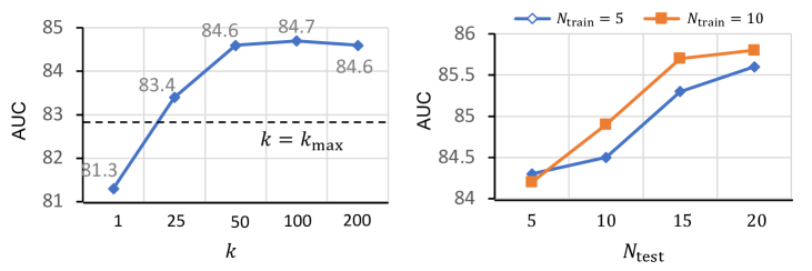
Sensitivity to . We analyze the performance under different values of in Fig. 7 (left). Compared to the maximum possible that is , we analyze significantly smaller values and, among them, show yields the best result. Using all available tokens results in deteriorated performance (shown as the dotted horizontal line) showing that our top- sparse attention is effective in eliminating the noisy patches by using only the top-related ones.
Sensitivity to . Fig. 7 (right) depicts the analysis on the number of input views for training and testing, and respectively. To this end, we train two separate CMT models with 5 and 10 views, and evaluate each using 5, 10, 15, and 20 views at test time. The plot shows that, while increasing views in both training and testing helps, training with few views and testing on more views can provide a good tradeoff between training time and performance.
Viewpoint prediction. As a side product of establishing the correspondences across the query image and views in our model, we could estimate the camera viewpoint in the query image w.r.t. a reference shape. To this end, we compute dense correspondences between the query image and each view image, and then calculate the distance between the pixel coordinates of each point in the query image and their predicted correspondences in the multi-view images, and choose the view with the lowest average distance as the approximate viewpoint. As a baseline, we train a ResNet with the viewpoint supervision on the normal images only, and evaluate it on the test normal query images. Our model, trained with no viewpoint supervision, achieves a significantly better accuracy (47% vs 89%) when predicting the closest view suggesting that our model implicitly learns to relate the query image with the closest views.
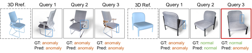
Evaluation on real data. Here we apply our model, which is trained on the synthetic BrokenChairs-180K dataset, on a small set of real chair samples that contain multiple pairs of the reference 3D shape, query images containing either normal or irregular instances with broken, removed, or misaligned parts from various viewpoints. Background pixels in query images are removed by using a segmentation method [17] in a preprocessing step and also a synthetic shadow was added to match the training images. To obtain the reference 3D shapes, we take multiple photos of object instances while walking around them, use the 3D reconstruction software [33], and finally apply Laplacian smoothing to post-process it. Fig. 8 illustrates the results for two regular reference shapes, each paired with three query images. In 5 out of 6 cases, our method successfully classifies and localizes the anomalous parts, while in the failure case, it incorrectly relates the self-occluded arm with an anomaly.
Anomaly localization. Here we adopt our model to localize anomalies in the form of a bounding box, use a bounding box regression head (a 4-layer MLP), and jointly train it with the other network parameters by using L1 regression and generalized IoU loss [29]. This model achieves 56.5% average precision on our dataset, outperforms a ViT baseline that is trained only on the query images, and obtains 42.6%. Moreover, jointly learning the classification and localization further boosts the classification performance to 85.9 (+1.2) AUC and 77.3% (+1.9) accuracy.
User Perceptual Study. We also evaluated human performance in our task and conducted a study with 100 participants. We presented each participant with 10 pairs of reference shapes and query images, with each pair randomly selected from a random subset of 200. We observe a human accuracy of 70.6%, showing that the proposed task is challenging, while our CMT obtains a superior accuracy of 74.8% on the same subset.
6 Conclusion
In this paper, we have introduced a new AD task, a new benchmark, and a customized solution inspired by quality control and inspection scenarios in manufacturing. We showed that an accurate detection of fine-grained anomalies in geometry requires a careful study of both modalities jointly. Our method achieves this goal by learning dense correspondence across those modalities from limited supervision. Our benchmark and method also have limitations. Due to the difficulty and cost of obtaining real damaged objects, our dataset contains only shapes and images of synthetic objects and currently is limited to a single yet very diverse category of ‘chair’, presence of only one anomaly in each query image, focusing only on shape anomalies excluding the appearance based ones such as fading, discolor, texture anomaly. Moreover, our model assumes that object instances are rigid, and cannot deal with articulations and deformations, and requires an accurate reference 3D shape for accurate detection.
References
- Ahmed and Courville [2020] Faruk Ahmed and Aaron Courville. Detecting semantic anomalies. In AAAI, 2020.
- Aubry et al. [2014] Mathieu Aubry, Daniel Maturana, Alexei A Efros, Bryan C Russell, and Josef Sivic. Seeing 3d chairs: exemplar part-based 2d-3d alignment using a large dataset of cad models. In CVPR, 2014.
- Bergmann et al. [2019] Paul Bergmann, Michael Fauser, David Sattlegger, and Carsten Steger. Mvtec ad–a comprehensive real-world dataset for unsupervised anomaly detection. In CVPR, 2019.
- Bergmann et al. [2021] Paul Bergmann, Kilian Batzner, Michael Fauser, David Sattlegger, and Carsten Steger. The mvtec anomaly detection dataset: a comprehensive real-world dataset for unsupervised anomaly detection. IJCV, 2021.
- Blum et al. [2021] Hermann Blum, Paul-Edouard Sarlin, Juan Nieto, Roland Siegwart, and Cesar Cadena. The fishyscapes benchmark: Measuring blind spots in semantic segmentation. IJCV, 2021.
- Carrera et al. [2016] Diego Carrera, Fabio Manganini, Giacomo Boracchi, and Ettore Lanzarone. Defect detection in sem images of nanofibrous materials. IEEE Transactions on Industrial Informatics, 2016.
- Chalapathy et al. [2018] Raghavendra Chalapathy, Aditya Krishna Menon, and Sanjay Chawla. Anomaly detection using one-class neural networks. arXiv preprint arXiv:1802.06360, 2018.
- Chan et al. [2021] Robin Chan, Krzysztof Lis, Svenja Uhlemeyer, Hermann Blum, Sina Honari, Roland Siegwart, Pascal Fua, Mathieu Salzmann, and Matthias Rottmann. Segmentmeifyoucan: A benchmark for anomaly segmentation. arXiv preprint arXiv:2104.14812, 2021.
- Chandola et al. [2009] Varun Chandola, Arindam Banerjee, and Vipin Kumar. Anomaly detection: A survey. ACM computing surveys, 2009.
- Deecke et al. [2021] Lucas Deecke, Lukas Ruff, Robert A Vandermeulen, and Hakan Bilen. Transfer-based semantic anomaly detection. In ICML, 2021.
- Dosovitskiy et al. [2021] Alexey Dosovitskiy, Lucas Beyer, Alexander Kolesnikov, Dirk Weissenborn, Xiaohua Zhai, Thomas Unterthiner, Mostafa Dehghani, Matthias Minderer, Georg Heigold, Sylvain Gelly, et al. An image is worth 16x16 words: Transformers for image recognition at scale. In ICLR, 2021.
- Feng et al. [2019] Mengdan Feng, Sixing Hu, Marcelo H Ang, and Gim Hee Lee. 2d3d-matchnet: Learning to match keypoints across 2d image and 3d point cloud. In ICRA, 2019.
- Grabner et al. [2018] Alexander Grabner, Peter M Roth, and Vincent Lepetit. 3d pose estimation and 3d model retrieval for objects in the wild. In CVPR, 2018.
- Grabner et al. [2019] Alexander Grabner, Peter M Roth, and Vincent Lepetit. Location field descriptors: Single image 3d model retrieval in the wild. In 3DV, 2019.
- Hejrati and Ramanan [2012] Mohsen Hejrati and Deva Ramanan. Analyzing 3d objects in cluttered images. NeurIPS, 2012.
- Hendrycks and Gimpel [2017] Dan Hendrycks and Kevin Gimpel. A baseline for detecting misclassified and out-of-distribution examples in neural networks. In ICLR, 2017.
- Kirillov et al. [2023] Alexander Kirillov, Eric Mintun, Nikhila Ravi, Hanzi Mao, Chloe Rolland, Laura Gustafson, Tete Xiao, Spencer Whitehead, Alexander C Berg, Wan-Yen Lo, et al. Segment anything. arXiv preprint arXiv:2304.02643, 2023.
- Krizhevsky and Hinton [2009] Alex Krizhevsky and Geoffrey Hinton. Learning multiple layers of features from tiny images. 2009.
- Lamb et al. [2022] Nikolas Lamb, Sean Banerjee, and Natasha Kholgade Banerjee. Deepjoin: Learning a joint occupancy, signed distance, and normal field function for shape repair. In ACM TOG, 2022.
- LeCun et al. [1998] Yann LeCun, Léon Bottou, Yoshua Bengio, and Patrick Haffner. Gradient-based learning applied to document recognition. Proceedings of the IEEE, 1998.
- Li et al. [2023] Minhao Li, Zheng Qin, Zhirui Gao, Renjiao Yi, Chenyang Zhu, Yulan Guo, and Kai Xu. 2d3d-matr: 2d-3d matching transformer for detection-free registration between images and point clouds. In ICCV, 2023.
- Lim et al. [2013] Joseph J Lim, Hamed Pirsiavash, and Antonio Torralba. Parsing ikea objects: Fine pose estimation. In ICCV, 2013.
- Lin et al. [2021] Ming-Xian Lin, Jie Yang, He Wang, Yu-Kun Lai, Rongfei Jia, Binqiang Zhao, and Lin Gao. Single image 3d shape retrieval via cross-modal instance and category contrastive learning. In ICCV, 2021.
- Lin et al. [2017] Tsung-Yi Lin, Piotr Dollar, Ross Girshick, Kaiming He, Bharath Hariharan, and Serge Belongie. Feature pyramid networks for object detection. In CVPR, 2017.
- Mo et al. [2019] Kaichun Mo, Shilin Zhu, Angel X Chang, Li Yi, Subarna Tripathi, Leonidas J Guibas, and Hao Su. Partnet: A large-scale benchmark for fine-grained and hierarchical part-level 3d object understanding. In CVPR, 2019.
- Pang et al. [2021] Guansong Pang, Chunhua Shen, Longbing Cao, and Anton Van Den Hengel. Deep learning for anomaly detection: A review. ACM computing surveys, 2021.
- Park et al. [2018] Keunhong Park, Konstantinos Rematas, Ali Farhadi, and Steven M Seitz. Photoshape: Photorealistic materials for large-scale shape collections. In SIGGRAPH Asia, 2018.
- Pham et al. [2020] Quang-Hieu Pham, Mikaela Angelina Uy, Binh-Son Hua, Duc Thanh Nguyen, Gemma Roig, and Sai-Kit Yeung. Lcd: Learned cross-domain descriptors for 2d-3d matching. In AAAI, 2020.
- Rezatofighi et al. [2019] Hamid Rezatofighi, Nathan Tsoi, JunYoung Gwak, Amir Sadeghian, Ian Reid, and Silvio Savarese. Generalized intersection over union: A metric and a loss for bounding box regression. In CVPR, 2019.
- Ruff et al. [2018] Lukas Ruff, Robert Vandermeulen, Nico Goernitz, Lucas Deecke, Shoaib Ahmed Siddiqui, Alexander Binder, Emmanuel Müller, and Marius Kloft. Deep one-class classification. In ICML, 2018.
- Saleh et al. [2013] Babak Saleh, Ali Farhadi, and Ahmed Elgammal. Object-centric anomaly detection by attribute-based reasoning. In CVPR, 2013.
- Song et al. [2007] Xiuyao Song, Mingxi Wu, Christopher Jermaine, and Sanjay Ranka. Conditional anomaly detection. IEEE TKDE, 2007.
- Tancik et al. [2023] Matthew Tancik, Ethan Weber, Evonne Ng, Ruilong Li, Brent Yi, Terrance Wang, Alexander Kristoffersen, Jake Austin, Kamyar Salahi, Abhik Ahuja, et al. Nerfstudio: A modular framework for neural radiance field development. In ACM SIGGRAPH, 2023.
- Vaswani et al. [2017] Ashish Vaswani, Noam Shazeer, Niki Parmar, Jakob Uszkoreit, Llion Jones, Aidan N Gomez, Łukasz Kaiser, and Illia Polosukhin. Attention is all you need. In NeurIPS, 2017.
- Wang et al. [2022] Pichao Wang, Xue Wang, Fan Wang, Ming Lin, Shuning Chang, Hao Li, and Rong Jin. Kvt: k-nn attention for boosting vision transformers. In ECCV, 2022.
- Wang et al. [2023] Shuzhe Wang, Juho Kannala, and Daniel Barath. Dgc-gnn: Descriptor-free geometric-color graph neural network for 2d-3d matching. arXiv preprint arXiv:2306.12547, 2023.
- Xiao et al. [2012] Jianxiong Xiao, Bryan Russell, and Antonio Torralba. Localizing 3d cuboids in single-view images. NeurIPS, 2012.
- Zhou et al. [2024] Qiang Zhou, Weize Li, Lihan Jiang, Guoliang Wang, Guyue Zhou, Shanghang Zhang, and Hao Zhao. Pad: A dataset and benchmark for pose-agnostic anomaly detection. In NeurIPS, 2024.