A Novel Phase Diagram for a Spin-$1$ System Exhibiting a Haldane Phase

Abstract

We provide the phase diagram of a 2-parameter spin-1 chain that has a symmetry-protected topological (SPT) Haldane phase using computational algorithms along with tensor-network tools. We improve previous results, showing the existence of a new phase and new triple points. New striking features are the triple end of the Haldane phase and the complexity of phases bordering the Haldane phase in proximity—allowing moving to nearby non-SPT phases via small perturbations. These characteristics make the system, which appears in Rydberg excitons, e.g. in Cu₂O, a prime candidate for applications.

Introduction.—Topological phases of matter have drawn a lot of attention due to their remarkable properties. Their edge transport protection from disorder and imperfections offers intrinsic physical immunity to noise. This has found many applications in diverse areas like dissipationless electronics, spintronics, lasers, and quantum computing [1, 2, 3, 4, 5].

The modern framework for classifying phases of matter started with the Landau-Ginzburg paradigm, where phases were classified by symmetry breaking [6]. This picture was challenged by the discovery of the integer quantum Hall effect, the fractional quantum Hall effect [7, 8, 9], and subsequent models like topological insulators that do not require external magnetic fields [10], Haldane phase in 1D spin chains [11, 12], quantum spin Hall effect [13, 14], string-net models [15] and quantum double models [16]. These models exhibit phases that can not be distinguished locally, can occur at zero temperature, and have a finite energy gap above the ground state. They are collectively called topological quantum phases [17].

The now well-established paradigm of quantum phase transitions identifies two phases of gapped ground states if there exists an adiabatic path connecting their Hamiltonians without closing the finite energy gap and avoiding any singularity in the local properties of the ground state [18]. The topological quantum phases are then classified into three categories: intrinsic topological order which follows this definition without any additional requirements (the phase can not be adiabatically connected to any topologically trivial phase), symmetry-protected topological phases (SPT) which only obeys this definition if certain symmetries are imposed on this adiabatic path, and symmetry-enriched topological phases (SET) when the underlying system has intrinsic topological order and then the phases are enriched by imposing symmetries [19, 18].

In 1D, there are no phases with intrinsic topological order; it can be shown that any gapped phase with local Hamiltonian is adiabatically connected to the trivial phase when no symmetries are imposed [20]. Consequently, the only topological phases in 1D are SPT phases. SPT phases can have nontrivial edge states. These edge states can implement topological quantum computing similar to Majorana zero modes [1, 2, 3].

Haldane mapped the spin-$1$ antiferromagnetic Heisenberg chain exhibiting $SU(2)$ symmetry: ${H}_{\mathrm{Heisenberg}}=J\sum_{i}\mathbf{S}_{i}\cdot\mathbf{S}_{i+1}\text{ with }J>0$ to the topological quantum field theory of the nonlinear sigma model. He then conjectured that the system would be gapped in 1D chains with integer spin [12, 11]. This was counterintuitive, as the Bethe ansatz for the spin-$\frac{1}{2}$ case is gapless [21]. The AKLT model presented an exactly solvable model which retains the Heisenberg model’s full $SU(2)$ symmetry: $H_{\mathrm{AKLT}}=\sum_{i}\left[\frac{1}{2}\mathbf{S}_{i}\cdot\mathbf{S}_{i+1}+\frac{1}{6}\left(\mathbf{S}_{i}\cdot\mathbf{S}_{i+1}\right)^{2}+\frac{1}{3}\right]$. In the AKLT model, the existence of an energy gap, non-trivial entanglement spectrum, and edge states can be proved analytically [22]. It was later shown that the topological Haldane phase could be realized using only the $\mathbb{Z}_{2}\times\mathbb{Z}_{2}$ internal symmetry which is a subset of the $SU(2)$ symmetry [23]. This symmetry is represented by the $\pi$-rotations around $x$-axis and $y$-axis: $e^{i\pi S^{x}}$ and $e^{i\pi S^{y}}$. Under this symmetry, the Haldane phase belongs to the class of SPT phases [23].

We consider a more general spin-$1$ Hamiltonian which has $\mathbb{Z}_{2}\times\mathbb{Z}_{2}$ symmetry but only has $U(1)$ symmetry around the z-axis Eq. (1). Many important Hamiltonians like Heisenberg, AKLT, Ising, and XXZ are special cases of this Hamiltonian. The model exhibits the topologically nontrivial Haldane phase. It can be realized using a 1D chain of traps of Rydberg excitons in Cu₂O [24]. Previous studies left some questions open, like whether all phases meet at triple or higher critical points. They also suggest a direct phase transition from the ferromagnetic to the antiferromagnetic phase. We show that all critical points are triple points as shown in Fig. 2. Four of them involve the Haldane phase. Interestingly, there is a new direct phase transition between the Haldane phase and the anisotropic phase with magnetization in the $x$ or $y$ directions. This can be particularly useful because out-of-plane magnetization is usually easier to measure experimentally. We also predict the existence of a new phase we call the negative D phase obstructing direct phase transitions between the ferromagnetic and the antiferromagnetic phases.

$${H}= \sum_{i}c_{0}+(c_{1}+\delta c_{1})S_{i}^{z}S_{i+1}^{z}+c_{2}\left(S_{i}^{x}S_{i+1}^{x}+S_{i}^{y}S_{i+1}^{y}\right)+c_{3}\left(S_{i}^{z}S_{i+1}^{z}\right)^{2}+c_{4}\left(S_{i}^{x}S_{i+1}^{x}+S_{i}^{y}S_{i+1}^{y}\right)^{2}$$ (1)

$$+c_{5}\left[S_{i}^{z}S_{i+1}^{z}\left(S_{i}^{x}S_{i+1}^{x}+S_{i}^{y}S_{i+1}^{y}\right)+\left(S_{i}^{x}S_{i+1}^{x}+S_{i}^{y}S_{i+1}^{y}\right)S_{i}^{z}S_{i+1}^{z}\right]+c_{6}\left(S_{i}^{x}S_{i+1}^{y}-S_{i}^{y}S_{i+1}^{x}\right)^{2}+D\left[\left(S_{i}^{z}\right)^{2}-2/3\right].$$

Rydberg Excitons.—Rydberg atoms have an electron excited far from its valence shell leaving a hole behind. The pair then resembles a Hydrogen atom and exhibits long-range dipole-dipole interactions and robust Rydberg blockade [25]. Analogously, in a semiconductor, an electron can be excited from the filled valence band to the conduction band leaving a hole behind. This electron-hole pair is called an exciton [26]. Rydberg excitons trapped in a 1D chain in Cu₂O in their $l=1$ angular momentum states are symmetric under $U(1)$ rotations around the z-axis and under $\mathbb{Z}_{2}\times\mathbb{Z}_{2}$ reflections around x-axis and y-axis [27, 24]. We can then use them as a concrete realization of our Hamiltonian, Eq. (1).

Rydberg atoms and excitons were used in many applications [25, 28, 29, 30, 31]. In these applications, they were mostly used as two-level systems distinguishing the ground state from other excited states (qubits). However, our implementation here is different as we are exploiting the angular momentum degree of freedom which offers a richer structure that acts as an intrinsic spin-$1$ system (qutrit). This offers a more direct simulation platform for many-body systems with integer spin.

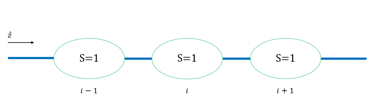
Figure 1: The 1D chain of spin-$1$ particles. Blue lines represent the interactions between nearest neighbors. The $z$-axis is aligned with the chain.

Model.— The model consists of a 1D chain of spin-$1$ particles with nearest-neighbor interactions Fig. 1. We further include two perturbations $D\left[\left(S_{i}^{z}\right)^{2}-2/3\right]$ and $\delta c_{1}S_{i}^{z}S_{i+1}^{z}$. These perturbations do not break the symmetries of the Hamiltonian Eq. (1). They correspond to trap anisotropy and coupling anisotropy in the excitons implementation [27, 24]. We fix the seven constants $c_{0}-c_{6}$ to match the Rydberg excitons in Cu₂O [27] as presented in Eq. 2.

$$\begin{array}[]{r@{}l r@{}l r@{}l r@{}l}c_{0}&=-5.58\epsilon_{0},&c_{1}&=9.53\epsilon_{0},&c_{2}&=-8.97\epsilon_{0},&c_{3}&=1.27\epsilon_{0},\\ c_{4}&=6.59\epsilon_{0},&c_{5}&=-3.18\epsilon_{0},&c_{6}&=5.04\epsilon_{0}.&&\end{array}$$ (2)

Here, $\epsilon_{0}=10^{-4}n^{11}\hbar\mathrm{s}^{-1}\times\mu\mathrm{m}^{6}/R^{6}$ where $n$ is the quantum number which ranges from 12 to 25, and $R$ is the distance between traps [27].

Order Parameters.— The model exhibits six phases: antiferromagnetic, ferromagnetic, anisotropic, Haldane, negative D, and large D phases. The anisotropic phase has magnetization in the XY plane. The last two phases are disordered phases having no magnetization or Néel order in any direction. For the magnetic phases, we use the antiferromagnetic order parameter: $\hat{O}_{\text{AFM}}=\lim_{|i-j|\to\infty}(-1)^{|i-j|}\langle S_{i}^{z}S_{j}^{z}\rangle$ and the ferromagnetic order parameter which is just the magnetization in the $z$-axis: $\langle{S_{z}}\rangle=\frac{\langle\sum_{i}S_{i}^{z}\rangle}{N}$. The anisotropic phase can be detected using the $S_{x}$ ferromagnetic order parameter: $\langle{S_{x}}\rangle=\frac{\langle\sum_{i}S_{i}^{x}\rangle}{N}$. We could also use a similar order parameter for $S_{y}$ since the anisotropic phase is degenerate in the XY plane, practically however, the DMRG algorithm usually picks the x-axis in a numerical spontaneous symmetry breaking. This can be confirmed by adding the slightest magnetization in the y-axis to the Hamiltonian which will make the system pick up magnetization in the y-direction instead. For the Haldane phase, we use the string order parameter [32]. More details on generalized string order parameters are provided in appendix B6:

$$\hat{O}_{\text{string}}=\lim_{|i-j|\to\infty}\langle S_{i}^{z}[\Pi_{k=i+1}^{j-1}e^{i\pi S_{k}^{z}}]S_{j}^{z}\rangle$$ (3)

It should be noted that the string order parameter will necessarily have a zero value for any trivial SPT phase only if the phase is symmetric. The string order parameter can have a non-zero value for a trivial SPT phase if the symmetry is broken. For example, the Néel state $\psi_{\text{ N\'{e}el}}=\ket{1}\otimes\ket{-1}\otimes\ket{1}\otimes\ket{-1}\otimes\cdots$ will have a non-zero value for the string order parameter but, that is because it breaks the $\mathbb{Z}_{2}\times\mathbb{Z}_{2}$ symmetry, namely the $e^{i\pi S_{x}}$ symmetry. This issue is resolved by first inspecting the symmetry-breaking phases and then classifying the symmetry-preserving phases using the topological order parameters. In our case, it is also convenient to combine order parameters to distinguish the Haldane phase from other topologically trivial phases using only one order parameter. We define:

$$\hat{O}_{\text{Adjusted String}}=a_{1}\hat{O}_{\text{String}}e^{-a_{2}|\hat{O}_{\text{AFM}}|}$$ (4)

for appropriate large constant $a_{2}$ and small $a_{1}$. This new order parameter will be non-zero in the Haldane phase and will decay exponentially in the antiferromagnetic phase. The new negative D phase is characterized by the absence of all order parameters except $\hat{O}_{S_{z}^{2}}$:

$$\hat{O}_{S_{z}^{2}}=\langle\left(S^{z}\right)^{2}\rangle=1$$ (5)

The large D phase is distinguished by the vanishing of all order parameters. These order parameters are then used to construct the full phase diagram Fig. 2 as summarized in Table 1.

Phase	Non-zero Order Parameter(s)	SPT
Antiferromagnetic	$\hat{O}_{\text{AFM}}$, $\hat{O}_{S_{z}^{2}}$ and $\hat{O}_{\text{String}}$	Trivial
Ferromagnetic	$\hat{S_{z}}$ and $\hat{O}_{S_{z}^{2}}$	Trivial
Anisotropic	$\hat{S_{x}}$, $\hat{O}_{S_{z}^{2}}$ and $\hat{S_{z}}$	Trivial
Haldane	$\hat{O}_{\text{String}}$, $\hat{O}_{\text{Adj. String}}$ and $\hat{O}_{S_{z}^{2}}$	Nontrivial
Negative D	$\hat{O}_{S_{z}^{2}}$	Trivial
Large D	None	Trivial

Table 1: Order Parameters for different Phases

We used the density matrix renormalization group (DMRG) algorithm to obtain the extended phase diagram for the finite system $N=100$ and the variational uniform matrix product states (VUMPS) algorithm to simulate the system in the infinite thermodynamic limit [33, 34, 35]. Both algorithms use matrix-product state (MPS) representation of the wave function [33, 36, 37]:

$$\ket{\psi}=\Tr(A^{p_{1}}A^{p_{2}}\cdots A^{p_{N}})\ket{p_{1}}\otimes\ket{p_{2}}\dots\otimes\ket{p_{N}}$$ (6)

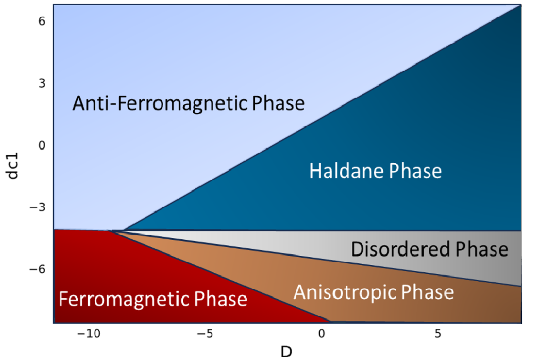
(a) The previous phase diagram calculated in [24].

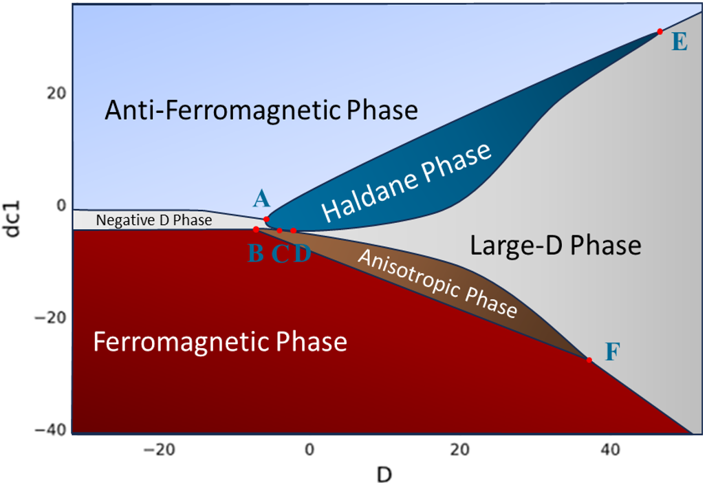
(b) The updated phase diagram showing the six triple points labeled by letters A-F.

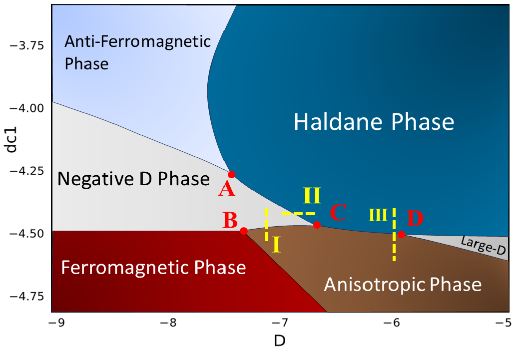
(c) The phase transitions used to prove the topology of the critical points.

Figure 2: Comparison of the old phase diagram (a), the updated phase diagram (b), and the close-up phase diagram (c) for the Hamiltonian Eq. (1) for different values of the trap anisotropy $D$ and coupling anisotropy $\delta c_{1}$.

This is a representation of a periodic and translational invariant state. The indices $p_{i}$ run over the spin-$1$ degrees of freedom. The matrices $A^{p_{i}}$ have dimensions $\chi\times\chi$ where $\chi$ is the bond dimension and it captures entanglement. The product state, for example, is represented by $\chi=1$; see see appendix A for more details. In DMRG calculations, we used bond dimensions up to $\chi=200$. In VUMPS calculations, we used a two-site unit cell and bond dimensions up to $\chi=300$. We achieved energy convergence of better than $0.1\%$ in both algorithms. Usually, the positions of the phase transitions are a little different from the finite to the infinite limit due to finite-size effects but, this did not affect the conclusions drawn about the topology of critical points.

Results.—The phase diagram of the model was first considered in [24] as presented in Fig. 2a. We obtained an updated phase diagram shown in Fig. 2b and a close-up of the central region is shown in Fig. 2c. There are six triple points $A-F$. Four of them are in contact with the Haldane phase. A new phase, which we call the negative D phase, appears in a narrow strip between the ferromagnetic and antiferromagnetic phases and extends as $D\to-\infty$.

Two important numerical results of the phase diagram are shown in Fig. 3. In Fig. 3a, the adjusted string order parameter: $\hat{O}_{\text{Adj. String}}=a_{1}\hat{O}_{\text{string}}e^{-a_{2}|\hat{O}_{\text{AF}}|}$ highlights the region hosting the topological Haldane phase. In Fig. 3b, we added the adjusted string and the ferromagnetic order parameters $\langle S_{z}\rangle$ and $\hat{O}_{\text{AFM}}$ to visualize the phases and critical points in the central region. Fig. 3b is then used to synthesize Fig. 2c.

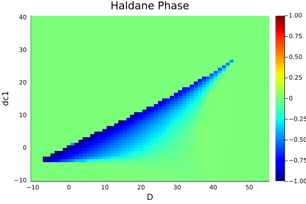
(a) Heat map of the adjusted string order parameter Eq. (4) which is only non-zero in Haldane phase. Here $(a_{1},a_{2})=(3,-20).$

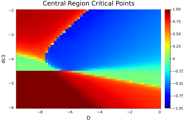
(b) Heat map of adjusted string order parameter defined with $(a_{1},a_{2})=(1,-20)$ and adding $\langle S_{z}\rangle$ and $\hat{O}_{\text{AFM}}$ .

Figure 3: (a) shows the asymptotic behavior of the Haldane phase while (b) shows the numerical data used to construct Fig. 2c.

Triple Points.—The existence of the triple points $A,B,C$, and $D$ can be proven by investigating direct phase transition before and after the triple points. This is achieved by studying three paths in the phase diagram shown in Fig. 2c. Fig. 4a shows line II where a direct transition from the negative D phase to the Haldane phase occurs. The vanishing of $\hat{O}_{\text{AFM}}$ throughout this path shows the termination of the antiferromagnetic phase after point $A$. Negative D phase has $\hat{O}_{S_{z}^{2}}=1$ which starts to decrease after the phase transition. Fig. 4b follows line III and shows a direct transition from the anisotropic phase with non-zero $\langle S_{x}\rangle$ to the Haldane phase.

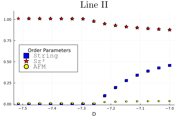
(a) Direct phase transition from Negative D phase to Haldane phase at $\delta c1=-4.35$.

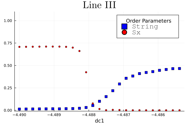
(b) The direct transition from Anisotropic phase to Haldane phase at $D=-6.2$

Figure 4: Proving the Existence of critical points $A-D$.

Asymptotic Behavior.—Upon extending the parameter space we discover that the Haldane and the anisotropic phases end with triple points $E$ and $F$ Fig. 2b. This is expected from the asymptotic behavior of the two parameters $D$ and $\delta c_{1}$. When $(D,\delta c_{1})\to(\infty,\infty)$, the model resembles an Ising Hamiltonian with uniaxial anisotropy $H\approx\sum_{i}c_{z}S_{i}^{z}S_{i+1}^{z}+D\left(S_{i}^{z}\right)^{2}$. In this regime, we expect only antiferromagnetic or large D phases. Similarly, when $(D,\delta c_{1})\to(\infty,-\infty)$, only ferromagnetic or large D phases will survive. The existence of the triple point $E$ is evidenced by a direct phase transition between the antiferromagnetic and large D phase at $\delta c_{1}=30$ proving that the Haldane phase ends Fig. 5. Analogously, the existence of triple point $F$ is proven by a direct transition from the ferromagnetic phase to the large D phase (not shown here).

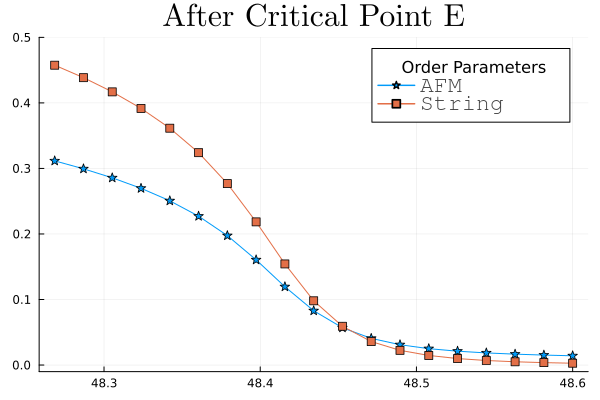
Figure 5: The simultaneous vanishing of both parameters shows a direct phase transition from the antiferromagnetic to the large D phase proving that Haldane phase terminates.

Outlook.—We constructed and analyzed the rich topological phase diagram for a spin-1 system hosting six different phases and six triple points. The effect of dimerization [38] or different trap geometries for Rydberg excitons [39, 40] is expected to exhibit exotic phenomena such as fifth-order transitions [41]. It would also be interesting to examine these new phase transitions using photoluminescence spectra of the exciton chain [42] to explore possible applications in the field of quantum simulations.

Acknowledgments.—The authors are grateful for the internal funding support from the College of Science at Purdue University. S.K. and S.C. would like to acknowledge the support from the Department of Energy, the Office of Science, and the Quantum Science Center (QSC).

Appendix A Matrix-Product States

Matrix-product states (MPS) representation plays a crucial role in representing 1D systems and offers the theoretical basis for efficient 1D algorithms like DMRG [33]. MPS is a representation of certain wave functions typically in 1D as:

$$\ket{\psi}=\Tr(A^{p_{1}}A^{p_{2}}\cdots A^{p_{N}})\ket{p_{1}}\otimes\ket{p_{2}}\dots\otimes\ket{p_{N}}$$ (7)

Here we represented a translationally invariant periodic state for simplicity in general the matrices and their dimensions can be site-dependent. The index $p_{i}$ runs over the physical degrees of freedom. For a specific $i$, $A^{p_{i}}$ is a $\chi\times\chi$ matrix. $\chi$ is called the bond dimension or the virtual dimension. The object $A^{p_{1}}_{\alpha_{1}\alpha_{2}}$ as a whole can be treated as a rank-three tensor. This representation can be understood on a more general ground. Starting from a general pure many-body quantum state in any dimension with $N$ the number of independent degrees of freedom:

$$\ket{\psi}=\sum_{i_{1},i_{2}\ldots i_{N}}c_{i_{1},i_{2}\ldots i_{N}}\ket{i_{1}\otimes i_{2}\ldots\otimes i_{N}}$$ (8)

Where $c_{i_{1},i_{2}\ldots i_{N}}\in\mathbb{C}$. We can do a Singular-Value Decomposition (SVD) between the first degree of freedom $i_{1}$ and the rest of the indices to arrive at:

$$\ket{\psi}=\sum_{r=1}^{r_{max}}\lambda_{r}\ket{\psi^{\left[1\right]}_{r}}\otimes\ket{\psi_{r}^{\left[2,3\ldots N\right]}}$$ (9)

Where the square brackets denote the degrees of freedom (usually the physical sites) and $\lambda_{r}$ are the Schmidt coefficients $(\lambda_{r}>0)\in\mathbb{R}$. The new basis $\ket{\psi^{\left[1\right]}_{r}}$ and $\ket{\psi_{r}^{\left[2,3\ldots N\right]}}$ are orthonormal. This means that $\ket{\psi^{\left[1\right]}_{r}}=\sum_{\alpha_{1}}\Gamma^{[1]}_{r\alpha_{1}}\ket{\alpha_{1}}$ for $\Gamma^{[1]}_{r\alpha_{1}}$ Unitary and now $\alpha_{1}$ is the standard basis. We also have $r_{max}\leq min(d^{[1]},d^{[2,3\ldots N]})$ where $d^{[1]}$ is the dimension of the Hilbert space of the first site. We reached then

$$\ket{\psi}=\sum_{r,\alpha_{1}}\Gamma^{[1]}_{r\alpha_{1}}\lambda_{r}\ket{\alpha_{1}}\otimes\ket{\psi_{r}^{\left[2,3\ldots N\right]}}$$ (10)

If we kept decomposing site by site and identified $\Gamma^{[1]}_{r\alpha_{1}}\lambda_{r}\coloneqq A^{[1]}_{r\alpha_{1}}$ as the MPS matrices we can see that the MPS is a universal representation for any quantum state in any dimension with possibly exponentially large matrices [43, 37].

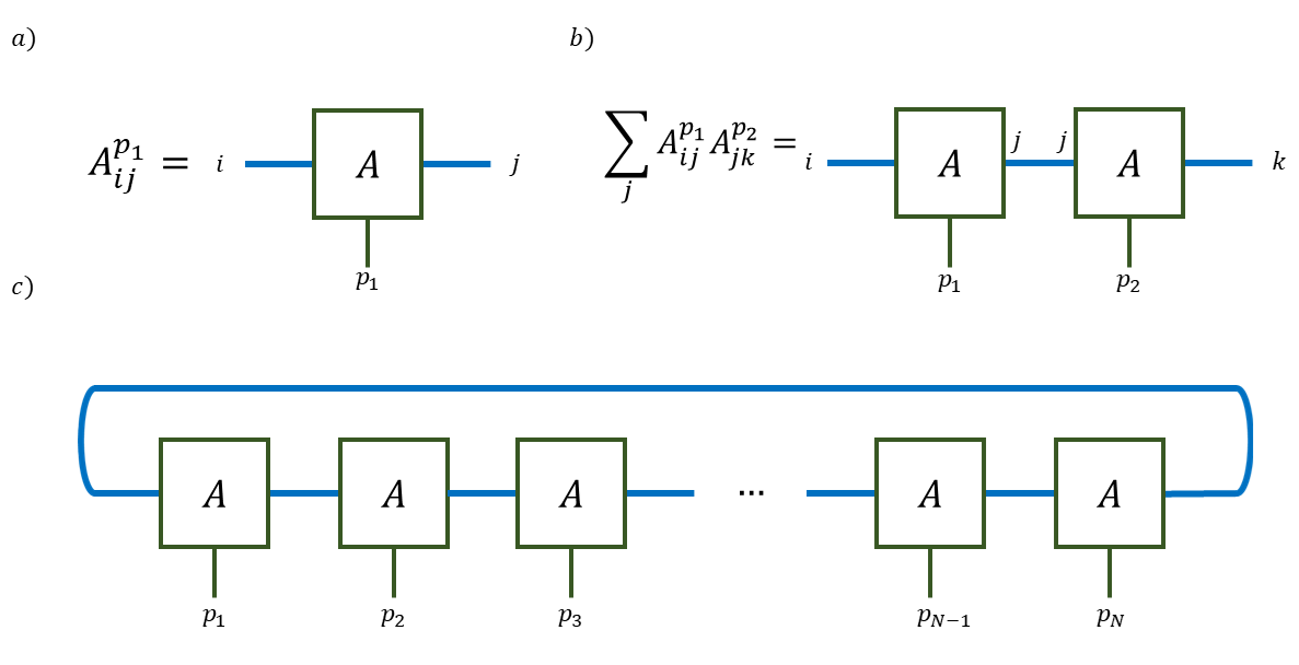
Figure 6: a) The graphical representation of a rank-three tensor A with the physical index $p_{1}$ and virtual indices $i,j$. b) Representation of the rank-four tensor $\sum_{j}A^{p_{1}}_{i,j}A^{p_{2}}_{j,k}$, with two physical and two virtual indices, just as Einstein’s convention, any connected legs are assumed to be summed over. c) MPS representation of a general translational invariant state with periodic boundary conditions.

In 1D, we can label the spatial positions of sites by $i$, and this Schmidt decomposition is then interpreted as the cutting of the chain into two left and right sub-chains. The von Neuman entanglement entropy between these two sub-chains is:

$$\mathrm{S}\left(\rho_{Left}\right) =\mathrm{S}\left(\rho_{Right}\right)=-\operatorname{Tr}\left[\rho_{Left}\log\rho_{Left}\right]$$

$$=\sum_{r}^{r_{max}}-\lambda_{r}^{2}\log(\lambda_{r}^{2})\leq\log{(r_{max})}$$ (11)

For local gapped Hamiltonians with a non-degenerate ground state, the area law of entropy was proven rigorously in 1D setting $\mathrm{S}$ to be less than a constant independent of the sub-chain length [44, 45]. Therefore, we only need an MPS with a finite dimension to capture the entanglement in the infinite system. MPS is then a cornerstone in studying 1D systems of gapped Hamiltonians and a lot of properties are clearer in this representation as we will discuss. It is often more convenient to use a graphical representation to express MPS operations where tensors are represented by a certain shape and the legs correspond to indices. Linking legs is a convention for summation see Fig. 6

A1 Injective MPS

There is large gauge freedom $A_{p_{1}}\to XA_{p_{1}}X^{-1}$ in the representation of any wavefunction using MPS. This gauge freedom can be exploited to put the matrices in the right-canonical form $\sum_{p_{i}}A^{p_{i}}A^{\dagger p_{i}}=\mathbb{I}$ to facilitate both computational and theoretical evaluations of the MPS. If we also define the transfer matrix $\mathbb{E}_{ii^{\prime},jj^{\prime}}=\sum_{p}A^{p}_{ij}A^{{\dagger}p}_{i^{\prime}j^{\prime}}$, then the right-canonical form means that $\mathbb{I}$ is a right fixed point for the transfer matrix Fig. 7. Injective MPS are a finer restriction after this initial gauge fixing. They intuitively represent finitely correlated ground states which have only short-ranged entanglement. They exclude the so-called cat states which are a superposition of macroscopically different states such as the GHZ state.

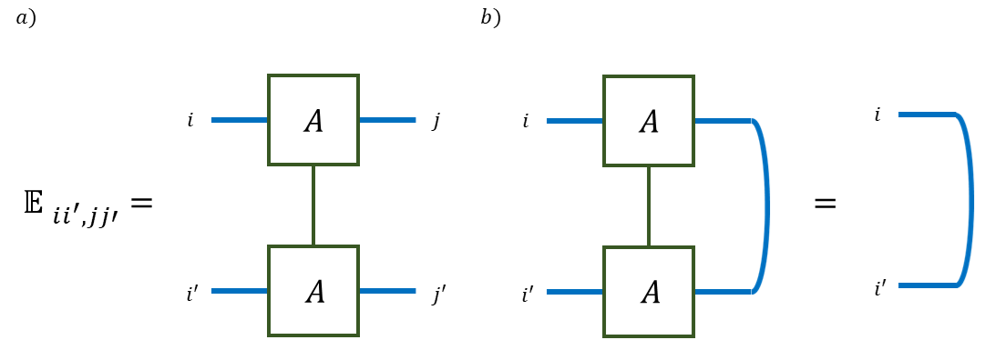
Figure 7: a) The graphical representation of the rank-four tensor $\mathbb{E}$ representing the transfer matrix with the implicit summation over the physical index $p$. The matrix A in the bottom row is understood to represent $A^{\dagger}_{i^{\prime}j^{\prime}}$. b) The right-canonical condition $\mathbb{E}_{ii^{\prime},jj^{\prime}}\delta_{jj^{\prime}}=\delta_{ii^{\prime}}$

The right-canonical form along with injectivity implies the following properties [36, 37]:

• There exists $n_{0}$ such that $A^{p_{1}}A^{p_{2}}\cdots A^{p_{n}}$ for $(n\geq n_{0})$ span the $D\times D$ matrices.

• $\sum_{p_{i}}A^{p_{i}}A^{p_{i}\dagger}=\mathbb{I}$ and for the dual map $\sum_{p_{i}}A^{p_{i}\dagger}\Lambda A^{p_{i}}=\Lambda$, where $\Lambda$ is a full-rank positive diagonal matrix with unit trace.

• $\mathbb{I}$ is the only right eigenvector with eigenvalue $|\lambda_{\mathbb{I}}|=1$ and all other eigenvalues have strictly smaller magnitudes.

The fact that $\mathbb{I}$ is the only right eigenvector with eigenvalue can be viewed as a normalization condition. As $\bra{\psi}\ket{\psi}$ amounts to multiplying $\Tr(\mathbb{E^{N}})$ where $N$ is the size of the system. For large $N$, $\mathbb{E}$ can be decomposed intuitively in terms of its dominant right and left eigenvectors $\innerproduct{\psi}{\psi}=\Tr(\mathbb{E}^{N})\approx\Tr([\ket{\mathbb{I}}\bra{\Lambda}]^{N})=\bra{\Lambda}\ket{\mathbb{I}}=1$. The second consequence is that the correlation length is bounded by the second-largest eigenvalue $\lambda_{2}$: $\xi=-\frac{1}{\log\left|\lambda_{2}\right|}$. This is consistent with the fact that they represent finitely correlated states.

Appendix B Detection of Haldane Phase

Since Haldane’s conjecture in 1983 [12], a lot of properties of the Haldane phase were understood gradually, first of all, the existence of the gap itself can be used to detect the phase when all other phases are gapless. After the AKLT model, we know that the edge states will have spin-$\frac{1}{2}$ which can also be used to detect the phase. A hidden $\mathbb{Z}_{2}\times\mathbb{Z}_{2}$ symmetry was shown to illustrate how symmetry breaking in one model can be related to the string order in another [46]. The string order was also developed as a way of detecting the long-range order while having no long-range entanglement [32]. The entanglement spectrum of the state while short-ranged was shown to have at least double degeneracy [47]. The string order parameter was later shown to work only in the specific case of an abelian symmetry with at least two generators [48]. The renormalization-group flow of the state is a powerful tool that can also be used to detect and classify non-trivial SPTs [49]. The Haldane phase in spin-1 chains in 1D belongs to the class of symmetry-protected topological phases; the ground state is only topological if a symmetry is imposed on the perturbations of the Hamiltonian. In the absence of symmetry, the ground state can be connected adiabatically to the trivial product state $\ket{0}\otimes\ket{0}\dots$ [23]. It was shown that the Haldane phase can be protected by spatial inversion centered along a bond, time reversal symmetry, or $\mathbb{Z}_{2}\times\mathbb{Z}_{2}$ internal symmetry [23]. Moreover, qualifying Haldane’s original conjecture, it will only be a non-trivial SPT phase in spin chains with odd integer spins [23].

B1 Haldane Phase in AKLT model

The AKLT model presented the first exactly solvable realization of the Haldane phase:

$$H_{\mathrm{AKLT}}=\sum_{i}\left[\frac{1}{2}\mathbf{S}_{i}\cdot\mathbf{S}_{i+1}+\frac{1}{6}\left(\mathbf{S}_{i}\cdot\mathbf{S}_{i+1}\right)^{2}+\frac{1}{3}\right]$$

In the AKLT model, the Hamiltonian is the projection of each two neighboring spin-1 particles into the spin-2 sector: $H=\sum_{i}P_{2}\left(\mathbf{S}_{i}+\mathbf{S}_{i+1}\right)$ Since the Hamiltonian is a projection, the ground state will have zero energy. The ground state can be formed by ensuring that any two neighboring spins have a total spin of 1 or 0. The method to ensure this is to write the physical spin-1 sites as a symmetric combination of two spin-$\frac{1}{2}$ virtual particles. These spin-$\frac{1}{2}$ particles are then taken to form a singlet bond between neighboring sites Fig. 8.

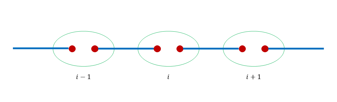
Figure 8: Schematic drawing of the ground state of the AKLT model. The red dots represent virtual spin-$\frac{1}{2}$ particles. The green circle designates a symmetrization of the two virtual spins on one site into a physical spin-1 in site $i$. The blue lines represent a singlet state of the two virtual spins on neighboring sites.

B2 MPS representation of AKLT Ground State

The ground state of the AKLT model has a nice description in terms of three $2\times 2$ matrices $A^{p}$ where $p$ stands for the spin index for standard basis $S^{z}=\{-1,0,1\}$ [36, 50].

$$A^{1}=\begin{pmatrix}0&0\\ -\frac{1}{\sqrt{2}}&0\end{pmatrix},\;A^{0}=\begin{pmatrix}\frac{1}{2}&0\\ 0&-\frac{1}{2}\end{pmatrix},\;A^{-1}=\begin{pmatrix}0&\frac{1}{\sqrt{2}}\\ 0&0\end{pmatrix}$$ (12)

Those matrices can be combined into a rank-three tensor $A^{p_{1}}_{ij}$ here $p_{1}$ represents the physical spin index $p_{1}\in\{-1,0,1\}$ and $i\text{,}j$ are virtual indices $i,j\in\{1,2\}$. It can be checked that these matrices represent the ground state for open or periodic boundary conditions respectively:

$$\ket{\Psi_{AKLT}}_{\text{OBC}} =\sum_{\alpha}\tilde{A}_{\alpha_{1}}^{p_{1}}A_{\alpha_{1}\alpha_{2}}^{p_{2}}\cdots\tilde{A}_{\alpha_{N}}^{p_{N}}\ket{p_{1}}\otimes\cdots\otimes\ket{p_{N}}$$ (13)

$$\ket{\Psi_{AKLT}}_{\text{PBC}} =\mathrm{Tr}(A^{p_{1}}A^{p_{2}}\cdots A^{p_{N}})\ket{p_{1}}\otimes\cdots\otimes\ket{p_{N}}$$ (14)

Here the summation is over all $\alpha_{i}$. In open boundary conditions: $\tilde{A}^{p_{1}}_{\alpha_{1}}$ is equivalent to ${A}_{\alpha_{0}\alpha_{1}}$ for $\alpha_{0}$ free index representing the unlinked virtual spin-$\frac{1}{2}$ at the left end of the open chain. Similarly, $\tilde{A}^{p_{N}}_{\alpha_{N}}$ is equivalent to ${A}_{\alpha_{N}\alpha_{N+1}}$ with $\alpha_{N+1}$ free index.

B3 Projective Representations

The projective representations of the Hamiltonian symmetries are the basis of the classification of SPT phases in 1D [20]. Injective MPS has the property that if there are two injective-MPS descriptions of the same state (up to a phase), then the matrices are related by a unitary up to a phase [51].

$$\{\ket{\Psi} =\mathrm{Tr}(A^{p_{1}}A^{p_{2}}\cdots A^{p_{N}})\ket{p_{1}}\otimes\ket{p_{2}}\dots\otimes\ket{p_{N}}$$

$$=e^{i\theta}\mathrm{Tr}(B^{p_{1}}B^{p_{2}}\cdots B^{p_{N}})\ket{p_{1}}\otimes\ket{p_{2}}\dots\otimes\ket{p_{N}}\}$$

$$\implies A^{p_{i}}=e^{i\phi}VB^{p_{i}}V^{{\dagger}}$$ (15)

In SPT phases, the states do not break any of the symmetries of the Hamiltonian. Therefore, the symmetry $g\subset G$ should at most change the matrices by a unitary $V_{g}$ and a phase $e^{i\phi{(u_{g})}}$. While the symmetry has a linear unitary representation on the physical states $u_{g}$, it has a projective representation on the virtual dimensions of the MPS matrices $V_{g}$ Fig. 9.

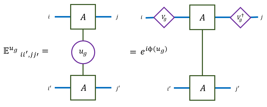
Figure 9: The first equality is the definition of the generalized transfer matrix $\mathbb{E}^{u_{g}}$, the second equality shows the correspondence of the linear representation $u_{g}$ on physical indices and the projective representation $V_{g}$ on virtual indices.

The different SPT phases respect the symmetries of the Hamiltonian but realize it in a projectively different way. This led to the classification of the SPT phase in translationally invariant 1D according to $H^{1}(G,U(1))\times H^{2}(G,U(1))$ where $H^{1}$ is the first cohomology group classifying different 1D representations of the group $G$ (this is the $e^{i\phi{(u_{g})}}$ part) and $H^{2}$ is the second cohomology group classifying the projective representation of the group $G$ (this is the $V_{g}$ part) [20]. Other symmetries like time-reversal symmetry require more careful treatment as it is anti-unitary but, the classification still follows the case presented here closely [48, 52].

B4 Hidden $\mathbb{Z}_{2}\times\mathbb{Z}_{2}$ Symmetry

One of the first insights on the Haldane phase came in 1992 when Kennedy and Tasaki showed that the model after a unitary non-local transformation on each site $j$: $U_{\mathrm{KT}}=\prod_{j<k}e^{i\pi S_{j}^{z}S_{k}^{x}}$ will result in a short-ranged Hamiltonian [46]:

$$H_{KT} =\sum_{j}S_{j}^{x}e^{i\pi S_{j+1}^{z}}S_{j+1}^{x}+S_{j}^{y}e^{i\pi S_{j}^{z}+S_{j+1}^{x}}S_{j+1}^{y}$$

$$+S_{j}^{z}e^{\left(i\pi S_{j}^{z}\right)}S_{j+1}^{z}$$ (16)

This transformation was generalized to higher spins by Oshikawa [53]. Both the old and new Hamiltonians are symmetric under the discrete global Dihedral group $D_{2}$ which is here the $\pi$-rotations about the three spin axes. This group is generated by rotations about the y and z axes: $e^{i\pi S_{x}}\text{ and }e^{i\pi S_{z}}$ (as the rotation around the y-axis is just their product). In the new Hamiltonian, the Haldane phase is mapped to a Ferromagnetic phase which spontaneously breaks the $\mathbb{Z}_{2}\times\mathbb{Z}_{2}$ Symmetry. The ferromagnetic phase is well understood under the Landau symmetry-breaking picture. The correlation function in the infinite limit $\lim_{|i-j|\to\infty}\langle S_{z}^{i}S_{z}^{j}\rangle$ will have a non-zero value for the ferromagnetic phase. Using the reverse transformation and noting $U_{\mathrm{KT}}U_{\mathrm{KT}}=\mathbb{I}$ we find that this correlation function in $H_{KT}$ is mapped to $\hat{O}_{\text{string}}=\lim_{|i-j|\to\infty}\langle S_{i}^{z}[\Pi_{k=i+1}^{j-1}e^{i\pi S_{k}^{z}}]S_{j}^{z}\rangle$ in the original Hamiltonian. This is just the string order parameter associated with the Haldane phase.

B5 String order Parameter

The string order parameter was first introduced by den Nijs [32]. It was motivated by the roughening phase transitions of crystals and related to the AKLT model. The configuration of the ground state of the AKLT model amounts to taking the superposition of all states satisfying simple rules: there is no restriction on the number or position of sites with spin $S^{z}=0$, no two consecutive sites with spin $S^{z}=1$ or $S^{z}=-1$ are allowed (even after excluding the zeroes). The ground state is formed by taking the superposition of all states satisfying this criterion. A representative term in the ground state is then: $\ket{1}\otimes\ket{0}\otimes\ket{0}\otimes\ket{-1}\otimes\ket{1}\otimes\ket{-1}\otimes\ket{1}\otimes\ket{-1}$ where $\ket{\pm 1}\coloneqq\ket{S^{z}=\pm 1}$. This is just the usual anti-ferromagnetic order as realized in the Neel state but with arbitrary zeroes in between. It is called diluted antiferromagnetic order. The string order parameter then captures the parity of spin flips and ignores the intermediate zeros. The string order can also be understood in the language of injective MPS.

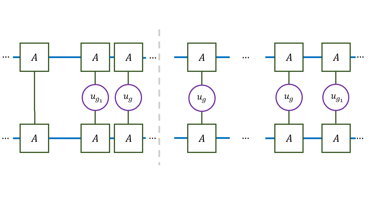
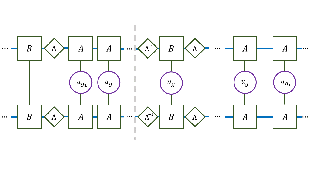
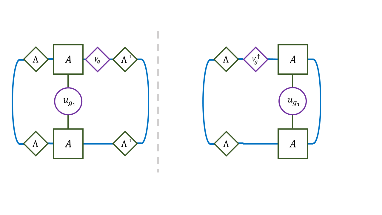
Figure 10: The general string order parameter $\hat{O}_{\text{general string}}=\lim_{N\to\infty}u(g_{1})_{1}[\Pi_{j=2}^{N-1}u(g)_{j}]u(g_{1})_{N}$ applied in the physical space. We can put the left and middle matrices in the left-canonical form. The two forms are related by $A^{p_{i}}=\Lambda^{-1}B^{p_{i}}\Lambda$. For a sufficiently long string, we can replace the left and right canonical matrices with identity. This string can also be seen as acting projectively with unitaries $V_{g}$ that will cancel except on the edges.

B6 General String Order Parameter

In general, if we have two symmetries that commute in the physical space $g,g_{2}\in G$ and $[u(g),u(g_{2})]=0$ where $G$ is the symmetry group of the Hamiltonian. However, projectively they obey $V_{g_{2}}V_{g}=e^{i\phi}V_{g}V_{g_{2}}$ We can find a third operator $g_{1}$ such that $u(g_{2})u(g_{1})=e^{i\sigma}u(g_{1})u(g_{2})$. Our general string operator will then be:

$$\hat{O}_{\text{general string}}=\lim_{N\to\infty}u(g_{1})_{1}[\Pi_{j=2}^{N-1}u(g)_{j}]u(g_{1})_{N}$$ (17)

In the bulk of the string, we can use injectivity to make $u_{g}$ act projectively on the virtual dimensions. These unitaries will cancel except on the two edges. If this string is long enough we can again use injectivity to effectively separate it into two terms. This will give $0$ if $\sigma\neq\phi$ in two symmetry-respecting phases. In Fig. 10 the string order parameter is broken down using the exchange of some right-canonical matrices to left-canonical matrices using $A^{p_{i}}=\Lambda^{-1}B^{p_{i}}\Lambda$ where this $\Lambda$ is the same matrix appearing in section  A1. If the string is long enough we can exploit the canonical form to reduce the left and right infinite chains to identity [54, 48]. We only pick up some $\Lambda$($\Lambda^{-1}$) due to the shift of the orthogonality center. It should be noted that $\Lambda$ will commute with any symmetry operator, as it represents the entanglement spectrum and this should remain invariant under the symmetry. This can also be seen from section  A1. If we define $L_{{g_{1}}}=\sum_{ii^{\prime}}{\Lambda^{2}_{ii^{\prime}}\mathbb{E}^{u_{g_{1}}}_{ii^{\prime},jj^{\prime}}}$ and $R_{{g_{1}}}=\sum_{j}{\mathbb{E}^{u_{g_{1}}}_{ii^{\prime},jj}}$ for the left and right transfer matrices taking into account the extra $\Lambda$, we arrive at:

$$\hat{O}_{\text{general string}}=\Tr(L_{g_{1}}V_{g}\Lambda^{-2})\Tr(V_{g}^{\dagger}R_{{g_{1}}}\Lambda^{2})$$ (18)

Since $u(g_{2})$ commutes with $u(g_{1})$ up to a phase $\sigma$ but projectively it commutes with $V_{g}$ up to another phase $\phi$. The left trace then obeys $\Tr(L_{g_{1}}V_{g}\Lambda^{-2})=e^{i(\sigma-\phi)}\Tr(L_{g_{1}}V_{g}\Lambda^{-2})$ and thus it will vanish for $\sigma\neq\phi$ as desired [48]. In Haldane phase, we have the two symmetries $g\to e^{i\pi S_{x}}$, $g_{2}\to e^{i\pi S_{z}}$ and $g_{1}\to S_{z}$. $\sigma$ is $\pi$ so $e^{i\pi S_{z}}$ and $e^{i\pi S_{x}}$ have to anti-commute virtually to give non-zero string order. The two $\pi$ rotations would commute for a spin-1 chain. However, owing to the topological nature of the phase the edges here are effectively spin-$\frac{1}{2}$ states whose rotation matrices form a representation of SU(2) and anti-commute.

References

- Kitaev [2001] A. Y. Kitaev, Unpaired majorana fermions in quantum wires, Physics-Uspekhi 44, 131–136 (2001).
- Sarma et al. [2015] S. D. Sarma, M. Freedman, and C. Nayak, Majorana zero modes and topological quantum computation, Npj Quantum Inf. 1 (2015).
- Jaworowski and Hawrylak [2019] B. Jaworowski and P. Hawrylak, Quantum bits with macroscopic topologically protected states in semiconductor devices, Appl. Sci. (Basel) 9, 474 (2019).
- Bandres et al. [2018] M. A. Bandres, S. Wittek, G. Harari, M. Parto, J. Ren, M. Segev, D. N. Christodoulides, and M. Khajavikhan, Topological insulator laser: Experiments, Science 359, eaar4005 (2018).
- He et al. [2019] M. He, H. Sun, and Q. L. He, Topological insulator: Spintronics and quantum computations, Front. Phys. 14 (2019).
- Landau and Lifshitz [1996] L. D. Landau and E. M. Lifshitz, Statistical Physics, 3rd ed. (Butterworth-Heinemann, Oxford, England, 1996).
- Klitzing et al. [1980] K. v. Klitzing, G. Dorda, and M. Pepper, New method for high-accuracy determination of the fine-structure constant based on quantized hall resistance, Phys. Rev. Lett. 45, 494 (1980).
- Laughlin [1983] R. B. Laughlin, Anomalous quantum hall effect: An incompressible quantum fluid with fractionally charged excitations, Phys. Rev. Lett. 50, 1395 (1983).
- Tsui et al. [1982] D. C. Tsui, H. L. Stormer, and A. C. Gossard, Two-dimensional magnetotransport in the extreme quantum limit, Phys. Rev. Lett. 48, 1559 (1982).
- Haldane [1988] F. D. M. Haldane, Model for a quantum hall effect without landau levels: Condensed-matter realization of the “parity anomaly”, Phys. Rev. Lett. 61, 2015 (1988).
- Haldane [1983a] F. D. M. Haldane, Nonlinear field theory of large-spin heisenberg antiferromagnets: Semiclassically quantized solitons of the one-dimensional easy-axis néel state, Phys. Rev. Lett. 50, 1153 (1983a).
- Haldane [1983b] F. D. M. Haldane, Continuum dynamics of the 1-D heisenberg antiferromagnet: Identification with the o(3) nonlinear sigma model, Phys. Lett. A 93, 464 (1983b).
- Kane and Mele [2005a] C. L. Kane and E. J. Mele, topological order and the quantum spin hall effect, Phys. Rev. Lett. 95, 146802 (2005a).
- Kane and Mele [2005b] C. L. Kane and E. J. Mele, Quantum spin hall effect in graphene, Phys. Rev. Lett. 95, 226801 (2005b).
- Levin and Wen [2005] M. A. Levin and X.-G. Wen, String-net condensation: A physical mechanism for topological phases, Phys. Rev. B 71, 045110 (2005).
- Kitaev [2003] A. Y. Kitaev, Fault-tolerant quantum computation by anyons, Ann. Phys. (N. Y.) 303, 2 (2003).
- Wen [2017] X.-G. Wen, Colloquium: Zoo of quantum-topological phases of matter, Rev. Mod. Phys. 89, 041004 (2017).
- Chen et al. [2010] X. Chen, Z.-C. Gu, and X.-G. Wen, Local unitary transformation, long-range quantum entanglement, wave function renormalization, and topological order, Phys. Rev. B 82, 155138 (2010).
- Mesaros and Ran [2013] A. Mesaros and Y. Ran, Classification of symmetry enriched topological phases with exactly solvable models, Phys. Rev. B 87, 155115 (2013).
- Chen et al. [2011] X. Chen, Z.-C. Gu, and X.-G. Wen, Classification of gapped symmetric phases in one-dimensional spin systems, Phys. Rev. B 83, 035107 (2011).
- Bethe [1931] H. Bethe, Zur theorie der metalle, Zeit. für Physik 71, 205 (1931).
- Affleck et al. [1987] I. Affleck, T. Kennedy, E. H. Lieb, and H. Tasaki, Rigorous results on valence-bond ground states in antiferromagnets, Phys. Rev. Lett. 59, 799 (1987).
- Pollmann et al. [2012] F. Pollmann, E. Berg, A. M. Turner, and M. Oshikawa, Symmetry protection of topological phases in one-dimensional quantum spin systems, Phys. Rev. B 85, 075125 (2012).
- Poddubny and Glazov [2019] A. N. Poddubny and M. M. Glazov, Topological spin phases of trapped rydberg excitons in , Phys. Rev. Lett. 123, 126801 (2019).
- Urban et al. [2009] E. Urban, T. A. Johnson, T. Henage, L. Isenhower, D. D. Yavuz, T. G. Walker, and M. Saffman, Observation of rydberg blockade between two atoms, Nat. Phys. 5, 110 (2009).
- Knox [1963] R. S. Knox, Theory of Excitons (Academic Press, San Diego, CA, 1963).
- Walther et al. [2018] V. Walther, S. O. Krüger, S. Scheel, and T. Pohl, Interactions between rydberg excitons in , Phys. Rev. B 98, 165201 (2018).
- Peyronel et al. [2012] T. Peyronel, O. Firstenberg, Q.-Y. Liang, S. Hofferberth, A. V. Gorshkov, T. Pohl, M. D. Lukin, and V. Vuletić, Quantum nonlinear optics with single photons enabled by strongly interacting atoms, Nature 488, 57 (2012).
- Bernien et al. [2017] H. Bernien, S. Schwartz, A. Keesling, H. Levine, A. Omran, H. Pichler, S. Choi, A. S. Zibrov, M. Endres, M. Greiner, V. Vuletić, and M. D. Lukin, Probing many-body dynamics on a 51-atom quantum simulator, Nature 551, 579 (2017).
- Bluvstein et al. [2023] D. Bluvstein, S. J. Evered, A. A. Geim, S. H. Li, H. Zhou, T. Manovitz, S. Ebadi, M. Cain, M. Kalinowski, D. Hangleiter, J. P. B. Ataides, N. Maskara, I. Cong, X. Gao, P. S. Rodriguez, T. Karolyshyn, G. Semeghini, M. J. Gullans, M. Greiner, V. Vuletić, and M. D. Lukin, Logical quantum processor based on reconfigurable atom arrays, Nature (2023).
- Taylor et al. [2022] J. Taylor, S. Goswami, V. Walther, M. Spanner, C. Simon, and K. Heshami, Simulation of many-body dynamics using rydberg excitons, Quantum Sci. Technol. 7, 035016 (2022).
- den Nijs and Rommelse [1989] M. den Nijs and K. Rommelse, Preroughening transitions in crystal surfaces and valence-bond phases in quantum spin chains, Phys. Rev. B 40, 4709 (1989).
- White [1992] S. R. White, Density matrix formulation for quantum renormalization groups, Phys. Rev. Lett. 69, 2863 (1992).
- Fishman et al. [2022] M. Fishman, S. R. White, and E. M. Stoudenmire, The ITensor Software Library for Tensor Network Calculations, SciPost Phys. Codebases , 4 (2022).
- Zauner-Stauber et al. [2018] V. Zauner-Stauber, L. Vanderstraeten, M. T. Fishman, F. Verstraete, and J. Haegeman, Variational optimization algorithms for uniform matrix product states, Phys. Rev. B 97, 045145 (2018).
- Fannes et al. [1992] M. Fannes, B. Nachtergaele, and R. F. Werner, Finitely correlated states on quantum spin chains, Commun. Math. Phys. 144, 443 (1992).
- Perez-Garcia et al. [2007] D. Perez-Garcia, F. Verstraete, M. M. Wolf, and J. I. Cirac, Matrix product state representations (2007), arXiv:quant-ph/0608197 [quant-ph] .
- Ejima et al. [2021] S. Ejima, F. Lange, and H. Fehske, Quantum criticality in dimerised anisotropic spin-1 chains, Eur. Phys. J. Spec. Top. 230, 1009 (2021).
- Tzeng et al. [2017] Y.-C. Tzeng, H. Onishi, T. Okubo, and Y.-J. Kao, Quantum phase transitions driven by rhombic-type single-ion anisotropy in the haldane chain, Phys. Rev. B 96, 060404 (2017).
- Ren et al. [2018] J. Ren, Y. Wang, and W.-L. You, Quantum phase transitions in spin-1 chains with rhombic single-ion anisotropy, Phys. Rev. A 97, 042318 (2018).
- Wu et al. [2023] H. Y. Wu, Y.-C. Tzeng, Z. Y. Xie, K. Ji, and J. F. Yu, Exploring quantum phase transitions by the cross derivative of the ground state energy, New J. Phys. 25, 043006 (2023).
- Poddubny and Glazov [2020] A. N. Poddubny and M. M. Glazov, Polarized edge state emission from topological spin phases of trapped rydberg excitons in , Phys. Rev. B 102, 125307 (2020).
- Vidal [2003] G. Vidal, Efficient classical simulation of slightly entangled quantum computations, Phys. Rev. Lett. 91, 147902 (2003).
- Hastings [2007] M. B. Hastings, An area law for one-dimensional quantum systems, J. Stat. Mech. 2007, P08024 (2007).
- Aharonov et al. [2011] D. Aharonov, I. Arad, U. Vazirani, and Z. Landau, The detectability lemma and its applications to quantum hamiltonian complexity, New J. Phys. 13, 113043 (2011).
- Kennedy and Tasaki [1992] T. Kennedy and H. Tasaki, Hidden × symmetry breaking in haldane-gap antiferromagnets, Phys. Rev. B 45, 304 (1992).
- Pollmann et al. [2010] F. Pollmann, A. M. Turner, E. Berg, and M. Oshikawa, Entanglement spectrum of a topological phase in one dimension, Phys. Rev. B 81, 064439 (2010).
- Pollmann and Turner [2012] F. Pollmann and A. M. Turner, Detection of symmetry-protected topological phases in one dimension, Phys. Rev. B 86, 125441 (2012).
- Gu and Wen [2009] Z.-C. Gu and X.-G. Wen, Tensor-entanglement-filtering renormalization approach and symmetry-protected topological order, Phys. Rev. B 80, 155131 (2009).
- Totsuka and Suzuki [1995] K. Totsuka and M. Suzuki, Matrix formalism for the VBS-type models and hidden order, J. Phys. Condens. Matter 7, 1639 (1995).
- Bridgeman and Chubb [2017] J. C. Bridgeman and C. T. Chubb, Hand-waving and interpretive dance: an introductory course on tensor networks, J. Phys. A Math. Theor. 50, 223001 (2017).
- Vancraeynest-De Cuiper et al. [2023] B. Vancraeynest-De Cuiper, J. C. Bridgeman, N. Dewolf, J. Haegeman, and F. Verstraete, One-dimensional symmetric phases protected by frieze symmetries, Phys. Rev. B 107, 115123 (2023).
- Oshikawa [1992] M. Oshikawa, Hidden Z2*Z2symmetry in quantum spin chains with arbitrary integer spin, J. Phys. Condens. Matter 4, 7469 (1992).
- Pérez-García et al. [2008] D. Pérez-García, M. M. Wolf, M. Sanz, F. Verstraete, and J. I. Cirac, String order and symmetries in quantum spin lattices, Phys. Rev. Lett. 100, 167202 (2008).