Emergence of Hidden Capabilities:
Exploring Learning Dynamics in Concept Space

Abstract

Modern generative models demonstrate impressive capabilities, likely stemming from an ability to identify and manipulate abstract concepts underlying their training data. However, fundamental questions remain: what determines the concepts a model learns, the order in which it learns them, and its ability to manipulate those concepts? To address these questions, we propose analyzing a model’s learning dynamics via a framework we call the concept space, where each axis represents an independent concept underlying the data generating process. By characterizing learning dynamics in this space, we identify how the speed at which a concept is learned, and hence the order of concept learning, is controlled by properties of the data we term concept signal. Further, we observe moments of sudden turns in the direction of a model’s learning dynamics in concept space. Surprisingly, these points precisely correspond to the emergence of hidden capabilities, i.e., where latent interventions show the model possesses the capability to manipulate a concept, but these capabilities cannot yet be elicited via naive input prompting. While our results focus on synthetically defined toy datasets, we hypothesize a general claim on emergence of hidden capabilities may hold: generative models possess latent capabilities that emerge suddenly and consistently during training, though a model might not exhibit these capabilities under naive input prompting.

1 Introduction

Modern generative models, such as text-conditioned diffusion models, show unprecedented capabilities [1, 2, 3, 4, 5, 6, 7, 8]. These abilities have led to use of such models in applications as valuable as training control policies for robotics [9, 10, 11] and models for weather forecasting [12], to as drastic as campaigning in democratic elections [13, 14]. Similar claims can be made for generative models of other modalities, e.g., large language models (LLMs) [15, 16, 17, 18], speech and audio models [19, 14], or even systems designed for enabling scientific applications such as drug discovery [20, 21]. Arguably, acquiring such general capabilities requires for models to internalize the data-generating process and disentangle the concepts (aka latent variables or factors of variation) underlying it [22, 23]. Flexibly manipulating these concepts can then enable generation of novel samples that are entirely out-of-distribution (OOD) with respect to the ones used for training [24, 25, 26, 27, 28].

As shown in prior work, modern generative models do exhibit signs of disentangling concepts underlying the data generating process and learning of corresponding capabilities to manipulate said concepts [29, 30, 31, 32, 33, 34, 35, 36, 37]. At the same time, contemporary work has argued that models’ capabilities can be unreliable, arbitrarily failing for a given input and succeeding on another [38, 39, 40, 41, 42, 43, 44]. Thus, critical questions remain on how generative models acquire their capabilities (see Fig. 1): what determines whether the model will disentangle a concept and learn the capability to manipulate it; are all concepts and corresponding capabilities learned at the same time; and is there a structure to the order of concept learning such that, given insufficient time, the model learns capabilities to manipulate only a subset of concepts but not others?

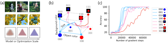
Figure 1: Concept Learning Geometry underlies emergence. (a) Top: A multimodal model learns to generate the concepts in the order of “astronaut”, “horse”, and finally “riding” as it scales up (adapted from Yu et al.[45]). Middle: “blue square apple” is generated in the order of “apple”, “square”, and “blue” (adapted from Li et al.[46]). Bottom: Despite its simplicity, our model trained on synthetic data shows concept learning dynamics where it first learns “shape” and then “color”. (b) Concept space is an abstract coordinate space where individual axes correspond to different concepts and a given point corresponds to a “concept class”, i.e., a predefined collection of concepts (e.g., large blue circles on bottom left corner). Traversal along axes of the concept space yield change in a specific property of the sample (e.g., going from large blue circle to large red circle along object color axis). Trajectories show a model’s dynamics in concept space for learning to generate classes shown in-distribution (blue nodes) versus out of distribution (pink nodes). As we show, dynamics in concept space are highly interpretable, enabling precise comments on which concepts the model learns first, why, and what order it follows. (c) Measuring how accurately a model generates samples from a given concept class, showing an order of concept learning: first background color is learned, then size, and then object color.

This work. To address the questions above, we propose to analyze a model’s learning dynamics at the granularity of concepts. Since performing such an analysis on realistic, off-the-shelf datasets can be challenging, we develop synthetic toy datasets of 2D objects with different concepts (e.g., shape, size, color) that give us thorough control over the data-generating process and allow for an exhaustive characterization of the model’s learning dynamics (see Fig. 1). Our contributions are as follows.

• Introducing Concept Space. We propose to evaluate a model’s learning dynamics in the concept space—an abstract coordinate system whose axes correspond to specific concepts underlying the data-generating process. We instantiate a notion of underspecification in concept space and establish its effects on a model’s (in)ability to disentangle concepts.

• Concept Signal Dictates Speed of Learning. We find the speed at which a model disentangles a concept and learns the capability to manipulate it is dictated by the sensitivity of the data-generating process to changes in values of said concept—a quantity we call concept signal. We show concept signals shape the geometry of a learning trajectory and hence control the overall order of concept learning.

• Sudden Transitions in Concept Learning. We use analytical curves to explain the phenomenology of learning dynamics in concept space, showing the dynamics can be divided into two broad phases: (P1) learning of a hidden capability, whereby even if the model does not produce the desired output for a given input, there exist systematic latent interventions that lead the model to generate the desired output, and (P2) learning to generate the desired output from the input space.

Overall, while our results focus on a toy synthetic task and text-to-image diffusion models, we hypothesize a broader claim on hidden emergence of latent capabilities holds true: generative models possess latent capabilities that are learned suddenly and consistently during training, but these capabilities are not immediately apparent since prompting the model via the input space may not elicit them, hence hiding how “competent” the model actually is [47, 48]. Empirically, signs of “hidden capabilities” have already been shown in generative models at scale [49, 50, 51, 52, 53, 45], and our results help provide a formal framework to partially ground such results.

2 Related Work

Concept learning. The term concepts as used in this work is broadly equivalent to the notion of factors of variation from prior work on disentangled representation learning [23, 54, 55, 56, 57, 30, 58, 59, 60], and is motivated by use of the term in a similar sense in cognitive science [61, 62, 63, 64, 65, 66]. The focus of literature on disentanglement has been to prove identifiability results, e.g., when will a generative model trained on a dataset learn to invert the data-generating process, hence identifying the latent variables, i.e., concepts, that underlie it. Given the success of modern generative models, we argue, despite impossibility results from prior work, these models are in fact learning to disentangle some, if not all, concepts. Precisely what guides which concepts are disentangled however requires studying the learning dynamics—the target of our work.

Interpretability. A growing line of papers demonstrate highly interpretable representations of intuitive concepts exist in generative models, especially LLMs [67, 68, 69, 70, 71, 72]. Similar work in this vein in image diffusion models has found semantic representations in various components of the model [52, 73, 74, 75, 37]: e.g., existence of linear representations for concepts such as 3D depth or object versus background distinctions [76, 77] . These papers further bolster our argument, modern generative models are truly inverting the data-generating process and identifying the concepts underlying it.

Competence vs. performance. In cognitive science, a system’s competence on a task is often contrasted with its performance [48, 47, 78, 79, 80, 81]: competence is the system’s possession of a capability (e.g., to converse in a language) and performance is system’s use of that capability in concrete situations [78]. For example, a bilingual person may generally converse in their primary language $\mathcal{L}$, despite possessing knowledge of another language $\mathcal{L}^{\prime}$, unless it is crucial to use the latter—clearly, they are competent in both languages, but gauging their performance on $\mathcal{L}^{\prime}$ requires appropriately “prompting” them to use it. One can analogize this distinction with remarks on a neural network possessing a capability versus us being able to elicit it on predefined benchmarks and measure their performance [82, 83, 84, 85]. For example, on the BigBench benchmark [86], LLMs were shown to have perform poorly on several tasks, but follow up work [87] showed mere chain-of-thought prompting [49, 50] leads to huge boosts on all tasks. This indicates the evaluated models were in fact “competent”, but inappropriate prompting led to undermining how “performant” they are.

3 Concept Space: A Framework for Analyzing Concept Learning Dynamics

We first formally introduce our framework of concept spaces. Motivated by a rich body of literature on disentangled representation learning [23, 54, 55, 56, 57, 30, 58, 59, 60], this framework allows us to systematically analyze how different concepts underlying the data generating process and corresponding capabilities to manipulate them are learned during training. We highlight that since our primary empirical focus in this paper will be an abstraction of text-to-image generative models, parts of the framework will be specifically instantiated with text-to-image generation tasks in mind. To this end, we note our model class of interest is a generative model $F$ that is trained using conditioning information $h$ to produce images $y$. For example, $F$ may be instantiated using a diffusion model that uses embeddings $h$ of textual descriptions of a scene to produce images $y$. We next define a concept space.

Definition 1.

(Concept Space.) Consider an invertible data-generating process $\mathcal{G}:\mathcal{Z}\to\mathcal{X}$ that samples vectors ${z}\sim P(\mathcal{Z})$ from a vector space $\mathcal{Z}\subset\mathbb{R}^{d}$ and maps them to the observation space $\mathcal{X}\in\mathbb{R}^{n}$. We assume the sampling prior is factorizable, i.e., $P({z}\in\mathcal{Z})=\Pi_{i=1}^{d}P({z_{i}})$, and individual dimensions of $\mathcal{Z}$ correspond to semantically meaningful concepts. Then, a concept space $\mathcal{S}$ is defined as the multidimensional space composed of all possible concept vectors $z$, i.e., $\mathcal{S}\coloneqq\{z\mid z\sim P(\mathcal{Z})\}$

As an example, consider a concept space defined using three concepts, say, ${z_{1}}=\text{{shape}}$, ${z_{2}}=\text{{size}}$, and ${z_{3}}=\text{{color}}$ that maps to a dataset of images with objects of different combinations of shapes, sizes, and colors (see Fig. 2). The assumption that concepts are independently distributed implies one can intervene on a given concept without affecting the other ones. For example, given a sample from the dataset above, the concept color in an image can be altered by changing the value of the relevant latent variable and mapping it to the image space via the data-generating process. Now, using a mixing function $\mathcal{M}$ that yields conditioning information $h\coloneqq\mathcal{M}(z)$, we can train a conditional generative model and define a notion of capabilities relevant to our work as follows.

Definition 2.

(Capability.) A concept class $\mathcal{C}$ denotes the set of concept vectors $z_{\mathcal{C}}$ such that a subset of dimensions of these vectors are fixed to predefined values. Classes $\mathcal{C}$ and $\mathcal{C}^{\prime}$ are said to differ in the $k^{\text{th}}$ concept if $\forall z\in z_{\mathcal{C}}$, there exists $z^{\prime}\in z_{\mathcal{C}^{\prime}}$ with $z[k]\neq z^{\prime}[k]$ and $z[i]=z^{\prime}[i]$ for $i\neq k$. We say a model possesses the “capability to alter the $k^{\text{th}}$ concept” if for any class $\mathcal{C}$ whose samples were seen during training, the model can produce samples from class $\mathcal{C}^{\prime}$ that differs from $\mathcal{C}$ in the $k^{\text{th}}$ concept.

Intuitively, the definition above comments on whether the model can flexibly manipulate concepts of classes seen during training to produce samples from classes that were not seen, i.e., classes that are entirely out-of-distribution. As an example, consider a concept space with shape, color, and size as concepts. If shape and color are fixed to circle and blue respectively, we get the class of blue circles; i.e., $\forall z\in z_{\text{{blue circles}}}$, the first and second dimension respectively take on values that correspond to the shape circle and color blue. Then, given a conditional diffusion model that was shown blue circles during training, we will say this model possesses the capability to alter the concept color if it can produce samples from concept classes with the same shape as circles, but different colors (e.g., red or green circles). Analyzing learning dynamics in the concept space will thus provide a direct lens into the model’s capabilities as they are acquired.

We also note that the definition above is not dependent on the precise manner via which the model is prompted to elicit an output, i.e., it need not be the case that the conditioning information $h$ that is used for training the model is used to evaluate the model capability. In fact, in our experiments, we will try alternative protocols such as intervening on the latent representations to show that substantially before the model can be prompted using $h$ to generate samples from an OOD concept class, it can generate samples from said class via such latent interventions. To this end, we also define a measure that assesses how much learning signal the data provides towards disentanglement of a concept, and hence learning of a capability to manipulate it.

Definition 3.

(Concept Signal.) The concept signal $\sigma_{i}$ for a concept $z_{i}$ measures the sensitivity of the data-generating process to change in the value of a concept variable, i.e., $\sigma_{i}\coloneqq\left|\nicefrac{{\partial\mathcal{G}(z)}}{{\partial z_{i}}}\right|$.

Intuitively, if the training objective is factorized at the granularity of concepts, concept signal indicates how much the model would benefit from learning about a concept. For example, consider a diffusion model trained using the MSE loss with conditioning $h\coloneqq z$ to predict the noise added to an image $\mathcal{G}(z)$. $\sigma_{i}$ is then merely the component of the loss representing how much change in conditioning $h$ yields changes in concept $z_{i}$, as it is represented in the image. Concept signal will thus serve as a crucial knob in our experiments to analyze learning dynamics in concept space and the order in which concepts are learned.

3.1 Experimental and Evaluation Setup

Figure 2: Concept spaces with different concept values see different concept signal. Consider a concept space comprised of concepts size and color. (Left) The color separation between the classes is stronger than the size separation, resulting in a stronger concept signal in the color dimension. (right) The size separation between the classes is stronger, thus resulting in a stronger signal for size.

Before proceeding further, we discuss our experimental setup that concretely instantiates the formalization above. Our data-generating process is motivated by prior work on disentanglement [54, 55, 56, 57, 58, 59, 60] and involves concept classes defined by three concepts, each with two values: color = $\{\text{red},\text{blue}\}$, size = $\{\text{large},\text{small}\}$, and shape=$\{\text{circle},\text{triangle}\}$. In Sec. 4.1 and Sec. 4.4, we use two attributes: color (with red labeled as 0 and blue as 1) and size (large labeled as 0 and small as 1). We generate a total of 2048 images for each class, with objects randomly positioned within each image. We train models on classes 00 (large red circles), 01 (large blue circles), and 10 (small red circles), shown as blue nodes in Fig. 2, and test using class 11 (small blue circles), shown as pink nodes, to evaluate a model’s ability to manipulate concepts and generalize OOD (see App. A.1 for further details). In Sec. 5, we will restrict to two attributes, shape=$\{\text{circle},\text{triangle}\}$ and color = $\{\text{red},\text{blue}\}$, and study the effect of noisy conditioning, i.e., what happens when concepts are correlated in the conditioning information $h$ due to some non-linear mixing function. For all experiments, we use a variational diffusion model [88] to generate $3\times 32\times 32$ images conditioned on vectors $h$ (see App. A.2 for further training details).

Evaluation Metric.

To assess whether a generated image matches the desired concept class without human intervention, we follow literature on disentangled representation learning [89, 54, 90, 91, 92, 55, 23, 30] and train classifier probes for individual concepts using the diffusion model’s training data. The probe architecture involves a U-Net [93] followed by an average pooling layer and $n$ MLP classification heads for the $n$ concept variables. See App. A.2 for further details.

4 Learning Dynamics in Concept Space

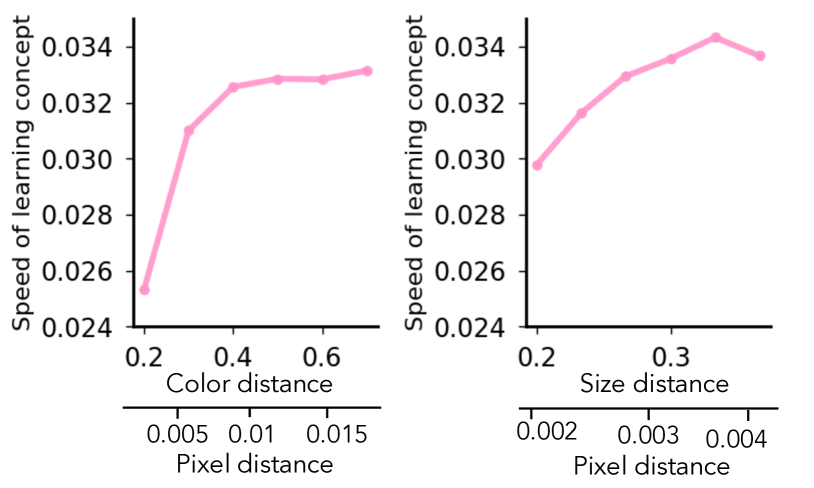
Figure 3: Concept signal determines learning speed. The speed of concept learning as an inverse of the time in gradient steps when the separation in color (left) and size (right) between different classes increases. Concept learning is faster when pixel differences among concept class and hence concepts are larger.

4.1 Concept Signal Determines Learning Speed

We first demonstrate the utility of concept signal as a tool to gauge at what rate the model learns a concept and the capability to manipulate it. To this end, we develop controlled variants of our data-generating process by changing the level of concept signal of each concept and train diffusion models conditioned with the latent concept vector $z$ on them. We primarily focus on concepts color and size, altering their concept signal by respectively adjusting the RGB contrast between red and blue and the size difference between large and small objects (see App. A.1 for details). We define the speed of learning each concept as inverse of the number of gradient steps required to reach 80% accuracy for class 11, i.e., the OOD class that requires learning the capability to manipulate concepts as seen during training. Results comparing different concept signals are shown in Fig. 3. For both color and size, we observe that concept signal dictates the speed at which individual concepts are learned. We also find that when different concepts have varying strengths of concept signals, this leads to differences in the learning speed for each concept.

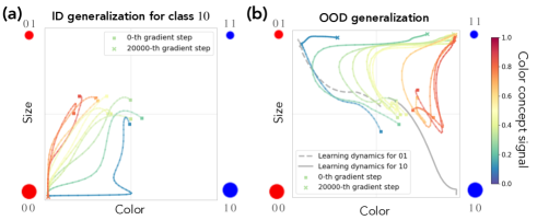
Figure 4: Concept signal governs generalization dynamics. (a) Learning dynamics in the concept space for in-distribution concept class 00 (bottom left). (b) Learning dynamics for out-of-distribution (OOD) concept class 11 (top right). We plot the accuracy for color on the x-axis and size on the y-axis. The [0,1) normalized color concept signal level is color coded. Two trajectories for 01 and 10 are shown to illustrate concept memorization.

4.2 Concept Signal Governs Generalization Dynamics

We next examine the model’s learning dynamics in concept space under various levels of concept signal for the concepts color and size. For completeness, we evaluate a model’s ability to generalize both in-distribution (ID) and OOD, but only the latter is deemed learning of a capability to manipulate a concept. Results are shown in Fig. 4, with panel (a) showing dynamics for learning to generate samples from ID class 00 and panel (b) showing dynamics for OOD class 11. Results on OOD generalization show a form of concept memorization, which we define as the phenomenon where the model’s generations on an OOD conditioning $h$ are biased towards the training class that helps define the strongest concept signal. For example, for the unseen conditioning 11, the generations are more alike 01 when the concept signal is stronger for size (e.g., blue curve in Fig. 4(b)) and alike 10 when the signal is stronger for color (e.g., red curve). Interestingly, we observe that for settings with high imbalance in concept signals, e.g., the blue curve in Fig. 4 (b), the endpoint of concept memorization is very biased towards one training class, here 01, delaying its out-of-distribution (OOD) generalization. For the learning trajectories of all classes, see Fig. 13 in App. C.2.

Broadly, our results imply that an early stopped text-to-image model can witness concept memorization and hence simply associate an unseen conditioning to the nearest concept class when asked to generate OOD samples (see Kang et al. [94] for a similar result in LLMs). However, given sufficient time, the model will disentangle concepts underlying the data-generating process and learn to generate entirely novel, OOD samples. For futher evidence in this vein, we also confirm our results across more general scenarios, including with the real-world CelebA dataset (App. C.3) and using three concept variables: color, background color, and size (App. C.4).

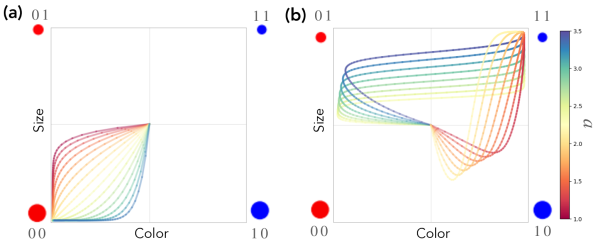
Figure 5: A Phenomenological Model of Learning Dynamics in Concept Space. Using Eq. 1, we simulate the learning trajectory for concept class 00 in panel (a) and the OOD class 11 in panel (b). Initially, target values are set at $(0,1)$ or $(1,0)$ based on the concept signal strengths for color or size, respectively. As the model progressively learns each concept, the target values gradually shift towards $(1,1)$. This simple toy model accurately reproduces the observed curves in Fig. 3(c), which arise from concept memorization.

4.3 Towards a Landscape Theory of Learning Dynamics

Fig. 4 indicates models undergo phases of understanding of concepts at different stages of training. In fact, an intriguing property of trajectories shown in Fig. 4 (b) is that there is a sudden turn in the learning dynamics from concept memorization to OOD generalization (e.g., see the top-left quadrant in Fig. 4 (b)). To investigate this further, we propose a minimal toy model that captures the geometry of model’s learning trajectories shown in that figure. Specifically, we use the following dynamics equation, $d(t)\coloneqq\tilde{z}+(\hat{z}-\tilde{z})\cdot\frac{1}{1+e^{-(t-\hat{t})}}$, where $\hat{z}$ is the target point we want to get to and $\tilde{z}$ is the initial, “biased” target. For example, consider the case with color and size concepts in Fig. 4 (b). The model’s generated samples are more alike class 01 and biased towards $(\tilde{z}_{1},\tilde{z}_{2})=(0,1)$ when the size concept signal $\sigma_{2}$ is stronger than $\sigma_{1}$; and to 10, $(\tilde{z}_{1},\tilde{z}_{2})=(1,0)$ when the color concept signal $\sigma_{1}$ is stronger than $\sigma_{2}$. We define $(\hat{z}_{1},\hat{z}_{2})$ as the target values or directions we want the learning to head towards (e.g., $(1,1)$ for OOD generalization). Based on this framework, we can derive the following energy function.

$$\frac{d{\bf z}}{dt}=-\nabla_{\bf z}L,\,\,L(z_{1},z_{2})=\begin{cases}\frac{1}{2a}\left(d(t-\hat{t}_{1})-z_{1}\right)^{2}+\frac{a}{2}(1-z_{2})^{2}&\text{if }\sigma_{1}>\sigma_{2},\\ \frac{1}{2a}(1-z_{1})^{2}+\frac{a}{2}\left(d(t-\hat{t}_{2})-z_{2}\right)^{2}&\text{otherwise}.\end{cases}$$ (1)

Here, $a$ is determined by the difference $|\sigma_{1}-\sigma_{2}|$ and $\hat{t}_{1}$ and $\hat{t}_{2}$ denote the times when the model learns concepts $z_{1}$ and $z_{2}$, respectively. Fig. 5 illustrates the simulated trajectories for classes 00 and 11, based on Eq. 1. Panels (a) and (b) correspond to classes 00 and 11, respectively. We define the actual target points $(\hat{z}_{1},\hat{z}_{2})$ as $(0,0)$ for class 00 and $(1,1)$ for class 11. For the initial targets $(\tilde{z}_{1},\tilde{z}_{2})$, we set both values to $(0,0)$ for class 00. For class 11, the targets are set to $(1,0)$ when $\sigma_{1}>\sigma_{2}$ and to $(0,1)$ when $\sigma_{1}<\sigma_{2}$. We find our toy model effectively captures the actual learning dynamics for both in-distribution (Fig. 3(b)) and out-of-distribution (OOD) concept classes (Fig. 3(c)). Notably, our simulation accurately replicates the two types of curves: clockwise (blue trajectory in Fig. 3(b)) and counterclockwise (red trajectory).

An important conclusion that follows from the results above is that the network’s learning dynamics can be precisely decomposed into two stages, hence yielding the sudden turns seen in trajectories in Fig. 4. We hypothesize there is a phase change underlying this decomposition and the model acquires the capability to alter concepts at this point of phase change. We investigate this next.

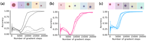
Figure 6: Emergence of hidden capabilities. We plot accuracy as a function of gradient steps for five different runs, using three different protocols for prompting the model to generate outputs for OOD concept classes. (a) The baseline, naive prompting protocol; (b) linear latent intervention, applied in the activation space; and (c) overprompting, akin to an intervention on the input space.

4.4 Sudden Transitions in Concept Learning Dynamics

The concept space visualization of learning dynamics observed in Fig. 4 (b) and our toy models analysis in Fig. 5 indicate that there exists a phase in which the model departs from concept memorization and disentangles each of the concepts, but still produces incorrect images. We claim that at the point of departure, the model has in fact already disentangled concepts underlying the data-generating process and acquired the relevant capabilities to manipulate them, hence yielding a change of direction in its learning trajectory. However, naive input prompting is insufficient to elicit these capabilities and generate samples from OOD classes, giving the impression the model is not yet “competent”. This then leads to the second phase in the learning dynamics, wherein an alignment between the input space and underlying concept representations is learned. We take the model corresponding to the second from left curve (the green curve) in Fig. 4 (b) to investigate this claim in detail. Specifically, given intermittent checkpoints along the model’s learning trajectory, we use the following two protocols for prompting the model to produce images corresponding to the class 11 (blue, small). See App. B for further details.

1. Activation Space: Linear Latent Intervention. Given conditioning vectors $h$, during inference we add or subtract components that correspond to specific concepts (e.g., $h_{\texttt{blue}}$).

2. Input Space: Overprompting. We simply enhance the color conditioning to values of higher magnitude, e.g. (0.4, 0.4, 0.6) to (0.3, 0.3, 0.7).

Fig. 6 shows the accuracy for five independent runs under: (a) naive input prompting, (b) linear latent interventions, and (c) overprompting. In Fig. 6 (a), we observe that some runs can produce samples from the target concept class (blue, small) with $\sim 100\%$ accuracy after around 8,000 gradient steps, while other runs fail to do so. However, in Fig. 6 (b, c), we find alternative protocols for prompting the model can consistently elicit the desired outputs much earlier than input prompting, e.g., at around as early as 6,000 gradient steps. This indicates the model does possess the capability to alter concepts and generalize OOD! Furthermore, we note that different protocols enable elicitation of the capability at approximately the same number of gradient steps, irrespective of the seed, and that this is precisely the point of sudden turn in the learning dynamics in Fig. 4! Interestingly, experiments with Classifier Free Guidance (CFG) [95] show that CFG only becomes effective after this transition (Fig. 16).

We further explore the second phase of learning in Appendix C.6 by patching the embedding module used for processing the conditioning information from the final checkpoint to an intermediate one. Our results show that when the final checkpoint does enable use of naive input prompting for eliciting a capability, the embedding module can be patched to an intermediate checkpoint and we can retrieve the desired output at approximately the same time that alternative prompting protocols start to work well. This suggests the second phase of learning primarily involves aligning the input space to intermediate representations that enable eliciting the model capabilities. Overall, our results above yield the following hypothesis.

Hypothesis 1. (Emergence of Hidden Capabilities.) Generative models possess hidden capabilities that are learned suddenly and consistently during training, but naive input prompting may not elicit these capabilities, hence hiding how “competent” the model actually is.

5 Effect of Underspecification on Learning Dynamics in Concept Space

In the results above, we use conditioning information that perfectly specifies concepts underlying the data-generating process, i.e., $h=z$. In practice, however, instructions are underspecified and one can thus expect correlations between concepts in the conditioning information extracted from those instructions [96, 97, 98, 99, 100]. For example, images of a strawberry are often correlated with the color red (see Fig. 7(a)). Correspondingly, unless a text-to-image model is shown explicit data stating “red strawberry” or images of non-red strawberries, the model’s ability to disentangle the concept color from the concept strawberry may be impeded (see generations for “yellow strawberry” in Fig. 7). Motivated by this, we next investigate the effects of using underspecified conditioning information on a model’s ability to learn concepts and capabilities to manipulate them.

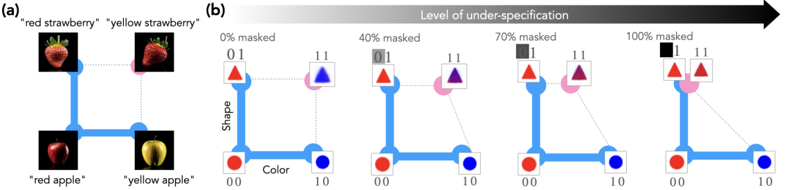
Figure 7: Underspecification and Concept Learning. (a) The state-of-the-art generative models [101] erroneously produces a red strawberry (top right corner) for the prompt “yellow strawberry”. (b) Without underspecification in the training data, a model $F$ accurately learns the concepts of shape and color, successfully generalizes to the unseen node blue triangle (leftmost). As masks are applied to the word red for the prompt red triangle, concept signal for triangle increasingly starts to correlate with the concept red. This causes the output images to change from blue to purple as the level of masking increases (panels left to right). Eventually, the color dimension for triangle collapses, biasing the model towards generating solely red triangles (rightmost).

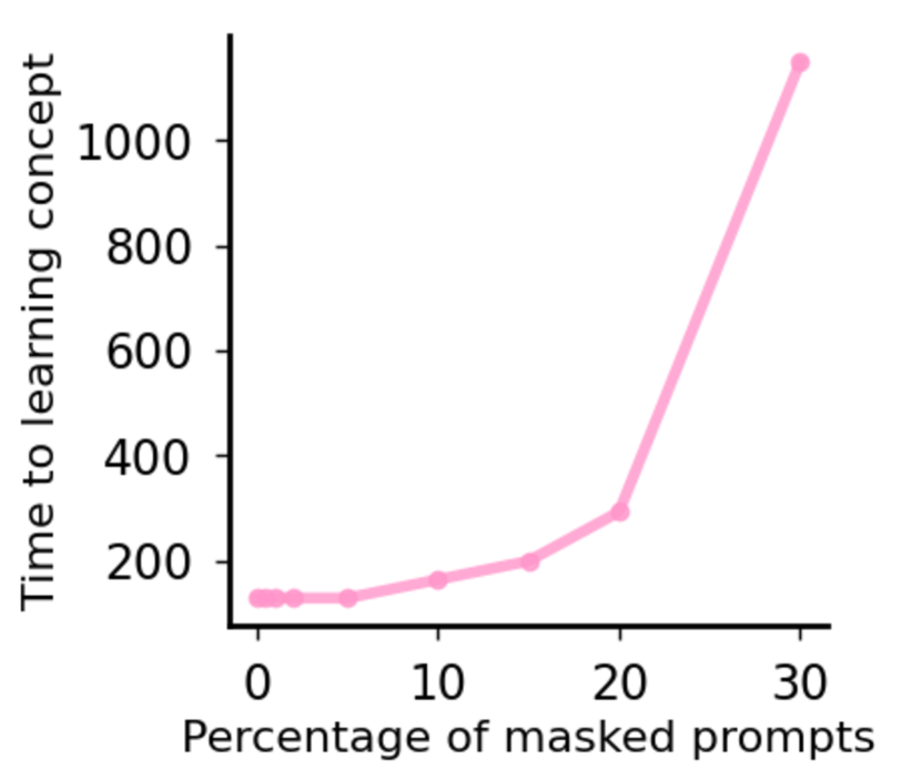
Figure 8: Underspecification delays out-of-distribution (OOD) generalization. The number of gradient steps required to reach accuracy above 0.8, as the percentage of masked prompts increases. A higher proportion of masked prompts slows down the speed of concept learning.

Experimental setup. The data generation and evaluation process follows the protocol described in Sec. 3.1. We select color (red and blue) and shape (circle and triangle) as the concepts, drawing an analogy to the “yellow strawberry” example. To simulate underspecification, we randomly select training samples that have a specific combination of shape and color (e.g., “red triangle”). We then mask the token representing the color (“red”) and train the model on three concept classes {00, 01, 10}, represented by blue nodes in Fig. 7, with some prompts masked. We test using class 11 (pink node) with no prompts masked, to see if the model has learned disentangled concepts and can generalize OOD.

Underspecification Delays and Hinders OOD generalization. Fig. 8 shows how underspecification (masked prompts) affects the speed of concept learning. We see that as the percentage of masked prompts increases, the speed of learning a concept decreases, suggesting that underspecification leads to slower learning of concepts. Further, Fig. 9 (a) shows models’ learning dynamics in concept space at varying levels of underspecification. With 0% masking, the model accurately produces an image of blue triangle (see Fig. 7(b)). However, as the percentage of masking increases, the color of generated images shifts from blue to purple (middle), and finally red. This demonstrates that when prompts are masked, the model’s understanding of shape triangle becomes intertwined with color red; even when blue is specified in the prompt, the dynamics are biased towards red.

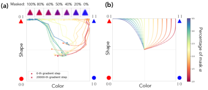
Figure 9: Underspecification hinders out-of-distribution (OOD) generalization. (a) The learning dynamics with varying levels of prompt masking, from 0% to 100%, and the generated images. At 0% masking (top right image), the model correctly produces an image of blue triangle from the prompt “blue triangle.” As the masking increases (from right to left), the images gradually shift towards the incorrect color, red. (b) The simulation of the learning dynamics under underspecification in concept space based on Eq. 2. Our toy model replicates a trained network’s learning dynamics.

Toy Model of Learning Dynamics with Underspecification. When prompts are masked (i.e., underspecification occurs), target values for the concept variables are shifted: e.g., in our setup, with no mask applied, the target directions for the class 11 is $(1,1)$. When the word “red” in “red triangle” is fully masked, the target shifts to $(0,1)$. Assuming this shift is linear with respect to the percentage of masked prompts $\alpha$, we can derive the following energy function.

$$\frac{d{\bf z}}{dt}=-\nabla_{\bf z}L,\,\,L(z_{1},z_{2})=\big{(}(1-s\alpha)-z_{1}\big{)}^{2}+\big{(}1-z_{2}\big{)}^{2}.$$ (2)

In the above, parameter $s$ represents the impact of underspecification. Fig. 9 (b) shows the simulation of model behavior in the concept space according to Eq. 2 ($s=0.01$). As the masking level increases, the target directions shift from $z_{2}=1$ in the top right corner to $z_{2}=0$ in the top left corner. Our simulated dynamics thus match well with the model’s learning dynamics shown in Fig. 9 (a).

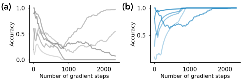
Figure 10: Underspecification and Hidden Capabilities. We use the over-prompting protocol from Sec. 4.4 to assess if the capabilities to enable OOD generalization are learned before naive input prompting. (a) Accuracy for OOD generalization across five different seed runs under naive prompting; (b) Accuracy under over-prompting, with a fixed masking percentage of 50%.

Influence of Underspecification on Emergence of Hidden Capabilities. Following Sec. 4.4, we also explore whether it is possible to elicit the desired outputs from a model trained with underspecified data. Fig. 10 shows the accuracy results over five runs (a) without using any prompting method, and (b) using over-prompting. In both scenarios, the percentage of masking is set at 50%. Results clearly demonstrate that with over-prompting, the model achieves 100% accuracy after approximately 1,000 gradient steps, whereas without over-prompting, it fails in three out of five runs even after 2,000 gradient steps. These findings confirm that capability can develop prior to observable behavior, even in cases of underspecification.

6 Discussion

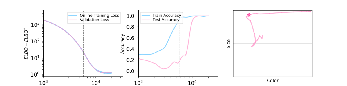
Figure 12: Loss vs. Accuracy vs. Concept Space. Loss and accuracy do not always tell the full story of what, and even more importantly when, the model is learning a capability. The star symbol in panel (c) shows point of sudden turn and concept learning, i.e., the moment when well defined prompting protocols can elicit the desired output from the model, indicating the model has learned the capability to alter a concept.

Why study the concept space? One might ask the question of why the concept space could be useful beyond synthetic datasets. In Fig. 12, we show the loss, accuracy, and training trajectory in concept space of a model from Fig. 6. The time at which the model acquires the capability to manipulate size and color independently is not evident from either the loss or accuracy curves. However, in concept space, one can directly see the divergence of the trajectory from concept memorization. Benchmarking generative models is a challenging task, still often involving humans in the loop [102, 103]. Our concept space framework suggests that benchmarking out-of-distribution (OOD) generalization can potentially be reduced to monitoring the learning trajectory in concept space.

Concept Learning vs. Grokking. We make a distinction between our delayed elicitation of capabilities versus grokking [104]. The common aspect is that the measured performance on a test set is delayed from the train set, as seen in Fig. 12. However, we deal with out-of-distribution test data, which is different from the setups like modular arithmetic or polynomial regression in which grokking is usually explored [104, 105, 106, 107, 108]. Second, work on hidden progress measures show that in fact a model is continuously building representations towards the mechanism to solve the specified task [107, 109]; however, our results find that even at the level of latent representations, there is a sudden emergence whereby the model learns the capability to manipulate concepts underlying the data-generating process and generalize OOD.

Is Concept Learning a Phase Transition?

In Sec. 4.4, we have demonstrated that before the capability to manipulate a concept is learned, the desired outputs cannot be generated irrelevant of the protocol used for prompting the model. Moreover, we showed that different protocols yield desired outputs at precisely the same time, and this time is also independent of model initialization. We thus hypothesize that: Concept learning is a well-controlled phase transition in model capability, but the ability to elicit this capability via a predefined single input prompting can be arbitrarily delayed, e.g., by the level of the concept signal.

Appendix A Experimental Details

A.1 Synthetic data

We design a data generation process (DGP) compatible with the concept space framework introduced in Sec. 3. Our full DGP has six concepts: shape=$\{\text{circle},\text{triangle}\}$, x coordinate$\in\mathbb{R}$, y coordinate$\in\mathbb{R}$, color=$\{\text{red},\text{blue}\}$, size=$\{\text{big},\text{small}\}$, and background color=$\{\text{bright},\text{dark}\}$. We generally explore only a subset of these at a given time in our experiments.

In Sec. 4, we fix shape=circle and x coordinate, y coordinate, background color are masked out. Thus the conditioning vector $h$ only specifies color=$\{\text{{red}},\text{{blue}}\}$ and size=$\{\text{{big}},\text{{small}}\}$. We sample both of these concept variables from a mixture of two uniform distributions, one component for each class (big, small) and (red, blue). Each value in each dimension is sampled from $\mathcal{U}(m^{i}-s,m^{i}+s)$, where $m^{i}$ is the class dependent mean. For example, color=red could be sampled from $\mathcal{U}(0.7,0.9)\times\mathcal{U}(0.1,0.3)\times\mathcal{U}(0.1,0.3)$, where $m^{0}=(0.8,0.2,0.2)$ For brevity, we name the four resulting classes “00”, “01”, “10”, and “11”, where the class “11” is kept as the unseen target to evaluate out-of-distribution (OOD) generalization. For each training run, the DGP was initialized with a set random seed and 2048 images were generated in each class.

In Sec. 5, we used two concept variables, shape and size. The training dataset included the classes “00”, “01”, and “10”. For evaluation, we used the class “11”. For each class, we generated a total of 1,000 images, each featuring objects of varying positions and sizes to ensure variability in our dataset.

In App. C.4, we add the concept variable background color$\in\mathbb{R}^{3}$ to have a three dimensional concept space of (color, size, background color). In this case our training data is composed of the classes (“000”, “001”, “010”, “100”) and the test classes are (“011”, “101”, “110”, “111”)

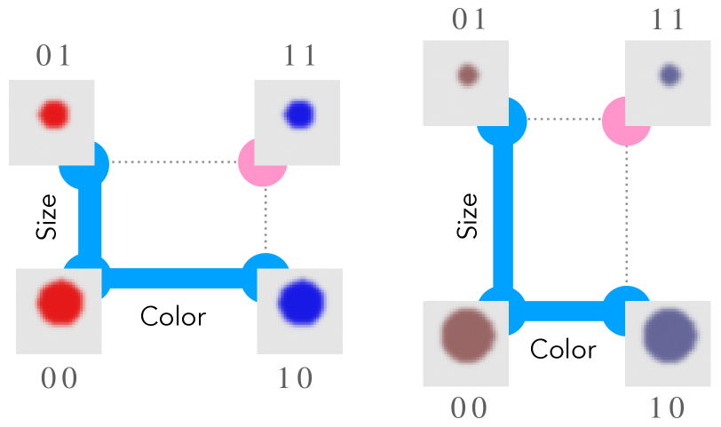
Figure 11: Different distributions in concept values result in different concept signal. (Left) The color separation between the classes is stronger than the size separations resulting in a stronger concept signal in the color dimension. (right) The size separation between the classes is stronger, thus resulting in a stronger concept signal in size

Our DGP is resolution agnostic, but we work with square images of 32x32 for fast experiments.

Adjusting concept signal To adjust concept signals, we vary the class dependent mean of the two components of the mixture distributions. For example a strong color concept signal is achieved by drawing color=red from the mean $m^{red}=(0.9,0.1,0.1)$ and color=blue from the mean $m^{blue}=(0.1,0.1,0.9)$ whereas a weak color concept signal can be drawn using $m^{red}=(0.6,0.4,0.4)$ and $m^{blue}=(0.4,0.4,0.6)$. We scale the standard deviation of each component by the same ratio the difference between the class means has been scaled. This latter is important to avoid the model’s natural interpolation or extrapolation abilities from confounding with the generalization dynamics.

Fig. 11 illustrates two datasets with varying concept signals. Fig. 11 (a) illustrates a case where the size concept signal is stronger than the color concept signal, while Fig. 11 (b) illustrates the inverse case where the color concept signal is stronger.

A.2 Model Details

Model Architecture We used a network architecture similar to the U-Net [93] used in Variational Diffusion Models [88]. We used the implementation publicly available in [110]. The architecture has 2 ResNet [111] blocks before each downsampling layer and a has self-attention layer in the bottleneck layer of the network. The U-Net has 64, 128, 256 channels at each resolution levels, an has a LayerNorm [112] and a GELU [113] activation. We used a sinusoidal timestep embedding [114] of 64 dimensions followed by a 2-layer MLP with hidden dimension 256 and a conditioning vector embedding using a 2-layer MLP with hidden dimensions 256 independent in every residual block.

Optimizer We use the AdamW [115] optimizer with learning rate $0.001$ and weight decay $0.01$ to optimize the parameters of our network. We train our networks for $20$K gradient steps. We use the default values for the decay rates: $\beta_{1}=0.9,\>\beta_{2}=0.999$.

Classifier Free Guidance At training time we drop the conditioning to a $-1.0$ filled null vector $\phi$ with probability 0.2. This choice was made as opposed to the conventional choice of dropping it to the null vector since the null vector was near the interpolation limit of our model in the color subspace of the conditioning. The $w_{cfg}$ parameter is used to estimate the noise in the diffusion process by: $\hat{\epsilon}_{t-1}=f_{\theta}(x_{t}|\phi)+w_{cfg}*(f_{\theta}(x_{t}|h)-f_{\theta}(x_{t}|\phi))$, where $\theta$ denotes parameters of the network $f$.

Diffusion Process Hyperparameters We used the continuous time variational diffusion model [88] framework to (i) keep the sampling step parameter T an inference time hyperparameter and (ii) to allow the model to the adjust its optimal noise schedule for these images, especially since our synthetic images are expected to be different in SNR from natural images. In particular, we initialize our network with $\gamma_{i}=-5.0$ and $\gamma_{f}=10.0$ (see [88] for the definition of $\gamma$) and use a learned linear schedule of $\gamma(t)$. We use a reconstruction loss corresponding to a negative log likelihood from a standard normal with $\sigma=10^{-3}$ centered at the data for the first step of the diffusion process.

Evaluation probe Details. We used a U-Net [93] backbone with 64 output channels followed by a max pooling layer and $n$ 1-layer MLP classifier for each of the $n$ classes to estimate each concept of an image independently. We sample from the same data distribution but with maximal data diversity, i.e., with $s_{i}$ values in App. A.1 maximized within the range allowing perfect classification (no overlap of $z$ between classes). We sample 4096 images per class from the DGP and train the classifier for 10K gradient steps with AdamW [115] and achieve a 100% accuracy on the held out test set. At evaluation phase, we average the classifier softmax output over 5 data generation / model initialization seeds and 32 inference samples to construct the concept space representation of the generations.

Computational Details. We implement our models in PyTorch [116]. A standard model run (e.g., in Sec. 4.2) took $\sim$ 20 minutes on a single NVIDIA A100 40GB GPU. The CelebA runs took $\sim$ 24 hours on the same GPU.

A.3 Training Procedure

The diffusion model was implemented using PyTorch and trained on four Nvidia A100 GPUs. We conducted a hyperparameter search using a validation set, testing batch sizes from 32 to 256, number of channels per layer from 64 to 512, learning rates between $10^{-4}$ and $10^{-3}$, the number of steps in the diffusion process from 100 to 400. We employed the Adam optimizer [117] with $\beta_{1}=0.9$, $\beta_{2}=0.99$, and weight decay of $10^{-5}$.

Appendix B Details on Alternative Protocols for Eliciting Model Capabilities

Input Space: Overprompting.

Our model is trained on a distribution of conditioning centered around a class dependent mean: $p^{i}(z_{j})=\mathcal{U}(m^{i}_{j}-s_{j},m^{i}_{j}+s_{j})$ for each class $i$. We prompt the model with conditioning vectors extrapolated in the direction $\vec{m_{1}}-\vec{m_{0}}$. For instance, assuming the red conditioning was $(0.6,0.4,0.4)$ and the blue conditioning was $(0.4,0.4,0.6)$, we “prompt” the model with $(0.2,0.2,0.8)$. In practice, we use 5 conditionings $(0.4,0.4,0.6)$, $(0.35,0.35,0.65)$, $(0.25,0.25,0.75)$, $(0.15,0.15,0.85)$, $(0.05,0.05,0.95)$, and report the maximum joint accuracy.

Activation Space: Linear Latent Intervention.

We demonstrate the ability to compose capabilities by manipulating the conditional vectors $\vec{h}$. Namely, we create a condition vector $\vec{h}_{i}$ for a specific concept $i$ by specifying a concept of interest (e.g., $\vec{h}_{\texttt{blue}}=M(z_{\texttt{blue}})$. During the forward pass, given $\vec{h}$, we can compute the component of each concept in $\vec{h}$ by projecting onto a specific concept-condition vector ($\vec{h}_{\texttt{blue}}$). We can then enhance or reduce the component of each concept by scaling each of these projected components. In practice, we perform the following operation: $\vec{h}^{\prime}=\vec{h}+\alpha\vec{h}_{\texttt{blue}}-\beta\vec{h}_{\texttt{large}}$, where $\alpha,\beta$ are hyperparameters. We sweep over $[0.1,1,2,4]$ for $\alpha$ and $[0.1,0.25,0.5,1]$ for $\beta$.

$\vec{h}_{\texttt{blue}}$ is constructed by first deriving a blue direction in condition embedding space ($\vec{h}_{5,5,95}$) by embedding a concept vector ($\vec{z}_{5,5,95}$) where its RGB components are set to $(0.05,0.05,0.95)$: $\vec{h}_{5,5,95}=M(\vec{z}_{5,5,95})$. We then project $\vec{h}$ onto this direction to derive $\vec{h}_{\texttt{blue}}$. $\vec{h}_{\texttt{large}}$ is generated similarly using $\vec{z}_{\text{size}=0.7}$. The model then generates an image conditioned on $\vec{h}^{\prime}$.

Appendix C Additional Results

C.1 Loss and Accuracy versus Concept Space

We plot loss, accuracy, and training trajectory in concept space of the models from Fig. 6. The time at which the model acquires a capability to manipulate the concept color is not evident from the loss or accuracy curves; however, in concept space, it is evident that the concept is learned together with the departure from concept memorization. Benchmarking generative models is a challenging task, still often involving humans in the loop [102, 103]. Our concept space framework suggests that benchmarking out-of-distribution (OOD) generalization can potentially be reduced to monitoring the learning trajectory in concept space.

C.2 Additional trajectories of learning dynamics (Fig. 13)

Here we show all concept space trajectories for the experiments mentioned in Fig. 4 (a,b), for all classes and color concept signal levels. We find asymmetric behavior for the 01 class and the 10 class when adjusting the color concept signal level. The dynamics of the generations in the training set matches our intuitions. At low color concept signal, we observe that the dynamics fit the size for both 00 and 10, and diverge towards their correct colors.

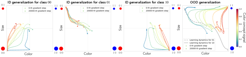
Figure 13: Concept Space Dynamics for all classes (00, 01, 10, 11). The experiment is identical as in Fig. 4. The [0,1) normalized color concept signal is color coded in every trajectory. Two training data trajectories are shown in gray in the last panel to show concept memorization.

C.3 Experiments with real data: CelebA

To assess our findings on a more realistic dataset, we ran experiments on the CelebA [118] dataset. We selected the Not Male and Smiling features as the two concept dimensions to explore. This choice was motivated by the relatively balanced number of samples in all four classes(00=(Male, Not Smiling), 01=(Male, Smiling), 10=(Not Male, Not Smiling), 11=(Not Male, Smiling)), from which we randomly sampled 30K images in each class. To construct the concept space, we trained a fully convolutional network with a average pooling layer followed by a classification MLP head to classify the two attributes with independent cross entropy losses. (See A.2). We trained the classifier with the AdamW [115] optimizer with learning rate $10^{-3}$ and weight decay $10^{-5}$ for 10K gradient steps. The classifier achieved a final accuracy of respectively $95\%$ and $97\%$ on the held out validation set, which was $10\%$ of the entire dataset.

We trained the same diffusion model (See App. A.2) from our synthetic experiments on 64x64 resized images from the classes (00, 01, 10) and assessed the out-of-distribution (OOD) generalization to 11. We used a color jitter of 0.1 for brightness, contrast and saturation and randomly flipped the images horizontally. As the class attributes are categorical, they were one hot encoded and concatenated to an input conditioning vector of 4 dimensions. The diffusion model was trained for $10^{6}$ gradient steps with a batch size of 64 with the same optimizer as in the main experiments.

The concept space dynamics of generations from the in distribution conditioning and OOD conditioning are shown in Fig. 14. We find similar observations from the concept space trajectories as in our synthetic experiments. Initially, the images corresponding to the class 11 follows the concept space trajectory of 10, optimizing Not Male, which we intuitively expect to have a stronger concept signal, although it is intractable to compute since the DGP is unknown. Similar to our synthetic experiments, we see a transition in the concept space trajectory of the compositional class corresponding to the model disentangling the concepts. After this transition, concept learning begins but we see biases, where we see a trade-off of moving in the right direction towards one concept degrades the other one as seen in Fig. 4 (b). The visual generations in Fig. 14 confirm that our findings are not merely a result of an ill-calibrated classifier model. However, in this case, we do not observe full out-of-distribution (OOD) generalization at 1M gradient steps. We expect this task of generating (NOT Male, Smiling) is inherently harder than our synthetic setup. We note that the goal of this experiment is not to show good compositional generalization but it is more on confirming that our qualitative findings generalize to real data without touching the model or training method.

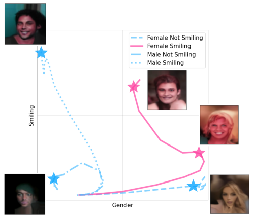
Figure 14: Concept Space Dynamics in CelebA. We train on the classes 00=$(\text{Male},\text{NOT Smiling})$, 01=$(\text{Male},\text{Smiling})$, 10=$(\text{NOT Male},\text{NOT Smiling})$ (plotted in blue) and test on the class 10=$(\text{NOT Male},\text{Smiling})$ (plotted in pink). We find similar observations as in Fig. 4.2, concept memorization and the resulting bias.

C.4 Experiments with 3D concept space (Fig. 15)

To further verify our findings in Sec. 4, we explore a setup where the concept conditioning specifies three concepts: color, size and background color. Fig. 15 illustrates two example scenarios in which the concept signal in color and background color are varied, respectively resulting in cases of success and failure of OOD generalization. The length of edges of the cuboids represent their concept signal magnitude. In Fig. 15 (a), we see that the object color has a strong concept signal and this is reflected in the concept space trajectories as this direction being split first. In this case we see, similar to the blue generalization curve in Fig. 4 (b) and Fig. 13 (rightmost panel), a slow generalization process for the compositional class 111. Similarly to our findings in Sec. 4.2, we observe that the 011 class initially undergoes concept memorization for class 010, which shares the two stronger concept signals color and background color, and shows a transition where it leaves this phase. In Fig. 15 (b), we see a case where out-of-distribution (OOD) generalization did not succeed within the given 80K gradient steps. In this case, we see two classes, 011 and 111, which are not correctly learned, and thus suspect that the model did not learn to generalize the background color. However, the concept space trajectories suggest that the capability is present.

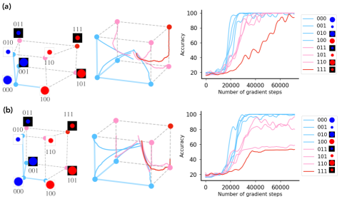
Figure 15: Concept Learning Geometry underlies emergence Success and Failure modes of out-of-distribution (OOD) generalization. (a) A success case where color carries the strongest concept signal. We see aspects of concept memorization from the class 011. (b) A failure case where the background color didn’t generalize. In this case, the model does not produce the right background color while the concept space suggest that this capability is present.

C.5 Experiments with classifier free guidance

An implication of our conclusions in Sec. 4.4 is that before the model has passed the transition point where the model has the capability to compose concepts, the model should not be able to generate small blue circles no matter how well “prompted”. Here, instead of prompting, we explore Classifier Free Guidance (CFG) [95] to see if our findings apply to a conditional diffusion model trained with CFG. In Fig. 16, we see that even the models with CFG show this transition from concept memorization to out-of-distribution (OOD) generalization. In a scenario where there isn’t a sharp acquisition of the capability to compositionally generalize, we would expect the sharp transition to disappear with CFG scale.

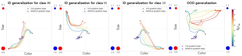
Figure 16: Learning Dynamics in Concept space for Classifier-free Guidance We show the learning dynamics in the concept space for all the classes (00, 01, 10, 11). The generalization task (rightmost) shows a sharp transition from concept memorization to out-of-distribution (OOD) generalization independently of the Classifier-Free Guidance (CFG) scale.

C.6 Patching the embedding module

Assuming a model does not have the capability to generate images from an OOD concept class, we simply swap the embedding module for processing the conditioning vector $h$ with that of the last checkpoint. One possible interpretation for this method is that the embedding module disentangles the concepts, i.e., generates a representation for each concept, while the U-Net [93] then utilizes such representations. This would imply that the U-Net [93] already learns how to utilize concept representations early during training, while further gradient steps lead to more robust concept representations.

We test our approach on 5 random initialization seeds. Results are shown in Fig. 17 and we find that for some seeds, we are able to elicit the target behavior at around the same time in which overprompting and linear interventions also elicit the target behavior; for other seeds, this is not the case. Interestingly, we find that our method works well for seeds with “stable” learning dynamics, in that once the model reaches $\sim 100\%$ accuracy, it converges and stays at such accuracy, while some seeds have “unstable” learning dynamics in that their accuracies oscillate.

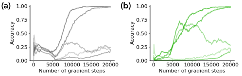
Figure 17: Embedding patching. We patch the embedding module (an MLP) used for transforming the conditioning information into an embedding that the model processes from the last checkpoint to intermediate checkpoints. Panel (a) shows the baseline accuracy for out-of-distribution (OOD) generalization across five different seed runs, while panel (b) shows accuracy achieved when the patched embedding module is used.

References

- Kawar et al. [2022] Bahjat Kawar, Shiran Zada, Oran Lang, Omer Tov, Huiwen Chang, Tali Dekel, Inbar Mosseri, and Michal Irani. Imagic: Text-based real image editing with diffusion models. arXiv preprint arXiv:2210.09276, 2022.
- Brooks et al. [2024] Tim Brooks, Bill Peebles, Connor Holmes, Will DePue, Yufei Guo, Li Jing, David Schnurr, Joe Taylor, Troy Luhman, Eric Luhman, Clarence Ng, Ricky Wang, and Aditya Ramesh. Video generation models as world simulators. 2024. URL https://openai.com/research/video-generation-models-as-world-simulators.
- Kondratyuk et al. [2023] Dan Kondratyuk, Lijun Yu, Xiuye Gu, José Lezama, Jonathan Huang, Rachel Hornung, Hartwig Adam, Hassan Akbari, Yair Alon, Vighnesh Birodkar, et al. Videopoet: A large language model for zero-shot video generation. arXiv preprint arXiv:2312.14125, 2023.
- Ho et al. [2022] Jonathan Ho, William Chan, Chitwan Saharia, Jay Whang, Ruiqi Gao, Alexey Gritsenko, Diederik P Kingma, Ben Poole, Mohammad Norouzi, David J Fleet, et al. Imagen video: High definition video generation with diffusion models. arXiv preprint arXiv:2210.02303, 2022.
- Saharia et al. [2022a] Chitwan Saharia, Jonathan Ho, William Chan, Tim Salimans, David J Fleet, and Mohammad Norouzi. Image super-resolution via iterative refinement. IEEE Transactions on Pattern Analysis and Machine Intelligence, 2022a.
- Poole et al. [2022] Ben Poole, Ajay Jain, Jonathan T Barron, and Ben Mildenhall. Dreamfusion: Text-to-3d using 2d diffusion. arXiv preprint arXiv:2209.14988, 2022.
- Gao et al. [2024] Ruiqi Gao, Aleksander Holynski, Philipp Henzler, Arthur Brussee, Ricardo Martin-Brualla, Pratul Srinivasan, Jonathan T Barron, and Ben Poole. Cat3d: Create anything in 3d with multi-view diffusion models. arXiv preprint arXiv:2405.10314, 2024.
- Chen et al. [2024] Ziyang Chen, Daniel Geng, and Andrew Owens. Images that sound: Composing images and sounds on a single canvas. arXiv preprint arXiv:2405.12221, 2024.
- Du et al. [2023a] Yilun Du, Mengjiao Yang, Bo Dai, Hanjun Dai, Ofir Nachum, Joshua B Tenenbaum, Dale Schuurmans, and Pieter Abbeel. Learning universal policies via text-guided video generation. arXiv e-prints, pages arXiv–2302, 2023a.
- Du et al. [2023b] Yilun Du, Mengjiao Yang, Pete Florence, Fei Xia, Ayzaan Wahid, Brian Ichter, Pierre Sermanet, Tianhe Yu, Pieter Abbeel, Joshua B Tenenbaum, et al. Video language planning. arXiv preprint arXiv:2310.10625, 2023b.
- Bruce et al. [2024] Jake Bruce, Michael Dennis, Ashley Edwards, Jack Parker-Holder, Yuge Shi, Edward Hughes, Matthew Lai, Aditi Mavalankar, Richie Steigerwald, Chris Apps, et al. Genie: Generative interactive environments. arXiv preprint arXiv:2402.15391, 2024.
- Khanna et al. [2023] Samar Khanna, Patrick Liu, Linqi Zhou, Chenlin Meng, Robin Rombach, Marshall Burke, David Lobell, and Stefano Ermon. Diffusionsat: A generative foundation model for satellite imagery. arXiv preprint arXiv:2312.03606, 2023.
- Times) [2024] Yan Zhuang (New York Times). Imran Khan’s ‘Victory Speech’ From Jail Shows A.I.’s Peril and Promise, 2024. https://www.nytimes.com/2024/02/11/world/asia/imran-khan-artificial-intelligence-pakistan.html.
- [14] Mark Sullivan (FastCompany). AI deepfakes get very real as 2024 election season begins, 2024. https://www.fastcompany.com/91020077/ai-deepfakes-taylor-swift-joe-biden-2024-election.
- Bubeck et al. [2023] Sébastien Bubeck, Varun Chandrasekaran, Ronen Eldan, Johannes Gehrke, Eric Horvitz, Ece Kamar, Peter Lee, Yin Tat Lee, Yuanzhi Li, Scott Lundberg, et al. Sparks of artificial general intelligence: Early experiments with gpt-4. arXiv preprint arXiv:2303.12712, 2023.
- Gemini Team [2024] Gemini Team. Gemini 1.5: Unlocking multimodal understanding across millions of tokens of context. Technical report, Google DeepMind, 2024. https://storage.googleapis.com/deepmind-media/gemini/gemini_v1_5_report.pdf.
- OpenAI [2023] OpenAI. GPT-4 System Card. Technical report, OpenAI, 2023. https://cdn.openai.com/papers/gpt-4-system-card.pdf.
- Claude team [2024] Claude team. Introducing the next generation of Claude. Technical report, Anthropic AI, 2024. https://www.anthropic.com/news/claude-3-family.
- Deepmind) [2024] Generative Media Team (Google Deepmind). Generating audio for video, 2024. https://deepmind.google/discover/blog/generating-audio-for-video/.
- Liu et al. [2023a] Shengchao Liu, Yanjing Li, Zhuoxinran Li, Anthony Gitter, Yutao Zhu, Jiarui Lu, Zhao Xu, Weili Nie, Arvind Ramanathan, Chaowei Xiao, et al. A text-guided protein design framework. arXiv preprint arXiv:2302.04611, 2023a.
- News [2024] MIT News. Speeding up drug discovery with diffusion generative models, 2024. https://news.mit.edu/2023/speeding-drug-discovery-with-diffusion-generative-models-diffdock-0331.
- Bengio et al. [2013] Yoshua Bengio, Aaron Courville, and Pascal Vincent. Representation learning: A review and new perspectives. IEEE transactions on pattern analysis and machine intelligence, 35(8):1798–1828, 2013.
- Locatello et al. [2019] Francesco Locatello, Stefan Bauer, Mario Lucic, Gunnar Raetsch, Sylvain Gelly, Bernhard Schölkopf, and Olivier Bachem. Challenging common assumptions in the unsupervised learning of disentangled representations. In Proc. int. conf. on machine learning (ICML), 2019.
- Kaur et al. [2022] Jivat Neet Kaur, Emre Kiciman, and Amit Sharma. Modeling the data-generating process is necessary for out-of-distribution generalization. arXiv preprint. arXiv:2206.07837, 2022.
- Jiang et al. [2021] Liwei Jiang, Jena D Hwang, Chandra Bhagavatula, Ronan Le Bras, Jenny Liang, Jesse Dodge, Keisuke Sakaguchi, Maxwell Forbes, Jon Borchardt, Saadia Gabriel, et al. Can machines learn morality? the delphi experiment. arXiv e-prints, pages arXiv–2110, 2021.
- Schölkopf et al. [2021] Bernhard Schölkopf, Francesco Locatello, Stefan Bauer, Nan Rosemary Ke, Nal Kalchbrenner, Anirudh Goyal, and Yoshua Bengio. Towards causal representation learning. arXiv preprint. arXiv:2102.11107, 2021.
- Peters et al. [2017] Jonas Peters, Dominik Janzing, and Bernhard Schölkopf. Elements of causal inference: foundations and learning algorithms. The MIT Press, 2017.
- Kaddour et al. [2022] Jean Kaddour, Aengus Lynch, Qi Liu, Matt J Kusner, and Ricardo Silva. Causal machine learning: A survey and open problems. arXiv preprint arXiv:2206.15475, 2022.
- Ramesh et al. [2022] Aditya Ramesh, Prafulla Dhariwal, Alex Nichol, Casey Chu, and Mark Chen. Hierarchical text-conditional image generation with clip latents. arXiv preprint arXiv:2204.06125, 2022.
- Okawa et al. [2024] Maya Okawa, Ekdeep Singh Lubana, Robert P. Dick, and Hidenori Tanaka. Compositional abilities emerge multiplicatively: Exploring diffusion models on a synthetic task, 2024.
- Yu et al. [2024] Hu Yu, Hao Luo, Fan Wang, and Feng Zhao. Uncovering the text embedding in text-to-image diffusion models. arXiv preprint arXiv:2404.01154, 2024.
- Kong et al. [2024] Lingjing Kong, Guangyi Chen, Biwei Huang, Eric P Xing, Yuejie Chi, and Kun Zhang. Learning discrete concepts in latent hierarchical models. arXiv preprint arXiv:2406.00519, 2024.
- Wu et al. [2023] Qiucheng Wu, Yujian Liu, Handong Zhao, Ajinkya Kale, Trung Bui, Tong Yu, Zhe Lin, Yang Zhang, and Shiyu Chang. Uncovering the disentanglement capability in text-to-image diffusion models. In Proceedings of the IEEE/CVF Conference on Computer Vision and Pattern Recognition, pages 1900–1910, 2023.
- Gandikota et al. [2023] Rohit Gandikota, Joanna Materzynska, Tingrui Zhou, Antonio Torralba, and David Bau. Concept sliders: Lora adaptors for precise control in diffusion models. arXiv preprint arXiv:2311.12092, 2023.
- Liu et al. [2023b] Nan Liu, Yilun Du, Shuang Li, Joshua B Tenenbaum, and Antonio Torralba. Unsupervised compositional concepts discovery with text-to-image generative models. In Proceedings of the IEEE/CVF International Conference on Computer Vision, pages 2085–2095, 2023b.
- Besserve et al. [2018] Michel Besserve, Arash Mehrjou, Rémy Sun, and Bernhard Schölkopf. Counterfactuals uncover the modular structure of deep generative models. arXiv preprint. arXiv:1812.03253, 2018.
- Wang et al. [2024] Zihao Wang, Lin Gui, Jeffrey Negrea, and Victor Veitch. Concept algebra for (score-based) text-controlled generative models. Advances in Neural Information Processing Systems, 36, 2024.
- Udandarao et al. [2024] Vishaal Udandarao, Ameya Prabhu, Adhiraj Ghosh, Yash Sharma, Philip HS Torr, Adel Bibi, Samuel Albanie, and Matthias Bethge. No" zero-shot" without exponential data: Pretraining concept frequency determines multimodal model performance. arXiv preprint arXiv:2404.04125, 2024.
- Conwell and Ullman [2022] Colin Conwell and Tomer Ullman. Testing relational understanding in text-guided image generation. arXiv preprint arXiv:2208.00005, 2022.
- Conwell and Ullman [2023] Colin Conwell and Tomer Ullman. A comprehensive benchmark of human-like relational reasoning for text-to-image foundation models. In ICLR 2023 Workshop on Mathematical and Empirical Understanding of Foundation Models, 2023.
- Leivada et al. [2022] Evelina Leivada, Elliot Murphy, and Gary Marcus. Dall-e 2 fails to reliably capture common syntactic processes. arXiv preprint arXiv:2210.12889, 2022.
- Gokhale et al. [2022] Tejas Gokhale, Hamid Palangi, Besmira Nushi, Vibhav Vineet, Eric Horvitz, Ece Kamar, Chitta Baral, and Yezhou Yang. Benchmarking spatial relationships in text-to-image generation. arXiv preprint arXiv:2212.10015, 2022.
- Singh et al. [2021] Gautam Singh, Fei Deng, and Sungjin Ahn. Illiterate dall-e learns to compose. arXiv preprint arXiv:2110.11405, 2021.
- Rassin et al. [2022] Royi Rassin, Shauli Ravfogel, and Yoav Goldberg. Dalle-2 is seeing double: flaws in word-to-concept mapping in text2image models. arXiv preprint arXiv:2210.10606, 2022.
- Yu et al. [2022] Jiahui Yu, Yuanzhong Xu, Jing Yu Koh, Thang Luong, Gunjan Baid, Zirui Wang, Vijay Vasudevan, Alexander Ku, Yinfei Yang, Burcu Karagol Ayan, et al. Scaling autoregressive models for content-rich text-to-image generation. arXiv preprint arXiv:2206.10789, 2022.
- Li et al. [2024] Hao Li, Yang Zou, Ying Wang, Orchid Majumder, Yusheng Xie, R Manmatha, Ashwin Swaminathan, Zhuowen Tu, Stefano Ermon, and Stefano Soatto. On the scalability of diffusion-based text-to-image generation. arXiv preprint arXiv:2404.02883, 2024.
- Millière and Buckner [2024] Raphaël Millière and Cameron Buckner. A philosophical introduction to language models – part i: Continuity with classic debates, 2024.
- Millière and Buckner [2024] Raphaël Millière and Cameron Buckner. A philosophical introduction to language models-part ii: The way forward. arXiv preprint arXiv:2405.03207, 2024.
- Kojima et al. [2022] Takeshi Kojima, Shixiang (Shane) Gu, Machel Reid, Yutaka Matsuo, and Yusuke Iwasawa. Large language models are zero-shot reasoners. In Advances in Neural Information Processing Systems, volume 35, 2022.
- Wei et al. [2022] Jason Wei, Xuezhi Wang, Dale Schuurmans, Maarten Bosma, Ed Chi, Quoc Le, and Denny Zhou. Chain of thought prompting elicits reasoning in large language models. arXiv preprint arXiv:2201.11903, 2022.
- Hubinger et al. [2024] Evan Hubinger, Carson Denison, Jesse Mu, Mike Lambert, Meg Tong, Monte MacDiarmid, Tamera Lanham, Daniel M Ziegler, Tim Maxwell, Newton Cheng, et al. Sleeper agents: Training deceptive llms that persist through safety training. arXiv preprint arXiv:2401.05566, 2024.
- Kwon et al. [2023] Mingi Kwon, Jaeseok Jeong, and Youngjung Uh. Diffusion models already have a semantic latent space. In The Eleventh International Conference on Learning Representations, 2023. URL https://openreview.net/forum?id=pd1P2eUBVfq.
- Bubeck [2023] Sébastien Bubeck. Sparks of artificial general intelligence: Early experiments with GPT-4 (Talk), 2023. URL https://www.youtube.com/watch?v=qbIk7-JPB2c.
- Kim and Mnih [2018] Hyunjik Kim and Andriy Mnih. Disentangling by factorising. In International Conference on Machine Learning, pages 2649–2658. PMLR, 2018.
- Van Steenkiste et al. [2019] Sjoerd Van Steenkiste, Francesco Locatello, Jürgen Schmidhuber, and Olivier Bachem. Are disentangled representations helpful for abstract visual reasoning? Adv. in Neural Information Processing Systems (NeurIPS), 2019.
- Hyvarinen and Morioka [2017] Aapo Hyvarinen and Hiroshi Morioka. Nonlinear ICA of temporally dependent stationary sources. In Proc. Int. Conf. on Artificial Intelligence and Statistics (AISTATS), 2017.
- Hyvarinen and Morioka [2016] Aapo Hyvarinen and Hiroshi Morioka. Unsupervised feature extraction by time-contrastive learning and nonlinear ica. Adv. in Neural Information Processing Systems (NeurIPS), 2016.
- Hyvarinen et al. [2019] Aapo Hyvarinen, Hiroaki Sasaki, and Richard Turner. Nonlinear ICA using auxiliary variables and generalized contrastive learning. In The 22nd Int. Conf. on Artificial Intelligence and Statistics (AISTATS), 2019.
- Von Kügelgen et al. [2021] Julius Von Kügelgen, Yash Sharma, Luigi Gresele, Wieland Brendel, Bernhard Schölkopf, Michel Besserve, and Francesco Locatello. Self-supervised learning with data augmentations provably isolates content from style. Adv. in Neural Information Processing Systems (NeurIPS), 2021.
- Gresele et al. [2021] Luigi Gresele, Julius Von Kügelgen, Vincent Stimper, Bernhard Schölkopf, and Michel Besserve. Independent mechanism analysis, a new concept? Adv. in Neural Information Processing Systems (NeurIPS), 2021.
- Carey [2000] Susan Carey. The origin of concepts. Journal of Cognition and Development, 1(1):37–41, 2000.
- Carey [1991] Susan Carey. Knowledge acquisition: Enrichment or conceptual change. The epigenesis of mind: Essays on biology and cognition, pages 257–291, 1991.
- Carey [1992] Susan Carey. The origin and evolution of everyday concepts. Cognitive models of science, 15:89–128, 1992.
- Carey and Spelke [1994] Susan Carey and Elizabeth Spelke. Domain-specific knowledge and conceptual change. Mapping the mind: Domain specificity in cognition and culture, 169:200, 1994.
- Carey [2004] Susan Carey. Bootstrapping & the origin of concepts. Daedalus, 133(1):59–68, 2004.
- Carey [2009] Susan Carey. Where our number concepts come from. The Journal of philosophy, 106(4):220, 2009.
- Marks and Tegmark [2023] Samuel Marks and Max Tegmark. The geometry of truth: Emergent linear structure in large language model representations of true/false datasets. arXiv preprint arXiv:2310.06824, 2023.
- Marks et al. [2024] Samuel Marks, Can Rager, Eric J Michaud, Yonatan Belinkov, David Bau, and Aaron Mueller. Sparse feature circuits: Discovering and editing interpretable causal graphs in language models. arXiv preprint arXiv:2403.19647, 2024.
- Gurnee et al. [2023] Wes Gurnee, Neel Nanda, Matthew Pauly, Katherine Harvey, Dmitrii Troitskii, and Dimitris Bertsimas. Finding neurons in a haystack: Case studies with sparse probing. arXiv preprint arXiv:2305.01610, 2023.
- Gurnee and Tegmark [2023] Wes Gurnee and Max Tegmark. Language models represent space and time. arXiv preprint arXiv:2310.02207, 2023.
- Arditi et al. [2024] Andy Arditi, Oscar Obeso, Aaquib Syed, Daniel Paleka, Nina Rimsky, Wes Gurnee, and Neel Nanda. Refusal in language models is mediated by a single direction. arXiv preprint arXiv:2406.11717, 2024.
- Halawi et al. [2023] Danny Halawi, Jean-Stanislas Denain, and Jacob Steinhardt. Overthinking the truth: Understanding how language models process false demonstrations. arXiv preprint arXiv:2307.09476, 2023.
- Haas et al. [2023] René Haas, Inbar Huberman-Spiegelglas, Rotem Mulayoff, and Tomer Michaeli. Discovering interpretable directions in the semantic latent space of diffusion models. arXiv preprint arXiv:2303.11073, 2023.
- Park et al. [2023a] Yong-Hyun Park, Mingi Kwon, Junghyo Jo, and Youngjung Uh. Unsupervised discovery of semantic latent directions in diffusion models. arXiv preprint arXiv:2302.12469, 2023a.
- Basu et al. [2024] Samyadeep Basu, Keivan Rezaei, Ryan Rossi, Cherry Zhao, Vlad Morariu, Varun Manjunatha, and Soheil Feizi. On mechanistic knowledge localization in text-to-image generative models. arXiv preprint arXiv:2405.01008, 2024.
- Chen et al. [2023a] Yida Chen, Fernanda Viégas, and Martin Wattenberg. Beyond surface statistics: Scene representations in a latent diffusion model. arXiv preprint arXiv:2306.05720, 2023a.
- El Banani et al. [2024] Mohamed El Banani, Amit Raj, Kevis-Kokitsi Maninis, Abhishek Kar, Yuanzhen Li, Michael Rubinstein, Deqing Sun, Leonidas Guibas, Justin Johnson, and Varun Jampani. Probing the 3d awareness of visual foundation models. In Proceedings of the IEEE/CVF Conference on Computer Vision and Pattern Recognition, pages 21795–21806, 2024.
- Chomsky [2014] Noam Chomsky. Aspects of the Theory of Syntax. Number 11. MIT press, 2014.
- Collins [2007] John Collins. Linguistic competence without knowledge of language. Philosophy Compass, 2(6):880–895, 2007.
- De Villiers and De Villiers [1974] Jill G De Villiers and Peter A De Villiers. Competence and performance in child language: Are children really competent to judge? Journal of Child Language, 1(1):11–22, 1974.
- Brown et al. [1996] Gillian Brown, Kirsten Malmkjær, and John Williams. Performance and competence in second language acquisition. Cambridge university press, 1996.
- METR [2024] METR. Guidelines for Capabilities Elicitation, 2024. https://metr.github.io/autonomy-evals-guide/elicitation-protocol/.
- Greenblatt et al. [2024] Ryan Greenblatt, Fabien Roger, Dmitrii Krasheninnikov, and David Krueger. Stress-testing capability elicitation with password-locked models. arXiv preprint arXiv:2405.19550, 2024.
- Davidson et al. [2023] Tom Davidson, Jean-Stanislas Denain, Pablo Villalobos, and Guillem Bas. Ai capabilities can be significantly improved without expensive retraining. arXiv preprint arXiv:2312.07413, 2023.
- Casper et al. [2024] Stephen Casper, Carson Ezell, Charlotte Siegmann, Noam Kolt, Taylor Lynn Curtis, Benjamin Bucknall, Andreas Haupt, Kevin Wei, Jérémy Scheurer, Marius Hobbhahn, et al. Black-box access is insufficient for rigorous ai audits. In The 2024 ACM Conference on Fairness, Accountability, and Transparency, pages 2254–2272, 2024.
- Srivastava et al. [2022] Aarohi Srivastava, Abhinav Rastogi, Abhishek Rao, Abu Awal Md Shoeb, Abubakar Abid, Adam Fisch, Adam R Brown, Adam Santoro, Aditya Gupta, Adrià Garriga-Alonso, et al. Beyond the imitation game: Quantifying and extrapolating the capabilities of language models. arXiv preprint arXiv:2206.04615, 2022.
- Suzgun et al. [2022] Mirac Suzgun, Nathan Scales, Nathanael Schärli, Sebastian Gehrmann, Yi Tay, Hyung Won Chung, Aakanksha Chowdhery, Quoc V Le, Ed H Chi, Denny Zhou, et al. Challenging big-bench tasks and whether chain-of-thought can solve them. arXiv preprint arXiv:2210.09261, 2022.
- Kingma et al. [2023] Diederik P. Kingma, Tim Salimans, Ben Poole, and Jonathan Ho. Variational diffusion models, 2023.
- Higgins et al. [2017] Irina Higgins, Loic Matthey, Arka Pal, Christopher Burgess, Xavier Glorot, Matthew Botvinick, Shakir Mohamed, and Alexander Lerchner. beta-vae: Learning basic visual concepts with a constrained variational framework. In Proc. Int. Conf. on Learning Representations (ICLR), 2017.
- Eastwood and Williams [2018] Cian Eastwood and Christopher KI Williams. A framework for the quantitative evaluation of disentangled representations. In International Conference on Learning Representations, 2018.
- Chen et al. [2018] Ricky TQ Chen, Xuechen Li, Roger B Grosse, and David K Duvenaud. Isolating sources of disentanglement in variational autoencoders. Advances in neural information processing systems, 31, 2018.
- Kumar et al. [2017] Abhishek Kumar, Prasanna Sattigeri, and Avinash Balakrishnan. Variational inference of disentangled latent concepts from unlabeled observations. arXiv preprint arXiv:1711.00848, 2017.
- Ronneberger et al. [2015] Olaf Ronneberger, Philipp Fischer, and Thomas Brox. U-net: Convolutional networks for biomedical image segmentation, 2015.
- Kang et al. [2024] Katie Kang, Eric Wallace, Claire Tomlin, Aviral Kumar, and Sergey Levine. Unfamiliar finetuning examples control how language models hallucinate. arXiv preprint arXiv:2403.05612, 2024.
- Ho and Salimans [2022] Jonathan Ho and Tim Salimans. Classifier-free diffusion guidance. arXiv preprint arXiv:2207.12598, 2022.
- Hutchinson et al. [2022] Ben Hutchinson, Jason Baldridge, and Vinodkumar Prabhakaran. Underspecification in scene description-to-depiction tasks, 2022.
- D’Amour et al. [2022] Alexander D’Amour, Katherine Heller, Dan Moldovan, Ben Adlam, Babak Alipanahi, Alex Beutel, Christina Chen, Jonathan Deaton, Jacob Eisenstein, Matthew D Hoffman, et al. Underspecification presents challenges for credibility in modern machine learning. Journal of Machine Learning Research, 23(226):1–61, 2022.
- [98] Sandro Pezzelle. Dealing with semantic underspecification in multimodal nlp. In Proceedings of the 61st Annual Meeting of the Association for Computational Linguistics (Volume 1: Long Papers).
- Tang et al. [2023] Yingtian Tang, Yutaro Yamada, Yoyo Zhang, and Ilker Yildirim. When are lemons purple? the concept association bias of vision-language models. In Proceedings of the 2023 Conference on Empirical Methods in Natural Language Processing, 2023.
- Rassin et al. [2023] Royi Rassin, Eran Hirsch, Daniel Glickman, Shauli Ravfogel, Yoav Goldberg, and Gal Chechik. Linguistic binding in diffusion models: Enhancing attribute correspondence through attention map alignment. In Thirty-seventh Conference on Neural Information Processing Systems, 2023. URL https://openreview.net/forum?id=AOKU4nRw1W.
- Chen et al. [2023b] Junsong Chen, Jincheng Yu, Chongjian Ge, Lewei Yao, Enze Xie, Yue Wu, Zhongdao Wang, James Kwok, Ping Luo, Huchuan Lu, and Zhenguo Li. Pixart-: Fast training of diffusion transformer for photorealistic text-to-image synthesis, 2023b.
- Zhou et al. [2019] Sharon Zhou, Mitchell L. Gordon, Ranjay Krishna, Austin Narcomey, Li Fei-Fei, and Michael S. Bernstein. Hype: A benchmark for human eye perceptual evaluation of generative models, 2019.
- Saharia et al. [2022b] Chitwan Saharia, William Chan, Saurabh Saxena, Lala Li, Jay Whang, Emily Denton, Seyed Kamyar Seyed Ghasemipour, Burcu Karagol Ayan, S. Sara Mahdavi, Rapha Gontijo Lopes, Tim Salimans, Jonathan Ho, David J Fleet, and Mohammad Norouzi. Photorealistic text-to-image diffusion models with deep language understanding, 2022b.
- Power et al. [2022] Alethea Power, Yuri Burda, Harri Edwards, Igor Babuschkin, and Vedant Misra. Grokking: Generalization beyond overfitting on small algorithmic datasets. arXiv preprint arXiv:2201.02177, 2022.
- Liu et al. [2022a] Ziming Liu, Ouail Kitouni, Niklas S Nolte, Eric Michaud, Max Tegmark, and Mike Williams. Towards understanding grokking: An effective theory of representation learning. Advances in Neural Information Processing Systems, 35:34651–34663, 2022a.
- Liu et al. [2022b] Ziming Liu, Eric J Michaud, and Max Tegmark. Omnigrok: Grokking beyond algorithmic data. In The Eleventh International Conference on Learning Representations, 2022b.
- Nanda et al. [2023] Neel Nanda, Lawrence Chan, Tom Lieberum, Jess Smith, and Jacob Steinhardt. Progress measures for grokking via mechanistic interpretability, 2023.
- Kumar et al. [2023] Tanishq Kumar, Blake Bordelon, Samuel J Gershman, and Cengiz Pehlevan. Grokking as the transition from lazy to rich training dynamics. arXiv preprint arXiv:2310.06110, 2023.
- Barak et al. [2022] Boaz Barak, Benjamin Edelman, Surbhi Goel, Sham Kakade, Eran Malach, and Cyril Zhang. Hidden progress in deep learning: Sgd learns parities near the computational limit. Advances in Neural Information Processing Systems, 35:21750–21764, 2022.
- Park et al. [2023b] Core Francisco Park, Victoria Ono, Nayantara Mudur, Yueying Ni, and Carolina Cuesta-Lazaro. Probabilistic reconstruction of dark matter fields from biased tracers using diffusion models, 2023b.
- He et al. [2015] Kaiming He, Xiangyu Zhang, Shaoqing Ren, and Jian Sun. Deep residual learning for image recognition, 2015.
- Ba et al. [2016] Jimmy Lei Ba, Jamie Ryan Kiros, and Geoffrey E. Hinton. Layer normalization, 2016.
- Hendrycks and Gimpel [2023] Dan Hendrycks and Kevin Gimpel. Gaussian error linear units (gelus), 2023.
- Vaswani et al. [2023] Ashish Vaswani, Noam Shazeer, Niki Parmar, Jakob Uszkoreit, Llion Jones, Aidan N. Gomez, Lukasz Kaiser, and Illia Polosukhin. Attention is all you need, 2023.
- Loshchilov and Hutter [2019] Ilya Loshchilov and Frank Hutter. Decoupled weight decay regularization, 2019.
- Paszke et al. [2019] Adam Paszke, Sam Gross, Francisco Massa, Adam Lerer, James Bradbury, Gregory Chanan, Trevor Killeen, Zeming Lin, Natalia Gimelshein, Luca Antiga, Alban Desmaison, Andreas Köpf, Edward Yang, Zach DeVito, Martin Raison, Alykhan Tejani, Sasank Chilamkurthy, Benoit Steiner, Lu Fang, Junjie Bai, and Soumith Chintala. Pytorch: An imperative style, high-performance deep learning library, 2019.
- Kingma and Ba [2015] Diederik P Kingma and Jimmy Ba. Adam: A method for stochastic optimization. In ICLR, 2015.
- Liu et al. [2015] Ziwei Liu, Ping Luo, Xiaogang Wang, and Xiaoou Tang. Deep learning face attributes in the wild. In Proceedings of International Conference on Computer Vision (ICCV), December 2015.