Rational Empirical Interpolation Methods with Applications

Abstract

We present a rational empirical interpolation method for interpolating a family of parametrized functions to rational polynomials with invariant poles, leading to efficient numerical algorithms for space-fractional differential equations, parameter-robust preconditioning, and evaluation of matrix functions. Compared to classical rational approximation algorithms, the proposed method is more efficient for approximating a large number of target functions. In addition, we derive a convergence estimate of our rational approximation algorithm using the metric entropy numbers. Numerical experiments are included to demonstrate the effectiveness of the proposed method.

1 Introduction

In recent decades, physical modelling and numerical methods involving fractional order differential operators have received extensive attention, due to their applications in nonlocal diffusion processes (cf. [1]). The fractional order operators could be defined using fractional Sobolev spaces or the spectral decomposition of integer order operators, see [2, 3]. Direct discretizations of those fractional operators inevitably lead to dense differential matrices and costly implementations. There have been several efficient numerical methods in [4, 5, 6, 7, 8] reducing the inverse of spectral fractional diffusion to a combination of inverses of second order elliptic operators. In particular, it suffices to approximate the power function $\displaystyle x^{-s}$ with $\displaystyle 0<s<1$ by a rational function of the form

$$r_{n}(x)=\sum_{i=1}^{n}\frac{c_{i}}{x+b_{i}}$$ (1.1)

to efficiently solve $\displaystyle\mathcal{A}^{s}u=f$, where $\displaystyle\mathcal{A}$ is a Symmetric and Positive-Definite (SPD) local differential operator. In addition, rational approximation is also quite useful for parameter-robust preconditioning of finite-element discretized complex multi-physics systems (cf. [9, 10]) and efficient evaluation of exponential-type matrix functions (cf. [11, 12]) in exponential integrators for stiff dynamical systems.

In the literature, rational approximation algorithms include the classical Remez algorithm in [13], the BURA method in [6], the AAA algorithm in [14], the BRASIL algorithm in [15], the Orthogonal Greedy Algorithm in [16], etc. For example, the highly efficient AAA algorithm makes use of the barycentric representation $\displaystyle\big{(}\sum_{i=1}^{n}\frac{w_{i}f_{i}}{z-z_{i}}\big{)}/\big{(}\sum_{i=1}^{n}\frac{f_{i}}{z-z_{i}}\big{)}$ of rational functions. However, in our applications, the partial fraction decomposition (1.1) is needed and transformation from the barycentric form to (1.1) leads to loss of accuracy. In addition, the aforementioned algorithms are all designed for the rational approximation of a single target function.

In this paper, we present a Rational Empirical Interpolation Method (REIM) for rational approximation in the form (1.1). The REIM is a variant of the classical Empirical Interpolation Method (EIM), which was first introduced in [17] and further generalized in, e.g., [18, 19, 20, 21, 22, 23]. The EIM is a greedy algorithm designed to approximate parametric functions, particularly useful in the context of model reduction of parametrized Partial Differential Equations (PDEs) and high-dimensional data analysis. Our REIM adaptively selects basis functions from the set

$$\mathcal{D}=\left\{\frac{\eta+b}{x+b}\right\}_{b\in(0,+\infty)}$$

and generates rational approximants $\displaystyle\{\Pi_{n}f_{j}\}_{1\leq j\leq J}$ interpolating a family of target functions $\displaystyle\{f_{j}\}_{1\leq j\leq J}$ at another adaptive set of interpolation points. Unlike classical EIMs, each target $\displaystyle f_{j}$ is not contained in $\displaystyle\mathcal{D}$.

Compared to classical rational approximation algorithms, the REIM directly outputs approximants of the form (1.1), thereby avoiding the error arising from computing the poles $\displaystyle\{-b_{i}\}_{1\leq i\leq n}$ and residues $\displaystyle\{c_{i}\}_{1\leq i\leq n}$. The REIM is designed to efficiently interpolate a family of functions $\displaystyle\{f_{j}\}_{1\leq j\leq J}$ to rational forms

$$(\Pi_{n}f_{j})(x)=\sum_{i=1}^{n}\frac{c_{j,i}}{x+b_{i}},$$

compared with existing algorithms in [6, 14, 15, 16] for approximating a single function. The REIM would gain computational efficiency when the number $\displaystyle J$ of target functions is large. We remark that the poles $\displaystyle\{-b_{i}\}_{1\leq i\leq n}$ of $\displaystyle\Pi_{n}f_{j}$ are invariant for all $\displaystyle 1\leq j\leq J$, a feature that saves the cost of adaptive step-size selection, solving parametrized problems, and approximating matrix functions, see Section 3 for details.

Following the framework in [24], we also derive a sub-exponential convergence rate of the REIM:

$$\left\|f-\Pi_{n-1}f\right\|_{L^{\infty}(I)}=\left(1+L_{n-1}\right)\left(\prod_{k=1}^{n-1}\left(1+L_{k}\right)\right)^{\frac{1}{n}}\|f\|_{\mathscr{L}_{1}(\mathcal{D})}O(\exp(-cn^{\frac{1}{2}})),$$

where $\displaystyle\Pi_{n-1}f$ is the REIM interpolation at the $\displaystyle(n-1)$-th iteration, $\displaystyle L_{n}$ is the Lebesgue constant of $\displaystyle\Pi_{n}$, $\displaystyle\|\bullet\|_{\mathscr{L}_{1}(\mathcal{D})}$ is the variation norm, and $\displaystyle c>0$ is an absolute constant. Our key ingredient is a careful analysis of the asymptotic decay rate of the entropy numbers $\displaystyle\varepsilon_{n}(B_{1}(\widetilde{\mathcal{D}}))$ for an analytically parametrized dictionary $\displaystyle\widetilde{\mathcal{D}}$ (see Theorem 4.6), which is of independent interest in approximation and learning theory (cf. [25, 26, 27]). In [12, 28], rational Krylov space methods with a priori given invariant Zolotarëv poles are used for computing matrix exponentials and solving fractional PDEs. Compared with [28], the convergence analysis of the REIM applies to a posteriori selected nested poles and our algorithm (Algorithm 1) directly computes the poles as well as interpolation points without using extra Gram–Schmidt orthogonalization as in the rational Krylov method.

Throughout this paper, $\displaystyle C$ is a positive generic constant that may change from line to line but independent of target functions and $\displaystyle n$. By $\displaystyle A\lesssim B$ we mean $\displaystyle A\leq CB$. The rest of this paper is organized as follows. In Section 2, we present the REIM and its convergence estimate. In Section 3, we discuss important applications of the REIM. Section 4 is devoted to the convergence analysis of relevant entropy numbers and the REIM. Numerical experiments are presented in Section 5.

2 Rational Empirical Interpolation Method

Throughout this paper, we shall focus on a positive interval $\displaystyle I$ with left endpoint $\displaystyle\eta>0$. Given a parameter set $\displaystyle\mathcal{P}\subset\mathbb{R}^{d}$ and a collection of parameter-dependent functions $\displaystyle\widetilde{\mathcal{D}}=\{\tilde{g}(\bullet,\mu):\mu\in\mathcal{P}\}\subset C(I)$ on $\displaystyle I$, the classical EIM selects a set of functions $\displaystyle\tilde{g}(\bullet,\mu_{1})$, …, $\displaystyle\tilde{g}(\bullet,\mu_{n})$ and interpolation points $\displaystyle\{x_{1},\ldots,x_{n}\}\subset I$. Then for each parameter $\displaystyle\mu$ of interest, the EIM constructs $\displaystyle f_{n}(x,\mu)=\sum_{m=1}^{n}\beta_{m}(\mu)q_{m}(x)$ interpolating $\displaystyle f(\bullet,\mu)$ at $\displaystyle x_{1},\ldots,x_{n}$, where $\displaystyle q_{1},...,q_{n}$ are interpolation basis functions such that $\displaystyle{\rm Span}\{q_{1},...,q_{n}\}={\rm Span}\{\tilde{g}(\bullet,\mu_{1}),...,\tilde{g}(\bullet,\mu_{n})\}$.

In order to efficiently approximating a family of parametrized functions by rational functions of the form (1.1), we make use of the following rational dictionary

$$\mathcal{D}=\mathcal{D}((0,\infty))=\left\{g(\bullet,b)\in C(I):g(x,b)=\frac{\eta+b}{x+b}\right\}_{b\in(0,\infty)}$$ (2.1)

and its subset $\displaystyle\mathcal{D}(\mathcal{B})\subset\mathcal{D}((0,\infty))$, where $\displaystyle\mathcal{B}\subset(0,\infty)$ is a problem-dependent and user-specified finite set. For the ease of analysis, each $\displaystyle g$ in $\displaystyle\mathcal{D}$ is normalized such that $\displaystyle\|g\|_{L^{\infty}(I)}=1$.

In the context of classical EIMs, a linear combination of $\displaystyle g(\bullet,b_{1}),\ldots,g(\bullet,b_{n})$ at parameter instances $\displaystyle b_{1},\ldots,b_{n}$ is used to approximate $\displaystyle g(\bullet,b)$ for varying input parameters $\displaystyle b$. We remark that our goal is different from classical EIMs. In Algorithm 1, we present a variant of the EIM using the rational dictionary (2.1) and name it as “Rational EIM” (REIM). The REIM is designed to efficiently generate rational approximants to a family of functions outside of $\displaystyle\mathcal{D}$.

Algorithm 1 Rational Empirical Interpolation Method

Input: an integer $\displaystyle n>0$, a dictionary $\displaystyle\mathcal{D}(\mathcal{B})$ and a set $\displaystyle\Sigma$ of possible interpolation points; set $\displaystyle\Pi_{0}=0$.

for $\displaystyle m=1:n$ do

     select $\displaystyle g_{m}=g(\bullet,b_{m})\in\mathcal{D}(\mathcal{B})$ such that

$$\|g_{m}-\Pi_{m-1}g_{m}\|_{L^{\infty}(I)}=\max_{g\in\mathcal{D}(\mathcal{B})}\|g-\Pi_{m-1}g\|_{L^{\infty}(I)};$$

     set $\displaystyle r_{m}=g_{m}-\Pi_{m-1}g_{m}$ and select $\displaystyle x_{m}\in\Sigma$ such that

$$|r_{m}(x_{m})|=\max_{x\in\Sigma}|r_{m}(x)|;$$

     set $\displaystyle\mathbb{G}_{m}=\left(\frac{1}{x_{i}+b_{j}}\right)_{1\leq i,j\leq m}$ and construct the interpolation $\displaystyle\Pi_{m}$ as

$$\displaystyle\Pi_{m}f:=(g(\bullet,b_{1}),\ldots,g(\bullet,b_{m}))\mathbb{G}_{m}^{-1}(f(x_{1}),\ldots,f(x_{m}))^{\top};$$

end for

Output: the rational interpolant $\displaystyle\Pi_{n}f$ for a family of target functions $\displaystyle f$ which are not necessarily in $\displaystyle\mathcal{D}(\mathcal{B})$.

It is easy to check that $\displaystyle\Pi_{n}f$ is a rational function of the desired form (1.1) and $\displaystyle(\Pi_{n}f)(x_{i})=f(x_{i})$ for $\displaystyle i=1,2,\ldots,n.$ For a family of target functions, the REIM is able to efficiently interpolate them by applying a small-scale $\displaystyle\mathbb{G}_{n}^{-1}$ to $\displaystyle(f(x_{1}),\ldots,f(x_{n}))^{\top}$ with $\displaystyle 20\leq n\leq 40$. When the number of input target functions is large, the REIM could be more efficient than repeatedly calling a classical rational approximation algorithm designed for a single target function. For any input target function $\displaystyle f$, the REIM interpolant $\displaystyle\Pi_{n}f$ has a fixed set of poles $\displaystyle-b_{1},\ldots,-b_{n}$. This feature improves the efficiency of the REIM-based numerical solvers, see Section 3 for details.

2.1 Convergence Estimate of the REIM

Let $\displaystyle\widetilde{\mathcal{D}}\subset X$ be a bounded set of elements in a Banach space. In particular, $\displaystyle X=L^{\infty}(I)$ in the analysis of the REIM. The symmetric convex hull of $\displaystyle\widetilde{\mathcal{D}}$ is defined as

$$B_{1}(\widetilde{\mathcal{D}})=\overline{\left\{\sum_{j=1}^{m}c_{j}g_{j}:m\in\mathbb{N},~{}g_{j}\in\widetilde{\mathcal{D}},~{}\sum_{i=1}^{m}\left|c_{i}\right|\leq 1\right\}}.$$

Using this set, the so-called variation norm (cf. [29]) $\displaystyle\|\bullet\|_{\mathscr{L}_{1}(\widetilde{\mathcal{D}})}$ on $\displaystyle X$ is

$$\|f\|_{\mathscr{L}_{1}(\widetilde{\mathcal{D}})}=\inf\left\{c>0:f\in cB_{1}(\widetilde{\mathcal{D}})\right\},$$

and the subspace $\displaystyle\mathscr{L}_{1}(\widetilde{\mathcal{D}}):=\left\{f\in X:\|f\|_{\mathscr{L}_{1}(\widetilde{\mathcal{D}})}<\infty\right\}\subset X.$ The main convergence theorem of the proposed REIM is based on the entropy numbers (see [30]) of a set $\displaystyle F\subset X$:

$$\varepsilon_{n}(F)=\varepsilon_{n}(F)_{X}=\inf\left\{\varepsilon>0:F\text{ is covered by }2^{n}\text{ balls of radius }\varepsilon\text{ in }X\right\}.\\$$

The sequence $\displaystyle\{\varepsilon_{n}(F)\}_{n\geq 0}$ converges to 0 for any compact set $\displaystyle F$. We remark that classical literature related the error of EIM-type algorithms to the Kolmogorov $\displaystyle n$-width of $\displaystyle F$, see [31]. Alternatively, we shall follow the framework in [32, 24] and derive an entropy-based convergence estimate of the REIM.

Theorem 2.1.

Let $\displaystyle L_{n}:=\sup_{g\in{\rm Span}\{\mathcal{D}\}}\frac{\left\|\Pi_{n}g\right\|_{{L^{\infty}(I)}}}{\|g\|_{{L^{\infty}(I)}}}$ and $\displaystyle S_{n}$ be the volume of the $\displaystyle n$-dimensional unit ball. For any $\displaystyle f\in\mathscr{L}_{1}(\mathcal{D})$, the REIM (Algorithm 1) with $\displaystyle\mathcal{B}=(0,\infty)$ satisfies

$$\left\|f-\Pi_{n-1}f\right\|_{L^{\infty}(I)}\leq\left(1+L_{n-1}\right)\left(\prod_{k=1}^{n-1}\left(1+L_{k}\right)\right)^{\frac{1}{n}}\|f\|_{\mathscr{L}_{1}(\mathcal{D})}(nS_{n})^{\frac{1}{n}}n\varepsilon_{n}(B_{1}(\mathcal{D}))_{L^{\infty}(I)}.$$

Proof.

We start with a convergence estimate of the EIM developed in [24]:

$$\sup_{g\in\mathcal{D}}\left\|g-\Pi_{n-1}g\right\|_{L^{\infty}(I)}\leq\left(1+L_{n-1}\right)\left(\prod_{k=1}^{n-1}\left(1+L_{k}\right)\right)^{\frac{1}{n}}(nS_{n})^{\frac{1}{n}}n\varepsilon_{n}(B_{1}(\mathcal{D}))_{L^{\infty}(I)}.$$ (2.2)

By the definition of $\displaystyle\mathscr{L}_{1}(\mathcal{D})$, we can write each $\displaystyle f\in\mathscr{L}_{1}(\mathcal{D})$ as

$$f=\sum_{i}c_{i}g_{i},\quad\sum_{i}|c_{i}|\leq\|f\|_{\mathscr{L}_{1}(\mathcal{D})}$$

with each $\displaystyle g_{i}\in\mathcal{D}$. It then follows from (2.2) that

$$\left\|f-\Pi_{n-1}f\right\|_{L^{\infty}(I)}\leq\sum_{i}|c_{i}|\left\|g_{i}-\Pi_{n-1}g_{i}\right\|_{L^{\infty}(I)}$$

$$\qquad\leq\left(1+L_{n-1}\right)\left(\prod_{k=1}^{n-1}\left(1+L_{k}\right)\right)^{\frac{1}{n}}(nS_{n})^{\frac{1}{n}}n\|f\|_{\mathscr{L}_{1}(\mathcal{D})}\varepsilon_{n}(B_{1}(\mathcal{D}))_{L^{\infty}(I)}.$$

The proof is complete. ∎

Combining Theorem 2.1 with the order of convergence of $\displaystyle\varepsilon_{n}(B_{1}(\mathcal{D}))_{L^{\infty}(I)}$ in Corollary 4.8 yields the following convergence rate of the REIM.

Corollary 2.2.

For any $\displaystyle f\in\mathscr{L}_{1}(\mathcal{D})$, there exists an absolute constant $\displaystyle\beta>0$ independent of $\displaystyle f$ and $\displaystyle n$ such that the REIM with $\displaystyle\mathcal{B}=(0,\infty)$ satisfies

$$\left\|f-\Pi_{n-1}f\right\|_{L^{\infty}(I)}\lesssim\left(1+L_{n-1}\right)\left(\prod_{k=1}^{n-1}\left(1+L_{k}\right)\right)^{\frac{1}{n}}\|f\|_{\mathscr{L}_{1}(\mathcal{D})}\exp(-\beta n^{\frac{1}{2}}).$$

In Section 4, we shall discuss the membership of special target functions such as $\displaystyle(x^{s}+k)^{-1}$ in $\displaystyle\mathscr{L}_{1}(\mathcal{D})$ and the entropy numbers of $\displaystyle B_{1}(\mathcal{D})_{L^{\infty}(I)}$. In the worst-case scenario, the Lebesgue constant $\displaystyle L_{n}$ could exponentially grow, see [18]. However, it is widely recognized that such a pessimistic phenomenon will not happen in practical applications (see [17]). We shall test the growth of $\displaystyle L_{n}$ in Subsection 5.1.

2.2 Rational Orthogonal Greedy Algorithm

Another dictionary-based rational approximation algorithm is the Rational Orthogonal Greedy Algorithm (ROGA) based on a rational dictionary developed in [16], a variant of the classical OGA (cf. [33]). That algorithm constructs a sparse $\displaystyle n$-term rational approximation $\displaystyle f_{n}=\sum_{i=1}^{n}c_{i}g_{i}$ for $\displaystyle f\in L^{2}(I)$ based on the dictionary (2.1), see Algorithm 2.

Algorithm 2 Rational Orthogonal Greedy Algorithm

Input: an integer $\displaystyle n>0$, a rational dictionary $\displaystyle\mathcal{D}(\mathcal{B})$ in $\displaystyle L^{2}(I)$; set $\displaystyle f_{0}=0$.

for $\displaystyle m=1:n$ do

     compute

$$g_{m}=\arg\max_{g\in\mathcal{D}(\mathcal{B})}\big{|}\left\langle g,f-f_{m-1}\right\rangle_{L^{2}(I)}\big{|};$$

     compute the $\displaystyle L^{2}$ orthogonal projection $\displaystyle f_{m}$ of $\displaystyle f$ onto $\displaystyle{\rm Span}\{g_{1},g_{2},...,g_{m}\}$;

end for

Convergence of the OGA has been investigated in e.g., [33, 34, 32]. In particular, [32] derives a sharp convergence estimate of the OGA based on the entropy numbers:

$$\left\|f-f_{n}\right\|_{L^{2}(I)}\leq\frac{\left(n!S_{n}\right)^{\frac{1}{n}}}{\sqrt{n}}\|f\|_{\mathscr{L}_{1}(\mathcal{D})}\varepsilon_{n}(B_{1}(\mathcal{D}))_{L^{2}(I)}.$$

It then follows from the above estimate and the bound of $\displaystyle\varepsilon_{n}(B_{1}(\mathcal{D}))_{L^{2}(I)}$ in Corollary 4.8 that the rational OGA is exponentially convergent.

Corollary 2.3.

For the rational OGA (Algorithm 2) with $\displaystyle\mathcal{B}=(0,\infty)$ and $\displaystyle f\in\mathscr{L}_{1}(\mathcal{D})$, there exists an absolute constant $\displaystyle\gamma>0$ independent of $\displaystyle f$ and $\displaystyle n$ such that

$$\left\|f-f_{n}\right\|_{L^{2}(I)}\lesssim\|f\|_{\mathscr{L}_{1}(\mathcal{D})}\exp(-\gamma n^{\frac{1}{2}}).$$

3 Applications of the REIM

3.1 Fractional Order PDEs

Under the homogeneous Dirichlet boundary condition, a fractional order PDE of order $\displaystyle s\in(0,1)$ is

$$\mathcal{A}^{s}u =f\quad\text{ in }\Omega,$$ (3.1)

$$u =0\quad\text{ on }\partial\Omega,$$

where $\displaystyle\mathcal{A}$ is a SPD compact operator. Let $\displaystyle 0<\lambda_{1}\leq\lambda_{2}\leq\lambda_{3}\leq\cdots$ be the eigenvalues of $\displaystyle\mathcal{A}$ and $\displaystyle u_{1}$, $\displaystyle u_{2}$, $\displaystyle u_{3}$, $\displaystyle...$ the associated orthonormal eigenfunctions under the $\displaystyle L^{2}(\Omega)$-inner product $\displaystyle(\bullet,\bullet)$. The spectral factional power of $\displaystyle\mathcal{A}$ is defined by

$$\mathcal{A}^{s}u=\sum_{i=1}^{\infty}\lambda_{i}^{s}(u,u_{i})u_{i}.$$ (3.2)

When $\displaystyle\mathcal{A}=-\Delta$ is the negative Laplacian, (3.1) reduces to the spectral fractional Poisson equation. For $\displaystyle\mathcal{A}u=-\nabla\cdot(a\nabla u)+cu$, $\displaystyle\mathcal{A}^{s}$ describes a fractional diffusion process.

Direct discretizations such as the Finite Difference Method (FDM) and Finite Element Method (FEM) for (3.1) lead to dense linear systems. To remedy this situation, quadrature formulas and rational approximation algorithms are introduced in, e.g., [6, 35, 7] to approximate the solution $\displaystyle u$ of (3.1) using a linear combination of numerical solutions of several shifted integer-order problems. Let $\displaystyle\mathcal{A}_{h}:\mathcal{V}_{h}\rightarrow\mathcal{V}_{h}$ be a discretization of $\displaystyle\mathcal{A}$ with maximum and minimum eigenvalues $\displaystyle\lambda_{\max}=\lambda_{\max}(\mathcal{A}_{h})$ and $\displaystyle\lambda_{\min}=\lambda_{\min}(\mathcal{A}_{h})$. Assume the output $\displaystyle r_{n}$ of the REIM is an accurate approximation of $\displaystyle x^{-s}$ over $\displaystyle[\lambda_{\min},\lambda_{\max}]$:

$$r_{n}(x)=\sum_{i=1}^{n}\frac{c_{i}}{x+b_{i}}\approx x^{-s},\quad\lambda_{\min}\leq x\leq\lambda_{\max}.$$ (3.3)

Let $\displaystyle\mathcal{I}$ be the identity operator. By observing $\displaystyle u=\mathcal{A}^{-s}f\approx\sum_{i=1}^{n}c_{i}(\mathcal{A}+b_{i}\mathcal{I})^{-1}f$ and using $\displaystyle r_{n}$ in (3.3),

$$u_{h}:=\sum_{i=1}^{n}c_{i}(\mathcal{A}_{h}+b_{i}\mathcal{I}_{h})^{-1}f_{h}$$ (3.4)

is a numerical solution of (3.1) with $\displaystyle\mathcal{I}_{h}:\mathcal{V}_{h}\rightarrow\mathcal{V}_{h}$ being the identity operator on the discrete level. The error $\displaystyle\|u-u_{h}\|_{L^{2}(\Omega)}$ is determined by the accuracy of rational approximation $\displaystyle\max_{x\in[\lambda_{\min},\lambda_{\max}]}|x^{-s}-r_{n}(x)|$ (see [7]). The evaluation of $\displaystyle u_{h}$ is equivalent to solving a series of SPD integer-order elliptic problems

$$(\mathcal{A}_{h}+b_{i}\mathcal{I}_{h})u_{h}^{i}=f_{h},\quad i=1,\ldots,n.$$ (3.5)

When using the FDM, $\displaystyle\mathcal{A}_{h}$ is the finite difference matrix, $\displaystyle f_{h}$ is a vector recording the values of $\displaystyle f$ at grid points, and $\displaystyle\mathcal{V}_{h}=\mathbb{R}^{N}$. In the setting of FEMs, $\displaystyle f_{h}$ is the $\displaystyle L^{2}$ projection of $\displaystyle f$ onto a finite element subspace $\displaystyle\mathcal{V}_{h}\subset H_{0}^{1}(\Omega)$ and $\displaystyle\mathcal{A}_{h}$ is represented by the matrix $\displaystyle\mathbb{M}^{-1}\mathbb{A}$, where $\displaystyle\mathbb{A}$ and $\displaystyle\mathbb{M}$ are the FEM stiffness and mass matrices, respectively. With a basis $\displaystyle\{\phi_{i}\}_{1\leq i\leq N}$ of $\displaystyle\mathcal{V}_{h}$, the solution (3.4) is $\displaystyle u_{h}=(\phi_{1},\ldots,\phi_{N})\mathbf{u}$ with

$$\mathbf{u}=\sum_{i=1}^{n}c_{i}(\mathbb{A}+b_{i}\mathbb{M})^{-1}\mathbf{f},$$ (3.6)

where $\displaystyle\mathbb{A}=(\nabla\phi_{j},\nabla\phi_{i})_{1\leq i,j\leq N}$, $\displaystyle\mathbb{M}=(\phi_{j},\phi_{i})_{1\leq i,j\leq N}$, and $\displaystyle\mathbf{f}=((f,\phi_{1}),\ldots,(f,\phi_{N}))^{\top}$. It is noted that $\displaystyle\{b_{i}\}_{1\leq i\leq n}$ remains the same for different values of fractional order $\displaystyle s$. As a consequence, it suffices to pre-compute solvers, e.g., multi-frontal LU factorization, multigrid prolongations, for each $\displaystyle\mathbb{A}+b_{i}\mathbb{M}$ one time to efficiently solve $\displaystyle(-\Delta)^{s}u=f$ with a large number of input fractional order $\displaystyle s$.

3.2 Evolution Fractional PDEs

Another natural application of the REIM is numerically solving the space-fractional parabolic equation

$$u_{t}+\mathcal{A}^{s}u =f,\quad\text{ on }(0,T]\times\Omega,$$ (3.7)

$$u(0,\bullet) =u_{0}\quad\text{ on }\Omega$$

under the homogeneous Dirichlet boundary condition. Given the temporal grid $\displaystyle 0=t_{0}<t_{1}<\cdots<t_{M}=T$ with $\displaystyle t_{m}=m\tau,\tau=T/M$, the semi-discrete scheme for (3.7) based on the implicit Euler method reads

$$\left(\frac{1}{\tau}\mathcal{I}+\mathcal{A}^{s}\right)u^{m}=\frac{1}{\tau}u^{m-1}+f^{m},\quad m=1,\ldots,M,$$

where $\displaystyle u^{m}$ is an approximation of $\displaystyle u(t_{m},\bullet)$. Following the same idea in Subsection 3.1, we use the REIM to construct a rational function $\displaystyle\sum_{i=1}^{n}\frac{c_{i}}{x+b_{i}}$ approximating $\displaystyle(x^{s}+1/\tau)^{-1}$ over $\displaystyle[\lambda_{\min},\lambda_{\max}]$. The resulting fully discrete scheme is

$$\displaystyle u_{h}^{m}=\sum_{i=1}^{n}c_{i}(\mathcal{A}_{h}+b_{i}\mathcal{I}_{h})^{-1}\left(\frac{1}{\tau}u_{h}^{m-1}+f_{h}^{m}\right),\quad m=1,\ldots,M,$$

where $\displaystyle u_{h}^{m}\approx u(t_{i},\bullet)$ and the meanings of $\displaystyle\mathcal{A}_{h}\approx\mathcal{A}$ and $\displaystyle f_{h}^{m}\approx f(t_{i},\bullet)$ are explained in Subsection 3.1.

3.3 Adaptive Step-Size Control

Next we consider a non-uniform temporal grid $\displaystyle 0=t_{0}<t_{1}<\cdots<t_{N}=T$ with $\displaystyle t_{m}=t_{m-1}+\tau_{m}$ and variable step-size control of each $\displaystyle\tau_{m}$. The numerical scheme for (3.7) is as follows:

$$u_{h}^{m}=\sum_{i=1}^{n}c_{i,m}(\mathcal{A}_{h}+b_{i}\mathcal{I}_{h})^{-1}\left(\frac{1}{\tau_{m}}u_{h}^{m-1}+f_{h}^{m}\right),\quad m=1,2,\ldots,$$ (3.8)

where $\displaystyle\sum_{i=1}^{n}\frac{c_{i,m}}{x+b_{i}}$ is the REIM interpolant of $\displaystyle(x^{s}+1/\tau_{m})^{-1}$. We remark that $\displaystyle\tau_{m}$ might change at each time-level and the REIM is quite efficient for generating rational approximants for a large number of $\displaystyle\tau_{m}$. Moreover, $\displaystyle b_{1},\ldots,b_{n}$ in the REIM remain the same for different values of $\displaystyle\tau_{m}$. This feature enables efficient computation of $\displaystyle u_{h}^{m}$ by inverting a fixed set of operators $\displaystyle\mathcal{A}_{h}+b_{i}\mathcal{I}_{h}$ independent of the variable step-size, saving computational cost for the same reason explained in Subsection 3.1. In particular, the advantage of invariant $\displaystyle\{b_{i}\}_{i=1}^{n}$ is also true for integer-order parabolic equations.

We use the numerical solution $\displaystyle\tilde{u}_{h}^{m}$ computed by a higher-order method, e.g., the BDF2 method as the reference solution and use $\displaystyle err_{m}:=\|u_{h}^{m}-\tilde{u}_{h}^{m}\|_{L^{2}(\Omega)}$ to predict the local error of (3.8) at each time level $\displaystyle t_{m+1}$ and adjust the step size $\displaystyle\tau_{m}$, see Subsection 5.4 for implementation details. The variable step-size BDF2 (cf. [36]) makes use of the backward finite difference formula $\displaystyle v^{\prime}(t_{m+1})\approx\kappa_{1,m}v(t_{m+1})+\kappa_{0,m}v(t_{m})+\kappa_{-1,m}v(t_{m-1})$ with

$$\kappa_{1,m}=\frac{2\tau_{m}+\tau_{m-1}}{\tau_{m}\left(\tau_{m}+\tau_{m-1}\right)},\quad\kappa_{0,m}=-\frac{\tau_{m}+\tau_{m-1}}{\tau_{m-1}\tau_{m}},\quad\kappa_{-1,m}=\frac{\tau_{m}}{\tau_{m-1}\left(\tau_{m}+\tau_{m-1}\right)}.$$

The fully discrete reference solution is computed as follows:

$$\tilde{u}_{h}^{m+1}=\sum_{i=1}^{n}\tilde{c}_{i,m}(\mathcal{A}_{h}+b_{i}\mathcal{I}_{h})^{-1}\left(f_{h}^{m+1}-\kappa_{0,m}u^{m}-\kappa_{-1,m}u^{m-1}\right),\quad m=1,2,\ldots,$$

where $\displaystyle\sum_{i=1}^{n}\frac{\tilde{c}_{i,m}}{x+b_{i}}$ is the REIM interpolant of $\displaystyle(x^{s}+\kappa_{1,m})^{-1}$. Then the REIM for the family $\displaystyle\{(x^{s}+1/\tau_{m})^{-1}\}_{m\geq 1}$ used in (3.8) is also able to simultaneously generate rational approximation of $\displaystyle(x^{s}+\kappa_{1,m})^{-1}$ with little extra effort. The coefficients $\displaystyle\{b_{i}\}_{i=1}^{n}$ are the same as in (3.8), which is crucial for saving the cost of adaptive step size control.

3.4 Preconditioning

Recently, it has been shown in [9, 37, 38, 10] that fractional order operators are crucial in the design of parameter-robust preconditioners for complex multi-physics systems. For example, when solving a discretized Darcy–Stokes interface problem, the following theoretical block diagonal preconditioner (cf. [10])

$$\mathcal{B}_{h}:=\operatorname{diag}\left(\mathcal{A}_{S},\mu K^{-1}(\mathcal{I}_{h}-\nabla_{h}\nabla_{h}\cdot),\mu^{-1}\mathcal{I}_{h},K\mu^{-1}\mathcal{I}_{h},\mathcal{S}_{h}\right)^{-1}$$

is an efficient solver robust with respect to the viscosity $\displaystyle\mu>0$ and the permeability $\displaystyle K>0$, see [10] for details. The (4,4)-block of $\displaystyle\mathcal{B}_{h}$ is

$$\mathcal{S}_{h}:=\mu^{-1}\mathcal{A}_{\Gamma,h}^{-1/2}+K\mu^{-1}\mathcal{A}_{\Gamma,h}^{1/2},$$

where $\displaystyle\mathcal{A}_{\Gamma,h}$ is a discretization of the shifted Laplacian $\displaystyle-\Delta_{\Gamma}+\mathcal{I}_{\Gamma}$ on the Darcy–Stokes interface $\displaystyle\Gamma$. Over the interval $\displaystyle[\lambda_{\min}(\mathcal{A}_{\Gamma,h}),\lambda_{\max}(\mathcal{A}_{\Gamma,h})]$, applying the REIM to $\displaystyle f(x)=(\mu^{-1}x^{-\frac{1}{2}}+K\mu^{-1}x^{\frac{1}{2}})^{-1}$ yields a rational interpolant $\displaystyle\sum_{i=1}^{n}\frac{c_{i}}{x+b_{i}}$ to $\displaystyle f$ and a spectrally equivalent operator

$$\displaystyle\sum_{i=1}^{n}c_{i}(\mathcal{A}_{\Gamma,h}+b_{i}\mathcal{I}_{\Gamma,h})^{-1},$$

serving as a $\displaystyle(4,4)$-block in the practical form of the parameter-robust preconditioner. The REIM-based preconditioner is particular suitable for solving a series of multi-physics systems because $\displaystyle\{b_{i}\}_{i=1}^{n}$ are independent of the physical parameters $\displaystyle\mu,K$ and an approximate inverse, e.g., algeraic multigrid, of $\displaystyle\mathcal{A}_{\Gamma,h}+b_{i}\mathcal{I}_{\Gamma,h}$ could be re-used for different values of $\displaystyle\mu$ and $\displaystyle K$.

3.5 Approximation of Matrix Exponentials

The last example is the stiff or highly oscillotary system of ordinary differential equations

$$\mathbf{u}^{\prime}+\mathbb{L}\mathbf{u}=\mathbf{f}(\mathbf{u})$$ (3.9)

with $\displaystyle\mathbb{L}\in\mathbb{R}^{N\times N}$ and $\displaystyle\mathbb{L}\mathbf{u}$ being a dominating linear term. When numerically solving (3.9), exponential integrators often exhibit superior stability and accuracy (cf. [39, 40]). For example, the simplest exponential integrator for (3.9) is the following exponential Euler method:

$$\displaystyle\mathbf{u}_{m+1}=\exp(-\tau_{m}\mathbb{L})\mathbf{u}_{m}+\varphi(-\tau_{m}\mathbb{L})\mathbf{f}(\mathbf{u}_{m}),$$

where $\displaystyle\tau_{m}$ is the step size at time $\displaystyle t_{m}$, $\displaystyle\varphi(x)=(\exp(x)-1)/x$ and $\displaystyle\mathbf{u}(t_{m})\approx\mathbf{u}_{m}$. Interested readers are referred to [39] for more advanced exponential integrators. In practice, $\displaystyle\mathbb{L}$ is often a large and sparse symmetric positive semi-definite matrix, e.g., when (3.9) arises from semi-discretization of PDEs, and it is impossible to directly compute $\displaystyle\exp(-\tau_{m}\mathbb{L})$, $\displaystyle\varphi(-\tau_{m}\mathbb{L})$. In this case, iterative methods (cf. [41, 42]) are employed to approximate the matrix-vector products $\displaystyle\exp(-\tau_{m}\mathbb{L})\mathbf{v}$, $\displaystyle\varphi(-\tau_{m}\mathbb{L})\mathbf{v}$. An alternative way is to interpolate $\displaystyle\exp(-\tau_{m}x)$ and $\displaystyle\varphi(-\tau_{m}x)$ by the REIM on $\displaystyle[\lambda_{\min}(\mathbb{L}),\lambda_{\max}(\mathbb{L})]$:

$$\exp(-\tau_{m}x)\approx r_{n}(x) =\sum_{i=1}^{n}\frac{c_{i}}{x+b_{i}},$$ (3.10)

$$\varphi(-\tau_{m}x)\approx\tilde{r}_{n}(x) =\sum_{i=1}^{n}\frac{\tilde{c}_{i}}{x+b_{i}}.$$

Then the REIM-based approximation of $\displaystyle\exp(-\tau_{m}\mathbb{L})\mathbf{v}$ and $\displaystyle\varphi(-\tau_{m}\mathbb{L})\mathbf{v}$ is

$$\displaystyle\exp(-\tau_{m}\mathbb{L})\mathbf{v} \displaystyle\approx\sum_{i=1}^{n}c_{i}(\mathbb{L}+b_{i}\mathbb{I})^{-1}\mathbf{v},$$

$$\displaystyle\varphi(-\tau_{m}\mathbb{L})\mathbf{v} \displaystyle\approx\sum_{i=1}^{n}\tilde{c}_{i}(\mathbb{L}+b_{i}\mathbb{I})^{-1}\mathbf{v},$$

where $\displaystyle\mathbb{I}$ is the identity matrix. It is also necessary to evaluate extra matrix functions $\displaystyle\varphi_{2}(-\tau_{m}\mathbb{L})$, $\displaystyle\varphi_{3}(-\tau_{m}\mathbb{L}),\ldots$ in higher-order exponential integrators. As mentioned before, the REIM ensures that rational approximants of those functions share the same set of poles $\displaystyle-b_{1},\ldots,-b_{n}$, which implies that only a fixed series of matrix inverse action $\displaystyle\{(\mathbb{L}+b_{i}\mathbb{I})^{-1}\mathbf{v}\}_{1\leq i\leq n}$ are needed regardless of the number of matrix functions and the value of $\displaystyle\tau_{m}$.

4 Convergence Analysis

In this section we analyze special cases of the membership of $\displaystyle\mathscr{L}_{1}(\mathcal{D})$ and the decay rate of the entropy numbers of the dictionary $\displaystyle\mathcal{D}$ in (2.1) over $\displaystyle I=[\eta,1]$.

4.1 Variation Norm of Functions

Lemma 4.1.

Let $\displaystyle\mathcal{W}\subseteq\mathbb{R}^{m}$ be a domain and $\displaystyle\widetilde{\mathcal{D}}=\{\tilde{g}(\bullet,\omega):\omega\in\mathcal{W}\}$ on some interval $\displaystyle\tilde{I}$. Assume that $\displaystyle\tilde{g}$ is uniformly continuous on $\displaystyle\tilde{I}\times\mathcal{W}$. If a function $\displaystyle f$ could be written as

$$f(x)=\int_{\mathcal{W}}h(\omega)\tilde{g}(x,\omega)d\omega,$$ (4.1)

where $\displaystyle h$ satisfies $\displaystyle\int_{\mathcal{W}}|h(\omega)|d\omega<\infty$, then $\displaystyle f\in\mathscr{L}_{1}(\widetilde{\mathcal{D}})$.

Proof.

Let $\displaystyle m(W)$ is the measure of a set $\displaystyle W\subset\mathbb{R}^{m}$. For any $\displaystyle\epsilon>0$, there exists $\displaystyle\delta>0$ such that whenever a partition $\displaystyle\{W_{i}\}_{i\geq 1}$ of $\displaystyle\mathcal{W}$ and $\displaystyle\omega_{i}\in W_{i}$ satisfies $\displaystyle\sup_{i}m(W_{i})<\delta$, we have for any $\displaystyle x\in\tilde{I}$,

$$\big{|}f(x)-\sum_{i\geq 1}m(W_{i})h(\omega_{i})\tilde{g}(x,\omega_{i})\big{|}<\epsilon.$$ (4.2)

Then we can take a sufficiently small $\displaystyle\delta_{1}>0$ such that (4.2) holds and

$$\sum_{i=1}m(W_{i})|h(\omega_{i})|\leq 2\int_{\mathcal{W}}|h(\omega)|d\omega:=M.$$

Therefore, $\displaystyle f\in\mathscr{L}_{1}(\widetilde{\mathcal{D}})$ with $\displaystyle\|f\|_{\mathscr{L}_{1}(\widetilde{\mathcal{D}})}\leq M$. ∎

Then we show that the target functions used in Subsection 3.1–3.3 are contained in $\displaystyle\mathscr{L}_{1}(\mathcal{D})$.

Corollary 4.2.

Let $\displaystyle\mathcal{D}$ be defined in (2.1). Given any $\displaystyle s\in(0,1)$, we have $\displaystyle(x^{s}+k)^{-1}\in\mathscr{L}_{1}(\mathcal{D})$ for $\displaystyle k\geq 0$.

Proof.

When $\displaystyle k\geq 0$, $\displaystyle(x^{s}+k)^{-1}$ belongs to the class of Stieltjes functions after $\displaystyle x^{-s}$ (cf. [43]) and admits the following integral representation (cf. [44])

$$\frac{1}{x^{s}+k}=\frac{\sin\pi s}{\pi}\int_{0}^{+\infty}\frac{t^{s}}{\left(t^{s}\cos\pi s+k\right)^{2}+\left(t^{s}\sin\pi s\right)^{2}}\cdot\frac{1}{x+t}dt,\quad x>0.$$ (4.3)

On the other hand, it is easy to verify that

$$\frac{\sin\pi s}{\pi}\int_{0}^{+\infty}\frac{t^{s}}{\left(t^{s}\cos\pi s+k\right)^{2}+\left(t^{s}\sin\pi s\right)^{2}}\cdot\frac{1}{\eta+t}dt<+\infty.$$

Combining the above results with Lemma 4.1 completes the proof. ∎

4.2 Convergence Rate of Entropy Numbers

First we summarize two simple properties of the entropy numbers in the next lemma, see Chapter 7 in [34] and Section 15.7 in [30].

Lemma 4.3.

Let $\displaystyle B_{X}$ be a unit ball in a $\displaystyle d$-dimensional Banach space, then

$$\varepsilon_{n}(B_{X})_{X}\leq 3\cdot 2^{-n/d}.$$ (4.4)

For any $\displaystyle A,B\subset X$ and $\displaystyle m,n\geq 0$,

$$\varepsilon_{m+n}(A+B)_{X}\leq\varepsilon_{m}(A)_{X}+\varepsilon_{n}(B)_{X}.$$ (4.5)

To analyze the decay rate of $\displaystyle\varepsilon_{n}(B_{1}(\mathcal{D}))$, we also make use of the Kolmogorov $\displaystyle n$-width of a set $\displaystyle F\subset X$:

$$d_{n}(F)_{X}:=\inf_{\dim(V)=n}\sup_{f\in F}\inf_{g\in V}\|f-g\|_{X},$$

which describes the best possible approximation error of $\displaystyle F$ by an $\displaystyle n$-dimensional subspace in $\displaystyle X$.

Lemma 4.4.

Assume $\displaystyle A=\cup_{i=1}^{k}A_{i}$ is a subset in $\displaystyle X$, then

$$d_{kn}(A)_{X}\leq\max_{i=1,\ldots,k}\{d_{n}(A_{i})_{X}\}.$$

Proof.

For any $\displaystyle\epsilon>0$, there exists $\displaystyle n$-dimensional spaces $\displaystyle V_{i},~{}i=1,\ldots,k$, such that

$$d_{n}(A_{i})_{X}\geq\sup_{f\in A_{i}}\inf_{g\in V_{i}}\|f-g\|_{X}-\epsilon,\quad i=1,\ldots,k.$$

Set $\displaystyle V=V_{1}+\ldots+V_{k}$, thus dim$\displaystyle(V)\leq kn$. Then it could be seen that

$$d_{kn}(A)_{X} \leq\sup_{f\in A}\inf_{g\in V}\|f-g\|_{X}\leq\max_{i=1,...,k}\{\sup_{f\in A_{i}}\inf_{g\in V_{i}}\|f-g\|_{X}\}$$

$$\leq\max_{i=1,...,k}\{d_{n}(A_{i})_{X}\}+\epsilon.$$

Sending $\displaystyle\epsilon$ to zero completes the proof. ∎

The classical Carl’s inequality reveals a connection between asymptotic convergence rates of the Kolmogorov $\displaystyle n$-width and entropy numbers: $\displaystyle d_{n}(K)_{X}=O(n^{-\alpha})\Longrightarrow\varepsilon_{n}(K)_{X}=O(n^{-\alpha})$ in the polynomial-decay regime, see [45, 25]. In the next theorem, we derive a sub-exponential analogue of the Carl’s inequality.

Theorem 4.5.

Let $\displaystyle K$ be a compact set in a Banach space $\displaystyle X$. Then we have

$$d_{n}(K)_{X}\leq C_{1}{\rm e}^{-rn^{\alpha}}\Longrightarrow\varepsilon_{n}(K)_{X}\leq C_{2}{\rm e}^{-C_{3}n^{\frac{\alpha}{\alpha+1}}},$$ (4.6)

where $\displaystyle\alpha>0$ and the constants $\displaystyle C_{2},C_{3}>0$ only depend on the constants $\displaystyle C_{1}>0$ and $\displaystyle r>0$.

Proof.

It suffices to prove (4.6) with $\displaystyle n$ replaced by $\displaystyle 2^{n}$. By the definition of Kolmogorov $\displaystyle n$-width, for each $\displaystyle i=0,1,...,n$, there exists a $\displaystyle 2^{i}$-dimensional subspace $\displaystyle V_{i}$, such that for any $\displaystyle f\in K$, there exists an approximant $\displaystyle l_{i}(f)\in V_{i}$ such that

$$\|f-l_{i}(f)\|_{X}\leq C_{1}{\rm e}^{-r2^{i\alpha}}.$$

For $\displaystyle i=0,1,...,n$, we define $\displaystyle V_{-1}=\{0\}$, $\displaystyle l_{-1}(f)=0$, and $\displaystyle t_{i}(f):=l_{i}(f)-l_{i-1}(f)$. Then $\displaystyle l_{n}(f)=\sum_{i=0}^{n}t_{i}(f)$, and $\displaystyle t_{i}(f)\in V_{i}+V_{i-1}:=T_{i}$. For $\displaystyle i=1,2,\ldots,n$, one can see that

$$\dim(T_{i}) \leq 2^{i}+2^{i-1}=3\cdot 2^{i-1},$$

$$\|t_{i}(f)\|_{X} \leq C_{1}{\rm e}^{-r2^{i\alpha}}+C_{1}{\rm e}^{-r2^{(i-1)\alpha}}\leq 2C_{1}{\rm e}^{-r2^{(i-1)\alpha}}.$$

Thus all of the $\displaystyle t_{i}(f)$ are covered by the ball of radius $\displaystyle 2C_{1}{\rm e}^{-r2^{(i-1)\alpha}}$ at the origin in $\displaystyle T_{i}$. We use $\displaystyle 2^{m_{i}}$ balls $\displaystyle y_{1}^{i},y_{2}^{i},...,y_{2^{m_{i}}}^{i}$ of radius $\displaystyle\varepsilon_{m_{i}}$ to cover it. It then follows from (4.4) that for $\displaystyle i=1,2,\ldots,n$,

$$\inf_{j=1,2,...,2^{m_{i}}}\|t_{i}(f)-y_{j}^{i}\|_{X} \leq\varepsilon_{m_{i}}\left(2C_{1}{\rm e}^{-r2^{(i-1)\alpha}}B_{T_{i}},T_{i}\right)$$

$$\leq 6C_{1}{\rm e}^{-r2^{(i-1)\alpha}}\left(2^{-m_{i}/(3\cdot 2^{i-1})}\right).$$

On the other hand, $\displaystyle\dim(T_{0})=1$. By $\displaystyle\|f-l_{0}(f)\|_{X}\leq C_{1}{\rm e}^{-r}$ and $\displaystyle\|f\|_{X}\leq d_{0}(K)_{X}\leq C_{1}$, therefore $\displaystyle\|t_{0}(f)\|_{X}\leq 2C_{1}$. We also use $\displaystyle 2^{m_{0}}$ balls $\displaystyle y_{1}^{0},y_{2}^{0},...,y_{2^{m_{0}}}^{0}$ of radius $\displaystyle\varepsilon_{m_{0}}$ to cover it. Thus,

$$\inf_{j=1,2,...,2^{m_{0}}}\|t_{0}(f)-y_{j}^{0}\|_{X}\leq 6C_{1}\cdot 2^{-m_{0}}.$$

Let $\displaystyle Y:=\{y_{j_{0}}^{0}+y_{j_{1}}^{1}+...+y_{j_{n}}^{n},j_{i}=1,2,...,2^{m_{i}}\}$. Thus the number of elements in $\displaystyle Y$ does not exceed $\displaystyle 2^{(\sum_{i=0}^{n}m_{i})}$. We then choose $\displaystyle m_{i}$ as:

$$m_{i}=\begin{cases}\frac{1}{\log 2}2^{\frac{\alpha n}{\alpha+1}},&i=0,\\ \frac{3r}{\log 2}2^{\frac{\alpha n}{\alpha+1}+i-1},&1\leq i<\frac{n}{\alpha+1}+1,\\ 0,&\frac{n}{\alpha+1}+1\leq i\leq n.\end{cases}$$ (4.7)

In what follows,

$$\sum_{i=0}^{n}m_{i}=\frac{1}{\log 2}2^{\frac{\alpha n}{\alpha+1}}+\sum_{i=1}^{[n/(\alpha+1)]+1}\frac{3r}{\log 2}2^{\frac{\alpha n}{\alpha+1}+i-1}\leq\frac{6r+1}{\log 2}2^{n}.$$ (4.8)

Obviously $\displaystyle 2^{(i-1)\alpha}\geq(i-1)\alpha$ when $\displaystyle i\geq 1$, and there exists $\displaystyle\gamma>0$ such that

$$2^{(i-1)\alpha}-2^{\frac{n\alpha}{\alpha+1}}\geq\gamma\left(i-1-\frac{n}{\alpha+1}\right)\alpha$$

when $\displaystyle i\geq n/(\alpha+1)+1$. Thus by (4.7),

$$r2^{(i-1)\alpha}+\log 2\frac{m_{i}}{3\cdot 2^{i-1}}\geq\begin{cases}r(2^{\frac{\alpha n}{\alpha+1}}+(i-1)\alpha),&1\leq i<\frac{n}{\alpha+1}+1,\\ r(2^{\frac{\alpha n}{\alpha+1}}+\gamma(i-1-\frac{n}{\alpha+1})\alpha),&\frac{n}{\alpha+1}+1\leq i\leq n.\end{cases}$$

Then we approximate $\displaystyle f\in K$ by elements of $\displaystyle Y$:

$$\inf_{y\in Y}\|f-y\|_{X} \leq\|f-l_{n}(f)\|_{X}+\sum_{i=0}^{n}\inf_{j_{i}}\left\|t_{i}(f)-y_{j_{i}}^{i}\right\|_{X}$$ (4.9)

$$\leq C_{1}{\rm e}^{-r2^{n\alpha}}+6C_{1}{\rm e}^{-r2^{\frac{\alpha n}{\alpha+1}}}+6C_{1}\sum_{i=1}^{i<n/(\alpha+1)+1}{\rm e}^{-r(2^{\frac{\alpha n}{\alpha+1}}+(i-1)\alpha)}$$

$$\quad+6C_{1}\sum_{i\geq n/(\alpha+1)+1}^{n}{\rm e}^{-r(2^{\frac{\alpha n}{\alpha+1}}+\gamma(i-1-\frac{n}{\alpha+1})\alpha)}$$

$$\leq C_{2}{\rm e}^{-r2^{\frac{\alpha n}{\alpha+1}}},$$

where the constant $\displaystyle C_{2}$ only depends on $\displaystyle C_{1}$ and $\displaystyle r$. Then by (4.8) and (4.9) we have

$$\varepsilon_{\frac{6r+1}{\log 2}2^{n}}(K)_{X}\leq C_{2}{\rm e}^{-r2^{\frac{\alpha n}{\alpha+1}}},$$

which implies

$$\varepsilon_{n}(K)_{X}\leq C_{2}{\rm e}^{-r(\frac{n\log 2}{6r+1})^{\frac{\alpha}{\alpha+1}}}:=C_{2}{\rm e}^{-C_{3}n^{\frac{\alpha}{\alpha+1}}}.$$

The proof is complete. ∎

Now we are in a position to present sub-exponential convergence $\displaystyle d_{n}(\widetilde{\mathcal{D}})_{X}$ and $\displaystyle\varepsilon_{n}(B_{1}(\widetilde{\mathcal{D}}))_{X}$ for an analytically smooth dictionary $\displaystyle\widetilde{\mathcal{D}}$.

Theorem 4.6.

Let $\displaystyle\mathcal{W}$ be a convex domain in $\displaystyle\mathbb{R}^{m}$ and $\displaystyle\mathscr{G}$ be a parameterization mapping $\displaystyle\omega\in\mathcal{W}$ to a function $\displaystyle\tilde{g}(\bullet,\omega)$ on $\displaystyle\tilde{I}$. If $\displaystyle\mathscr{G}$ has an analytic continuation on an open neighborhood $\displaystyle\mathcal{U}\subset\mathbb{C}^{m}$ of $\displaystyle\mathcal{W}$, then for $\displaystyle\widetilde{\mathcal{D}}=\mathscr{G}(\mathcal{W})$ it holds that

$$\displaystyle d_{n}(\widetilde{\mathcal{D}})_{L^{\infty}(\tilde{I})}\lesssim{\rm e}^{-C_{4}n^{\frac{1}{m}}},$$ (4.10a)

$$\displaystyle\varepsilon_{n}(B_{1}(\widetilde{\mathcal{D}}))_{L^{\infty}(\tilde{I})}\lesssim{\rm e}^{-C_{5}n^{\frac{1}{m+1}}},$$ (4.10b)

where the constants $\displaystyle C_{4}>0$ and $\displaystyle C_{5}>0$ are independent of $\displaystyle n$.

Proof.

For a multi-index $\displaystyle\mathbf{a}=(a_{1},a_{2},\ldots,a_{m})$, we adopt the conventional notation $\displaystyle|\mathbf{a}|=a_{1}+a_{2}+\cdots+a_{m}$, and $\displaystyle\mathbf{a}!=a_{1}!a_{2}!\cdots a_{m}!$, $\displaystyle\mathbf{w}^{\mathbf{a}}=\omega_{1}^{a_{1}}\omega_{2}^{a_{2}}\cdots\omega_{m}^{a_{m}}$, where $\displaystyle\mathbf{w}=(\omega_{1},\omega_{2},\ldots,\omega_{m})$ is a vector.

Let $\displaystyle\mathbf{w}_{0}$ be an element in $\displaystyle\mathcal{W}$, and $\displaystyle\mathbf{h}=(h_{1},h_{2},\ldots,h_{m})$ be a vector such that $\displaystyle\mathbf{w}_{0}+\mathbf{h}\in\mathcal{W}$. Since $\displaystyle\mathscr{G}$ is analytic in $\displaystyle\mathcal{U}$, by the multivariate Taylor expansion formula, for any positive integer $\displaystyle n$, there exists a $\displaystyle\theta\in(0,1)$ such that

$$\mathscr{G}(\mathbf{w}_{0}+\mathbf{h})=\sum_{k=0}^{n}\sum_{|\mathbf{a}|=k}\frac{\partial^{a_{1}+a_{2}+\cdots+a_{m}}\mathscr{G}}{\partial\omega_{1}^{a_{1}}\cdots\partial\omega_{m}^{a_{m}}}(\mathbf{w}_{0})\frac{\mathbf{h}^{\mathbf{a}}}{\mathbf{a}!}+R_{n},$$

where $\displaystyle R_{n}$ is the Lagrange Remainder

$$R_{n}=\sum_{|\mathbf{a}|=n+1}\frac{\partial^{a_{1}+a_{2}+\cdots+a_{m}}\mathscr{G}}{\partial\omega_{1}^{a_{1}}\cdots\partial\omega_{m}^{a_{m}}}(\mathbf{w}_{0}+\theta\mathbf{h})\frac{\mathbf{h}^{\mathbf{a}}}{\mathbf{a}!}.$$

Then we define a space $\displaystyle V_{n}$ by

$$V_{n}:={\rm Span}\left\{\frac{\partial^{a_{1}+a_{2}+\cdots+a_{m}}\mathscr{G}}{\partial\omega_{1}^{a_{1}}\cdots\partial\omega_{m}^{a_{m}}}(\mathbf{w}_{0}):~{}|\mathbf{a}|\leq n\right\}.$$

The number of vectors $\displaystyle\mathbf{a}$ that satisfy $\displaystyle|\mathbf{a}|=n$ does not exceed $\displaystyle(n+1)^{m-1}$, and the number of vectors $\displaystyle\mathbf{a}$ that satisfy $\displaystyle|\mathbf{a}|\leq n$ does not exceed $\displaystyle(n+1)^{m}$, we will prove this in Lemma 4.7. Thus, $\displaystyle\text{dim}(V_{n})\leq(n+1)^{m}$.

On the other hand, assume $\displaystyle\Gamma\subset\mathcal{U}$ is a closed loop surrounding $\displaystyle\mathcal{W}$, and denote

$$d=\sup_{\omega^{\prime},\omega^{\prime\prime}\in\mathcal{W}}|\omega^{\prime}-\omega^{\prime\prime}|,~{}\delta=\inf_{\zeta\in\Gamma,\omega\in\mathcal{W}}|\zeta-\omega|.$$

By the Cauchy integral formula, for any $\displaystyle\mathbf{h}$ with $\displaystyle\mathbf{w}_{0}+\mathbf{h}\in\mathcal{W}$,

$$\inf_{g\in V_{n}}\|\mathscr{G}(\mathbf{w}_{0}+\mathbf{h})-g\|_{L^{\infty}(\tilde{I})}\leq\|R_{n}\|_{L^{\infty}(\tilde{I})}$$

$$=\sum_{|\mathbf{a}|=n+1}\left\|\frac{\mathbf{h}^{\mathbf{a}}}{\mathbf{a}!}\cdot\frac{\mathbf{a}!}{(2\pi i)^{m}}\int_{\partial\Gamma}\frac{\mathscr{G}\left(\mathbf{w}_{0}+\theta\mathbf{h}\right)}{\prod_{i=1}^{m}(\zeta_{i}-\omega_{i}^{\prime})^{a_{i}+1}}d\zeta_{1}\wedge\cdots\wedge d\zeta_{m}\right\|_{L^{\infty}(\tilde{I})}$$

$$\leq\sum_{|\mathbf{a}|=n+1}\left|\frac{\mathbf{h}^{\mathbf{a}}}{\mathbf{a}!}\cdot\frac{\mathbf{a}!}{(2\pi i)^{m}}\cdot\frac{\sup_{\omega\in\mathcal{W}}\|\mathscr{G}(\omega)\|_{L^{\infty}(\tilde{I})}m(\partial\Gamma)}{\delta^{|\mathbf{a}|+m}}\right|$$

$$\lesssim(n+2)^{m-1}\left(\frac{d}{\delta}\right)^{n},$$

where the constant $\displaystyle m(\partial\Gamma)$ is the measure of $\displaystyle\partial\Gamma$, and $\displaystyle\omega_{i}^{\prime}$ is the $\displaystyle i$-th component of $\displaystyle\mathbf{w}_{0}+\theta\mathbf{h}$.

We first assume that $\displaystyle d<\delta$, then there exists $\displaystyle c_{0}$ such that $\displaystyle(n+2)^{m-1}(d/\delta)^{n}\lesssim{\rm e}^{-c_{0}n}$ and

$$d_{(n+1)^{m}}(\widetilde{\mathcal{D}})_{L^{\infty}(\tilde{I})}\leq\sup_{\omega\in\mathcal{W}}\inf_{g\in V_{n}}\|\mathscr{G}(\omega)-g\|_{L^{\infty}(\tilde{I})}\lesssim{\rm e}^{-c_{0}n},$$

which further implies that

$$d_{n}(\widetilde{\mathcal{D}})_{L^{\infty}(\tilde{I})}\lesssim{\rm e}^{-c_{0}n^{\frac{1}{m}}}.$$ (4.11)

If $\displaystyle d\geq\delta$, we divide $\displaystyle\mathcal{W}$ into several parts $\displaystyle\mathcal{W}_{1},\ldots,\mathcal{W}_{k}$ such that the diameter of each part is less than $\displaystyle\delta$. Let $\displaystyle\mathcal{D}_{i}=\{\mathscr{G}(\mathcal{W}_{i})\}$, then $\displaystyle\widetilde{\mathcal{D}}=\cup_{i=1}^{k}\mathcal{D}_{i}$. Then by our proof for (4.11), there exists $\displaystyle c_{1},\ldots,c_{k}>0$ such that

$$d_{n}\left(\mathcal{D}_{i}\right)_{L^{\infty}(\tilde{I})}\lesssim{\rm e}^{-c_{i}n^{\frac{1}{m}}},~{}i=1,\ldots,k.$$

It then follows from Lemma 4.4 that

$$d_{kn}(\widetilde{\mathcal{D}})_{L^{\infty}(\tilde{I})}\leq\max\{d_{n}\left(\mathcal{D}_{i}\right)_{L^{\infty}(I)},~{}i=1,\ldots,k\}\lesssim{\rm e}^{-c^{\prime}n^{\frac{1}{m}}},$$ (4.12)

where the constant $\displaystyle c^{\prime}=\min\{c_{i},~{}i=1,\ldots,k\}$ depends only on $\displaystyle\mathcal{W}$ and $\displaystyle\Gamma$, and therefore depends only on $\displaystyle\mathcal{W}$ and $\displaystyle\mathcal{U}$. Then (4.10a) is proved by (4.12).

On the other hand, combining $\displaystyle d_{n}(B_{1}(\mathcal{D}^{(1)}))_{L^{\infty}(I)}=d_{n}(\mathcal{D}^{(1)})_{L^{\infty}(I)}$ (see [25]) and (4.10a) with Theorem 4.5 completes the proof of (4.10b). ∎

Lemma 4.7.

For any $\displaystyle n\geq 0$, the number of vectors $\displaystyle\mathbf{a}$ that satisfy $\displaystyle|\mathbf{a}|=n$ does not exceed $\displaystyle(n+1)^{m-1}$, and the number of vectors $\displaystyle\mathbf{a}$ that satisfy $\displaystyle|\mathbf{a}|\leq n$ does not exceed $\displaystyle(n+1)^{m}$.

Proof.

For $\displaystyle m\geq 1$ and $\displaystyle n\geq 0$, denote the number of vectors $\displaystyle\mathbf{a}$ such that $\displaystyle a_{1}+\ldots+a_{m}=n$ by $\displaystyle N(m,n)$. It is clear that $\displaystyle N(m,0)=1$, $\displaystyle N(1,n)=1$, $\displaystyle N(m,n)\leq N(m,n+1).$ By fixing $\displaystyle a_{m}$, we have the recurrence formula:

$$N(m,n)=\sum_{i=0}^{n}N(m-1,i)\leq(n+1)N(m-1,n).$$

Thus, by induction, $\displaystyle N(m,n)\leq(n+1)^{m-1}$, which implies that the first statement holds. Besides,

$$\sum_{i=0}^{n}N(m,i)\leq\sum_{i=0}^{n}(i+1)^{m-1}\leq(n+1)\cdot(n+1)^{m-1}\leq(n+1)^{m},$$

which implies the second statement. ∎

Finally, combining Theorems 4.5 and 4.6, we obtain sub-exponential decay of $\displaystyle\varepsilon_{n}(B_{1}(\mathcal{D}))_{L^{\infty}(I)}$ for the dictionary (2.1) in the next corollary.

Corollary 4.8.

Let $\displaystyle\mathcal{D}$ be defined in (2.1). For any $\displaystyle 1\leq p\leq\infty$ we have

$$\varepsilon_{n}\left(B_{1}(\mathcal{D})\right)_{L^{p}(I)}\lesssim{\rm e}^{-C_{6}n^{\frac{1}{2}}},$$

where the constant $\displaystyle C_{6}$ are independent of $\displaystyle n$.

Proof.

It suffices to prove the theorem with $\displaystyle p=\infty$ because of the simple relation $\displaystyle\|f\|_{L^{p}(I)}\lesssim\|f\|_{L^{\infty}(I)}$. First we analyze the part $\displaystyle\mathcal{D}^{(1)}=\mathcal{D}((0,1])=\left\{g(\bullet,b)\right\}_{b\in(0,1]}$ of $\displaystyle\mathcal{D}=\mathcal{D}((0,\infty))$. Let $\displaystyle B_{1+\frac{\eta}{2}}(1)$ be the circle centered at $\displaystyle 1$ with a radius of $\displaystyle(1+\eta/2)$ on the complex plane, where $\displaystyle\eta$ is the left endpoint of $\displaystyle I$. Since $\displaystyle(0,1]\subset B_{1+\frac{\eta}{2}}(1)$ and $\displaystyle g(\bullet,b)$ is analytic in $\displaystyle B_{1+\frac{\eta}{2}}(1)$, by Theorem 4.6 we directly have

$$\varepsilon_{n}(B_{1}(\mathcal{D}^{(1)}))_{L^{\infty}(I)}\lesssim{\rm e}^{-C^{(1)}n}.$$ (4.13)

where the constant $\displaystyle C^{(1)}>0$ are independent of $\displaystyle n$.

Next we consider another part $\displaystyle\mathcal{D}^{(2)}=\mathcal{D}([1,+\infty))$ of $\displaystyle\mathcal{D}$. By replacing $\displaystyle b$ with $\displaystyle 1/\tilde{b}$, it is equivalent to the dictionary

$$\mathcal{D}^{*}:=\left\{h(\bullet,\tilde{b}):h(x,\tilde{b})=\frac{\tilde{b}\eta+1}{\tilde{b}x+1}\right\}_{\tilde{b}\in(0,1]}.$$

Since $\displaystyle h(\bullet,\tilde{b})$ is analytic in $\displaystyle B_{\frac{3}{2}}(1)$, there also exists a constant $\displaystyle C^{(2)}>0$ such that

$$\varepsilon_{n}(B_{1}(\mathcal{D}^{(2)}))_{L^{\infty}(I)}=\varepsilon_{n}(B_{1}(\mathcal{D}^{*}))_{L^{\infty}(I)}\lesssim{\rm e}^{-C^{(2)}n^{\frac{1}{2}}}.$$ (4.14)

Since $\displaystyle B_{1}(\mathcal{D})\subset B_{1}(\mathcal{D}^{(1)})+B_{1}(\mathcal{D}^{(2)})$, by substituting (4.13) and (4.14) into (4.5), we obtain

$$\varepsilon_{n}(B_{1}(\mathcal{D}))_{L^{\infty}(I)} \leq\varepsilon_{n/2}(B_{1}(\mathcal{D}^{(1)}))_{L^{\infty}(I)}+\varepsilon_{n/2}(B_{1}(\mathcal{D}^{(2)}))_{L^{\infty}(I)}\lesssim{\rm e}^{-C_{6}n^{\frac{1}{2}}},$$

where $\displaystyle C_{6}=\min\{C^{(1)}/\sqrt{2},C^{(2)}/\sqrt{2}\}$ is independent of $\displaystyle n$. ∎

5 Numerical Experiments

In this section, we test the performance of the REIM for solving fractional PDEs. Given an upper bound $\displaystyle\Lambda$ of $\displaystyle\lambda_{\max}(\mathcal{A}_{h})$, we choose to replace $\displaystyle\mathcal{A}_{h}$ and $\displaystyle f_{h}$ with $\displaystyle\mathcal{A}_{h}/\Lambda$ and $\displaystyle f_{h}/\Lambda^{s}$ in Subsection 3.1 without change the numerical solutions $\displaystyle u_{h}$. Correspondingly, the REIM in Subsection 3.1 is applied to the target functions $\displaystyle x^{-s}$ over the rescaled interval $\displaystyle[\eta,1]$, where $\displaystyle 0<\eta\leq\lambda_{\min}(\mathcal{A}_{h})/\Lambda$.

For the evolution fractional PDE in Subsection 3.3, the rescaled problem is

$$u_{h}^{m}=\sum_{i=1}^{n}c_{i}\left(\frac{\mathcal{A}_{h}}{\Lambda}+b_{i}I_{h}\right)^{-1}\frac{1}{\Lambda^{s}}\left(\frac{1}{\tau_{m}}u_{h}^{m-1}+f_{h}^{m}\right),\quad m=1,2,\ldots,$$

where $\displaystyle\{c_{i},b_{i}\}_{1\leq i\leq n}$ are determined by the REIM interpolant $\displaystyle\sum_{i=1}^{n}\frac{c_{i}}{x+b_{i}}$ of $\displaystyle\frac{1}{x^{s}+1/(\tau_{m}\Lambda^{s})}$ over $\displaystyle[\eta,1]$.

The numerical accuracy of the REIM as well as other rational approximation algorithms depends on fine tuning of discretization parameters such as the choice of the finite dictionary $\displaystyle\mathcal{D}(\mathcal{B})$ and the candidate set $\displaystyle\Sigma$ of inteprolation points in Algorithm 1. Interested readers are refer to the repository github.com/yuwenli925/REIM for implementation details of the practical rational approximation algorithms under investigation.

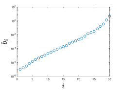
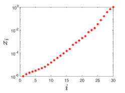
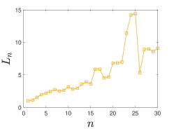
Figure 5.1: Opposite poles $\displaystyle b_{i}$ in the REIM (left); REIM interpolation points $\displaystyle x_{i}$ (mid); Lebesgue constant $\displaystyle L_{n}$ (right).

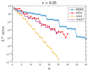
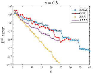
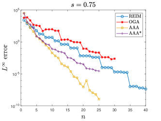
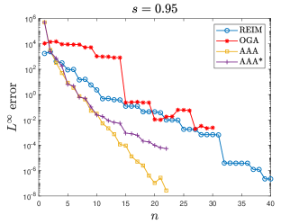
Figure 5.2: Maximum norm rational approximation errors for $\displaystyle x^{-s}$ on $\displaystyle[10^{-6},1]$.

5.1 Approximation of Power Functions

We start with a numerical comparison of the REIM, the OGA, and the popular AAA rational approximation algorithm for the target function $\displaystyle x^{-s}$ over $\displaystyle[10^{-6},1]$. Figure 5.1 shows the distribution of sorted poles $\displaystyle-b_{1},\ldots,-b_{30}$ and interpolation points $\displaystyle x_{1},\ldots,x_{30}$ used in the REIM. An interesting phenomenon is that the poles and interpolation points are both exponentially clustered at 0, consistent with the phenomenon observed in [46]. From Figure 5.1 (right), we observe that the Lebesgue constant $\displaystyle L_{n}$ of $\displaystyle\Pi_{n}$ grows slowly.

It is shown in Figure 5.2 that the AAA algorithm achieves the highest level of accuracy under the same number of iterations. However, the output of AAA is a barycentric representation of rational functions, which should be converted into the form $\displaystyle\sum_{i=1}^{n}\frac{c_{i}}{x+b_{i}}$ for our purpose (denoted by AAA*). Unfortunately, this process leads to significant loss of accuracy. It is also observed From Figure 5.2 that errors of AAA and AAA* do not decay after 22-25 iterations while the error of the REIM is finally smaller than AAA*.

5.2 Fractional Laplacian on Uniform Grids

On $\displaystyle\Omega=[-1,1]^{2}$ we consider the fractional Laplacian

$$(-\Delta)^{s}u=1$$ (5.1)

with $\displaystyle u=0$ on $\displaystyle\partial\Omega$. The reference exact solution is computed by

$$u\approx\sum_{j,k=1}^{j^{2}+k^{2}\leq 4\times 10^{6}}\lambda_{jk}^{-s}(1,u_{jk})u_{jk},$$

where $\displaystyle u_{jk}$ is the $\displaystyle L^{2}$ normalized eigenfunction of $\displaystyle-\Delta$ associated to the eigenvalue $\displaystyle\lambda_{jk}=(j^{2}+k^{2})\pi^{2}/4$. The fractional Laplacian is reduced by the REIM in Subsection 5.1 with $\displaystyle n=30$, $\displaystyle I=[10^{-6},1]$ to a series of integer-oder problems (3.5), which is further solved by finite difference on a uniform grid with mesh size $\displaystyle h_{i}=2^{-(i+3)},~{}i=1,...,5$. In this case, $\displaystyle\Lambda=10^{6}$ and $\displaystyle\eta=10^{-6}$ is enough to lower bound $\displaystyle\lambda_{\min}(\mathcal{A}_{h})/\Lambda$. The errors $\displaystyle e_{i}=\|u-u_{h_{i}}\|_{L^{2}(\Omega)}$ for different values of $\displaystyle s$ are recorded in Table 5.1 with order of convergence

$$\text{order}_{i+1}:=\log\left(\frac{e_{i+1}}{e_{i}}\right)\bigg{/}\log\left(\frac{h_{i+1}}{h_{i}}\right),\quad i=1,2,3,4.$$

In fact, convergence rates in Table 5.1 are consistent with the theoretical result $\displaystyle O(h^{\min\{2,2s+0.5\}})$ in [4].

$\displaystyle h_{i}$	$\displaystyle s=0.25$		$\displaystyle s=0.5$		$\displaystyle s=0.75$		$\displaystyle s=0.95$
	$\displaystyle L^{2}$ error	order	$\displaystyle L^{2}$ error	order	$\displaystyle L^{2}$ error	order	$\displaystyle L^{2}$ error	order
$\displaystyle 2^{-4}$	9.7461E-03	—	4.8415E-03	—	2.1959E-03	—	1.2359E-03	—
$\displaystyle 2^{-5}$	4.6362E-03	1.0719	1.6187E-03	1.5806	5.8485E-04	1.9087	3.1211E-04	1.9855
$\displaystyle 2^{-6}$	2.2817E-03	1.0229	5.4426E-04	1.5725	1.5303E-04	1.9342	7.8298E-05	1.995
$\displaystyle 2^{-7}$	1.0939E-03	1.0606	1.8480E-04	1.5583	3.9673E-05	1.9476	1.9599E-05	1.9982
$\displaystyle 2^{-8}$	4.7034E-04	1.2177	6.2553E-05	1.5628	1.0226E-05	1.9559	4.9019E-06	1.9993

Table 5.1: $\displaystyle L^{2}$ errors and convergence rates on uniform girds.

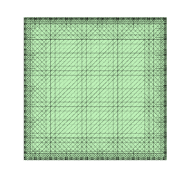
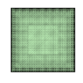
Figure 5.3: Graded grid $\displaystyle\mathcal{T}_{1}$ with 4225 vertices (left); graded grid $\displaystyle\mathcal{T}_{2}$ with 19585 vertices (right).

5.3 Fractional Laplacian on Graded Grids

On uniform grids, convergence rates of finite difference $\displaystyle L^{2}$ errors for fractional Laplacian are slower than $\displaystyle O(h^{2})$ when $\displaystyle s<0.75$, see Table 5.1. To improve the numerical accuracy, we test the performance of the EIM-based solver on graded grids appropriately resolving the boundary singularity. It is clear that adaptive mesh refinement is not applicable to rectangular meshes without introducing hanging nodes. Therefore, we discretize the fractional Laplacian (5.1) with $\displaystyle s=0.25$ by linear finite elements on locally refined triangular meshes. Let $\displaystyle\Omega$ be partitioned by the uniform mesh $\displaystyle\mathcal{T}_{0}$ with mesh size $\displaystyle h=0.25$ in each direction. Let $\displaystyle N(\mathcal{T})$ denote the number of vertices in $\displaystyle\mathcal{T}$ and $\displaystyle C_{T}$ the barycenter of a triangle $\displaystyle T$. For $\displaystyle j=1,2,3$, we set $\displaystyle\widetilde{\mathcal{T}}_{j}=\mathcal{T}_{j-1}$ successively mark and refine those triangles $\displaystyle T\in\widetilde{\mathcal{T}}_{j}$ satisfy

$${\rm area}(T)>\frac{6}{N(\widetilde{\mathcal{T}}_{j})}\log_{10}(N(\widetilde{\mathcal{T}}_{j})){\rm dist}(C_{T},\partial\Omega).$$

This loop terminates when $\displaystyle\widetilde{\mathcal{T}}_{j}$ fulfils $\displaystyle N(\widetilde{\mathcal{T}}_{j})\geq 4^{j}\times 10^{3}$ and we then set $\displaystyle\mathcal{T}_{j}=\widetilde{\mathcal{T}}_{j}$, see Figure 5.3 for $\displaystyle\mathcal{T}_{1}$ and $\displaystyle\mathcal{T}_{2}$.

Recall that $\displaystyle\mathbb{M}$ and $\displaystyle\mathbb{A}$ are linear finite element stiffness and mass matrices, respectively. The maximum eigenvalue $\displaystyle\lambda_{\max}(\mathcal{A}_{h})=\lambda_{\max}(\mathbb{M}^{-1}\mathbb{A})$ on highly contrast meshes grows faster than uniform mesh sequences. Thus we set the eigenvalue upper bound as $\displaystyle\Lambda=10^{8}$ and generate REIM rational approximants over $\displaystyle[10^{-8},1]$, see Figure 5.4 (left). In this case, $\displaystyle x^{-s}$ has greater singularity and more REIM iterations are needed to achieve the same accuracy as in Subsection 5.2. From Figure 5.4 (right), we observed that the FEM on graded grids $\displaystyle\{\mathcal{T}_{j}\}_{1\leq j\leq 4}$ is able to achieve higher-order convergence than the uniform-grid based FEM.

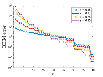
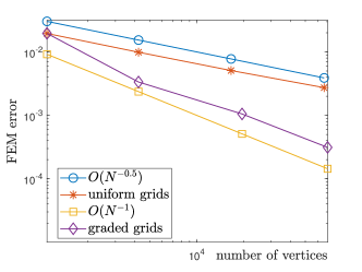
Figure 5.4: REIM $\displaystyle L^{\infty}$ error for $\displaystyle x^{-s}$ on $\displaystyle[10^{-8},1]$ (left); FEM $\displaystyle L^{2}$ errors for $\displaystyle s=0.25$, $\displaystyle N$ is the number of vertices (right).

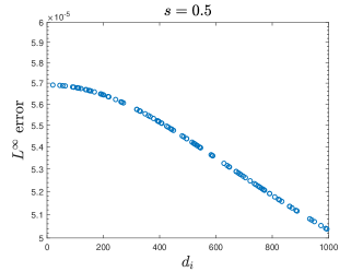
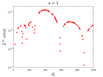
Figure 5.5: $\displaystyle L^{\infty}$ error of the REIM for $\displaystyle F_{0.5}$ (left) and $\displaystyle F_{1}$ (right).

5.4 Adaptive Step-Size Control for Fractional Heat Equations

On $\displaystyle\Omega=[0,1]^{2}$, we consider the fractional parabolic equation (3.7) with $\displaystyle\mathcal{A}=-\Delta$ and the exact solution

$$u(t,x,y)={\rm e}^{-t/20}\cos(2\pi t)\sin(\pi x)\sin(\pi y).$$ (5.2)

This problem with $\displaystyle s=0.5$ and $\displaystyle s=1$ is solved by the linear FEM on a uniform triangular mesh of mesh size $\displaystyle h=2^{-8}$. The upper bound of eigenvalues of $\displaystyle\mathcal{A}_{h}$ is again $\displaystyle\Lambda=10^{6}$ and $\displaystyle I=[10^{-6},1]$. Given the error tolerance $\displaystyle tol=10^{-4}$ and $\displaystyle\tau_{0}=10^{-3}$, we predict a new time step size of the implicit Euler method by the criterion (cf. [47])

$$\tau_{\text{new}}=0.8\tau_{m}\left(\frac{tol}{err_{m}}\right)^{1/2},$$ (5.3)

where $\displaystyle err_{m}$ is an error estimator described in Subsection 3.3. If $\displaystyle err_{m+1}\leq tol$, we accept $\displaystyle\tau_{m+1}=\tau_{\text{new}}$ and move forward to $\displaystyle t_{m+1}=t_{m}+\tau_{m+1}$; otherwise, a new $\displaystyle\tau_{\text{new}}$ is computed by (5.3) with $\displaystyle m$ replaced by $\displaystyle m+1$.

Recall that we need to approximate $\displaystyle\frac{1}{x^{s}+1/(\tau_{m}\Lambda^{s})}$ and $\displaystyle\frac{1}{x^{s}+\kappa_{1,m}/\Lambda^{s}}$ at each time step. To test the uniform accuracy of the REIM, we randomly select a point set $\displaystyle\mathcal{S}\subset[1,10^{3}]$ and consider the function set

$$F_{s}:=\{f_{i}\in C(I):f_{i}(x)=(x^{s}+d_{i}/\Lambda^{s})^{-1},~{}d_{i}\in\mathcal{S}\}.$$

The range $\displaystyle[1,10^{3}]$ contains all possible $\displaystyle 1/\tau_{m}$ and $\displaystyle\kappa_{1,m}$. Figure 5.5 shows the $\displaystyle L^{\infty}$ interpolation error of the REIM with $\displaystyle n=30$ for the functions in $\displaystyle F_{0.5}$ and $\displaystyle F_{1}$. The $\displaystyle L^{2}$ errors of numerical solutions and the accepted/rejected step sizes are presented in Figure 5.6. In the adaptive process, there are 243 steps and 5 rejected step sizes when $\displaystyle s=0.5$; 238 steps and 6 rejected step sizes when $\displaystyle s=1$.

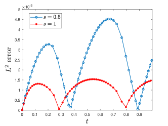
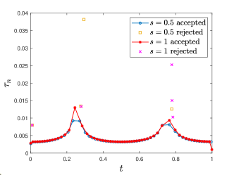
Figure 5.6: The $\displaystyle L^{2}$ error of numerical solutions (left); accepted steps and rejected step sizes (right).

5.5 Approximation of Other Functions

In the last experiment, we interpolate the functions in Subsections 3.4 and 3.5 using the REIM wit $\displaystyle n=30$. The left of Figure 5.7 shows the $\displaystyle L^{\infty}$ error of the REIM for $\displaystyle(x^{-\frac{1}{2}}+K_{i}x^{\frac{1}{2}})^{-1}$ on $\displaystyle[10^{-6},1]$, where the parameter $\displaystyle K_{i}$ was randomly selected from [$\displaystyle 10^{-6}$,1]. The right of Figure 5.7 shows the $\displaystyle L^{\infty}$ error of the REIM for $\displaystyle\exp(-\tau_{i}x)$ and $\displaystyle\varphi(-\tau_{i}x)$ on $\displaystyle[1,10^{6}]$, where the time step size $\displaystyle\tau_{i}$ was randomly selected from [$\displaystyle 0.002$,1].

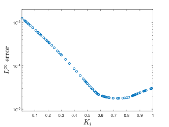
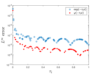
Figure 5.7: $\displaystyle L^{\infty}$ error for $\displaystyle(x^{-\frac{1}{2}}+K_{i}x^{\frac{1}{2}})^{-1}$ (left); $\displaystyle L^{\infty}$ error for $\displaystyle\exp(-\tau_{i}x)$ and $\displaystyle\varphi(-\tau_{i}x)$ (right).

References

- [1] C. Bucur, E. Valdinoci, Nonlocal diffusion and applications, Vol. 20 of Lecture Notes of the Unione Matematica Italiana, Springer, [Cham]; Unione Matematica Italiana, Bologna, 2016. doi:10.1007/978-3-319-28739-3.
- [2] A. Lischke, G. Pang, M. Gulian, et al., What is the fractional Laplacian? A comparative review with new results, J. Comput. Phys. 404 (2020) 109009, 62. doi:10.1016/j.jcp.2019.109009.
- [3] M. D’Elia, Q. Du, C. Glusa, M. Gunzburger, X. Tian, Z. Zhou, Numerical methods for nonlocal and fractional models, Acta Numer. 29 (2020) 1–124. doi:10.1017/s096249292000001x.
- [4] A. Bonito, J. E. Pasciak, Numerical approximation of fractional powers of elliptic operators, Math. Comp. 84 (295) (2015) 2083–2110. doi:10.1090/S0025-5718-2015-02937-8.
- [5] P. N. Vabishchevich, Numerically solving an equation for fractional powers of elliptic operators, J. Comput. Phys. 282 (2015) 289–302. doi:10.1016/j.jcp.2014.11.022.
- [6] S. Harizanov, R. Lazarov, S. Margenov, P. Marinov, Y. Vutov, Optimal solvers for linear systems with fractional powers of sparse SPD matrices, Numer. Linear Algebra Appl. 25 (5) (2018) e2167, 24. doi:10.1002/nla.2167.
- [7] C. Hofreither, A unified view of some numerical methods for fractional diffusion, Comput. Math. Appl. 80 (2) (2020) 332–350. doi:10.1016/j.camwa.2019.07.025.
- [8] T. Danczul, J. Schöberl, A reduced basis method for fractional diffusion operators I, Numer. Math. 151 (2) (2022) 369–404. doi:10.1007/s00211-022-01287-y.
- [9] K. E. Holter, M. Kuchta, K.-A. Mardal, Robust preconditioning for coupled Stokes-Darcy problems with the Darcy problem in primal form, Comput. Math. Appl. 91 (2021) 53–66. doi:10.1016/j.camwa.2020.08.021.
- [10] A. Budiša, X. Hu, M. Kuchta, K.-A. Mardal, L. Zikatanov, Rational approximation preconditioners for multiphysics problems, in: In: Georgiev, I., Datcheva, M., Georgiev, K., Nikolov, G. (eds) Numerical Methods and Applications. NMA 2022. Lecture Notes in Computer Science, vol 13858. Springer, Cham., Springer, 2023. doi:10.1007/978-3-031-32412-3_9.
- [11] L. Lopez, V. Simoncini, Analysis of projection methods for rational function approximation to the matrix exponential, SIAM J. Numer. Anal. 44 (2) (2006) 613–635. doi:10.1137/05062590.
- [12] V. Druskin, L. Knizhnerman, M. Zaslavsky, Solution of large scale evolutionary problems using rational Krylov subspaces with optimized shifts, SIAM J. Sci. Comput. 31 (5) (2009) 3760–3780. doi:10.1137/080742403.
- [13] P. P. Petrushev, V. A. Popov, Rational approximation of real functions, Vol. 28 of Encyclopedia of Mathematics and its Applications, Cambridge University Press, Cambridge, 1987.
- [14] Y. Nakatsukasa, O. Sète, L. N. Trefethen, The AAA algorithm for rational approximation, SIAM J. Sci. Comput. 40 (3) (2018) A1494–A1522. doi:10.1137/16M1106122.
- [15] C. Hofreither, An algorithm for best rational approximation based on barycentric rational interpolation, Numer. Algorithms 88 (1) (2021) 365–388. doi:10.1007/s11075-020-01042-0.
- [16] Y. Li, L. Zikatanov, C. Zuo, A reduced conjugate gradient basis method for fractional diffusion, SIAM J. Sci. Comput. (2024) S68–S87doi:10.1137/23M1575913.
- [17] M. Barrault, Y. Maday, N. C. Nguyen, A. T. Patera, An ‘empirical interpolation’ method: application to efficient reduced-basis discretization of partial differential equations, C. R. Math. Acad. Sci. Paris 339 (9) (2004) 667–672. doi:10.1016/j.crma.2004.08.006.
- [18] Y. Maday, N. C. Nguyen, A. T. Patera, G. S. H. Pau, A general multipurpose interpolation procedure: the magic points, Commun. Pure Appl. Anal. 8 (1) (2009) 383–404. doi:10.3934/cpaa.2009.8.383.
- [19] S. Chaturantabut, D. C. Sorensen, Nonlinear model reduction via discrete empirical interpolation, SIAM J. Sci. Comput. 32 (5) (2010) 2737–2764. doi:10.1137/090766498.
- [20] J. L. Eftang, M. A. Grepl, A. T. Patera, E. M. Rönquist, Approximation of parametric derivatives by the empirical interpolation method, Found. Comput. Math. 13 (5) (2013) 763–787. doi:10.1007/s10208-012-9125-9.
- [21] Y. Maday, O. Mula, A generalized empirical interpolation method: application of reduced basis techniques to data assimilation, in: Analysis and numerics of partial differential equations, Vol. 4 of Springer INdAM Ser., Springer, Milan, 2013, pp. 221–235. doi:10.1007/978-88-470-2592-9\_13.
- [22] F. Negri, A. Manzoni, D. Amsallem, Efficient model reduction of parametrized systems by matrix discrete empirical interpolation, J. Comput. Phys. 303 (2015) 431–454. doi:10.1016/j.jcp.2015.09.046.
- [23] N. C. Nguyen, J. Peraire, Efficient and accurate nonlinear model reduction via first-order empirical interpolation, J. Comput. Phys. 494 (2023) Paper No. 112512, 19. doi:10.1016/j.jcp.2023.112512.
- [24] Y. Li, A new analysis of empirical interpolation methods and Chebyshev greedy algorithms, arXiv:2401.13985 (2024).
- [25] G. G. Lorentz, M. v. Golitschek, Y. Makovoz, Constructive approximation, Vol. 304 of Grundlehren der mathematischen Wissenschaften [Fundamental Principles of Mathematical Sciences], Springer-Verlag, Berlin, 1996, advanced problems. doi:10.1007/978-3-642-60932-9.
- [26] J. W. Siegel, J. Xu, Sharp bounds on the approximation rates, metric entropy, and n-widths of shallow neural networks, Found. Comput. Math. (2022). doi:10.1007/s10208-022-09595-3.
- [27] A. Cohen, R. DeVore, G. Petrova, P. Wojtaszczyk, Optimal stable nonlinear approximation, Found. Comput. Math. 22 (3) (2022) 607–648. doi:10.1007/s10208-021-09494-z.
- [28] T. Danczul, C. Hofreither, J. Schöberl, A unified rational krylov method for elliptic and parabolic fractional diffusion problems, Numer Linear Algebra Appl. 30 (2) (2023) e2488. doi:10.1002/nla.2488.
- [29] A. R. Barron, A. Cohen, W. Dahmen, R. A. DeVore, Approximation and learning by greedy algorithms, Ann. Statist. 36 (1) (2008) 64–94. doi:10.1214/009053607000000631.
- [30] R. A. DeVore, G. G. Lorentz, Constructive approximation, Vol. 303 of Grundlehren der mathematischen Wissenschaften [Fundamental Principles of Mathematical Sciences], Springer-Verlag, Berlin, 1993.
- [31] Y. Maday, O. Mula, G. Turinici, Convergence analysis of the generalized empirical interpolation method, SIAM J. Numer. Anal. 54 (3) (2016) 1713–1731. doi:10.1137/140978843.
- [32] Y. Li, J. W. Siegel, Entropy-based convergence rates for greedy algorithms, Math. Models Methods Appl. Sci. 34 (5) (2024) 779–802. doi:10.1142/S0218202524500143.
- [33] R. A. DeVore, V. N. Temlyakov, Some remarks on greedy algorithms, Adv. Comput. Math. 5 (2-3) (1996) 173–187. doi:10.1007/BF02124742.
- [34] V. Temlyakov, Multivariate approximation, Vol. 32 of Cambridge Monographs on Applied and Computational Mathematics, Cambridge University Press, Cambridge, 2018. doi:10.1017/9781108689687.
- [35] S. Harizanov, R. Lazarov, S. Margenov, P. Marinov, J. Pasciak, Comparison analysis of two numerical methods for fractional diffusion problems based on the best rational approximations of on , in: Advanced finite element methods with applications, Vol. 128 of Lect. Notes Comput. Sci. Eng., Springer, Cham, 2019, pp. 165–185. doi:10.1007/978-3-030-14244-5\_9.
- [36] A. Jannelli, R. Fazio, Adaptive stiff solvers at low accuracy and complexity, J. Comput. Appl. Math. 191 (2) (2006) 246–258. doi:10.1016/j.cam.2005.06.041.
- [37] W. M. Boon, M. Hornkjø l, M. Kuchta, K.-A. Mardal, R. Ruiz-Baier, Parameter-robust methods for the Biot-Stokes interfacial coupling without Lagrange multipliers, J. Comput. Phys. 467 (2022) Paper No. 111464, 25. doi:10.1016/j.jcp.2022.111464.
- [38] S. Harizanov, I. Lirkov, S. Margenov, Rational approximations in robust preconditioning of multiphysics problems, Mathematics 10 (5) (2022) 780.
- [39] M. Hochbruck, A. Ostermann, Exponential integrators, Acta Numer. 19 (2010) 209–286. doi:10.1017/S0962492910000048.
- [40] Y.-W. Li, X. Wu, Exponential integrators preserving first integrals or Lyapunov functions for conservative or dissipative systems, SIAM J. Sci. Comput. 38 (3) (2016) A1876–A1895. doi:10.1137/15M1023257.
- [41] M. Hochbruck, C. Lubich, On Krylov subspace approximations to the matrix exponential operator, SIAM J. Numer. Anal. 34 (5) (1997) 1911–1925. doi:10.1137/S0036142995280572.
- [42] N. J. Higham, Functions of matrices, Society for Industrial and Applied Mathematics (SIAM), Philadelphia, PA, 2008, theory and computation. doi:10.1137/1.9780898717778.
-
[43]
F. Hirsch, Intégrales de résolvantes et calcul symbolique, Ann. Inst. Fourier (Grenoble) 22 (4) (1972) 239–264.
doi:10.5802/aif.439.
URL https://doi.org/10.5802/aif.439 - [44] J. H. Schwarz, The generalized Stieltjes transform and its inverse, J. Math. Phys. 46 (1) (2005) 013501, 8. doi:10.1063/1.1825077.
- [45] B. Carl, Entropy numbers, -numbers, and eigenvalue problems, J. Functional Analysis 41 (3) (1981) 290–306. doi:10.1016/0022-1236(81)90076-8.
- [46] L. N. Trefethen, Y. Nakatsukasa, J. A. C. Weideman, Exponential node clustering at singularities for rational approximation, quadrature, and PDEs, Numer. Math. 147 (1) (2021) 227–254. doi:10.1007/s00211-020-01168-2.
- [47] E. Hairer, S. P. Nörsett, G. Wanner, Solving ordinary differential equations. I, Vol. 8 of Springer Series in Computational Mathematics, Springer-Verlag, Berlin, 1987, nonstiff problems. doi:10.1007/978-3-662-12607-3.