Non-spinning tops are stable

Abstract

We consider coupled gravitational and electromagnetic perturbations of a family of five-dimensional Einstein-Maxwell solutions that describes both magnetized black strings and horizonless topological stars. We find that the odd perturbations of this background lead to a master equation with five Fuchsian singularities and compute its quasinormal mode spectrum using three independent methods: Leaver, WKB and numerical integration. Our analysis confirms that odd perturbations always decay in time, while spherically symmetric even perturbations may exhibit for certain ranges of the magnetic fluxes instabilities of Gregory-Laflamme type for black strings and of Gross-Perry-Yaffe type for topological stars. This constitutes evidence that topological stars and black strings are classically stable in a finite domain of their parameter space.

1 Introduction

The physics of black holes is responsible for some of the deepest puzzles in our quest to formulate a unified quantum theory of gravity. On one hand, black holes have an entropy proportional to the area of the event horizon in Planck units, and hence, according to Statistical Mechanics, an enormous number of states ($e^{10^{90}}$ for the Sgr.A black hole at the center of the Milky Way). On the other hand, uniqueness theorems indicate that General Relativity is not able to distinguish any of these states and this, in turn, leads to violations of quantum unitarity. It is also possible to argue Mathur:2009hf ; Almheiri:2012rt ; Guo:2021blh that the only way to avoid such violations is if these states give different physics from that of the classical General-Relativity black-hole solution at the scale of the event horizon.

However, constructing such states is no easy feat: as the black-hole horizon is null, any horizon-sized object we can construct using normal four-dimensional matter will immediately fall in. The only mechanism to avoid gravitational collapse in a classical theory is to use (or mimic) higher-dimensional theories with nontrivial fluxes wrapping topologically-nontrivial cycles Gibbons:2013tqa ; deLange:2015gca , of the type one naturally finds in String Theory.

Furthermore, the black hole horizon is perhaps the only thing in our universe that grows when gravity becomes stronger. Hence, if one wants to construct horizon-sized extreme-compact-objects (ECO’s) that replace the black hole, these objects must contain non-perturbative solitonic degrees of freedom, which become lighter and larger when gravity becomes stronger.

For supersymmetric and extremal-non-supersymmetric black holes there is an almost-20-year history of string-theory and supergravity constructions of such horizon-sized ECO’s, which are also known as microstate geometries, fuzzballs geometries, or “topological stars" Bena:2013dka . The string-theory ingredients that enter their construction have exactly the properties needed to avoid collapse and grow when gravity becomes stronger. However, constructing and analyzing topological stars for non-supersymmetric black holes is much more challenging, requiring in general solving non-linear PDE’s that, absent supersymmetry, do not factorize.

Besides some artisanal solutions Jejjala:2005yu ; Bena:2009qv , there are now three systematic routes to build such solutions. The oldest is the floating-JMaRT factorization Bossard:2014ola ; Bossard:2014yta , which can in principle produce non-extremal rotating solutions, but which unfortunately does not seem to produce solutions that have the same charges and angular momenta as non-extremal black holes with a macroscopic horizon Bena:2015drs ; Bena:2016dbw ; Bossard:2017vii . The second is to use numerics in a consistent truncation to three-dimensional supergravity Mayerson:2020tcl to produce microstrata Ganchev:2021pgs ; Ganchev:2021ewa ; Ganchev:2023sth ; Houppe:2024hyj that have the same charges as non-extremal asymtptotically-AdS rotating black holes. The third is to use the Bah-Heidmann factorization Bah:2020pdz to produce non-extremal non-rotating multi-bubble topological stars, which can have both flat-space and AdS asymptotics Bah:2020ogh ; Bah:2021owp ; Bah:2021rki ; Bah:2021irr ; Heidmann:2021cms ; Bah:2022pdn ; Bah:2022yji ; Bah:2023ows . Absence of rotation notwithstanding, this later method appears to be the most prolific at generating solitonic solutions with non-extremal black-hole charges and mass, including Schwarzschild microstate Bah:2022yji ; Bah:2023ows .

The main question about these non-extremal microstate geometries is whether they are stable or unstable, and what are the physical implications of their stability or absence thereof. Since the asymptotically-AdS₃ solutions are dual to coherent CFT states that have both right movers and left movers, one can argue that generic solutions with a large number of identical CFT strands should be unstable Chowdhury:2008bd , much like the JMaRT solution is Cardoso:2005gj ; Chowdhury:2007jx ; Bianchi:2023rlt . However, this argument does not extend to solutions without an AdS near-horizon region, such as Schwarzschild microstates.

The purpose of this paper is to investigate the stability under coupled gravitational and electromagnetic perturbations of the simplest spherically-symmetric topological star, which can be constructed as four-dimensional Euclidean Schwarzschild (ES) solution times time, to which one adds magnetic flux on the ES bolt. The solution is specified by two parameters $r_{s}$ and $r_{b}$ that interpolate between a magnetic black string solution with a finite-area event horizon when $r_{s}>r_{b}$ and a smooth horizonless solution one when $r_{s}<r_{b}$. Throughout this paper we will call the former the black string and the later the top star. The top star solution is one of the key ingredients in the building of the more general multi-bubble Bah-Heidmann solutions, and hence our investigation is the first step in a programme to determine the stability or instability of these solutions and the physical consequences thereof.

The equations governing the perturbation around the black string and top star are the same, and couple the electromagnetic fluctuations to the gravitational ones. They separate into a rather intractable parity-even sector and a more tractable parity-odd sector, on which we focus in this paper. We find that in this sector the perturbations separate into two coupled systems of ODE’s. We show that one of these systems boils down to two independent second-order ODE’s for the so-called master variables. These ODE’s have five Fuchsian singularities, and cannot be mapped to a Heun equation or confluent version thereof. Hence, they are harder to solve then the scalar perturbations of black holes Regge:1957td ; Teukolsky:1973ha , of D-brane bound states Bianchi:2021mft ; Bianchi:2021mft , and of topological stars Bianchi:2023sfs ; Heidmann:2023ojf ; Cipriani:2024ygw , where the linear dynamics is described by confluent forms of the Heun equation.

We primarily rely on the Leaver method to find the quasinormal (QNM) frequencies of topological stars and magnetic black strings. The then verify the results against those obtained through direct numerical integration and WKB analysis. The WKB approximation works well when the orbital number of the perturbation is large. Direct numerical integration of the differential equation produces reliable results for frequencies with a small imaginary part. Our calculations show that QNM frequencies of odd perturbations have always negative imaginary part, so they represent modes decaying in time.

For even perturbations, we are able to separate the equations only for spherically symmetric perturbations and find stable solutions for all topological stars with $r_{s}<2r_{b}$ and black strings with $r_{b}<2r_{s}$ in agreement with Bah:2021irr ; Stotyn:2011tv . Our analysis provide a unifying picture that interpolates between the Gross-Perry-Yaffe-type instability of top stars with zero or small magnetic fields Gross:1982cv ; Witten:1981gj ; Bah:2021irr ; Stotyn:2011tv and the Gregory-Laflamme instability Gregory:1993vy ; Gregory:1994bj of magnetized black strings with zero or small magnetic charge Miyamoto:2007mh . Both these instabilities manifest themselves through the existence of QNMs that blow up in time.

The key result of our calculation is that in the regimes of parameters where these instabilities are absent, all other perturbations decay in time. Hence, in these regimes, both the top star and the magnetized black strings are stable!

In Section 2 we derive the system of ordinary differential equations governing the odd sector of the coupled gravitational and electromagnetic perturbations. In Section 3 we compute the spectrum of QNM frequencies for odd perturbations. In Section 4 we determine the regimes of Gregory-Laflamme instability. Finally, in Section 5 we present some conclusions and future directions.

Note added: When this work was nearly complete, we were informed that another group was working independently on the same problem Paolo-new . Although there is significant overlap between our results, our analysis and that of Paolo-new also focus on different aspects and numerical methods and are therefore complementary to each other. We have compared some of our numerical results to those of Paolo-new , finding very good agreement.

2 Gravitational and electromagnetic perturbations

We consider solutions of Einstein-Maxwell theory in five dimensions describing magnetically-charged topological stars and black strings. Our goal is to study linear perturbations of the metric and gauge field around these backgrounds. The study of perturbations around magnetically charged backgrounds poses a technical problem well known in the literature on black-hole perturbation theory Gerlach:1980tx ; Kodama:2003kk ; Pereniguez:2023wxf : the usual decoupling between even and odd perturbations does not occur. Here we circumvent this problem by dualizing the vector field into a two-form potential $C_{\mu\nu}$ with field strength $F_{\mu\nu\rho}=3\partial_{[\mu}C_{\nu\rho]}$. In terms of this field, the equations of motion are

$$R_{\mu\nu}-\frac{1}{2}g_{\mu\nu}R = \frac{1}{4}\left(F_{\mu\alpha\beta}F_{\nu}{}^{\alpha\beta}-\frac{1}{6}g_{\mu\nu}F_{\alpha\beta\gamma}F^{\alpha\beta\gamma}\right)\,,$$ (2.1)

$$\nabla_{\mu}F^{\mu\nu\rho} = 0\,.$$ (2.2)

We study linear perturbations around solutions of (2.1) and (2.2) with metric ${\bar{g}}_{\mu\nu}$ and two-form potential ${\bar{C}}_{\mu\nu}$ given by Horowitz:1991cd ; Bah:2020ogh ; Bah:2020pdz

$$\mathrm{d}{\bar{s}}^{2} = -f_{s}(r)\mathrm{d}t^{2}+\frac{\mathrm{d}r^{2}}{f_{s}(r)f_{b}(r)}+r^{2}\left(\mathrm{d}\theta^{2}+\sin\theta^{2}\mathrm{d}\phi^{2}\right)+f_{b}(r)\mathrm{d}y^{2}\,,$$ (2.3)

$${\bar{C}} = \frac{\sqrt{3r_{s}r_{b}}}{r}\,\mathrm{d}t\wedge\mathrm{d}y\,,$$ (2.4)

where $r_{s}$, $r_{b}$ are some real positive numbers and

$$f_{s}(r)=1-\frac{r_{s}}{r}\,,\hskip 28.45274ptf_{b}(r)=1-\frac{r_{b}}{r}\,.$$ (2.5)

There are two regimes of interest:

$${\rm Black\leavevmode\nobreak\ string}: \qquad r_{b}<r_{s}$$

$${\rm Topological\leavevmode\nobreak\ star}: \qquad r_{s}<r_{b}$$ (2.6)

The first is called the black string regime Horowitz:1991cd , in which the solution has an event horizon at $r=r_{s}$. In the second, the solution describes a topological star Bah:2020ogh ; Bah:2020pdz , which is a smooth horizonless solution provided the coordinate $y$ is periodically identified with period

$$y\sim y+\frac{4\pi r_{b}^{3/2}}{\sqrt{r_{b}-r_{s}}}\,.$$ (2.7)

For this periodicity the spacetime smoothly ends at the hypersurface $r=r_{b}$. The geometry near $r=r_{b}$ is ${\mathbb{R}}_{t}\times{\mathbb{R}}^{2}\times{\mathbb{S}}^{2}$.

2.1 Linear perturbations

We consider perturbations of the background metric and two-form potentials,

$$g_{\mu\nu}={\bar{g}}_{\mu\nu}+h_{\mu\nu}\,,\hskip 28.45274ptC_{\mu\nu}={\bar{C}}_{\mu\nu}+c_{\mu\nu}\,.$$ (2.8)

Following Regge:1957td , we separate the perturbations according to their transformations under parity in even- and odd-types. For the background solutions we are considering, even and odd perturbations do not couple. Therefore, we can study them separately. Here we focus on odd perturbations, which are considerably simpler. These are given by

$$h_{\mu\nu}\mathrm{d}x^{\mu}\mathrm{d}x^{\nu}\, = \,2\,e^{-{\rm i}\omega t}\sum_{a=t,r,y}h_{a}(r)\mathrm{d}x^{a}\left[-\frac{1}{\sin\theta}\frac{\partial Y_{\ell m}}{\partial\phi}\mathrm{d}\theta+\sin\theta\frac{\partial Y_{\ell m}}{\partial\theta}\mathrm{d}\phi\right]\,,$$ (2.9)

$$c_{\mu\nu}\mathrm{d}x^{\mu}\wedge\mathrm{d}x^{\nu}\, = \,2\,e^{-{\rm i}\omega t}\sum_{a=t,r,y}c_{a}(r)\mathrm{d}x^{a}\wedge\left[-\frac{1}{\sin\theta}\frac{\partial Y_{\ell m}}{\partial\phi}\mathrm{d}\theta+\sin\theta\frac{\partial Y_{\ell m}}{\partial\theta}\mathrm{d}\phi\right]\,,$$ (2.10)

where $Y_{\ell m}(\theta,\phi)$ are the spherical harmonics satisfying

$$\left[\frac{1}{\sin\theta}\frac{\partial}{\partial\theta}\left(\sin\theta\frac{\partial}{\partial\theta}\right)+\frac{1}{\sin^{2}\theta}\frac{\partial^{2}}{\partial\phi^{2}}+\ell(\ell+1)\right]Y_{\ell m}=0\,.$$ (2.11)

Since the background is spherically symmetric there is no dependence on $m$, so from now on we set $m=0$. In addition, we consider no dependence on the coordinate $y$ for the time being. Plugging (2.9) and (2.10) into the field equations, (2.1) and (2.2), and expanding to linear order in the perturbations, one finds two decoupled systems of ordinary differential equations: one for the $(h_{t},h_{r},c_{y})$ perturbations

$$h_{r}^{\prime}(r)+\left[\frac{r(r_{s}+r_{b})-2r_{s}r_{b}}{r(r-r_{s})(r-r_{b})}\right]h_{r}(r)+\frac{ir^{3}\omega h_{t}(r)}{\left(r-r_{b}\right)\left(r-r_{s}\right){}^{2}}=0\,,$$

$$h_{t}^{\prime}(r)-\frac{2h_{t}(r)}{r}+{\rm i}\left[\frac{\omega^{2}r^{3}{-}\left(\ell{+}2\right)\left(\ell{-}1\right)\left(r{-}r_{s}\right)}{\omega r^{3}}\right]h_{r}(r)+\frac{\sqrt{3r_{b}r_{s}}c_{y}(r)}{r(r-r_{b})}=0\,,$$ (2.12)

$$c_{y}^{\prime\prime}(r){+}\frac{r_{s}c_{y}^{\prime}(r)}{r\left(r{-}r_{s}\right)}{+}\left[\frac{\left(r^{5}\omega^{2}-\ell(\ell{+}1)r^{2}\left(r{-}r_{s}\right){+}3r_{b}r_{s}\left(r_{s}{-}r\right)\right)}{r^{2}\left(r{-}r_{b}\right)\left(r{-}r_{s}\right){}^{2}}\right]c_{y}(r)$$

$$\qquad\qquad\qquad\qquad\qquad\qquad{+}\frac{i\sqrt{3}(\ell+2)\left(\ell-1\right)\sqrt{r_{b}r_{s}}h_{r}(r)}{r^{4}\omega}=0\,,$$

and one for $(c_{t},c_{r},h_{y})$ perturbations

$$c_{r}^{\prime}(r)+\left[\frac{r\left(r_{b}+r_{s}\right)-2r_{b}r_{s}}{r\left(r-r_{b}\right)\left(r-r_{s}\right)}\right]c_{r}(r)+\frac{ir^{3}\omega c_{t}(r)}{\left(r-r_{b}\right)\left(r-r_{s}\right){}^{2}}=0\,,$$

$$c_{t}^{\prime}(r)+\frac{\left[\ell(\ell+1)(r-r_{s})-r^{3}\omega^{2}\right]c_{r}(r)}{ir^{3}\omega}-\frac{\sqrt{3}\ell(\ell+1)\sqrt{r_{b}r_{s}}h_{y}(r)}{r\left(r-r_{b}\right)}=0\,,$$ (2.13)

$$h_{y}^{\prime\prime}(r){+}\frac{r_{s}h_{y}^{\prime}(r)}{r(r{-}r_{s})}{+}\left[\frac{\left(r^{5}\omega^{2}{-}\left(r{-}r_{s}\right)\left(r\left(\ell(\ell{+}1)r{-}2r_{b}\right){+}3r_{b}r_{s}\right)\right)}{r^{2}\left(r{-}r_{b}\right)\left(r{-}r_{s}\right){}^{2}}\right]h_{y}(r){-}\frac{i\sqrt{3}c_{r}(r)\sqrt{r_{b}r_{s}}}{r^{4}\omega}=0\,.$$

Before studying the complete system, we discuss two limits of interest.

2.2 Schwarzschild black string and soliton limits

The limits are the $r_{b}\to 0$ and the $r_{s}\to 0$ limits. In the first the background solution corresponds to the “Schwarzschild black string” (meaning a four-dimensional Schwarzschild solution times a transverse direction). The second limit corresponds to a horizonless solution which we are going to call the Schwarzschild soliton. These solutions are mapped one into another via a double Wick rotation along the coordinates $t$ and $y$ and an exchange of $r_{s}\leftrightarrow r_{b}$. This does not imply, as we are going to see, that the equations for the perturbations around these backgrounds coincide (up to an exchange of $r_{s}\leftrightarrow r_{b}$). The reason is that here we are considering perturbations with no dependence in $y$. Therefore, the perturbations are not mapped one into each other by the double Wick rotation, even if the background solutions are.

• Schwarzschild black string: $r_{b}\to 0$. In this limit the full system reduces to four independent second-order differential equations for $h_{r},h_{y},c_{r},c_{y}$. When recast into Schrödinger form, they are given by

  $$\Psi_{s}^{\prime\prime}(r)+Q_{s}(r)\Psi_{s}(r)=0\,,$$ (2.14)

  where $Q_{s}$ is the spin-$s$ Regge-Wheeler potential Regge:1957td

  $$Q_{s}(r)=\frac{r^{4}\omega^{2}-\ell(\ell+1)r(r-r_{s})+s^{2}r_{s}\left(r-r_{s}\right)+\frac{r_{s}^{2}}{4}}{r^{2}(r-r_{s})^{2}}\,,$$ (2.15)

  and

  $$\Psi_{s}\sim\left\{\begin{array}[]{ccc}c_{r}&\nobreak\leavevmode\nobreak\leavevmode\nobreak\leavevmode\nobreak\leavevmode\hfil&s=0\\ h_{y},c_{y}&&s=1\\ h_{r}&&s=2\end{array}\right.\,.$$ (2.16)

• Schwarzschild soliton: $r_{s}\to 0$. The four differential equations can be cast in Schrödinger form,

  $$\Psi_{\epsilon}^{\prime\prime}+Q_{\epsilon}(r)\Psi_{\epsilon}=0\,,$$ (2.17)

  with

  $$Q_{\epsilon}=\frac{r^{3}\omega^{2}-\ell(\ell+1)r+2\epsilon r_{b}}{r^{2}\left(r-r_{b}\right)}\,,$$ (2.18)

  and

  $$\Psi_{s}\sim\left\{\begin{array}[]{ccc}c_{r},c_{y}&\nobreak\leavevmode\nobreak\leavevmode\nobreak\leavevmode\nobreak\leavevmode\hfil&\epsilon=0\\ h_{r},h_{y}&&\epsilon=1\\ \end{array}\right.\,.$$ (2.19)

2.2.1 The $(h_{r},c_{y},h_{t})$ system

We focus on the system (2.1) describing the perturbations $(h_{t},h_{r},c_{y})$. The first equation can be solved for $h_{t}$, leading to a coupled system of two differential equations for $h_{r}$, $c_{y}$. The system can be decoupled by the linear transformation,

$$h_{r}= g_{h}(r)\left[\Psi_{+}(r)+\Psi_{-}(r)\right]\,,$$ (2.20)

$$c_{y}= g_{c}(r)\left[(1+\gamma)\Psi_{+}(r)+(1-\gamma)\Psi_{-}(r)\right]\,,$$

with

$$g_{h}(r)={r^{7\over 2}\over(r-r_{b})(r-r_{s})^{3/2}}\,,\hskip 28.45274ptg_{c}(r)=-{{\rm i}(2r_{b}+3r_{s})\over 2\omega\sqrt{3r_{b}r_{s}}}{r^{1\over 2}\over(r-r_{s})^{1\over 2}}\,,$$ (2.21)

and

$$\gamma\equiv\sqrt{1+\frac{12(\ell+2)(\ell-1)r_{b}r_{s}}{(2r_{b}+3r_{s})^{2}}}\,.$$ (2.22)

In terms of these variables the system reduces to two decoupled ordinary differential equations of the Schrödinger form,

$$\Psi^{\prime\prime}_{\pm}+Q_{\pm}\Psi_{\pm}=0\,,$$ (2.23)

with

$$Q_{\pm}\,= \frac{r^{3}}{\left(r-r_{s}\right)^{2}\left(r-r_{b}\right)}\left[\omega^{2}-\frac{\ell(\ell+1)}{r^{2}}+\frac{\left(2r_{b}+3r_{s}\right)\left(1\pm\gamma\right)+2r_{s}\left(\ell^{2}+\ell+1\right)}{2r^{3}}\right.$$ (2.24)

$$\left.-\frac{r_{s}\left[\left(2r_{b}+3r_{s}\right)\left(1\pm\gamma\right)+8r_{b}+\frac{3}{2}r_{s}\right]}{2r^{4}}+\frac{15r_{b}r_{s}^{2}}{4r^{5}}\right]\,.$$

Let us remark that (2.23) is a differential equation with five Fuchsian singularities: three regular ones at $r=0,r_{s},r_{b}$, and two colliding at $r=\infty$. Crucially, this radial equation cannot be mapped to a Heun equation or any of its confluent versions, as is the case for the scalar perturbations in the topological star geometry, which are described by a Confluent Heun equation Bianchi:2023sfs , similar to all black holes in the Kerr-Newman family Bianchi:2022wku .

2.2.2 The $(h_{y},c_{t},c_{r})$ system

We can proceed analogously for the system (2.13). We solve the first equation for $c_{t}$, which yields a system of two coupled second-order ODEs. Then we look for a change of variables of the form

$$\begin{bmatrix}h_{y}\\ c_{r}\\ \end{bmatrix}=\begin{bmatrix}g_{1+}(r)&g_{1-}(r)\\ g_{2+}(r)&g_{2-}(r)\\ \end{bmatrix}\begin{bmatrix}\Phi_{+}\\ \Phi_{-}\\ \end{bmatrix}\,,$$ (2.25)

and fix the functions $g_{1+},g_{2-},g_{2+}$ and $g_{2-}$ such that the system decouples in two independent second-order ODEs for $\Phi_{+}$ and $\Phi_{-}$. We find that for this system this not possible. However, for the choice of functions

$$g_{1+}=g_{2+}=1\,,\hskip 28.45274ptg_{1-}=-g_{2-}=\frac{r^{3}}{\left(r-r_{b}\right)\left(r-r_{s}\right)}\,,$$ (2.26)

we find that the second system (2.13) reduces to the following differential equations

$$\Phi^{\prime\prime}_{\pm}+\frac{r_{s}}{r\left(r-r_{s}\right)}\Phi^{\prime}_{\pm}+\frac{[-4r_{b}r_{s}+r\left(2r_{b}+r_{s}\right)]\omega\pm{\rm{i}}\sqrt{3r_{b}r_{s}}\,r\left[1+\ell\left(\ell+1\right)\omega^{2}\right]}{2r^{2}\left(r-r_{b}\right)\left(r-r_{s}\right)}\Phi_{\mp}$$ (2.27)

$$+\left[\frac{r^{3}\omega^{2}}{\left(r-r_{b}\right)\left(r-r_{s}\right)^{2}}\pm\frac{{\rm{i}}\sqrt{3r_{b}r_{s}}\,}{2r\left(r-r_{b}\right)\left(r-r_{s}\right)}\left(\ell(\ell+1)\,\omega+\frac{1}{\omega}\right)\right.$$

$$\left.+\frac{2r\left(r_{b}-\ell(1+\ell)r\right)-r_{s}\left(r+2r_{b}\right)}{2r^{2}\left(r-r_{b}\right)\left(r-r_{s}\right)}\right]\Phi_{\pm}=0\,.$$

Then we can use the equation which does not contain derivatives of $\Phi_{-}$ (equivalently, $\Phi_{+}$) and solve it (for $\Phi_{-}$). After plugging the resulting expression in the remaining equation, we get a fourth-order ODE for $\Phi_{+}$. Given its complexity, we omit the details and the study of the QNMs.

3 QNMs of topological stars and black strings

In this section we compute the QNM spectrum associated to the $(h_{t},h_{r},c_{y})$ perturbations, whose dynamics is described by the master equations (2.23). We will mainly use a semi-analytical method developed by Leaver Leaver:1985ax , which has been recently applied to the study of scalar perturbations of topological stars, Bianchi:2023sfs ; Heidmann:2023ojf ; Cipriani:2024ygw . Nevertheless, we will compare the results obtained using Leaver’s method against those obtained using the WKB approximation and via a direct numerical integration of the differential equation.

QNMs correspond to solutions of the Schrodinger-type equation (2.23) satisfying the boundary conditions

$$\Psi(r)\underset{r\to r_{0}}{\sim}(r-r_{0})^{\lambda_{0}}\,,\hskip 28.45274pt\Psi(r)\underset{r\to\infty}{\sim}r^{\lambda_{\infty}}e^{i\omega r}\,.$$ (3.1)

with

$$r_{0}=\left\{\begin{array}[]{ccc}r_{b}&\nobreak\leavevmode\nobreak\leavevmode\nobreak\leavevmode\nobreak\leavevmode\nobreak\leavevmode\hfil&{\rm(top\leavevmode\nobreak\ star)}\\ r_{s}&&{\rm(black\leavevmode\nobreak\ string)}\\ \end{array}\right.\,,\hskip 56.9055pt\lambda_{0}\in\left\{\begin{array}[]{ccc}\mathbb{R}_{+}&\nobreak\leavevmode\nobreak\leavevmode\nobreak\leavevmode\nobreak\leavevmode\nobreak\leavevmode\hfil&{\rm(top\leavevmode\nobreak\ star)}\\ {\rm i}\,\mathbb{R}_{-}&&{\rm(black\leavevmode\nobreak\ string)}\\ \end{array}\right.\,.$$ (3.2)

Namely, we are imposing outgoing boundary conditions at infinity for both background solutions. The difference lies in the boundary conditions imposed at $r_{0}$. For top stars we just demand regularity at the cap: $r=r_{b}$. Instead, for the black string we impose incoming boundary conditions at the horizon: $r=r_{s}$. The specific values of $\lambda_{0}$ and $\lambda_{\infty}$ can be obtained by solving the differential equation around $r=r_{0}$ and $r=\infty$. The details are given in sections 3.3 and 3.4.

Solutions satisfying these boundary conditions exist only for a discrete choice of complex frequencies $\omega_{n}$: the QNMs. The rest of the section is organized as follows. First, in sections 3.1 and 3.2 we briefly describe the WKB approximation and the numerical integration methods we are going to use to further confirm the results obtained using Leaver’s method. The latter will be discussed in sections 3.3 (top star) and 3.4 (black string).

3.1 WKB approximation

A rough estimate of the QNM frequencies, $\omega$, can be obtained from a WKB semiclassical approximation of the wave solution Schutz:1985km ; Cardoso:2008bp ; Bianchi:2020des ; Bianchi:2020yzr ; Bianchi:2021mft around the “light rings”: extrema of the effective potential $-Q(r)$ where both $Q$ and its first derivative vanish:

$$Q(r_{c};\omega_{c})=Q^{\prime}(r_{c};\omega_{c})=0\,.$$ (3.3)

To estimate the QNM frequencies, we promote $\omega_{c}$ to a complex number (adding a small imaginary part) and demand that the integral between two zeros $r_{\pm}$ of $Q(r)$ satisfies the Bohr-Sommerfeld quantization condition:

$$\int_{r_{-}}^{r_{+}}\sqrt{Q(r;\omega)}dr=\pi\left(n+\frac{1}{2}\right)\,.$$ (3.4)

The solution to linear order in the imaginary part of $\omega$ is given by the WKB formula, namely

$$\omega_{n}^{\rm WKB}=\omega_{c}-{\rm i}\left(n+\frac{1}{2}\right)\frac{\sqrt{\partial_{r}^{2}Q}}{\partial_{\omega}Q}\Big{|}_{\omega=\omega_{c},r=r_{c}}\,.$$ (3.5)

3.2 Direct numerical integration

QNM frequencies can be alternatively obtained via a direct numerical integration of the differential equation in the domain $r\in[r_{0},\infty]$ with boundary conditions (3.1). Since both $r=r_{0}$ and $r=\infty$ are singular points, boundary conditions cannot be imposed exactly at these points, but one can choose some arbitrary points nearby. The procedure has several steps: First, one determines the solution (with the appropriate boundary conditions) as a Taylor expansion around $r_{0}$. Then, one evaluates the solution at a point $r_{0}+\epsilon$ with $\epsilon$ small, and uses the result as a boundary condition to find a numerical solution, $\Psi_{0}$. One then proceeds in the same way to compute a numerical solution $\Psi_{\infty}$ satisfying outgoing boundary conditions at infinity.

The QNM frequencies are then obtained by requiring the matching of the two functions at an intermediate point. This is equivalent to demanding the vanishing of the Wronskian:

$$\Psi_{0}^{\prime}(r;\omega)\Psi_{\infty}(r;\omega)-\Psi_{0}(r;\omega)\Psi_{\infty}^{\prime}(r;\omega)=0\,,$$ (3.6)

at some point $r$ in the middle. We notice that the Wronskian is independent of the choice of this point. Thus, (3.6) becomes an equation for $\omega$ whose solutions are the QNMs. When comparing this method against the Leaver method, we will bear in mind that this numerical method is known to be numerically stable only for frequencies with a small imaginary part ae16f484-8e04-30db-a6a3-902e6f6fd388 ; Berti:2009wx ; Cardoso:2014sna ; Bianchi:2023sfs .

3.3 QNMs: top stars

In this section we compute the QNM spectrum of top stars using Leaver’s method. As explained in the previous section, top stars correspond to smooth horizonless geometries ending a cap at $r=r_{b}$ with $r_{b}>r_{s}$. Hence, QNMs in this geometry correspond to solutions of (2.23) satisfying regular boundary conditions at the cap and behaving as an outgoing wave at infinity. Given this, we consider the following ansatz

$$\Psi(r)=e^{i\omega r}r^{-{3\over 2}}(r-r_{s})^{\lambda_{s}}\sum_{n=0}^{\infty}c_{n}\left(\frac{r-r_{b}}{r-r_{s}}\right)^{n}\,,$$ (3.7)

with

$$\lambda_{s}=\frac{1}{2}+{{\rm i}\omega\over 2}(r_{b}+2r_{s})\,.$$ (3.8)

The expansion (3.7) satisfies the required boundary conditions at the cap and infinity, and solves (2.23) near $r=r_{b}$ and near $r\to\infty$. Plugging (3.7) into (2.23) yields a four-term recursion relation,

$$\alpha_{n}c_{n+1}+\beta_{n}c_{n}+\gamma_{n}c_{n-1}+\delta_{n}c_{n-2}=0\,,\hskip 14.22636pt\quad n\geq 0\,.$$ (3.9)

The explicit expressions of the coefficients $\alpha_{n},\beta_{n},\gamma_{n}$ and $\delta_{n}$ for $\Psi_{+}$ are

$$\alpha_{n}\,= -(n+1)(n+2)\,,$$ (3.10)

$$\beta_{n}\,= \ell(\ell{+}1){+}2n(n{+}2){+}1{-}\gamma+\frac{r_{s}(3(1+\gamma)-2n(n-2))}{2r_{b}}{-}3{\rm i}(n{+}1)\omega r_{b}{-}\frac{\omega^{2}r_{b}^{3}}{r_{b}{-}r_{s}}\,,$$

$$\gamma_{n}\,= {-}n(n{+}1){+}1{+}\gamma{+}\frac{r_{s}(3\gamma{-}4(n{-}3)n{-}2\ell(\ell{+}1){-}5)}{2r_{b}}+\frac{1}{2}i\omega\left(2nr_{b}{+}r_{b}{+}(10n{-}7)r_{s}\right){+}\frac{\omega^{2}r_{b}^{2}\left(r_{b}{+}7r_{s}\right)}{4\left(r_{b}{-}r_{s}\right)}\,,$$

$$\delta_{n}\,= \frac{(n-2)r_{s}\left(n-2i\omega r_{s}-2\right)}{r_{b}}-\frac{1}{4}\omega r_{s}\left(\omega r_{b}+4i(n-2)+4\omega r_{s}\right)-\frac{\omega^{2}r_{s}^{3}}{r_{b}-r_{s}}\,.$$

The coefficients of the recursion for $\Psi_{-}$ are obtained by sending $\gamma\to-\gamma$.

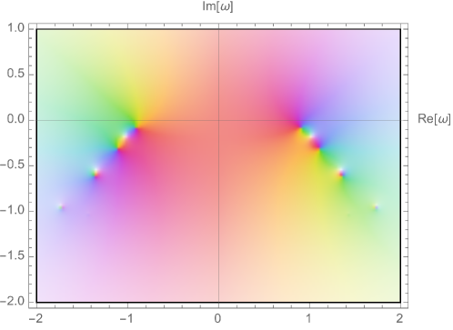
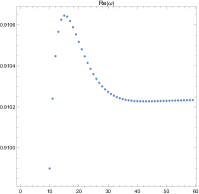
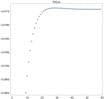
Figure 1: Left Panel) QNMs for top star with $r_{b}=1$, $r_{s}=0.8$ and $\ell=2$. Right Panels) Convergence of the continuous-fraction method.

$\ell$	Leaver($n=0$)	Dir. Int.
$2$	$0.9102-0.0774i$	$0.9102-0.0774i$
$3$	$1.3939-0.0477i$	$1.3939-0.0477i$
$4$	$1.8618-0.0286i$	$1.8618-0.0286i$
$5$	$2.3241-0.0164i$	$2.3241-0.0164i$
$8$	$3.6952-0.0019i$	$3.6952-0.0019i$
$10$	$4.6003-0.0003i$	$4.6003-0.0003i$

$n$	Leaver ($\ell=2$)
$0$	$0.9102-0.0774i$
$1$	$1.1201-0.3126i$
$2$	$1.3775-0.6018i$
$3$	$1.6711-0.9105i$
$4$	$1.9868-1.2224i$
$5$	$2.3415-1.5428i$

Table 1: QNMs for top star with $r_{b}=1$, $r_{s}=0.8$.

Truncating $n$ to some large number $N$, the recursion relation (3.9) becomes an $N$-dimensional matrix equation $M\cdot c=0$, where $c$ is a vector containing the $c_{n}$ coefficients entering in the ansatz (3.7). Therefore, a non-trivial solution exists only if the determinant of $M$ vanishes, which provides the equation satisfied by the QNM frequencies. However, we are not going to use the vanishing of the determinant to find the QNMs. Instead, we find more convenient to first tridiagonalize $M$,

$$\alpha^{\prime}_{0}\,= \alpha_{0},\quad\beta^{\prime}_{0}=\beta_{0}\,,$$

$$\alpha^{\prime}_{1}\,= \alpha_{1},\quad\beta^{\prime}_{1}=\beta_{1},\quad\gamma^{\prime}_{1}=\gamma_{1}$$

$$\alpha^{\prime}_{n}\,= \alpha_{n},\quad\beta^{\prime}_{n}=\beta_{n}-\frac{\delta_{n}}{\gamma^{\prime}_{n-1}}\alpha^{\prime}_{n},\quad\gamma^{\prime}_{n}\,=\, \gamma_{n}-\frac{\delta_{n}}{\gamma^{\prime}_{n-1}}\beta^{\prime}_{n},\quad\delta^{\prime}_{n}=0\,,\quad n\geq 2$$

and then use the fact that the integrability of the three-term recursion boils down to the continuous fraction equation:

$$\beta^{\prime}_{n}+\frac{\alpha^{\prime}_{n}\gamma^{\prime}_{n}}{\beta^{\prime}_{n-1}-\frac{\alpha^{\prime}_{n-2}\gamma^{\prime}_{n-1}}{\beta^{\prime}_{n-2}-\dots}}+\frac{\alpha^{\prime}_{n}\gamma^{\prime}_{n+1}}{\beta^{\prime}_{n+1}-\frac{\alpha^{\prime}_{n+1}\gamma^{\prime}_{n+2}}{\beta^{\prime}_{n+2}-\dots}}=0\,.$$ (3.11)

The QNM frequencies can be obtained by solving the above equation for a particular $n$, let us say $n=0$. In practice, the continuous fraction is truncated by keeping $N$ terms, with $N$ a large enough number. In Figure 1 (left) the result for the QNM frequencies is displayed for the $\ell=2$ mode in a top star with $r_{s}=0.8$, $r_{b}=1$ with $N=50$. The plots on the right show the convergence of the method, which typically occurs for $N\geq 30$.

In Table 1 we display the results for QNM frequencies for the fundamental mode $n=0$ as $\ell$ varies from 2 to 10. The results are compared against those obtained from a direct numerical integration of the differential equation, showing an excellent agreement. We omit the results based on a WKB approximation of the solution as the latter fails in reproducing the imaginary part of the QNM frequencies for the low $n$ modes.

Finally, in appendix A we collect more results for various representative choices of $r_{s}$, $r_{b}$, $\ell$. In all the solutions we have checked, QNM frequencies have negative imaginary parts, suggesting the stability of top stars against metric and electromagnetic odd perturbations.

3.4 QNM: black string

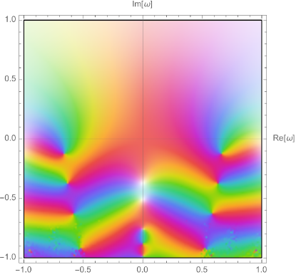
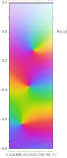
Figure 2: $R_{+}$ QNM’s for black string with $r_{b}=0.8$, $r_{s}=1$, $\ell=2$

$\ell$	WKB	Leaver	Dir. Int.
$2$	$0.6323-0.1239i$	$0.6648-0.1225i$	$0.6648-0.1225i$
$3$	$1.0608-0.1267i$	$1.0826-0.1263i$	$1.083-0.1263i$
$4$	$1.4678-0.1282i$	$1.4839-0.1279i$	$1.4839-0.1279i$
$5$	$1.8659-0.129i$	$1.8787-0.1288i$	$1.8787-0.1288i$
$8$	$3.0402-0.1301i$	$3.0482-0.13i$	$3.0482-0.13i$
$10$	$3.8166-0.1304i$	$3.8229-0.1303i$	$3.8229-0.1303i$

Table 2: The fundamental $n=0$ QNM for a black string with $r_{b}=0.8$, $r_{s}=1$,

.

The analysis for the black string $r_{b}<r_{s}$ follows mutatis mutandis the same steps than that for topological stars, but now incoming boundary conditions have to be imposed at the horizon $r=r_{s}$. Therefore, the ansatz now becomes

$$\Psi(r)=e^{i\omega r}r^{-{3\over 2}}(r-r_{s})^{\lambda_{s}}(r-r_{b})^{\lambda_{b}}\sum_{n=0}^{\infty}c_{n}\left(\frac{r-r_{s}}{r-r_{b}}\right)^{n}\,,$$ (3.12)

with

$$\lambda_{s}={1\over 2}+{\omega r_{s}^{3\over 2}\over\sqrt{r_{b}-r_{s}}}\,,\hskip 28.45274pt\lambda_{b}=1+{{\rm i}\omega\over 2(r_{s}-r_{b})}\left(2r_{s}^{2}-r_{b}^{2}-r_{b}r_{s}+2\sqrt{r_{s}^{3}(r_{s}-r_{b})}\right)\,.$$ (3.13)

Plugging this into (2.23) yields again a four-term recursion relation as in (3.9), but this time with coefficients given by:

$$\alpha_{n} =-(n+1)^{2}r_{s}+\frac{2i(n+1)\omega r_{s}^{2}}{\sigma}\,,$$

$$\beta_{n} =-\frac{1}{2}r_{s}\left(-2\gamma\sigma^{2}+5\gamma-2\ell^{2}-2\ell+2n^{2}\sigma^{2}-6n^{2}-6n\sigma^{2}+2n+2\sigma^{2}+1\right)$$

$$-\frac{i(\sigma+1)\omega\left(2n\sigma^{2}-6n\sigma+12n+\sigma^{2}+5\sigma-2\right)r_{s}^{2}}{2\sigma}-\frac{(\sigma+1)^{3}\omega^{2}r_{s}^{3}}{\sigma^{2}}\,,$$

$$\gamma_{n} =\frac{1}{2}r_{s}\left(-2\gamma\sigma^{2}+5\gamma+2\ell^{2}\sigma^{2}-2\ell^{2}+2\ell\sigma^{2}-2\ell+4n^{2}\sigma^{2}-6n^{2}-16n\sigma^{2}+16n+14\sigma^{2}-9\right)\,$$

$$-\frac{i(\sigma+1)^{2}\omega\left(n\sigma^{3}-2n\sigma^{2}+6n\sigma-6n-2\sigma^{3}+4\sigma^{2}-10\sigma+8\right)r_{s}^{2}}{\sigma}+\frac{\left(\sigma^{2}-8\sigma+8\right)(\sigma+1)^{4}\omega^{2}r_{s}^{3}}{4\sigma^{2}}\,,$$

$$\delta_{n} =-\frac{i(2n-5)(\sigma-2)(\sigma-1)(\sigma+1)^{3}\omega r_{s}^{2}}{2\sigma}-(n-3)(n-2)(\sigma-1)(\sigma+1)r_{s}$$

$$+\frac{(\sigma-2)^{2}(\sigma-1)(\sigma+1)^{5}\omega^{2}r_{s}^{3}}{4\sigma^{2}}\,,$$

with

$$\sigma=\sqrt{1-{r_{b}\over r_{s}}}\,.$$ (3.14)

Figure 2 shows some QNM frequencies (different overtones) $r_{s}=1$, $r_{b}=0.8$ and $\ell=2$, again for the $\Psi_{+}$ perturbation. Those for $n=0$ with $\ell$ varying from $2$ to $10$ are displayed in Table 2, together with a comparison against the WKB and direct integration methods. As we can see, we find an pretty good agreement. Finally, other representative examples are collected in the Appendix A. For $r_{b}=0$ we reproduce the results for Schwarzschild black holes, as expected.

As in the analysis of the topological star, we find that for all choices of $r_{s}$, $r_{b}$, $\ell$ we have checked the imaginary parts of the QNM frequencies of black strings are always negative, strongly suggesting the stability of these solutions against this type of perturbations.

4 Gregory-Laflamme instabilities

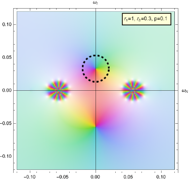
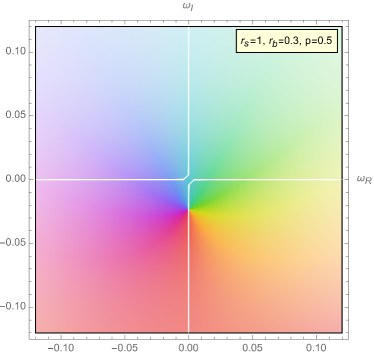
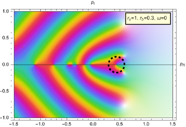
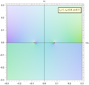
Figure 3: Black string unstable modes for various parameters; the frequency of the unstable mode is at $\omega=0.0332837i$ (Top left), $p=0.435943$ (Bottom left).

Black strings and branes in dimensions higher than four typically exhibit a classical instability, known as the Gregory-Laflamme (GL) instability Gregory:1994bj . A characteristic feature of the GL perturbations is that they have a momentum, $p$, along the internal directions. Typically, the instability appears when $p$ is smaller than a certain threshold value, $p_{\star}$, while the system is stable under perturbations with $p>p_{\star}$. This suggests that the mode with $p=p_{\star}$ (which is referred to as the threshold unstable mode) is time independent.

Based on the existence of a threshold time-independent mode, the domain of GL stability of black strings was determined in Miyamoto:2007mh to be $r_{s}<2r_{b}$. Furthermore, Bah:2021irr ; Stotyn:2011tv used the double Wick rotation symmetry that exchanges black strings with topological stars, $r_{s}\leftrightarrow r_{b}$ and $\omega\leftrightarrow{\rm i}p$ to argue that top stars are stable when $r_{b}<2r_{s}$. We also know that when $r_{b}$ is fixed and $r_{s}=0$, the top star becomes Euclidean Schwarzschild times time, and this solution suffers from a Gross-Perry-Yaffe instability Gross:1982cv ; Witten:1981gj . Hence, we expect the instability of top stars with $0<r_{s}<r_{b}/2$ to be of the same type Bah:2021irr ; Stotyn:2011tv .

Here we review the arguments of Miyamoto:2007mh ; Bah:2021irr , adapting them to the more general perturbations where both $p$ and $\omega$ are non-vanishing. We then apply the Leaver method to compute the QNM frequencies and show directly the existence of modes with positive imaginary parts outside of the stability domains.

Let us consider the following even perturbation of the metric and two-form with $\ell=0$ (hence, spherically-symmetric),

$$h_{\mu\nu}\mathrm{d}{x}^{\mu}\mathrm{d}{x}^{\nu}\,= e^{{\rm i}py-{\rm i}\omega t}\left[h_{1}(r)\mathrm{d}r^{2}{+}r^{2}k(r)\left(\mathrm{d}\theta^{2}{+}\sin^{2}\theta\,\mathrm{d}\phi^{2}\right){+}2\,h_{2}(r)\,\mathrm{d}r\,\mathrm{d}y{+}2\,h_{3}(r)\,\mathrm{d}r\,\mathrm{d}t\right]\,,$$ (4.1)

$$c_{\mu\nu}\mathrm{d}{x}^{\mu}\mathrm{d}{x}^{\nu}\,= 2e^{{\rm i}py-{\rm i}\omega t}c(r)\,\mathrm{d}t\wedge\mathrm{d}y\,.$$

One can check that for any choice of $p$ and $\omega$ this is not pure gauge: $h_{\mu\nu}$ cannot be written as $\nabla_{(\mu}\zeta_{\nu)}$. The field equations (2.1) and (2.2) allow us to solve for $c$, $h_{1}$, $h_{2}$ and $h_{3}$ in terms of $k$, and we find that the latter satisfies the second-order differential equation

$${d\over dr}\left[A(r)k^{\prime}(r)\right]-B(r)k(r)=0\,,$$ (4.2)

with

$$A(r) =\frac{\left(r{-}r_{b}\right)\left(r{-}r_{s}\right)}{{\cal W}(r)^{2}}\,,$$ (4.3)

$$B(r) =\frac{r^{3}{\cal W}(r)\left[p^{2}\left(r{-}r_{s}\right){-}\omega^{2}\left(r{-}r_{b}\right)\right]+2\left(r{-}r_{b}\right)\left(r{-}r_{s}\right)\left[p^{2}\left(2r_{b}{-}r_{s}\right){-}\omega^{2}\left(2r_{s}{-}r_{b}\right)\right]}{{\cal W}(r)^{3}\left(r{-}r_{b}\right)\left(r{-}r_{s}\right)}\,,$$

and

$${\cal W}(r)=p^{2}\left(4r-3r_{s}\right)-\omega^{2}\left(4r-3r_{b}\right)\,.$$ (4.4)

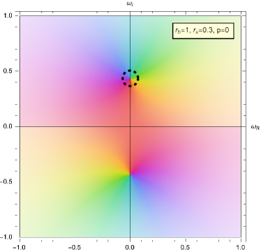
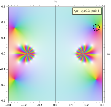
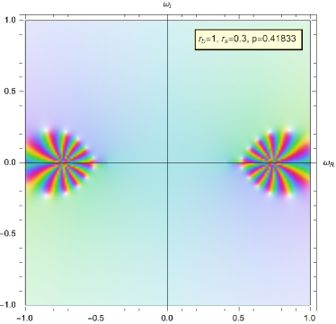
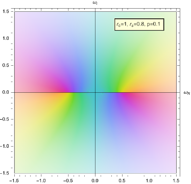
Figure 4: GL unstable modes for the topological star for various parameters: the frequencies are $\omega=0.435929i$ (top left) and $\omega=0.260928-0.166396i$ (top right).

We look for solutions to (4.2) satisfying the boundary conditions,

$$k(r)\underset{r\to r_{0}}{\sim}(r-r_{0})^{\lambda_{0}}\,,\hskip 56.9055ptk(r)\underset{r\to\infty}{\sim}e^{{\rm i}r\sqrt{\omega^{2}-p^{2}}}\,,$$ (4.5)

where $r_{0}={\rm{max}}\left[r_{s},r_{b}\right]$ and $\lambda_{0}$ is determined by solving the equation near $r=r_{0}$ and imposing incoming (for the black string) or regular (for the top star) boundary conditions at $r=r_{0}$. The GL modes correspond to solutions of (4.2) satisfying (4.5), and exhibiting an exponential decay at infinity Gregory:1994bj :

$${\rm Re}\left({\rm i}\sqrt{\omega^{2}-p^{2}}\right)<0\,.$$ (4.6)

In order to review the arguments presented in Miyamoto:2007mh ; Bah:2021irr in a unified way, let us first consider perturbations where $p$ is real and $\omega$ is purely imaginary and (4.6) is automatically satisfied. Multiplying (4.2) by $k(r)$, integrating it over the domain $[r_{0},\infty]$, and integrating by parts, we obtain:

$$\int^{\infty}_{r_{0}}\mathrm{d}r\left[A(r)\left(k^{\prime}(r)\right)^{2}+B(r)k(r)^{2}\right]=\int^{\infty}_{r_{0}}d\left[A(r)k(r)k^{\prime}(r)\right]=0\,.$$ (4.7)

The vanishing of the right hand side follows from the fact that $A(r)$ vanishes at $r_{0}$ and $k(r)$ vanishes at infinity. In addition if $p$ is real and $\omega$ purely imaginary, both $A(r)$ and $B(r)$ are real and positive in the domain:

$${\rm{top\leavevmode\nobreak\ star:}}\,\,\,r_{s}<r_{b}<2r_{s}\,,\hskip 28.45274pt{\rm{black\leavevmode\nobreak\ string:}}\,\,\,r_{b}<r_{s}<2r_{b}\,.$$ (4.8)

Thus, the only (real) solution of (4.7) is the trivial one, $k=0$. The geometry is therefore stable in this domain.

Given this, we provide further evidence applying again Leaver’s method. Since the procedure is analogous to the one described in the previous section, we shall ignore the technical details and present directly the results in Figures 3 and 4, where we plot the argument of the QNM eigenvalue equation for various choices of $r_{s}$ and $r_{b}$. The QNM frequencies show up as peaks on these plots.

A summary of our findings is:

• Black string (Figure 3): We find unstable modes only in the regime $r_{s}>2r_{b}$ for $p<p_{\star}\approx 0.435943$ in agreement with expectations in Miyamoto:2007mh .

• Top star (Figure 4): We find unstable modes for $r_{b}>2r_{s}$ and $p$ small enough. However when $p$ is finite, it cannot be arbitrarily small since regularity of the geometry requires the quantization condition:

  $$p=\frac{n_{y}}{R_{y}}=n_{y}\,\frac{{\sqrt{r_{b}-r_{s}}}}{2r_{b}^{3/2}}\,,\hskip 28.45274ptn_{y}\in{\mathbb{Z}}\,,$$ (4.9)

  We find that all modes with $n_{y}\geq 1$ are stable, therefore only the $n_{y}=0$ mode leads to a potential instability.

5 Conclusions

We have calculated the QNM frequencies associated to odd perturbations of topological stars and magnetized black strings in five-dimensional Einstein-Maxwell theory. Our analysis of the QNM spectrum mainly relies on Leaver’s method Leaver:1985ax , which has been suitably generalized in order to apply it to an ODE with five Fuchsian singularities, reducing the 4-term recursion relation to a 3-term one via a tri-diagonalization of the eigenvalue matrix.

We have confirmed the expectations of Bah:2021irr ; Stotyn:2011tv which suggest classical stability inside the domain

$${\rm{top\leavevmode\nobreak\ star:}}\,\,\,r_{s}<r_{b}<2r_{s}\,,\hskip 28.45274pt{\rm{black\leavevmode\nobreak\ string:}}\,\,\,r_{b}<r_{s}<2r_{b}\,,$$ (5.1)

as we have found that all the perturbations we have considered inside the above domains decay exponentially in time. Outside of these domains we have verified that topological stars suffer from a Gross-Perry-Yaffe-type instability Gross:1982cv , whereas magnetic black strings suffer from the usual Gregory-Laflamme instability Miyamoto:2007mh . Such instabilities reflect themselves on the existence of QNMs with positive imaginary part which are associated to even perturbations with $\ell=0$.

There are several obvious next steps to our investigation. The first is to study the possible gravitational-wave signatures that may distinguish top stars from black holes: multipolar structureMayerson:2020tpn ; Bianchi:2020des , echoes Ikeda:2021uvc and tidal effects during the inspiral phase of black-hole merger Fucito:2023afe .

The next is to consider the even perturbations, and try to solve the underlying system of ODE’s numerically. This will involve a shooting problem in several functions of one variable. Systems of similar complexity have been solved by shooting in other circumstances Ganchev:2021pgs ; Buchel:2000ch , so we believe this problem is within reach.

Another extension of our calculation is to the running-Bolt solutions Bena:2009qv , which are also obtained by magnetizing the bolt of Euclidean Schwarzschild times time in five dimensions. For these solutions we also expect a Gross-Perry-Yaffe-type instability for small magnetic fluxes, and possibly a stable solution for larger fluxes Avery . Another cohomogeneity-one solution with fluxes that can be studied using our method is the magnetized Atiyah-Hitchin solution Atiyah:1985dv ; Bena:2007ju , which is the M-theory uplift of Type-IIA Orientifold 6-planes with fluxes.

Our calculation serves as a first step towards and a benchmark in the determination of the stability or lack thereof for more generic non-extremal topological stars that have a fluxed bolt. The most generic such solutions are cohomogeneity-two Bah:2021owp , and hence determining the quasinormal frequencies will require solving PDE’s, using methods similar to those of Dias:2009iu ; Dias:2014eua ; Santos:2015iua . These calculations should reduce in certain limits to the calculations we do here, and hence our calculations should serve as a useful benchmark for these more complicated calculations.

Appendix A QNMs

In this appendix we collect some tables displaying QNM frequencies corresponding to the perturbations $\Psi_{+}$ (left) and $\Psi_{-}$ (right) for various choices of $r_{s}$, $r_{b}$ and $\ell$.

• $r_{s}=0.8$, $r_{b}=1$:

  $\ell$	Leaver ($n=0$)	Dir. Int. ($n=0$)
  $2$	$0.9102-0.0774i$	$0.9102-0.0774i$
  $3$	$1.3939-0.0477i$	$1.3939-0.0477i$
  $4$	$1.8618-0.0286i$	$1.8618-0.0286i$
  $5$	$2.3241-0.0164i$	$2.3241-0.0164i$
  $6$	$2.7833-0.0087i$	$2.7833-0.0087i$
  $7$	$3.2403-0.0043i$	$3.2403-0.0043i$
  $8$	$3.6952-0.0019i$	$3.6952-0.0019i$
  $9$	$4.1484-0.0008i$	$4.1484-0.0008i$
  $10$	$4.6003-0.0003i$	$4.6003-0.0003i$

  $\ell$	Leaver ($n=0$)	Dir. Int ($n=0$)
  $2$	$1.5803-0.1064i$	$1.5803-0.1064i$
  $3$	$2.0518-0.0694i$	$2.0518-0.0694i$
  $4$	$2.5181-0.0454i$	$2.5181-0.0454i$
  $5$	$2.9815-0.0288i$	$2.9815-0.0288i$
  $6$	$3.4429-0.0174i$	$3.4429-0.0174i$
  $7$	$3.9025-0.0098i$	$3.9025-0.0098i$
  $8$	$4.3604-0.0051i$	$4.3604-0.0051i$
  $9$	$4.8166-0.0024i$	$4.8166-0.0024i$
  $10$	$5.2711-0.001i$	$5.2711-0.001i$

  $n$	Leaver ($\ell=2$)
  $0$	$0.9102-0.0774i$
  $1$	$1.1201-0.3126i$
  $2$	$1.3775-0.6018i$
  $3$	$1.6711-0.9105i$
  $4$	$1.9868-1.2224i$
  $5$	$2.3415-1.5428i$

  $n$	Leaver ($\ell=2$)
  $0$	$1.5803-0.1064i$
  $1$	$1.7748-0.345i$
  $2$	$2.0085-0.6302i$
  $3$	$2.274-0.9405i$
  $4$	$2.5645-1.2634i$
  $5$	$2.8598-1.5919i$

  $n$	Leaver ($\ell=10$)	Dir. Int. ($\ell=10$)
  $0$	$4.6003-0.0003i$	$4.6003-0.0003i$
  $1$	$4.7872-0.0321i$	$4.7872-0.0321i$
  $2$	$4.9538-0.1546i$	$4.9538-0.1546i$
  $3$	$5.139-0.3201i$	$-$
  $4$	$5.3355-0.5135i$	$-$
  $5$	$5.5417-0.729i$	$-$

  $n$	Leaver ($\ell=10$)	Dir. Int. ($\ell=10$)
  $0$	$5.2711-0.001i$	$5.2711-0.001i$
  $1$	$5.4367-0.0486i$	$5.4368-0.0486i$
  $2$	$5.5997-0.1799i$	$-$
  $3$	$5.7793-0.348i$	$-$
  $4$	$5.9699-0.5423i$	$-$
  $5$	$6.1702-0.7575i$	$-$

• $r_{s}=0$, $r_{b}=1$:

  $\ell$	Leaver ($n=0$)
  $2$	$1.8517-1.2691i$
  $3$	$3.0513-1.3549i$
  $4$	$4.157-1.3815i$
  $5$	$5.222-1.3933i$
  $6$	$6.266-1.3996i$
  $7$	$7.2979-1.4034i$
  $8$	$8.3221-1.4059i$
  $9$	$9.3411-1.4076i$
  $10$	$10.3564-1.4088i$

  $\ell$	Leaver ($n=0$)
  $2$	$2.2995-1.4362i$
  $3$	$3.3569-1.425i$
  $4$	$4.3888-1.4206i$
  $5$	$5.409-1.4185i$
  $6$	$6.423-1.4173i$
  $7$	$7.4333-1.4165i$
  $8$	$8.4412-1.416i$
  $9$	$9.4474-1.4156i$
  $10$	$10.4524-1.4154i$

  $n$	Leaver ($\ell=2$)
  $0$	$1.8517-1.2691i$
  $1$	$1.4597-2.7725i$
  $2$	$1.0743-4.6179i$
  $3$	$0.8437-6.6137i$
  $4$	$0.7107-8.6372i$
  $5$	$0.6269-10.6623i$

  $n$	Leaver ($\ell=2$)
  $0$	$2.2995-1.4362i$
  $1$	$1.9111-3.0645i$
  $2$	$1.5047-4.9713i$
  $3$	$1.2273-7.0143i$
  $4$	$1.0492-9.0811i$
  $5$	$0.927-11.1432i$

  $n$	Leaver ($\ell=10$)
  $0$	$10.3564-1.4088i$
  $1$	$10.2491-2.828i$
  $2$	$10.0721-4.2681i$
  $3$	$9.8284-5.7402i$
  $4$	$9.5235-7.2556i$
  $5$	$9.1654-8.8256i$

  $n$	Leaver ($\ell=10$)
  $0$	$10.4524-1.4154i$
  $1$	$10.3457-2.841i$
  $2$	$10.1698-4.2876i$
  $3$	$9.9277-5.766i$
  $4$	$9.6249-7.2876i$
  $5$	$9.2694-8.8632i$

• $r_{b}=0.8$, $r_{s}=1$:

  $\ell$	WKB ($n=0$)	Leaver ($n=0$)	Dir. Int. ($n=0$)
  $2$	$0.6323-0.1239i$	$0.6648-0.1225i$	$0.6648-0.1225i$
  $3$	$1.0608-0.1267i$	$1.0826-0.1263i$	$1.083-0.1263i$
  $4$	$1.4678-0.1282i$	$1.4839-0.1279i$	$1.4839-0.1279i$
  $5$	$1.8659-0.129i$	$1.8787-0.1288i$	$1.8787-0.1288i$
  $6$	$2.2595-0.1295i$	$2.2702-0.1294i$	$2.2702-0.1294i$
  $7$	$2.6507-0.1299i$	$2.6598-0.1297i$	$2.6598-0.1297i$
  $8$	$3.0402-0.1301i$	$3.0482-0.13i$	$3.0482-0.13i$
  $9$	$3.4288-0.1303i$	$3.4358-0.1302i$	$3.4358-0.1302i$
  $10$	$3.8166-0.1304i$	$3.8229-0.1303i$	$3.8229-0.1303i$

  $\ell$	WKB ($n=0$)	Leaver ($n=0$)	Dir. Int. ($n=0$)
  $2$	$1.0695-0.1349i$	$1.0925-0.1335i$	$1.0925-0.1335i$
  $3$	$1.4785-0.1338i$	$1.4952-0.1332i$	$1.4952-0.1332i$
  $4$	$1.8773-0.1333i$	$1.8905-0.1329i$	$1.8905-0.1329i$
  $5$	$2.2714-0.133i$	$2.2822-0.1327i$	$2.2822-0.1327i$
  $6$	$2.6627-0.1328i$	$2.672-0.1326i$	$2.672-0.1326i$
  $7$	$3.0524-0.1326i$	$3.0605-0.1325i$	$3.0605-0.1325i$
  $8$	$3.441-0.1325i$	$3.4482-0.1324i$	$3.4482-0.1324i$
  $9$	$3.8289-0.1324i$	$3.8353-0.1323i$	$3.8353-0.1323i$
  $10$	$4.2162-0.1323i$	$4.2221-0.1322i$	$4.2221-0.1322i$

  $n$	WKB ($\ell=2$)	Leaver ($\ell=2$)
  $0$	$0.6323-0.1239i$	$0.6648-0.1225i$
  $1$	$0.6323-0.3716i$	$0.6369-0.372i$
  $2$	$0.6323-0.6194i$	$0.5891-0.6385i$
  $3$	$0.6323-0.8671i$	$0.5083-0.9566i$
  $4$	$0.6323-1.1149i$	$0.4527-1.2544i$
  $5$	$0.6323-1.3626i$	$0.3972-1.603i$

  $n$	WKB ($\ell=2$)	Leaver ($\ell=2$)
  $0$	$1.0695-0.1349i$	$1.0925-0.1335i$
  $1$	$1.0695-0.4047i$	$1.0785-0.4024i$
  $2$	$1.0695-0.6745i$	$1.0518-0.6752i$
  $3$	$1.0695-0.9443i$	$1.0226-0.9586i$
  $4$	$1.0695-1.2141i$	$0.9858-1.2474i$
  $5$	$1.0695-1.484i$	$0.9531-1.531i$

References

- (1) S.D. Mathur, The information paradox: A pedagogical introduction, Class. Quant. Grav. 26 (2009) 224001 [0909.1038].
- (2) A. Almheiri, D. Marolf, J. Polchinski and J. Sully, Black Holes: Complementarity or Firewalls?, JHEP 1302 (2013) 062 [1207.3123].
- (3) B. Guo, M.R.R. Hughes, S.D. Mathur and M. Mehta, Contrasting the fuzzball and wormhole paradigms for black holes, Turk. J. Phys. 45 (2021) 281 [2111.05295].
- (4) G. Gibbons and N. Warner, Global structure of five-dimensional fuzzballs, Class.Quant.Grav. 31 (2014) 025016 [1305.0957].
- (5) P. de Lange, D.R. Mayerson and B. Vercnocke, Structure of Six-Dimensional Microstate Geometries, JHEP 09 (2015) 075 [1504.07987].
- (6) I. Bena, E.J. Martinec, S.D. Mathur and N.P. Warner, Fuzzballs and Microstate Geometries: Black-Hole Structure in String Theory, 2204.13113.
- (7) I. Bena and N.P. Warner, Resolving the Structure of Black Holes: Philosophizing with a Hammer, 1311.4538.
- (8) V. Jejjala, O. Madden, S.F. Ross and G. Titchener, Non-supersymmetric smooth geometries and D1-D5-P bound states, Phys. Rev. D71 (2005) 124030 [hep-th/0504181].
- (9) I. Bena, S. Giusto, C. Ruef and N.P. Warner, A (Running) Bolt for New Reasons, JHEP 11 (2009) 089 [0909.2559].
- (10) G. Bossard and S. Katmadas, Floating JMaRT, JHEP 04 (2015) 067 [1412.5217].
- (11) G. Bossard and S. Katmadas, A bubbling bolt, JHEP 1407 (2014) 118 [1405.4325].
- (12) I. Bena, G. Bossard, S. Katmadas and D. Turton, Non-BPS multi-bubble microstate geometries, JHEP 02 (2016) 073 [1511.03669].
- (13) I. Bena, G. Bossard, S. Katmadas and D. Turton, Bolting Multicenter Solutions, JHEP 01 (2017) 127 [1611.03500].
- (14) G. Bossard, S. Katmadas and D. Turton, Two Kissing Bolts, 1711.04784.
- (15) D.R. Mayerson, R.A. Walker and N.P. Warner, Microstate Geometries from Gauged Supergravity in Three Dimensions, JHEP 10 (2020) 030 [2004.13031].
- (16) B. Ganchev, A. Houppe and N. Warner, Q-Balls Meet Fuzzballs: Non-BPS Microstate Geometries, 2107.09677.
- (17) B. Ganchev, S. Giusto, A. Houppe and R. Russo, AdS3 holography for non-BPS geometries, 2112.03287.
- (18) B. Ganchev, S. Giusto, A. Houppe, R. Russo and N.P. Warner, Microstrata, JHEP 10 (2023) 163 [2307.13021].
- (19) A. Houppe, Time-dependent microstrata in AdS3, 2402.11017.
- (20) I. Bah and P. Heidmann, Topological stars, black holes and generalized charged Weyl solutions, JHEP 09 (2021) 147 [2012.13407].
- (21) I. Bah and P. Heidmann, Topological Stars and Black Holes, Phys. Rev. Lett. 126 (2021) 151101 [2011.08851].
- (22) I. Bah and P. Heidmann, Smooth Bubbling Geometries Without Supersymmetry, 2106.05118.
- (23) I. Bah and P. Heidmann, Bubble bag end: a bubbly resolution of curvature singularity, JHEP 10 (2021) 165 [2107.13551].
- (24) I. Bah, A. Dey and P. Heidmann, Stability of topological solitons, and black string to bubble transition, JHEP 04 (2022) 168 [2112.11474].
- (25) P. Heidmann, Non-BPS Floating Branes and Bubbling Geometries, 2112.03279.
- (26) I. Bah and P. Heidmann, Non-BPS bubbling geometries in AdS3, JHEP 02 (2023) 133 [2210.06483].
- (27) I. Bah, P. Heidmann and P. Weck, Schwarzschild-like topological solitons, JHEP 08 (2022) 269 [2203.12625].
- (28) I. Bah and P. Heidmann, Geometric resolution of the Schwarzschild horizon, Phys. Rev. D 109 (2024) 066014 [2303.10186].
- (29) B.D. Chowdhury and S.D. Mathur, Pair creation in non-extremal fuzzball geometries, Class. Quant. Grav. 25 (2008) 225021 [0806.2309].
- (30) V. Cardoso, O.J.C. Dias, J.L. Hovdebo and R.C. Myers, Instability of non-supersymmetric smooth geometries, Phys. Rev. D 73 (2006) 064031 [hep-th/0512277].
- (31) B.D. Chowdhury and S.D. Mathur, Radiation from the non-extremal fuzzball, Class. Quant. Grav. 25 (2008) 135005 [0711.4817].
- (32) M. Bianchi, C. Di Benedetto, G. Di Russo and G. Sudano, Charge instability of JMaRT geometries, JHEP 09 (2023) 078 [2305.00865].
- (33) M. Bianchi, G. Di Russo, A. Grillo, J.F. Morales and G. Sudano, On the stability and deformability of top stars, JHEP 12 (2023) 121 [2305.15105].
- (34) P. Heidmann, N. Speeney, E. Berti and I. Bah, Cavity effect in the quasinormal mode spectrum of topological stars, Phys. Rev. D 108 (2023) 024021 [2305.14412].
- (35) A. Cipriani, C. Di Benedetto, G. Di Russo, A. Grillo and G. Sudano, Charge (in)stability and superradiance of Topological Stars, 2405.06566.
- (36) T. Regge and J.A. Wheeler, Stability of a Schwarzschild singularity, Phys. Rev. 108 (1957) 1063.
- (37) S.A. Teukolsky, Perturbations of a rotating black hole. 1. Fundamental equations for gravitational electromagnetic and neutrino field perturbations, Astrophys. J. 185 (1973) 635.
- (38) M. Bianchi, D. Consoli, A. Grillo and J.F. Morales, More on the SW-QNM correspondence, JHEP 01 (2022) 024 [2109.09804].
- (39) S. Stotyn and R.B. Mann, Magnetic charge can locally stabilize Kaluza–Klein bubbles, Phys. Lett. B 705 (2011) 269 [1105.1854].
- (40) D.J. Gross, M.J. Perry and L.G. Yaffe, Instability of Flat Space at Finite Temperature, Phys. Rev. D 25 (1982) 330.
- (41) E. Witten, Instability of the Kaluza-Klein Vacuum, Nucl. Phys. B 195 (1982) 481.
- (42) R. Gregory and R. Laflamme, Black strings and p-branes are unstable, Phys. Rev. Lett. 70 (1993) 2837 [hep-th/9301052].
- (43) R. Gregory and R. Laflamme, The Instability of charged black strings and p-branes, Nucl. Phys. B 428 (1994) 399 [hep-th/9404071].
- (44) U. Miyamoto, Analytic evidence for the Gubser-Mitra conjecture, Phys. Lett. B 659 (2008) 380 [0709.1028].
- (45) A. Dima, M. Melis and P. Pani, Spectroscopy of magnetized black holes and topological stars, .
- (46) U.H. Gerlach and U.K. Sengupta, GAUGE INVARIANT COUPLED GRAVITATIONAL, ACOUSTICAL, AND ELECTROMAGNETIC MODES ON MOST GENERAL SPHERICAL SPACE-TIMES, Phys. Rev. D 22 (1980) 1300.
- (47) H. Kodama and A. Ishibashi, Master equations for perturbations of generalized static black holes with charge in higher dimensions, Prog. Theor. Phys. 111 (2004) 29 [hep-th/0308128].
- (48) D. Pereñiguez, Black hole perturbations and electric-magnetic duality, Phys. Rev. D 108 (2023) 084046 [2302.10942].
- (49) G.T. Horowitz and A. Strominger, Black strings and P-branes, Nucl. Phys. B 360 (1991) 197.
- (50) M. Bianchi and G. Di Russo, Turning rotating D-branes and black holes inside out their photon-halo, Phys. Rev. D 106 (2022) 086009 [2203.14900].
- (51) E.W. Leaver, An Analytic representation for the quasi normal modes of Kerr black holes, Proc. Roy. Soc. Lond. A 402 (1985) 285.
- (52) B.F. Schutz and C.M. Will, BLACK HOLE NORMAL MODES: A SEMIANALYTIC APPROACH, Astrophys. J. Lett. 291 (1985) L33.
- (53) V. Cardoso, A.S. Miranda, E. Berti, H. Witek and V.T. Zanchin, Geodesic stability, Lyapunov exponents and quasinormal modes, Phys. Rev. D 79 (2009) 064016 [0812.1806].
- (54) M. Bianchi, A. Grillo and J.F. Morales, Chaos at the rim of black hole and fuzzball shadows, JHEP 05 (2020) 078 [2002.05574].
- (55) M. Bianchi, D. Consoli, A. Grillo and J.F. Morales, Light rings of five-dimensional geometries, JHEP 03 (2021) 210 [2011.04344].
- (56) V. Ferrari, Non-radial oscillations of stars in general relativity: A scattering problem, Philosophical Transactions: Physical Sciences and Engineering 340 (1992) 423.
- (57) E. Berti, V. Cardoso and P. Pani, Breit-Wigner resonances and the quasinormal modes of anti-de Sitter black holes, Phys. Rev. D 79 (2009) 101501 [0903.5311].
- (58) V. Cardoso, L.C.B. Crispino, C.F.B. Macedo, H. Okawa and P. Pani, Light rings as observational evidence for event horizons: long-lived modes, ergoregions and nonlinear instabilities of ultracompact objects, Phys. Rev. D 90 (2014) 044069 [1406.5510].
- (59) D.R. Mayerson, Fuzzballs and Observations, Gen. Rel. Grav. 52 (2020) 115 [2010.09736].
- (60) T. Ikeda, M. Bianchi, D. Consoli, A. Grillo, J.F. Morales, P. Pani et al., Black-hole microstate spectroscopy: Ringdown, quasinormal modes, and echoes, Phys. Rev. D 104 (2021) 066021 [2103.10960].
- (61) F. Fucito and J.F. Morales, Post Newtonian emission of gravitational waves from binary systems: a gauge theory perspective, JHEP 03 (2024) 106 [2311.14637].
- (62) A. Buchel, Finite temperature resolution of the Klebanov-Tseytlin singularity, Nucl. Phys. B 600 (2001) 219 [hep-th/0011146].
- (63) S. Avery, “unpublished.”.
- (64) M.F. Atiyah and N.J. Hitchin, Low-Energy Scattering of Nonabelian Monopoles, Phys. Lett. A 107 (1985) 21.
- (65) I. Bena, N. Bobev and N.P. Warner, Bubbles on Manifolds with a U(1) Isometry, JHEP 08 (2007) 004 [0705.3641].
- (66) O.J.C. Dias, P. Figueras, R. Monteiro, J.E. Santos and R. Emparan, Instability and new phases of higher-dimensional rotating black holes, Phys. Rev. D 80 (2009) 111701 [0907.2248].
- (67) O.J.C. Dias, G.S. Hartnett and J.E. Santos, Quasinormal modes of asymptotically flat rotating black holes, Class. Quant. Grav. 31 (2014) 245011 [1402.7047].
- (68) J.E. Santos and B. Way, Neutral Black Rings in Five Dimensions are Unstable, Phys. Rev. Lett. 114 (2015) 221101 [1503.00721].