Vector Resonant Relaxation and Statistical Closure Theory.
I. Direct Interaction Approximation

Abstract

Stars orbiting a supermassive black hole in the center of galaxies undergo very efficient diffusion in their orbital orientations. This is “Vector Resonant Relaxation”, a diffusion process formally occurring on the unit sphere. Such a dynamics is intrinsically non-linear, stochastic, and correlated, hence bearing deep similarities with turbulence in fluid mechanics or plasma physics. In that context, we show how generic methods stemming from statistical closure theory, namely the celebrated “Martin–Siggia–Rose formalism”, can be used to characterize the correlations describing the redistribution of orbital orientations. In particular, limiting ourselves to the leading order truncation in this closure scheme, the so-called “Direct Interaction Approximation”, and placing ourselves in the limit of an isotropic distribution of orientations, we explicitly compare the associated prediction for the two-point correlation function with measures from numerical simulations. We discuss the successes and limitations of this approach and present possible future venues.

I Introduction

Most galaxies contain a supermassive black hole (BH) in their center (Kormendy and Ho, 2013). Recent observations keep offering us new information on these galactic behemoths, in particular on SgrA*, the supermassive BH in the center of the Milky-Way. This includes in particular (i) a detailed census of the stellar populations therein (Ghez et al., 2008; Gillessen et al., 2017) highlighting the presence of a clockwise stellar disc (see, e.g., Paumard et al., 2006); (ii) the observation of a cold accretion disc (Murchikova et al., 2019); (iii) the observation of the relativistic precession of the star S2 (GRAVITY Collaboration et al., 2020); (iv) the observation of SgrA*’s horizon shadow (Event Horizon Telescope Collaboration et al., 2022). All these recent successes call for the development of appropriate theoretical frameworks to interpret observations, in particular regarding the statistical distribution of the stellar orbits.

In practice, the long-term evolution of stars around a supermassive BH involves a wealth of dynamical processes (Rauch and Tremaine, 1996; Merritt, 2013; Alexander, 2017). Here, we focus on the process of Vector Resonant Relaxation (VRR) (Rauch and Tremaine, 1996; Gürkan and Hopman, 2007; Eilon et al., 2009; Kocsis and Tremaine, 2015), the mechanism that drives the efficient diffusion of the stellar orbital orientations through coherent resonant torques between the orbits. Astrophysically, this process is particularly important to understand the warping of the stellar disc around SgrA* (see, e.g., Kocsis and Tremaine, 2011), to constrain the efficiency of binary mergers in this dense stellar environment (Hamers et al., 2018), or to investigate possible discs of intermediate mass BHs (Szölgyén and Kocsis, 2018), to name a few.

VRR is an archetype of long-range dynamics, just like it occurs in plasmas (Nicholson, 1992), self-gravitating clusters (Binney and Tremaine, 2008), or in more generic class of systems (Campa et al., 2014). More precisely, for VRR, phase space is the unit sphere and the instantaneous orbital orientation of each star is tracked via a single unit vector evolving on it. This is formally similar to the dynamics of classical Heisenberg spins (see, e.g., Gupta and Mukamel, 2011), or the Maier–Saupe model for liquid crystals (Maier and Saupe, 1958; Roupas et al., 2017). Importantly, within the VRR model, individual particles on the sphere have no individual “kinetic energy” (Kocsis and Tremaine, 2015; Roupas, 2020). This is a feature shared with other important models of long-range interacting systems, such as plasma diffusion in two dimensions in the presence of a strong magnetic field (see, e.g., Taylor and McNamara, 1971) or the relaxation of point vortices in two-dimensions (see, e.g., Chavanis et al., 1996). In VRR, particles are then coupled to one another via a long-range pairwise interaction potential, whose precise spectrum depends on the considered orbits (see appendix B in Kocsis and Tremaine, 2015). Because the gravitational couplings are pairwise, the system’s evolution equation is then naturally quadratically non-linear. Given all these elements, it is of no surprise that VRR drives inevitably a long-range, non-linear and stochastic dynamics.

To get a better grasp on VRR, one is therefore interested in characterizing the (ensemble-)averaged correlation functions of the system’s fluctuations. These correlations are said to be spatially extended (Garcìa-Ojalvo and Sancho, 1999) in the sense that they non-trivially depend on both the positions on the sphere and the considered times. Of prime importance is the two-point correlation function on which we focus in this work. Estimating this correlation function from first principles is no easy task. Indeed, one is unavoidably faced with the problem of statistical closure, a difficulty that traverses the characterization of turbulence in plasma physics (see Krommes, 2002, for a review) and fluid dynamics (see Zhou, 2021, for a review).

A first milestone in formally approaching this problem was made in Kraichnan (1959a) that introduced the so-called Direct Interaction Approximation (DIA). In practice, this approach leads to a set of two non-linear partial integro-differential equations coupling the system’s two-point correlation function and its average response function (that describes the system’s response to infinitesimal fluctuations). A second seminal milestone was presented in Martin et al. (1973), which developed a generating-functional formalism and renormalization techniques to derive self-consistent approximations of correlation functions. We refer to Krommes (2002) for a detailed historical account of all these works. Importantly, this Martin–Siggia–Rose (MSR) formalism provides an elegant unification of previous approaches. Indeed, the DIA naturally appears as the leading order approximation of the MSR scheme. This is the venue on which we focus here. We show how the VRR dynamics naturally lends itself to the MSR formalism. Furthermore, we show how the DIA can be explicitly implemented for that system, and compare it with detailed numerical simulations.

The paper is organized as follows. In Section II, we present the main equations of VRR. In Section III, we (briefly) review the key steps of the MSR formalism, and how it leads to the DIA closure at leading order. In Section IV, we explicitly apply this approach to VRR and compare with numerical simulations. Finally, we conclude in Section V. Throughout the main text, technical details are kept to a minimum and deferred to Appendices or to relevant references.

II Vector Resonant Relaxation

We are interested in the process of VRR (Kocsis and Tremaine, 2015). We consider a system of ${N\!\gg\!1}$ stars orbiting a supermassive black hole (BH) of mass $M_{\bullet}$, where (i) the total stellar mass is significantly less than the mass of the black hole; (ii) each star follows a quasi-Keplerian precessing orbit; (iii) timescales are longer than the orbital time and the in-plane precession, but shorter than the diffusion time in orbital eccentricity and semi-major axis; (iv) the reorientation of orbital planes is mainly driven by coherent torques between the stellar orbits.

Due to the different timescales involved, one can perform a double orbit-average over the short-term evolutions, that is an average over both the Keplerian orbits and the in-plane precession angles. Following the first average, the resulting Hamiltonian represents the interaction between two elliptical wires. With the second average, the eccentric wires become axisymmetric annuli Kocsis and Tremaine (2015), see Fig. 1.

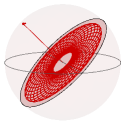
Figure 1: Illustration of the averaging process leading to the VRR equations of motion. For the star S2 around SgrA*, we typically have (Kocsis and Tremaine, 2011) (from left to right): orbital motion $\sim$10 years, pericenter precession $\sim$30,000 years, orbital plane reorientation $\sim$1,000,000 years.

The initial average over the Keplerian motion implies the conservation of the semimajor axis $a$, while the second average results in the conservation of the eccentricity $e$. The shape of each annulus is then described by the conserved quantities ${\mathbf{K}\!=\!(m,a,e)}$, with $m$ the stellar mass. As a result, the norm of each star’s angular momentum, ${L(\mathbf{K})\!=\!m\sqrt{GM_{\bullet}a(1\!-\!e^{2})}}$, is also conserved.

In VRR, the only dynamical quantity is the orbital orientation, which we track via the unit vector, $\widehat{\mathbf{L}}$, with ${\mathbf{L}(\mathbf{K},t)\!=\!L(\mathbf{K})\widehat{\mathbf{L}}(t)}$. The study of VRR reduces then to examining the long-term evolution of each star’s vector $\widehat{\mathbf{L}}$. The dynamics of the system is therefore simplified to the dynamics of $N$ particles on the unit sphere, where each particle represents the instantaneous orientation of an orbital plane associated with a star, see Fig. 2. In this set-up, phase space is the unit sphere (see Appendix A.2).

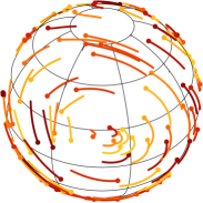
Figure 2: Illustration of VRR, namely $N$ particles evolving on the unit sphere, where each particle represents the orientation of a star’s orbital plane.

As derived in (Kocsis and Tremaine, 2015), after a Legendre expansion of the Newtonian interaction and the use of the addition theorem for spherical harmonics, the VRR total Hamiltonian reads

$$H_{\mathrm{tot}}=-\sum_{i<j}^{N}\sum_{\ell=0}^{+\infty}\sum_{m=-\ell}^{\ell}\mathcal{H}_{\ell}[\mathbf{K}_{i},\mathbf{K}_{j}]\,Y_{\ell m}(\widehat{\mathbf{L}}_{i})\,Y_{\ell m}(\widehat{\mathbf{L}}_{j}).$$ (1)

In that expression, the real spherical harmonics ${Y_{\ell m}(\widehat{\mathbf{L}})}$ are normalized so that ${\!\int\!\mathrm{d}\widehat{\mathbf{L}}Y_{\ell m}Y_{\ell^{\prime}m^{\prime}}\!=\!\delta^{\ell^{\prime}}_{\ell}\delta^{m^{\prime}}_{m}}$, with ${\delta^{\ell^{\prime}}_{\ell}}$ the usual Kronecker symbol. The isotropic coupling coefficients ${\mathcal{H}_{\ell}[\mathbf{K},\mathbf{K}^{\prime}]}$ are spelled out in Appendix A.1. The equations of motion generated by Eq. (1) are also detailed in Appendix A.2.

Following Fouvry et al. (2019), for a given realization, we introduce the empirical distribution function (DF) at time $t$ via

$$\varphi_{\mathrm{d}}(\widehat{\mathbf{L}},\mathbf{K},t)=\sum_{i=1}^{N}\delta_{\mathrm{D}}\big{[}\widehat{\mathbf{L}}\!-\!\widehat{\mathbf{L}}_{i}(t)\big{]}\,\delta_{\mathrm{D}}\big{[}\mathbf{K}\!-\!\mathbf{K}_{i}\big{]},$$ (2)

with $\delta_{\mathrm{D}}$ the usual Dirac delta. The empirical DF satisfies the normalization convention ${\!\int\!\mathrm{d}\widehat{\mathbf{L}}\mathrm{d}\mathbf{K}\,\varphi_{\mathrm{d}}\!=\!N}$. Here, $\varphi_{\mathrm{d}}$ satisfies the continuity equation

$$\partial_{t}\varphi_{\mathrm{d}}(\widehat{\mathbf{L}},\mathbf{K},t)=-\partial_{\widehat{\mathbf{L}}}\!\cdot\!\big{[}\varphi_{\mathrm{d}}(\widehat{\mathbf{L}},\mathbf{K},t)\,\mathrm{d}\widehat{\mathbf{L}}/\mathrm{d}t\big{]},$$ (3)

with ${\mathrm{d}\widehat{\mathbf{L}}/\mathrm{d}t}$ given by Eq. (35). To capture the system’s rotational invariance, we expand the empirical DF in spherical harmonics as follows

$$\varphi_{\mathrm{d}}(\widehat{\mathbf{L}},\mathbf{K},t)=\sum_{a}\varphi_{a}(\mathbf{K},t)\,Y_{a}(\widehat{\mathbf{L}}),$$ (4)

with ${a\!=\!(\ell,m)}$, not to be confused with the mass and semi-major axis previously introduced. The harmonic components ${\varphi_{a}(\mathbf{K},t)}$ are used as tracers of the correlated dynamics occurring in the system. In the context of VRR, the number $\ell$ is formally analogous to the wave vector $|{\textbf{k}}|$ in plasma turbulence (see, e.g., Krommes, 2002), i.e. it describes the typical (inverse) scale of the considered fluctuations.

By expanding in spherical harmonics, Eq. (3) ultimately becomes (see eq. 9 in Fouvry et al. (2019))

$$\partial_{t}\varphi_{a}(\mathbf{K},t){} =\tfrac{1}{2}\sum_{b,c}\!\!\int\!\!\mathrm{d}\mathbf{K}_{b}\mathrm{d}\mathbf{K}_{c}\,\gamma_{abc}[\mathbf{K},\mathbf{K}_{b},\mathbf{K}_{c}]\,$$

$$\times\varphi_{b}(\mathbf{K}_{b},t)\,\varphi_{c}(\mathbf{K}_{c},t),$$ (5)

where we introduced the time-independent non-random bare interaction coefficient, $\gamma_{abc}$, explicitly given in Appendix A.4. This coefficient captures the coupling between different populations and scales, as well as the system’s spherical symmetry. Equation (5) is the master equation on which all the upcoming calculations will be focused.

We now introduce a generalized coordinate that includes time, ${1\!=\!(a,\mathbf{K},t)}$. Equation (5) becomes

$$\partial_{t}\varphi_{1}=\tfrac{1}{2}\,\gamma_{123}\,\varphi_{2}\,\varphi_{3},$$ (6)

where ${\varphi_{a}(\mathbf{K},t)\!=\!\varphi_{1}}$, and integration/summation over repeated variables is assumed. Here, the generalized bare interaction coefficient is symmetric in its last two arguments, i.e. ${\gamma_{123}\!=\!\gamma_{132}}$, and its time dependence is a product of Dirac delta functions (see Appendix A.4).

Equation (6), the evolution equation for $\varphi_{1}$, is deterministic: stochasticity only enters through the initial conditions. In addition, Eq. (6) is local in time, and purely quadratic (it contains no constant or linear terms). The structure of Eq. (6) is very general and can be applied to other systems, such as turbulence in plasmas (see, e.g., Kadomtsev, 1965) or fluids (see, e.g., Frisch and Kolmogorov, 1995), as well as the growth of large scale cosmological structures (see, e.g., Bernardeau et al., 2002).

To characterize the correlated stochastic dynamics of the system, our goal is to investigate the statistical properties of the density fluctuations, $\varphi_{1}$, generated by the $N$ particles, recalling that ${N\!\gg\!1}$. More precisely, we focus on studying the correlation functions of these density fluctuations. In that view, we define the two-point correlation function

$$C_{12}=\langle\varphi_{1}\,\varphi_{2}\rangle-\langle\varphi_{1}\rangle\langle\varphi_{2}\rangle,$$ (7)

where the ensemble average, ${\langle\cdot\rangle}$, is taken over the set of initial conditions. For a (statistically) isotropic system, the mean field is ${\langle\varphi_{1}\rangle\!=\!0}$, as long as ${(\ell_{1},m_{1})\!\neq\!(0,0)}$. Hence, focusing our interest on isotropic VRR, we simply have ${C_{12}\!=\!\langle\varphi_{1}\,\varphi_{2}\rangle}$. Let us note that $C$ is an Eulerian correlation, since its space and time coordinates are specified independently. This differs from its Lagrangian definition, for which the spatial coordinate would be evaluated along the time-dependent trajectory. The goal of this work is to predict $C$.

From Eq. (6), we can derive an evolution equation for $C_{12}$. It reads

$$\partial_{t}C_{12}=\tfrac{1}{2}\,\gamma_{134}\,\langle\varphi_{2}\,\varphi_{3}\,\varphi_{4}\rangle.$$ (8)

The structure of Eq. (8) manifestly raises the question of Gaussianity. For isotropic VRR, fluctuations start mainly Gaussian as a result of the particles’ initial statistical independence. Yet, because one wants ${\partial_{t}C}$ to be non-zero, one must unavoidably take into account the non-Gaussianities arising from the evolution of higher-order cumulants. From Eq. (8), it stems that the evolution equations for the correlations follow a hierarchy that is not self-contained. This issue is famously known as the closure problem (see, e.g., Krommes, 2002). To address this problem, we employ a statistical closure scheme leading to a self-consistent equation for $C$.

III Martin–Siggia–Rose closure

To obtain a time-evolution equation for the two-point correlation function, we follow the MSR formalism Martin et al. (1973). Using techniques from Quantum Field Theory (see, e.g. Lancaster and Blundell, 2014; Peskin and Schroeder, 2018), this approach aims at obtaining a renormalized statistical theory for a classical field satisfying a non-linear dynamical equation, such as Eq. (6). We refer to Krommes (2002) for a particularly extensive and thorough review of the topic of statistical closure theory. Specifically, the present section closely follows section 6.2 of Krommes (2002), whose main details are reproduced below for completeness.

III.1 Field equations of motion

To build a statistical description of the system, it is intuitive to consider both the system’s correlations and its response to infinitesimal fluctuations. This will take the form of self-consistent equations involving the two-point correlation and response.

We introduce the mean response function $R_{12}$, describing the mean response of the system $\varphi$ at point $1$ to a perturbation $\eta$ at point $2$. As a result of causality, it reads

$$R_{12}=\langle\delta\varphi_{1}/\delta\eta_{2}\rangle\big{|}_{\eta=0}\,,\quad\forall\,t_{1}>t_{2}.$$ (9)

Here, $\eta$ is as a non-random external source added to the equation of motion (6). Although explicit, the previous definition does not allow for the derivation of the desired evolution equations, as we want to combine the dynamics of $C$ and $R$ into a single equation. Therefore, an alternative representation of the response is required, i.e. one that gives $R$ the same structure as $C$. This is what the MSR formalism provides. To do so, MSR proceeds by introducing a new operator, $\widehat{\varphi}$, that does not commute with the original field, $\varphi$. A heuristic definition would be ${\widehat{\varphi}\!=\!-\delta/\delta\varphi}$. Importantly, as detailed in Appendix B.2, with the appropriate choice of $\widehat{\varphi}$, Eq. (9) is equivalent to

$$R_{12}=\langle\varphi_{1}\,\widehat{\varphi}_{2}\rangle-\langle\varphi_{1}\rangle\langle\widehat{\varphi}_{2}\rangle,\quad\forall\,t_{1}>t_{2},$$ (10)

to compare with Eq. (7).

From Eq. (6), one can then show that $\widehat{\varphi}$ evolves through ${\partial_{t_{1}}\widehat{\varphi}_{1}\!=\!-\gamma_{231}\,\widehat{\varphi}_{2}\,\varphi_{3}}$. To combine the evolution equations for $\varphi$ and $\widehat{\varphi}$, MSR introduces the spinor indices ${\epsilon\!=\!\pm}$, such that ${\mathbf{1}\!=\!(\epsilon,1)}$. From it, one then defines the two-component field, ${\Phi(+,1)\!=\!\Phi^{\scalebox{0.6}{$+$}}_{1}\!=\!\varphi_{1}}$ and ${\Phi^{\scalebox{0.6}{$-$}}_{1}\!=\!\widehat{\varphi}_{1}}$. The equation of motion for $\Phi$ ultimately takes the compact form (see eq. 3.8 in Martin et al. (1973) and eq. 275 in Krommes (2002))

$$\partial_{t_{1}}\Phi_{\mathbf{1}}=\tfrac{1}{2}\,\varsigma_{\mathbf{1}\mathbf{2}}\,\gamma_{\mathbf{2}\mathbf{3}\mathbf{4}}\,\Phi_{\mathbf{3}}\,\Phi_{\mathbf{4}}.$$ (11)

In that expression, we introduced ${\varsigma_{\mathbf{1}\mathbf{2}}\!=\!\varsigma_{\epsilon_{1}\epsilon_{2}}\delta_{12}}$, with $\varsigma$ a Pauli-like tensor defined in Eq. (54), and ${\delta_{12}\!=\!\delta^{a_{2}}_{a_{1}}\delta_{\mathrm{D}}(\mathbf{K}_{1}\!\!-\!\mathbf{K}_{2})\delta_{\mathrm{D}}(t_{1}\!\!-\!t_{2})}$. Equation (11) involves the generalized non-random bare interaction vertex $\gamma_{\mathbf{1}\mathbf{2}\mathbf{3}}$, defined in Appendix B.1. This vertex is fully symmetric, making Eq. (11) also fully symmetric.

III.2 Generating cumulants

To obtain the correlation and response functions from the field $\Phi$, MSR uses moment and cumulant generating functionals. Importantly, this derivation requires Gaussian initial conditions and non-random coupling coefficients $\gamma$. Such conditions are verified in isotropic VRR, although a generalization is possible (see, e.g., Rose, 1985). In this section, we employ the same notations as in Krommes (2002).

The time-ordered cumulant generating functional is

$$W[\eta]=\ln\,\langle\exp{(\Phi_{\mathbf{1}}\eta_{\mathbf{1}})}\rangle,$$ (12)

where ${\eta\!=\!(\eta^{\scalebox{0.6}{$+$}},\eta^{\scalebox{0.6}{$-$}})}$ is a two-component non-random field. In this context, it is $\varsigma_{\mathbf{1}\mathbf{2}}\eta_{\mathbf{2}}$ that perturbs the evolution equation of $\Phi$, Eq. (11) . From Eq. (12), we define the mean field, ${\langle\varphi\rangle}$, the two-point correlation, $C$, and the mean response function, $R$, as

$$\langle\varphi_{1}\rangle\!=\!\frac{\delta W}{\delta\eta^{\scalebox{0.6}{$+$}}_{1}}\!\bigg{|}_{\eta=0}\!\!\!,\,C_{12}\!=\!\frac{\delta^{2}W}{\delta\eta^{\scalebox{0.6}{$+$}}_{1}\delta\eta^{\scalebox{0.6}{$+$}}_{2}}\!\bigg{|}_{\eta=0}\!\!\!,\,R_{12}\!=\!\frac{\delta^{2}W}{\delta\eta^{\scalebox{0.6}{$+$}}_{1}\delta\eta^{\scalebox{0.6}{$-$}}_{2}}\!\bigg{|}_{\eta=0}\!\!\!.$$ (13)

As detailed in Appendix B.2, starting from this expression for $R$, the time-ordering in Eq. (12) gives Eq. (10).

It is further convenient to reason in terms of cumulants, and compute their equations of motion. For a given $\eta$, cumulants are defined through

$$G_{\mathbf{1}...{\textbf{n}}}=\frac{\delta^{n}W[\eta]}{\delta\eta_{\mathbf{1}}...\delta\eta_{\textbf{n}}}.$$ (14)

When taking ${\eta\!=\!0}$ in Eq. (14), $G_{\mathbf{1}}$ reduces to the mean field, and $G_{\mathbf{1}\mathbf{2}}$ to the desired two-point correlation and response functions. More precisely, we have

$$G^{\scalebox{0.6}{$+$}\scalebox{0.6}{$+$}}_{12}|_{\eta=0}=C_{12};\quad G^{\scalebox{0.6}{$+$}\scalebox{0.6}{$-$}}_{12}|_{\eta=0}=R_{12};$$

$$G^{\scalebox{0.6}{$-$}\scalebox{0.6}{$+$}}_{12}|_{\eta=0}=R_{21};\quad G^{\scalebox{0.6}{$-$}\scalebox{0.6}{$-$}}_{12}|_{\eta=0}=0,$$ (15)

with the notation ${G_{\mathbf{1}\mathbf{2}}\!=\!G^{\scalebox{0.55}{$\epsilon_{1}\epsilon_{2}$}}_{12}}$. Importantly, $G$ is fully symmetric, specifically ${G_{\mathbf{1}\mathbf{2}}\!=\!G_{\mathbf{2}\mathbf{1}}}$. Our goal is now to obtain an evolution equation for $G_{\mathbf{1}\mathbf{2}}$, thus for $C$ and $R$.

III.3 Cumulant evolution equations

Appendix B.4 provides the detailed derivation of the evolution equations for the one-point and two-point cumulants. We first obtain the equation for $G_{\mathbf{1}}$ by differentiating Eq. (14) wrt the time $t_{1}$. Then, from ${G_{\mathbf{1}\mathbf{1}^{\prime}}\!=\!\delta G_{\mathbf{1}}/\delta\eta_{\mathbf{1}^{\prime}}}$ (see Eq. 14), we derive the equation for $G_{\mathbf{1}\mathbf{1}^{\prime}}$ by differentiating ${\partial_{t_{1}}\!G_{\mathbf{1}}}$ wrt $\eta_{\mathbf{1}^{\prime}}$. It reads

$$G_{\mathbf{1}\mathbf{1}^{\prime}}=g_{\mathbf{1}\mathbf{1}^{\prime}}+\tfrac{1}{2}g_{\mathbf{1}\mathbf{2}}\gamma_{\mathbf{2}\mathbf{3}\mathbf{4}}G_{\mathbf{3}\mathbf{4}\mathbf{1}^{\prime}},$$ (16)

with

$$g^{-1}_{\mathbf{1}\mathbf{1}^{\prime}}=-\varsigma_{\mathbf{1}\mathbf{1}^{\prime}}\partial_{t_{1}}-\gamma_{\mathbf{1}\mathbf{1}^{\prime}\mathbf{2}}G_{\mathbf{2}}.$$ (17)

Here, $g$ is to be interpreted as the bare propagator. In the particular case of isotropic VRR, since ${G_{\mathbf{1}}|_{\eta=0}\!=\!0}$, we simply have ${{g^{-1}_{\mathbf{1}\mathbf{1}^{\prime}}}|_{\eta=0}\!=\!-\varsigma_{\mathbf{1}\mathbf{1}^{\prime}}\partial_{t_{1}}}$. Of course, premature setting of ${\eta\!=\!0}$ should be avoided, as it would result in overlooking terms coming from functional derivatives wrt $\eta$. At this stage, it is evident that Eq. (16) is not closed, since $G_{\mathbf{1}\mathbf{2}}$ is sourced by $G_{\mathbf{1}\mathbf{2}\mathbf{3}}$.

III.4 Vertex renormalization

Taking further functional derivatives of Eq. (16) wrt $\eta$ leads to an unclosed statistical hierarchy, in just the same way as in Eq. (8). As stated in Martin et al. (1973), the key step to achieve statistical closure is to perform a Legendre transform from $\eta_{\mathbf{1}}$ to $G_{\mathbf{1}}$ via

$$L[G]=W[\eta]-\eta_{\mathbf{1}}G_{\mathbf{1}}.$$ (18)

From it, we introduce the renormalized vertices as

$$\Gamma_{\mathbf{1}...\mathbf{n}}=\frac{\delta^{n}L[G]}{\delta G_{\mathbf{1}}...\delta G_{\mathbf{n}}},$$ (19)

which are fully symmetric in their coordinates. By taking subsequent functional derivatives of Eq. (18) wrt $G_{\mathbf{1}}$, and knowing that ${G_{\mathbf{1}\mathbf{2}}G_{\mathbf{2}\mathbf{1}^{\prime}}^{-1}\!=\!\delta_{\mathbf{1}\mathbf{1}^{\prime}}}$, we obtain an expression of the three-point vertex as a function of the two-point and three-point cumulants

$$\Gamma_{\mathbf{1}\mathbf{2}\mathbf{3}}=G^{-1}_{\mathbf{1}\mathbf{1}^{\prime}}\,G^{-1}_{\mathbf{2}\mathbf{2}^{\prime}}\,G^{-1}_{\mathbf{3}\mathbf{3}^{\prime}}\,G_{\mathbf{1}^{\prime}\mathbf{2}^{\prime}\mathbf{3}^{\prime}}.$$ (20)

This is detailed in Appendix B.5. Equation (20) involves the three-point cumulant, which sources the dynamics of the two-point cumulant in Eq. (16). Starting from Eq. (16) and using Eq. (20), the MSR closure formula finally takes the form of the Dyson equation

$$G_{\mathbf{1}\mathbf{1}^{\prime}}=g_{\mathbf{1}\mathbf{1}^{\prime}}+g_{\mathbf{1}\mathbf{2}}\Sigma_{\mathbf{2}\mathbf{3}}\,G_{\mathbf{3}\mathbf{1}^{\prime}}.$$ (21)

In Eq. (21), we introduced the self-energy

$$\Sigma_{\mathbf{1}\mathbf{1}^{\prime}}=\tfrac{1}{2}\,\gamma_{\mathbf{1}\mathbf{2}\mathbf{3}}\,G_{\mathbf{2}\mathbf{2}^{\prime}}\,G_{\mathbf{3}\mathbf{3}^{\prime}}\,\Gamma_{\mathbf{1}^{\prime}\mathbf{2}^{\prime}\mathbf{3}^{\prime}},$$ (22)

and the renormalized interaction vertex

$$\Gamma_{\mathbf{1}\mathbf{2}\mathbf{3}}=\gamma_{\mathbf{1}\mathbf{2}\mathbf{3}}+\frac{\delta\Sigma_{\mathbf{1}\mathbf{2}}}{\delta G_{\mathbf{4}\mathbf{5}}}\,G_{\mathbf{4}\mathbf{4}^{\prime}}\,G_{\mathbf{5}\mathbf{5}^{\prime}}\,\Gamma_{\mathbf{3}\mathbf{4}^{\prime}\mathbf{5}^{\prime}},$$ (23)

as outlined in Appendix B.5. Equation (21) is formally exact, since it is a sophisticated rewriting of Eq. (16). Moreover, from Eqs. (21) and (22), we deduce that the target for statistical closure is the determination of the three-point renormalized vertex, $\Gamma_{\mathbf{1}\mathbf{2}\mathbf{3}}$. Indeed, it explicitly depends on the three-point cumulant, $G_{\mathbf{1}\mathbf{2}\mathbf{3}}$ (Eq. 20), which in turn relies on the three-point correlation appearing in Eq. (8). In the present case, the replacement ${g\!\to\!G}$ (resp. ${\gamma\!\to\!\Gamma}$) is analogous to mass (resp. charge) renormalization in Quantum Field Theory (Peskin and Schroeder, 2018).

Imposing ${\eta\!=\!0}$ in Eq. (21), and looking at the ${++}$ and ${+-}$ components of that equation, we obtain

$$\partial_{t_{1}}C_{12}={} \Sigma^{\scalebox{0.6}{$-$}\scalebox{0.6}{$-$}}_{1\,3}R_{23}+\Sigma^{\scalebox{0.6}{$-$}\scalebox{0.6}{$+$}}_{1\,3}C_{32},$$ (24a)

$$\partial_{t_{1}}R_{12}={} \delta_{12}+\Sigma^{\scalebox{0.6}{$-$}\scalebox{0.6}{$+$}}_{1\,3}R_{32}.$$ (24b)

This forms a set of coupled equations for the quantities of interest, that is the two-point correlation, $C$, and the mean response function, $R$. Here, the first term in Eq. (24a) is a “source” term, and depends non-linearly on $C$ and $R$ via Eq. (22). In Eq. (24b), this source term becomes a Dirac delta function to comply with causality. When solving Eqs. (24), an approximation of $\Gamma$ is required, which subsequently determines $\Sigma$ according to Eq. (22).

III.5 Direct Interaction Approximation (DIA)

The DIA was first introduced by Kraichnan (1958), specifically in the context of fluid turbulence. This approach has been extended to other systems Ottaviani (1990); Krommes (2002); Zhou (2021), and it is recovered by the MSR formalism Martin et al. (1973). We refer to Krommes (2002) for a careful historical account of the DIA.

As previously mentioned, one must determine the three-point vertex, $\Gamma_{\mathbf{1}\mathbf{2}\mathbf{3}}$, in order to close Eqs. (21)-(23). In the case of isotropic VRR, we can consider that the characteristic charge of our system is the bare coupling, $\gamma_{\mathbf{1}\mathbf{2}\mathbf{3}}$. It describes how the different populations and different scales couple. From Eqs. (22) and (23), the simplest approximation in that parameter is

$$\Gamma_{\mathbf{1}\mathbf{2}\mathbf{3}}{} =\gamma_{\mathbf{1}\mathbf{2}\mathbf{3}},$$ (25a)

$$\Sigma_{\mathbf{1}\mathbf{1}^{\prime}}{} =\tfrac{1}{2}\,\gamma_{\mathbf{1}\mathbf{2}\mathbf{3}}\,G_{\mathbf{2}\mathbf{2}^{\prime}}\,G_{\mathbf{3}\mathbf{3}^{\prime}}\,\gamma_{\mathbf{1}^{\prime}\mathbf{2}^{\prime}\mathbf{3}^{\prime}}.$$ (25b)

The general (Eulerian) DIA equations are then given by the conjunction of the system of partial differential equations (24) with the approximations from Eqs. (25), complemented with initial conditions for the functions $C$ and $R$.

The DIA is the lowest-order closure scheme in the MSR formalism. In the DIA, the typical amplitude of $\Sigma$ is determined by $\gamma^{2}$. A (naive) higher-order expansion of $\Gamma$ would be to account for the next-order terms in powers of the bare vertex, $\gamma$, by expanding Eq. (23) wrt $\gamma$. In Section IV.4, we explore this simple approach, and show that it produces diverging predictions. This is no surprise since VRR is, in a sense, in the regime of “strong turbulence” (see, e.g. Krommes, 2002), for which renormalizations ought to be more careful. Self-consistent and systematic higher-order approximations (see, e.g. Martin et al., 1973) will be the subject of future research.

IV Application: DIA for VRR

In this section, we tailor the DIA to the case of VRR, and leverage some of the specific properties of this problem. In particular, we rely on time-stationarity and isotropy, to considerably simplify the structure of the equations. In addition, the strictly conservative nature of the system also plays a key role. Finally, we compare the DIA predictions with $N$-body simulations.

IV.1 Stationarity and isotropy

Let us consider an initial distribution of orientations that is statistically isotropic on the unit sphere, and consists of statistically independent stellar populations. In that case, we expect the correlation function to be stationary in time, with an initial value set to ${C_{{12\,|{t_{1}\!=t_{2}}}}\!\!=\!\delta_{a_{1}}^{a_{2}}\delta_{\mathrm{D}}(\mathbf{K}_{1}\!-\!\mathbf{K}_{2})n(\mathbf{K}_{1})}$. Here, ${n(\mathbf{K})}$ is the distribution function of the stars’ parameters $\mathbf{K}$ satisfying ${\int\mathrm{d}\hat{{\textbf{L}}}\mathrm{d}\mathbf{K}n(\mathbf{K})\!=\!N}$ (see Appendix D in Fouvry et al., 2019). Assuming that isotropy is conserved, the correlation can be expanded as

$$C_{12}{} =\delta_{a_{1}}^{a_{2}}\,\delta_{\mathrm{D}}(\mathbf{K}_{1}\!\!-\!\!\mathbf{K}_{2})\,C_{\ell_{1}}(\mathbf{K}_{1},t_{1}\!-\!t_{2}),$$ (26)

and a similar writing holds for ${R_{12}\!\propto\!R_{\ell_{1}}}$, with the initial conditions ${C_{\ell}(\mathbf{K},t\!=\!0)\!=\!n(\mathbf{K})}$ and ${R_{\ell}(\mathbf{K},t\!=\!0)\!=\!1}$. To further limit the complexity hidden in the coupling $\gamma_{\mathbf{1}\mathbf{2}\mathbf{3}}$, we consider from now on the case of a single population system, i.e. a single value of $\mathbf{K}$. In that case, one has ${n(\mathbf{K})\!=\!N/(4\pi)}$, ${R_{\ell}(\mathbf{K},t)\!=\!R_{\ell}(t)}$, ${C_{\ell}(\mathbf{K},t)\!=\!C_{\ell}(t)}$ and ${\mathcal{J}_{\ell}[\mathbf{K},\mathbf{K}^{\prime}]\!=\!\mathcal{J}_{\ell}}$. The multi-population case is briefly explored in Appendix C.

Our goal is now to determine a self-consistent evolution equation for the isotropic correlation function ${t\!\mapsto\!C_{\ell}(t)}$, and compare it with numerical measurements in $N$-body simulations.

IV.2 Fluctuation-Dissipation Theorem

The isotropic VRR is a thermodynamic equilibrium. In addition, the absence of any external forcing or dissipation makes the system strictly conservative. For such a statistical equilibrium, the Fluctuation-Dissipation Theorem (FDT) holds (Kraichnan, 1959b), and ensures that the correlation $C$ is directly proportional to the response function $R$. A detailed discussion of the statistical dynamics of thermal equilibria is provided in section 3.7 of Krommes (2002). The FDT for the stationary problem is also explored in (Ottaviani, 1990).

The FDT in the case of isotropic VRR reads

$$C_{\ell}(t)=C_{0}\,R_{\ell}(|t|),$$ (27)

where ${R_{\ell}(t)\!=\!0}$ for ${t\!<\!0}$ and ${C_{0}\!=\!N/(4\pi)}$. As a reassuring self-consistency check, we explicitly verified that Eq. (27) is an exact solution of the DIA, as governed by Eqs. (24) and (25). In other words, for isotropic VRR, the DIA is fully compatible with the FDT.

As a result of the FDT, Eq. (24b) becomes, ${\forall\ell}$,

$$\partial_{t}R_{\ell}(t){} =-\frac{1}{2\ell\!+\!1}\frac{N}{4\pi}\sum_{\ell_{1},\,\ell_{2}}[\mathcal{J}_{\ell_{1}}\!\!-\!\!\mathcal{J}_{\ell_{2}}][\mathcal{J}_{\ell_{1}}\!\!-\!\!\mathcal{J}_{\ell}](E^{L}_{\ell\,\ell_{1}\ell_{2}})^{2}$$

$$\times\!\!\int^{t}_{0}\!\!\mathrm{d}t^{\prime}R_{\ell_{1}}(t\!-\!t^{\prime})R_{\ell_{2}}(t\!-\!t^{\prime})R_{\ell}(t^{\prime}),$$ (28)

where the ${\mathcal{J}_{\ell}\!=\!\mathcal{H}_{\ell}/L}$ coupling coefficients and the $E^{L}$ Elsasser coefficients are respectively given in Appendix A.1 and A.3. To obtain Eq. (28), we used in particular the contraction rules of the Elsasser coefficients, as detailed in Appendix A.3.2. This offered considerable simplifications. Equation (28) is defined for strictly positive times, ${t\!>\!0}$, with the initial condition ${R_{\ell}(t\!=\!0^{+})\!=\!1}$. Equation (28) is the main result of this paper. Its generalization to a multi-population system is provided in Appendix C.

Let us now comment on the main properties of Eq. (28): (i) it is multi-scale, since different harmonics are coupled to one another; (ii) it is highly non-linear, as the rhs scales like ${(R_{\ell})^{3}}$; (iii) it is stationary in time, as it only involves time differences; (iv) it is non-local in time, since the integrand is evaluated at the delayed time ${t\!-\!t^{\prime}}$; (v) it is isotropic, as all the quantities only depend on the spherical harmonic $\ell$; (vi) because of the exclusion rules of the Elsasser coefficients and the nature of the coupling, $\mathcal{J}_{\ell}$, only a few terms in the double sum over harmonics are non-zero; (vii) the number of stars $N$ can be absorbed in the definition of a new rescaled time, making the equation scale-free in $N$; (viii) for the harmonic ${\ell\!=\!0}$ (resp. ${\ell\!=\!1}$), it yields ${\partial_{t}R_{\ell}\!=\!0}$, ensuring the conservation of the total mass (resp. total angular momentum).

IV.3 Numerical solution and $N$-body simulation

We are now set to compare the DIA predictions with numerical measurements. Since the VRR coupling coefficients typically scale like ${\mathcal{J}_{\ell_{\mathrm{int}}}\!\propto\!1/\ell_{\mathrm{int}}^{2}}$ (see appendix B in Kocsis and Tremaine, 2015), we assume, for simplicity, that only the harmonic ${\ell_{\mathrm{int}}\!=\!2}$ contributes to the pairwise interaction. This quadrupolar model has been shown to encompass most of the physics of VRR (Roupas et al., 2017). In addition, it offers some welcome simplification of the numerics. In Appendix D, we detail our numerical scheme to perform $N$-body simulations of the ${\ell_{\mathrm{int}}\!=\!2}$ model.

In order to numerically solve the integro-differential Eq. (28), we proceed by (i) discretizing time regularly and evaluating the time integral using the trapezoidal rule; (ii) employing a second-order predictor-corrector algorithm to perform the integration per se. Our precise scheme is detailed in Appendix E.

In Fig. 3, we compare the DIA predictions for $R_{\ell}$ (Eq. 28) with $N$-body measurements, for the ${\ell_{\mathrm{int}}\!=\!2}$ interaction model.

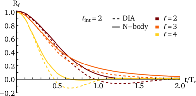
Figure 3: Response function, ${R_{\ell}}$, in the ${\ell_{\mathrm{int}}\!=\!2}$ interaction model, as predicted by the DIA (Eq. 28, dashed lines) and measured in $N$-body simulations (full lines), for the harmonics ${\ell\!=\!2,3,4}$ (different colors). Here, the time has been rescaled by the ballistic time $T_{\mathrm{c}}$, as defined in Eq. (83). On short timescales, the DIA prediction agrees with the measurement, while on longer timescales, it overestimates the decay rate of the fluctuations.

Let us now comment on the main features of this figure.

Here, the harmonics $\ell$ correspond to the angular scales under consideration, with larger $\ell$ corresponding to smaller angular separation between orbits. As could have been expected, in Fig. 3, we find that the smaller the scale, the faster the decorrelation: large scale collective dynamics persist longer than local ones. In that figure, we also find that, for each $\ell$ and for short times, the DIA prediction aligns with the $N$-body measurements, with the initial derivatives matching correctly. However, once decorrelation has started to occur, the DIA prediction seems to underestimate the numerical measurements. In addition, for even harmonics, ${\ell\!=\!2,4}$, the predictions change sign. This is reminiscent of the behavior already observed in fig. 3 of Kraichnan (1961), where the DIA was applied for one of the first times. Yet, given the numerous (and strong) assumptions of the DIA low-order closure scheme, Fig. 3 offers overall a satisfactory result.

In Appendix F, we briefly explore the behavior of the DIA prediction should one account for all the harmonics ${\ell_{\mathrm{int}}\!\geq\!2}$. The associated result is presented in Fig. 6, where we find that a sharper interaction potential leads to faster decorrelations.

IV.4 Higher-order approximation?

In Section III.5, we focused on the DIA, the lowest-order truncation in the MSR formalism. We now briefly discuss the difficulties arising when considering possible higher-order approximations of Eq. (28).

Following Eq. (25), for the DIA, we simply have ${\Gamma\!=\!\gamma}$ and ${\Sigma\!\propto\!\gamma^{2}}$. A naive iteration would be to consider the next-order contribution in $\gamma^{4}$ within the expression of $\Sigma$ from Eq. (22), i.e. to perform an expansion of $\Gamma$ wrt $\gamma$ (Martin et al., 1973; Krommes, 2002; Berera et al., 2013). This approach is particularly simplistic because it assumes that $\gamma$ can be treated as a perturbative parameter and that the expansion actually converges – which can be the case in regimes of “weak turbulence” (see, e.g. Krommes, 2002). Using this approach, the next-order expansion of $\Gamma$ would read

$$\Gamma_{\mathbf{1}\mathbf{2}\mathbf{3}}=\gamma_{\mathbf{1}\mathbf{2}\mathbf{3}}+\gamma_{\mathbf{1}\mathbf{4}\mathbf{5}}G_{\mathbf{4}\mathbf{4}^{\prime}}\gamma_{\mathbf{2}\mathbf{4}^{\prime}\mathbf{6}}G_{\mathbf{5}\mathbf{5}^{\prime}}\,G_{\mathbf{6}\mathbf{6}^{\prime}}\,\gamma_{\mathbf{3}\mathbf{5}^{\prime}\mathbf{6}^{\prime}}.$$ (29)

A diagrammatic representation of Eq. (29) is presented in Fig. 4.

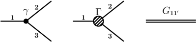
Figure 4: Diagrammatic representation of the MSR formalism. Top: the bare vertex, $\gamma_{\mathbf{1}\mathbf{2}\mathbf{3}}$ (left), the renormalized vertex, $\Gamma_{\mathbf{1}\mathbf{2}\mathbf{3}}$ (middle), and the propagator, $G_{\mathbf{1}\mathbf{1}^{\prime}}$ (right). Bottom: graphical representation of the (naive) next-order expansion from Eq. (29). This expansion is shown to misbehave in Appendix G.

When plugged into Eq. (22), the attempt from Eq. (29) would ultimately lead to an expansion of $\Sigma$ in terms of $\gamma^{2}$ and $\gamma^{4}$, as detailed in Eq. (93). Pushing further the calculation, one can write explicitly the next-order integro-differential equation satisfied by $R_{\ell}$, as given in Eq. (94). When solved numerically, the associated prediction shows signs of strong divergence, as illustrated in Fig. 7. Such a divergence was (somewhat) expected given the inherent naivety of the expansion from Eq. (29). Indeed, it assumes that $\gamma$ can be treated as a meaningful perturbative parameter: this is surely no given in the present regime of isotropic VRR.

As a conclusion, in order to improve upon the DIA prediction from Fig. 3, a more careful and self-consistent next-order renormalization scheme must be implemented to offer a converging prediction. This is discussed in Martin et al. (1973); Krommes (2002), which argue that, in the regime of “strong turbulence”, one should rather expand $\gamma$ in terms of $\Gamma$ (see Fig. 5).

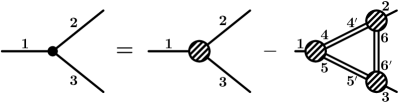
Figure 5: Diagrammatic representation of the improved next-order expansion of the bare vertex, $\gamma_{\mathbf{1}\mathbf{2}\mathbf{3}}$, in powers of the renormalized vertex, $\Gamma_{\mathbf{1}\mathbf{2}\mathbf{3}}$.

Such an improved approach then requires to solve simultaneously joint equations for $\Gamma$ and $G$. This will be the focus of future work.

IV.5 Previous works

It is interesting to compare the present approach to previous methods from the literature on VRR.

A first detailed investigation of the statistics of VRR was made in Kocsis and Tremaine (2015), in particular in section 4 therein. They proceed by introducing two parameters: (i) a ballistic time, $t_{\mathrm{rms}}$, namely the time it would take for the test star to traverse the entire sphere should it feel a constant (and typical) torque (see eq. 71 in Kocsis and Tremaine, 2015); (ii) a decoherence time, $t_{\phi}$, so that on time intervals shorter than $t_{\phi}$, the torque felt by the test star is temporally correlated, while this torque decorrelates on timescales longer than $t_{\phi}$ (see eq. 78 in Kocsis and Tremaine, 2015). Importantly, for isotropic VRR, these two timescales follow the exact same scaling wrt to the total number of particles $N$. VRR is then modeled as a time-correlated random walk on the unit sphere. In particular, Kocsis and Tremaine (2015) recovered both the ballistic and diffusive regimes of diffusion, as illustrated in figs. 10–12 therein. Even if based on motivated heuristics, the approach from Kocsis and Tremaine (2015) recovered all the important qualitative features of the numerical measurements.

The statistics of isotropic VRR was also explored in Fouvry et al. (2019), through the following approximations. First, one computes the initial time-derivative, ${\partial_{t}^{2}C_{\ell}/\partial t^{2}[t\!=\!0]\!\propto\!1/T_{\ell}}$, assuming Gaussian statistics. Second, one approximates the time-dependence of the correlation as a Gaussian, i.e. ${C_{\ell}^{\mathrm{G}}(t)\!\propto\!\mathrm{e}^{-(t/T_{\ell})^{2}/2}}$ (see eq. 23 in Fouvry et al., 2019). Third, one considers the problem of a zero-mass test particle embedded within a Gaussian random noise following the statistics of $C_{\ell}^{\mathrm{G}}$. The correlation of the test particle’s evolution, ${C_{\ell}^{\mathrm{test}}(t)\!\propto\!\langle\varphi_{\ell}^{\mathrm{test}}(0)\varphi^{\mathrm{test}}_{\ell}(t)\rangle}$, is then approximated as ${C_{\ell}^{\mathrm{test}}\!=\!C_{\ell}^{\mathrm{test}}[C_{\ell}^{\mathrm{G}}]}$ (see eq. 33 in Fouvry et al., 2019). Fourth, one introduces back self-consistency, by assuming that the dynamics of each (massive) particle can be approximated by the one of a zero-mass test particle. This leads to a self-consistent relation of the form ${C_{\ell}\!=\!C_{\ell}[C^{\mathrm{test}}]}$ (see eq. 44 in Fouvry et al., 2019). Fouvry et al. (2019) compared their predictions with $N$-body measurements, and could recover the exponential tail of the correlation function, see fig. 3 therein. Unfortunately, it is far from obvious how this approach may be iterated upon to lead ever better approximations. We argue that this is one of the virtues of the present MSR approach, for which systematic higher-order approximations seem within (reasonable) reach.

V Conclusion

In this paper, we investigated the correlated dynamics of VRR, as an archetype of quadratically non-linear stochastic dynamics. In particular, we emphasized how the generic MSR formalism, and its leading order limit, the DIA, can be explicitly implemented to estimate the two-point correlation function of fluctuations. We applied this approach in the isotropic limit of VRR, for which the FDT holds – a welcome simplification. Our main result was obtained in Eq. (28), a fully explicit integro-differential equation for the two-point correlation functions of the fluctuations. This was complemented with Fig. 3, where we compared this prediction with direct measurements in numerical simulations. We found the two approaches to be in satisfactory agreement, though the DIA prediction overestimated the decay rate of the correlation functions.

The present work is only a first step toward a thorough application of statistical closure theory to the problem of VRR. Let us conclude by mentioning a few possible venues for future works.

It surely would be worthwhile to develop the present scheme to the next order. This requires some “vertex renormalization”, i.e. the self-consistent determination of $\Gamma_{\mathbf{1}\mathbf{2}\mathbf{3}}$ (see fig. 3 in Martin et al., 1973), contrary to the DIA which sets it to the bare vertex (see Eq. 25a). While more challenging, we expect for this calculation to remain (reasonably) tractable. For instance, we expect the FDT to hold at any order, as a direct consequence of the thermodynamic equilibrium that is isotropic VRR.

Naturally, a legitimate question is to wonder whether this approach can be further iterated upon, ad libitum. Yet, this is unfortunately not given for the MSR formalism. Indeed, in the absence of any small parameter controlling clearly the order of the expansion, iterations on the MSR scheme may, in a similar fashion to Section IV.4, diverge at higher order (see, e.g., fig. 5 in Kraichnan, 1961). In that context, one could investigate the possibility of more intricate higher-order renormalizations using $n$-body functions and the associated Bethe–Salpeter equations (see, e.g., eq. 234 in (Krommes, 1984) and section 3.1 in (Fukuda et al., 1995)), and $n$-particule irreducible effective actions (see, e.g., Cornwall et al., 1974; Berges, 2004; Carrington and Guo, 2011).

Equation (6), the fundamental evolution equation for VRR, drives some form of cascade between large and small scales, as does Eq. (28). For example, as noted in Fig. 3, large $\ell$, i.e. smaller scales, decorrelate faster. In addition, given that the VRR interaction is dominated by the (large-scale) quadrupolar ${\ell_{\mathrm{int}}\!=\!2}$ interaction, the dynamics of some given harmonics, $\ell$, is dominated by the interaction of the (squeezed) triplets of scales ${\{\ell,\ell_{1},\ell_{2}\}\!\sim\!\{\ell,2,\ell\!\pm\!1\}}$. In that context, it would be interesting to investigate the applicability of “renormalization group” methods (see, e.g., Zhou, 2010, for a review) to VRR.

Similarly, one should also investigate the use of methods stemming from the “non-perturbative functional renormalization group” (see, e.g., Delamotte, 2012; Dupuis et al., 2021, for a review). In this approach, contributions from ever larger scales are progressively accounted for by adding a carefully chosen “regulator” to the system’s action. Interestingly, Tarpin et al. (2019) used such an approach to predict the two-point correlation function in the related context of stationary and isotropic two-dimensional turbulence. On that front, the similarities between eq. (59) of Tarpin et al. (2019) and the VRR result given in eq. (33) of Fouvry et al. (2019) are particularly striking.

Finally, in the astrophysical context, it would be interesting to consider more realistic setups, by alleviating some of our simplifying assumptions. In particular, in no specific order, one should: (i) go beyond the assumption of a statistically isotropic distribution of orientations (see, e.g, Roupas et al., 2017; Touma et al., 2019; Gruzinov et al., 2020); (ii) consider the impact of different stellar populations, e.g., different masses, possibly leading to the spontaneous formation of stellar discs (see, e.g., Szölgyén and Kocsis, 2018; Magnan et al., 2022; Máthé et al., 2023); (iii) investigate the role played by different harmonics contributing to the gravitational coupling (Takács and Kocsis, 2018); (iv) account for the central BH’s relativistic Lense–Thirring precession (see, e.g., Fragione and Loeb, 2022); (v) characterize the impact of a possible intermediate mass BH also orbiting within the system (GRAVITY Collaboration et al., 2023; Will et al., 2023); (vi) investigate the relaxation of a single (zero-mass) test star embedded in this fluctuating system (Kocsis and Tremaine, 2015; Fouvry et al., 2019); (vii) examine the importance of the dynamical friction undergone by a massive test particle in this environment (Ginat et al., 2023); (viii) describe the respective diffusion of two test stars away from one another, i.e. “neighbor separation” (Giral Martínez et al., 2020). Overall, the goal of these various developments would be to use the observation of the (clockwise) stellar disc around SgrA* (see, e.g., Paumard et al., 2006; Bartko et al., 2009; Lu et al., 2009; Yelda et al., 2014; Gillessen et al., 2017; von Fellenberg et al., 2022) along with a precise characterization of VRR to constrain the content of SgrA*’s stellar cluster (see, e.g., Panamarev and Kocsis, 2022; Fouvry et al., 2023).

Appendix A Vector Resonant Relaxation

A.1 Coupling coefficients

Following Magnan et al. (2022) and references therein, the coupling coefficients appearing in Eq. (1) read

$$\mathcal{H}_{\ell}[\mathbf{K},\mathbf{K}^{\prime}]\!=\!\frac{4\pi Gmm^{\prime}}{2\ell\!\!+\!\!1}|P_{\ell}(0)|^{2}\!\!\int_{0}^{\pi}\!\!\frac{\mathrm{d}M}{\pi}\frac{\mathrm{d}M^{\prime}}{\pi}\!\frac{\mathrm{Min}[r,r^{\prime}]^{\ell}}{\mathrm{Max}[r,r^{\prime}]^{\ell+1}},$$ (30)

with $P_{\ell}$ the Legendre polynomial of order $\ell$ and ${(M,M^{\prime})}$ the mean anomalies of the orbits. We note that (i) all odd harmonics $\ell$ are associated with ${\mathcal{H}_{\ell}\!=\!0}$; (ii) the harmonic ${\ell\!=\!0}$ does not drive any dynamics; (iii) the coefficients satisfy the symmetry ${\mathcal{H}_{\ell}[\mathbf{K},\mathbf{K}^{\prime}]\!=\!\mathcal{H}_{\ell}[\mathbf{K}^{\prime},\mathbf{K}]}$.

To simplify the writing, it is convenient to also introduce the rescaled coupling coefficients

$$\mathcal{J}_{\ell}[\mathbf{K},\mathbf{K}^{\prime}]=\mathcal{H}_{\ell}[\mathbf{K},\mathbf{K}^{\prime}]/L(\mathbf{K}),$$ (31)

used later in Eq. (42).

A.2 Equations of motions

Following Kocsis and Tremaine (2015), the dynamics of a given (zero-mass) test particle is given by the effective Hamiltonian

$$H_{\mathrm{test}}=-\sum_{i=1}^{N}\sum_{a}\mathcal{H}_{a}[\mathbf{K},\mathbf{K}_{i}]\,Y_{a}(\widehat{\mathbf{L}})\,Y_{a}(\widehat{\mathbf{L}}_{i}),$$ (32)

with ${a\!=\!(\ell,m)}$.

Let us now introduce the usual ${(\theta,\phi)}$ spherical coordinates. Because of the double orbit-average from Eq. (32), we may track the evolution with the canonical coordinates, ${(\phi,L_{z}\!=\!L\cos\theta)}$. As a result, for VRR, phase space is the unit sphere. The individual equations of motion are given by Hamilton’s equations

$$\frac{\mathrm{d}\phi}{\mathrm{d}t}=\frac{\partial H_{\mathrm{test}}}{\partial L_{z}};\quad\frac{\mathrm{d}L_{z}}{\mathrm{d}t}=-\frac{\partial H_{\mathrm{test}}}{\partial\phi}.$$ (33)

Introducing the operator

$$\widehat{\mathbf{L}}\times\frac{\partial}{\partial\widehat{\mathbf{L}}}={\textbf{e}}_{r}\!\times\!\left\{\frac{\partial}{\partial\theta}{\textbf{e}}_{\theta}+\frac{1}{\sin{\theta}}\frac{\partial}{\partial\phi}{\textbf{e}}_{\phi}\right\},$$ (34)

within the basis ${({\textbf{e}}_{r},{\textbf{e}}_{\theta},{\textbf{e}}_{\phi})}$, we get from Eq. (33)

$$\frac{\mathrm{d}\widehat{\mathbf{L}}}{\mathrm{d}t}=-\frac{1}{L[\mathbf{K}]}\,\widehat{\mathbf{L}}\!\times\!\frac{\partial H_{\mathrm{test}}}{\partial\widehat{\mathbf{L}}}.$$ (35)

This equation of motion is the one appearing in Eq. (3).

A.3 Elsasser coefficients

A.3.1 Definition

Following appendix B in Fouvry et al. (2019), the Elsasser coefficients are defined with the convention

$$E_{abc}=\!\!\int\!\!\mathrm{d}\widehat{\mathbf{L}}\,Y_{a}(\widehat{\mathbf{L}})\,\mathbf{X}_{b}(\widehat{\mathbf{L}})\!\cdot\!\frac{\partial Y_{c}(\widehat{\mathbf{L}})}{\partial\widehat{\mathbf{L}}},$$ (36)

with ${a\!=\!(\ell,m)}$ and the (real) vector spherical harmonics, ${\mathbf{X}_{a}\!=\!\widehat{\mathbf{L}}\!\times\!\partial Y_{a}(\widehat{\mathbf{L}})/\partial\widehat{\mathbf{L}}}$, with ${\partial/\partial\widehat{\mathbf{L}}}$ given in Eq. (34). These coefficients are generically decomposed in (Fouvry et al., 2019)

$$E_{abc}=E^{L}_{\ell_{a}\ell_{b}\ell_{c}}\,E^{M}_{m_{a}m_{b}m_{c}}.$$ (37)

The $E^{M}$ (resp. $E^{L}$) coefficients are antisymmetric (resp. symmetric) when any two indices are transposed. Remarkably, the coefficients $E_{abc}$ are zero unless all pairs ${(\ell,m)}$ are different and

$$|\ell_{a}\!-\!\ell_{b}|<\ell_{c}<\ell_{a}\!+\!\ell_{b}\;\;\text{and}\;\;\ell_{a}\!+\!\ell_{b}\!+\!\ell_{c}\;\text{is odd}.$$ (38)

A.3.2 Contraction rules

We follow Chap. 12 of Varshalovich et al. (1988) to obtain appropriate contraction rules for the anisotropic Elsasser coefficients.

To obtain Eq. (28), we use the identity

$$\sum_{\mathclap{m_{c},m_{d}}}E^{M}_{acd}\,E^{M}_{bcd}=\frac{\delta_{a}^{b}}{2\ell_{a}+1},$$ (39)

where, importantly, it is assumed that all the interaction pairs appearing in Eq. (39), i.e. ${(a,c,d)}$ and ${(b,c,d)}$, satisfy the criteria from Eq. (38).

To derive the (naive) higher-order approximation from Eq. (94), we use the relation

$$\sum_{\mathclap{\begin{subarray}{c}m_{c},m_{d}\\ m_{e},m_{f}\\ m_{g}\end{subarray}}}E^{M}_{acd}\,E^{M}_{bef}\,E^{M}_{gcf}\,E^{M}_{ged}=\frac{\delta_{a}^{b}}{2\ell_{a}\!+\!1}W^{\ell_{a}\,\ell_{c}\,\ell_{d}}_{\ell_{g}\,\ell_{e}\,\ell_{f}},$$ (40)

where we introduced Wigner’s ${6j}$ symbols

$$W^{\ell_{a}\,\ell_{c}\,\ell_{d}}_{\ell_{g}\,\ell_{e}\,\ell_{f}}=(-1)^{\ell_{c}+\ell_{e}}\scalebox{0.9}{$\begin{Bmatrix}\ell_{a}&\ell_{c}&\ell_{d}\\ \ell_{g}&\ell_{e}&\ell_{f}\end{Bmatrix}$}.$$ (41)

Here again, all the triplets of interaction appearing in Eq. (40) must satisfy the conditions from Eq. (38).

A.4 Bare interaction coefficient

The non-random bare interaction coefficient appearing in Eq. (5) is generically given by

$$\gamma_{abc}[\mathbf{K},\mathbf{K}_{b},\mathbf{K}_{c}]=E_{abc}\,\big{\{}{} \mathcal{J}_{\ell_{c}}[\mathbf{K},\mathbf{K}_{c}]\delta_{\mathrm{D}}\big{[}\mathbf{K}\!\!-\!\!\mathbf{K}_{b}\big{]}$$

$$-{} \mathcal{J}_{\ell_{b}}[\mathbf{K},\mathbf{K}_{b}]\delta_{\mathrm{D}}\big{[}\mathbf{K}\!\!-\!\!\mathbf{K}_{c}\big{]}\big{\}},$$ (42)

with $\mathcal{J}_{\ell}$ provided by Eq. (31).

Including the time coordinate as ${1\!=\!(a,\mathbf{K},t)}$, the generalized bare interation coefficient from Eq. (6) is then

$$\gamma_{123}=\gamma_{abc}[\mathbf{K},\mathbf{K}_{b},\mathbf{K}_{c}]\,\delta_{\mathrm{D}}(t\!-\!t_{b})\,\delta_{\mathrm{D}}(t\!-\!t_{c}).$$ (43)

It is symmetric in its last to arguments, i.e. ${\gamma_{123}\!=\!\gamma_{132}}$.

Appendix B Martin-Siggia-Rose Closure

B.1 Bare interaction vertex

In Eq. (11), we introduce the generalized coordinate ${\mathbf{1}\!=\!(\epsilon,1)}$ with ${\epsilon\!=\!\pm}$. The bare interaction vertex reads

$$\gamma_{\mathbf{1}\mathbf{2}\mathbf{3}}={} \tfrac{1}{2}\big{\{}\gamma_{123}\!+\!\gamma_{132}\big{\}}\,\delta_{\epsilon_{1}}^{-}\,\delta_{\epsilon_{2}}^{+}\delta_{\epsilon_{3}}^{+}$$

$$+{} \tfrac{1}{2}\big{\{}\gamma_{213}\!+\!\gamma_{231}\big{\}}\,\delta_{\epsilon_{2}}^{-}\,\delta_{\epsilon_{1}}^{+}\,\delta_{\epsilon_{3}}^{+}$$

$$+{} \tfrac{1}{2}\big{\{}\gamma_{321}\!+\!\gamma_{312}\big{\}}\,\delta_{\epsilon_{3}}^{-}\,\delta_{\epsilon_{2}}^{+}\,\delta_{\epsilon_{1}}^{+}.$$ (44)

Importantly, $\gamma_{\mathbf{1}\mathbf{2}\mathbf{3}}$ is fully symmetric in its arguments, i.e. it is left unchanged by any permutation of two indices.

B.2 Response function

In this appendix, we closely follow section 5.5.6 of Krommes (1984). To precisely define the system’s response to an infinitesimal fluctuation $\eta$, we rewrite the equation of motion Eq. (6) for the distribution function $\varphi$, while adding an external source $\eta$. This reads

$$\partial_{t}\varphi_{1}=\tfrac{1}{2}\,\gamma_{123}\,\varphi_{2}\,\varphi_{3}+\eta_{1},$$ (45)

where $\eta_{1}$ corresponds to $\eta^{\scalebox{0.6}{$-$}}_{1}$ defined in Eq. (12). Let us now define the stochastic response function, describing the response of the system at point $1$ to an infinitesimal fluctuation at point $1^{\prime}$. It reads

$$\widetilde{R}_{11^{\prime}}=\delta\varphi_{1}/\delta\eta_{1^{\prime}}\big{|}_{\eta=0}\quad\forall\,t_{1}>t_{1^{\prime}}.$$ (46)

By differentiating Eq. (45) wrt $\eta_{1^{\prime}}$, we obtain

$$\partial_{t}\widetilde{R}_{11^{\prime}}=\tfrac{1}{2}\,\gamma_{123}\,(\varphi_{2}\widetilde{R}_{31^{\prime}}+\widetilde{R}_{21^{\prime}}\varphi_{3})+\delta_{11^{\prime}}.$$ (47)

Although the definition in Eq. (46) is explicit, it is not practical since the quantity of real interest is the mean response function ${R\!=\!\langle\widetilde{R}\rangle}$. Averaging Eq. (47) would result in intricate terms like ${\langle\varphi\widetilde{R}\rangle}$. Therefore, an alternative representation of the response function is preferred. Specifically, one that gives $R$ the same structure as $C$, for these two quantities to be conjugate.

In the MSR formalism, the key idea is to introduce the operator $\widehat{\varphi}$ through the canonical commutation relation

$$[\varphi({\underline{1}},t);\widehat{\varphi}({\underline{1}}^{\prime},t)]=\delta_{{\underline{1}}\,{\underline{1}}^{\prime}},$$ (48)

where the time coordinate is excluded by defining ${1\!=\!({\underline{1}},t)}$ and ${[A;B]\!=\!AB\!-\!BA}$. This relation is analogous to ${[q;p]\!=\!\mathrm{i}\hbar}$ in Quantum Mechanics, with $q$ the position and ${p\!=\!-\mathrm{i}\hbar\partial_{q}}$ the momentum (see, e.g., Binney and Skinner, 2013). An equivalent path-integral formulation of MSR is reviewed in section 6.4 of Krommes (2002).

We further introduce

$$\widetilde{r}_{11^{\prime}}=\Theta(t-t^{\prime})[\varphi_{1};\widehat{\varphi}_{1^{\prime}}],$$ (49)

with $\Theta$ the usual Heaviside function. Using Eqs. (6) and (48) along with the identity ${[AB;C]\!=\!A[B;C]\!+\![A;C]B}$, we get

$$\partial_{t}\widetilde{r}_{11^{\prime}}=\tfrac{1}{2}\,\gamma_{123}\,(\varphi_{2}\widetilde{r}_{31^{\prime}}+\widetilde{r}_{21^{\prime}}\varphi_{3})+\delta_{11^{\prime}}.$$ (50)

Even though $\widetilde{R}$ and $\widetilde{r}$ satisfy the same evolution equation, we cannot simply state that ${\widetilde{R}\!=\!\widetilde{r}}$. Indeed, the operator $\widetilde{r}$ does not commute with $\varphi$, whereas $\widetilde{R}$ does. However, as argued in Krommes (1984), these two quantities are equal when ensemble-averaged, i.e. ${r\!=\!\langle\widetilde{r}\rangle\!=\!R}$, provided (i) an appropriate definition of the operator $\widehat{\varphi}$ and (ii) the condition ${\langle\widehat{\varphi}\,...\rangle\!=\!0}$ is satisfied, where “${...}$” is any combination of $\varphi$ and $\widehat{\varphi}$ . The mean response function is then given by

$$R_{11^{\prime}}=\Theta(t-t^{\prime})\langle[\varphi_{1};\widehat{\varphi}_{1^{\prime}}]\rangle=\Theta(t-t^{\prime})\langle\varphi_{1}\,\widehat{\varphi}_{1^{\prime}}\rangle.$$ (51)

From ${\langle\widehat{\varphi}\rangle\!=\!0}$, we can write

$$R_{11^{\prime}}{} =\langle\varphi_{1}\,\widehat{\varphi}_{1^{\prime}}\rangle-\langle\varphi_{1}\rangle\langle\widehat{\varphi}_{1^{\prime}}\rangle,\quad\forall\;t>t^{\prime},$$ (52a)

$$C_{11^{\prime}}{} =\langle\varphi_{1}\,\varphi_{1^{\prime}}\rangle-\langle\varphi_{1}\rangle\langle\varphi_{1^{\prime}}\rangle,\quad\forall\;t\,,t^{\prime}.$$ (52b)

We thus have a clear symmetric writing between the two-point correlation, $C$, and the mean response function, $R$. Equations (52a) and (52b) are completely equivalent to the expressions given in Eq. (13).

B.3 Field equations

The commutation relation for the generalized two-component field $\Phi$ follows from Eq. (48). It reads

$$[\Phi(\epsilon_{1},{\underline{1}},t);\Phi(\epsilon_{2},{\underline{2}},t)]=\varsigma_{\epsilon_{1}\epsilon_{2}}\delta_{{\underline{1}}\,{\underline{2}}},$$ (53)

with the Pauli-like tensor, $\varsigma$, appearing in Eq. (11),

$$\varsigma_{\scalebox{0.6}{$+$}\scalebox{0.6}{$+$}}=0;\quad\quad\varsigma_{\scalebox{0.6}{$+$}\scalebox{0.6}{$-$}}=1;$$

$$\varsigma_{\scalebox{0.6}{$-$}\scalebox{0.6}{$+$}}=-1;\,\quad\varsigma_{\scalebox{0.6}{$-$}\scalebox{0.6}{$-$}}=0.$$ (54)

B.4 Cumulant dynamics

In this appendix, we explicitly derive evolution equations for the one-point and two-point cumulants $G_{\mathbf{1}}$ and $G_{\mathbf{1}\mathbf{2}}$. We follow the approach from Krommes (2002). From Eq. (14), we have

$$G_{\mathbf{1}}=\frac{\delta W[\eta]}{\delta\eta_{\mathbf{1}}}=\frac{\langle\Phi_{\mathbf{1}}\exp{(\Phi_{\mathbf{2}}\eta_{\mathbf{2}})}\rangle}{\langle\exp{(\Phi_{\mathbf{2}}\eta_{\mathbf{2}})}\rangle}.$$ (55)

Separating the time coordinate like ${\mathbf{1}\!=\!({\underline{\mathbf{1}}},t)}$, and dealing carefully with time-ordering (from right to left Martin et al. (1973)), we can write

$$\partial_{t}\langle\Phi({\underline{\mathbf{1}}},t)\exp{(\Phi_{\mathbf{2}}\eta_{\mathbf{2}})}\rangle{} =\partial_{t}\langle\exp{[\scalebox{0.95}{$\int^{\infty}_{t}$}\mathrm{d}t^{\prime}\Phi({\underline{\mathbf{2}}},t^{\prime})\eta({\underline{\mathbf{2}}},t^{\prime})]}$$

$$\!\!\!\!\!\!\!\!\times\Phi({\underline{\mathbf{1}}},t)\exp{[\scalebox{0.95}{$\int^{t}_{-\infty}$}\mathrm{d}t^{\prime}\Phi({\underline{\mathbf{2}}},t^{\prime})\eta({\underline{\mathbf{2}}},t^{\prime})]}\rangle$$

$$=\langle\dot{\Phi}({\underline{\mathbf{1}}},t)\exp{[\Phi_{\mathbf{2}}\,\eta_{\mathbf{2}}]}\rangle$$

$$+\langle[-\Phi({\underline{\mathbf{2}}},t)\eta({\underline{\mathbf{2}}},t)\Phi({\underline{\mathbf{1}}},t)$$ (56)

$$+\Phi({\underline{\mathbf{1}}},t)\Phi({\underline{\mathbf{2}}},t)\eta({\underline{\mathbf{2}}},t)]\exp{[\Phi_{\mathbf{2}}\,\eta_{\mathbf{2}}]}\rangle.$$

Using the commutation relation from Eq. (53), we get

$$\partial_{t}G({\underline{\mathbf{1}}},t){} =\frac{\langle\dot{\Phi}({\underline{\mathbf{1}}},t)\exp(\Phi_{\mathbf{2}}\eta_{\mathbf{2}})\rangle}{\langle\exp{(\Phi_{\mathbf{2}}\eta_{\mathbf{2}})\rangle}}+\varsigma\eta({\underline{\mathbf{1}}},t),$$ (57)

where ${\varsigma\eta({\underline{\mathbf{1}}},t)\!=\!\varsigma_{\epsilon_{1}\epsilon_{2}}\eta(\epsilon_{2},{\underline{1}},t)}$. We now note that

$$G_{\mathbf{3}}G_{\mathbf{4}}+G_{\mathbf{3}\mathbf{4}}=\frac{\langle\Phi_{\mathbf{3}}\Phi_{\mathbf{4}}\exp{(\Phi_{\mathbf{5}}\eta_{\mathbf{5}})}\rangle}{\langle\exp{(\Phi_{\mathbf{5}}\eta_{\mathbf{5}})}\rangle},$$ (58)

and inject Eq. (11) into Eq. (57) to obtain

$$\partial_{t}G_{\mathbf{1}}=\tfrac{1}{2}\varsigma_{\mathbf{1}\mathbf{2}}\gamma_{\mathbf{2}\mathbf{3}\mathbf{4}}\big{(}G_{\mathbf{3}}G_{\mathbf{4}}+G_{\mathbf{3}\mathbf{4}}\big{)}+\varsigma\eta_{\mathbf{1}}.$$ (59)

Here, one should pay attention to the source term ${\varsigma\eta_{\mathbf{1}}}$ stemming from time-ordering. Since ${G_{\mathbf{1}\mathbf{1}^{\prime}}\!=\!\delta G_{\mathbf{1}}/\delta\eta_{\mathbf{1}^{\prime}}}$ (see Eq. 14), differentiating Eq. (59) wrt $\eta_{\mathbf{1}^{\prime}}$ yields

$$\partial_{t_{1}}G_{\mathbf{1}\mathbf{1}^{\prime}}=\varsigma_{\mathbf{1}\mathbf{2}}\gamma_{\mathbf{2}\mathbf{3}\mathbf{4}}G_{\mathbf{3}}G_{\mathbf{4}\mathbf{1}^{\prime}}+\tfrac{1}{2}\varsigma_{\mathbf{1}\mathbf{2}}\gamma_{\mathbf{2}\mathbf{3}\mathbf{4}}G_{\mathbf{3}\mathbf{4}\mathbf{1}^{\prime}}+\varsigma_{\mathbf{1}\mathbf{1}^{\prime}}.$$ (60)

Introducing the identity tensor ${\delta_{\mathbf{1}\mathbf{1}^{\prime}}\!=\!-\varsigma_{\mathbf{1}\mathbf{2}}\varsigma_{\mathbf{2}\mathbf{1}^{\prime}}}$, we can rewrite Eq. (60) as

$$G_{\mathbf{1}\mathbf{1}^{\prime}}=g_{\mathbf{1}\mathbf{1}^{\prime}}+\tfrac{1}{2}g_{\mathbf{1}\mathbf{2}}\gamma_{\mathbf{2}\mathbf{3}\mathbf{4}}G_{\mathbf{3}\mathbf{4}\mathbf{1}^{\prime}},$$ (61)

with

$$g^{-1}_{\mathbf{1}\mathbf{1}^{\prime}}=-\varsigma_{\mathbf{1}\mathbf{1}^{\prime}}\partial_{t_{1}}-\gamma_{\mathbf{1}\mathbf{1}^{\prime}\mathbf{2}}G_{\mathbf{2}}.$$ (62)

B.5 Vertex calculation

We compute in this appendix the first vertices, as introduced in Eq. (19). To do so, we take subsequent functional derivatives wrt $G_{\mathbf{1}}$ of the Legendre transform $L$ defined in Eq. (18). Considering that the quantity ${W[\eta]}$ only depends on $G_{\mathbf{1}}$ through the mapping ${\eta_{\mathbf{1}}\!\rightarrow\!G_{\mathbf{1}}}$, we can write ${\delta/\delta G_{\mathbf{1}}\!=\!\delta/\delta\eta_{\mathbf{2}}\big{|}_{G_{\mathbf{1}}}\!\delta\eta_{\mathbf{2}}/\delta G_{\mathbf{1}}}$. It follows

$$\Gamma_{\mathbf{1}}{} =\frac{\delta W[\eta]}{\delta\eta_{\mathbf{2}}}\frac{\delta\eta_{\mathbf{2}}}{\delta G_{\mathbf{1}}}-\frac{\delta\eta_{\mathbf{2}}}{\delta G_{\mathbf{1}}}G_{\mathbf{2}}-\eta_{\mathbf{1}}=-\eta_{\mathbf{1}},$$ (63a)

$$\Gamma_{\mathbf{1}\mathbf{2}}{} =-\frac{\delta\eta_{\mathbf{2}}}{\delta G_{\mathbf{1}}}=-G^{-1}_{\mathbf{1}\mathbf{2}}.$$ (63b)

Let us now calculate the three-point vertex $\Gamma_{\mathbf{1}\mathbf{2}\mathbf{3}}$, as given by Eq. (20). First, we differentiate Eq. (63b) wrt ${G_{\mathbf{3}}}$ to write

$$\Gamma_{\mathbf{1}\mathbf{2}\mathbf{3}}=-\frac{\delta G^{-1}_{\mathbf{1}\mathbf{2}}}{\delta G_{\mathbf{3}}}.$$ (64)

To make progress, we use the identity operator

$$G_{\mathbf{1}\mathbf{2}}\,G^{-1}_{\mathbf{2}\mathbf{1}^{\prime}}=\delta_{\mathbf{1}\mathbf{1}^{\prime}}.$$ (65)

Multiplying Eq. (65) on the left by $G$ and differentiating it wrt $\eta$ yields

$$G_{\mathbf{1}\mathbf{1}^{\prime}}\,G_{\mathbf{2}\mathbf{2}^{\prime}}\frac{\delta G^{-1}_{\mathbf{1}\mathbf{2}}}{\delta\eta_{\mathbf{3}^{\prime}}}=-G_{\mathbf{1}^{\prime}\mathbf{2}^{\prime}\mathbf{3}^{\prime}}.$$ (66)

Then, noting that

$$\frac{\delta G^{-1}_{\mathbf{1}\mathbf{2}}}{\delta G_{\mathbf{3}}}=\frac{\delta G^{-1}_{\mathbf{1}\mathbf{2}}}{\delta\eta_{\mathbf{3}^{\prime}}}\frac{\delta\eta_{\mathbf{3}^{\prime}}}{\delta G_{\mathbf{3}}},$$ (67)

since $G^{-1}_{\mathbf{1}\mathbf{2}}$ depends on $G_{\mathbf{3}}$ through $\eta$, we ultimately obtain

$$\Gamma_{\mathbf{1}\mathbf{2}\mathbf{3}}=G^{-1}_{\mathbf{1}\mathbf{1}^{\prime}}\,G^{-1}_{\mathbf{2}\mathbf{2}^{\prime}}\,G^{-1}_{\mathbf{3}\mathbf{3}^{\prime}}\,G_{\mathbf{1}^{\prime}\mathbf{2}^{\prime}\mathbf{3}^{\prime}}.$$ (68)

We now want to derive the expression of the three-point vertex given in Eq. (23). To do so, we start from the Dyson equation (21)

$$G^{-1}_{\mathbf{1}\mathbf{2}}=g^{-1}_{\mathbf{1}\mathbf{2}}-\Sigma_{\mathbf{1}\mathbf{2}},$$ (69)

and differentiate it wrt $G_{\mathbf{3}}$, thus giving

$$\Gamma_{\mathbf{1}\mathbf{2}\mathbf{3}}=\gamma_{\mathbf{1}\mathbf{2}\mathbf{3}}+\frac{\delta\Sigma_{\mathbf{1}\mathbf{2}}}{\delta G_{\mathbf{3}}}.$$ (70)

In Eq. (70), we used the definition from Eq. (17). Assuming from Eqs. (70) and (22) that $\Sigma_{\mathbf{1}\mathbf{2}}$ depends on $G_{\mathbf{3}}$ only explicitly through $G_{\mathbf{4}\mathbf{5}}$ (see section 6.2.3 in Krommes, 2002), we may write

$$\frac{\delta\Sigma_{\mathbf{1}\mathbf{2}}}{\delta G_{\mathbf{3}}}\bigg{|}_{\eta}\!\!=\!\frac{\delta\Sigma_{\mathbf{1}\mathbf{2}}}{\delta G_{\mathbf{4}\mathbf{5}}}\bigg{|}_{G_{\mathbf{3}}}\!\!\frac{\delta G_{\mathbf{4}\mathbf{5}}}{\delta G_{\mathbf{3}}}\bigg{|}_{\eta}\!\!=\!\frac{\delta\Sigma_{\mathbf{1}\mathbf{2}}}{\delta G_{\mathbf{4}\mathbf{5}}}G_{\mathbf{4}\mathbf{4}^{\prime}}G_{\mathbf{5}\mathbf{5}^{\prime}}\Gamma_{\mathbf{3}\mathbf{4}^{\prime}\mathbf{5}^{\prime}},$$ (71)

where we used the identity from Eq. (65). Plugging Eq. (71) into Eq. (70) yields Eq. (23).

Appendix C Multi-population and DIA

In the case of a multi-population system, the FDT from Eq. (27) becomes

$$C_{\ell}({\textbf{K}},t)=n(\mathbf{K})R_{\ell}(\mathbf{K},|t|),$$ (72)

with ${n(\mathbf{K})}$ the distribution function of the stars’ parameters, ${\mathbf{K}\!=\!(m,a,e)}$.

After some manipulations, the equivalent of Eq. (28) for a multi-population system is

$$\partial_{t}R_{\ell}({\textbf{K}},t)$$

$$=\!-\frac{1}{2\ell+1}\!\!\sum_{\ell_{1},\ell_{2}}\!\!\int_{0}^{t}\!\!\mathrm{d}t^{\prime}\!\!\int\!\!\mathrm{d}{\textbf{K}}^{\prime}\!\bigg{[}n({\textbf{K}}^{\prime})\mathcal{J}_{\ell_{1}}[{\textbf{K}},{\textbf{K}}^{\prime}]R_{\ell}({\textbf{K}},t^{\prime})$$

$$-n({\textbf{K}})\mathcal{J}_{\ell_{2}}[{\textbf{K}}^{\prime},{\textbf{K}}]R_{\ell}({\textbf{K}}^{\prime},t^{\prime})\bigg{]}\mathcal{J}_{\ell_{1}}[{\textbf{K}},{\textbf{K}}^{\prime}](E^{L}_{\ell\,\ell_{1}\ell_{2}})^{2}$$

$$\times R_{\ell_{1}}({\textbf{K}}^{\prime},t\!\!-\!\!t^{\prime})R_{\ell_{2}}({\textbf{K}},t\!\!-\!\!t^{\prime}).$$ (73)

Such a multi-population expression should prove particularly useful to model the Galactic Center, where a wide range of different stellar populations are present (Ghez et al., 2008; Gillessen et al., 2017).

Appendix D The single-population ${\ell_{\mathrm{int}}\!=\!2}$ model

We provide here more detail on the ${\ell_{\mathrm{int}}\!=\!2}$ interaction model, introduced in Section IV.3. We consider VRR in the limit of a single population, interacting only via the ${\ell_{\mathrm{int}}\!=\!2}$ harmonics (see, e.g., Roupas et al., 2017). Assuming that all orbits are identical and circular, they share the same parameter

$$\mathbf{K}_{\star}=(m_{\star},a_{\star},e_{\star}\!=\!0),$$ (74)

so that ${M_{\star}\!=\!Nm_{\star}}$ is the total stellar mass. Following Eq. (30), the ${\ell\!=\!2}$ coupling coefficient reads

$$\mathcal{H}_{2}{} =\mathcal{H}_{2}[\mathbf{K}_{\star},\mathbf{K}_{\star}]=\frac{\pi}{5}\,\frac{Gm_{\star}^{2}}{a_{\star}},$$ (75)

and the individual norm of the angular momentum vectors is ${|\mathbf{L}_{i}|\!=\!L_{0}\!=\!m_{\star}\sqrt{GM_{\bullet}a_{\star}}}$.

D.1 Equations of motion

Using the addition theorem for spherical harmonics, the Hamiltonian from Eq. (1) generically becomes Kocsis and Tremaine (2015)

$$H_{\mathrm{tot}}=-\sum_{i<j}^{N}\sum_{\ell}\frac{2\ell+1}{4\pi}\mathcal{H}_{\ell}[\mathbf{K}_{i},\mathbf{K}_{j}]\,P_{\ell}(\widehat{\mathbf{L}}_{i}\!\cdot\!\widehat{\mathbf{L}}_{j}).$$ (76)

Following Eq. (35), the individual equations of motion then read

$$\frac{\mathrm{d}\widehat{\mathbf{L}}_{i}}{\mathrm{d}t}=\!\sum_{j=1}^{N}\sum_{\ell\geq 2}\!\frac{2\ell+1}{4\pi L[\mathbf{K}_{i}]}\mathcal{H}_{\ell}[\mathbf{K}_{i},\mathbf{K}_{j}]P_{\ell}^{\prime}(\widehat{\mathbf{L}}_{i}\!\cdot\!\widehat{\mathbf{L}}_{j})\widehat{\mathbf{L}}_{i}\!\times\!\widehat{\mathbf{L}}_{j}.$$ (77)

In the particular case of the ${\ell_{\mathrm{int}}\!=\!2}$ model, one has ${P_{2}(x)\!=\!\tfrac{1}{2}(3x^{2}\!-\!1)}$, and Eq. (77) gives

$$\frac{\mathrm{d}\widehat{\mathbf{L}}_{i}}{\mathrm{d}t}=\frac{1}{L_{0}}\frac{15}{4\pi}\,\mathcal{H}_{2}\,\sum_{j=1}^{N}\big{(}\widehat{\mathbf{L}}_{i}\!\cdot\!\widehat{\mathbf{L}}_{j}\big{)}\,\widehat{\mathbf{L}}_{i}\!\times\!\widehat{\mathbf{L}}_{j}.$$ (78)

Let us now define the (symmetric) matrix

$$\mathbf{M}=\sum_{i=1}^{N}\widehat{\mathbf{L}}_{i}\otimes\widehat{\mathbf{L}}_{i}.$$ (79)

We emphasize that $\mathbf{M}$ can be computed in ${\mathcal{O}(N)}$ operations. This makes $N$-body explorations of the quadrupolar ${\ell_{\mathrm{int}}\!=\!2}$ model quite inexpensive. We can write

$$\big{[}\mathbf{M}\,\widehat{\mathbf{L}}_{i}\big{]}_{p}\!\!=\!\!\sum_{q}\!\sum_{j}\!\!\big{[}\widehat{\mathbf{L}}_{j}\big{]}_{p}\,\!\!\big{[}\widehat{\mathbf{L}}_{j}\big{]}_{q}\,\!\!\big{[}\widehat{\mathbf{L}}_{i}\big{]}_{q}\!\!=\!\!\bigg{[}\!\!\sum_{j}\big{(}\!\widehat{\mathbf{L}}_{i}\!\cdot\!\widehat{\mathbf{L}}_{j}\!\big{)}\widehat{\mathbf{L}}_{j}\bigg{]}_{p}\!\!.$$ (80)

Equation (78) finally becomes

$$\frac{\mathrm{d}\widehat{\mathbf{L}}_{i}}{\mathrm{d}t}=\omega_{0}\,\widehat{\mathbf{L}}_{i}\!\times\!\big{(}\mathbf{M}\,\widehat{\mathbf{L}}_{i}\big{)},$$ (81)

with the frequency scale

$$\omega_{0}=\frac{3}{4}\sqrt{\frac{GM_{\bullet}}{a_{\star}^{3}}}\,\frac{m_{\star}}{M_{\bullet}}.$$ (82)

Finally, following eq. (19) of Fouvry et al. (2019), for that model, the typical decay rate of the correlation is the ballistic time

$$T_{\mathrm{c}}=\frac{4\sqrt{5}}{\sqrt{3}}\,\sqrt{\frac{a_{\star}^{3}}{GM_{\bullet}}}\,\frac{M_{\bullet}}{M_{\star}}\sqrt{N}.$$ (83)

D.2 Time integration

Given that the VRR dynamics conserves ${|\widehat{\mathbf{L}}_{i}|}$ for every particle, we can rewrite the evolution equations as

$$\frac{\mathrm{d}\widehat{\mathbf{L}}}{\mathrm{d}t}=\mathbf{\Omega}(\widehat{\mathbf{L}})\!\times\!\widehat{\mathbf{L}},$$ (84)

with the (conservative) choice, ${\mathbf{\Omega}\!=\!\widehat{\mathbf{L}}\!\times\!\mathrm{d}\widehat{\mathbf{L}}/\mathrm{d}t}$. To integrate the system forward in time, we then use a structure-preserving integration scheme similar to the one presented in section 5 of Fouvry et al. (2022). This is now briefly detailed.

For a fixed value of $\mathbf{\Omega}$ and an initial condition $\widehat{\mathbf{L}}_{0}$, Eq. (84) can be integrated exactly for a duration $t$ to the new location

$$\widehat{\mathbf{L}}(t){} =\cos(\Omega t)\widehat{\mathbf{L}}_{0}\!\!+\!\sin(\Omega t)\,\widehat{\mathbf{\Omega}}\!\times\!\widehat{\mathbf{L}}_{0}\!\!+\\widehat{\mathbf{\Omega}}$$

$$=\phi[t\mathbf{\Omega}]\circ\widehat{\mathbf{L}}_{0},$$ (85)

with ${\Omega\!=\!|\mathbf{\Omega}|}$ and ${\widehat{\mathbf{\Omega}}\!=\!\mathbf{\Omega}/\Omega}$. Equation (85) ensures that ${|\mathbf{L}(t)|\!=\!|\mathbf{L}_{0}|}$. In practice, we apply this formula for ${|\mathbf{L}_{0}|\!=\!1}$, and systematically perform the renormalization ${\widehat{\mathbf{L}}\!\leftarrow\!\widehat{\mathbf{L}}/|\widehat{\mathbf{L}}|}$ after every evaluation of Eq. (85). This prevents a drift of ${|\widehat{\mathbf{L}}|}$ through round-off errors.

Now that we have this generic “drift” operator at our disposal, we use a simple two-stage explicit midpoint rule. Given some timestep $h$, and starting from some initial stage $\widehat{\mathbf{L}}_{n}$, it proceeds via

$$\mathbf{\Omega}_{1}{} =\mathbf{\Omega}(\widehat{\mathbf{L}}_{n}),$$ (86a)

$$\widehat{\mathbf{L}}_{2}{} =\phi[\tfrac{h}{2}\mathbf{\Omega}_{1}]\circ\widehat{\mathbf{L}}_{n},$$ (86b)

$$\mathbf{\Omega}_{2}{} =\mathbf{\Omega}(\widehat{\mathbf{L}}_{2}),$$ (86c)

$$\widehat{\mathbf{L}}_{n+1}{} =\phi[h\mathbf{\Omega}_{2}]\circ\widehat{\mathbf{L}}_{n}.$$ (86d)

The scheme from Eq. (86) is (i) explicit; (ii) conserves ${|\widehat{\mathbf{L}}|\!=\!1}$ exactly; (iii) requires two computations of the rates of change; (iv) is second-order accurate, see (Fouvry et al., 2022).

In practice, to obtain the $N$-body measurement in Fig. 3, we used ${G\!=\!M_{\bullet}\!=\!M_{\star}\!=\!a_{\star}\!=\!1}$, and ${N\!=\!1\,000}$. The numerical integration was performed using ${h\!=\!10^{-2}}$, with a dump every ${\Delta t\!=\!1}$ up to ${t_{\max}\!=\!10^{4}}$. With these choices, the final relative error in the total energy (resp. total angular momentum) was of the order $10^{-11}$ (resp. $10^{-9}$). On a single core, one such simulation required ${\sim 2}$min. We used a total of ${1\,024}$ independent realizations to ensemble average the $N$-body measurements.

Once the dynamics of the particles has been integrated, it remains to compute the harmonic coefficients, ${\varphi_{a}(t)}$ with ${a\!=\!(\ell,m)}$. Following Eq. (4), they read

$$\varphi_{a}(t)=\sum_{i=1}^{N}Y_{a}\big{[}\widehat{\mathbf{L}}_{i}(t)\big{]}.$$ (87)

In practice, to compute the (real) spherical harmonics, we use the exact same recurrences as in appendix C of Fouvry et al. (2019).

At this stage, for each realization and each harmonics ${a\!=\!(\ell,m)}$, we have at our disposal a time series of the form ${\{\varphi_{a}(n\Delta t)\}_{0\leq n\leq n_{\mathrm{max}}}}$. Owing to time stationarity, the auto-correlation of each of these time series is estimated via

$$C_{a}[t\!=\!n\Delta t]\!=\!\tfrac{1}{n_{\mathrm{max}}-n+1}\!\!\!\sum_{i=0}^{n_{\mathrm{max}}-n}\!\!\!\varphi_{a}[i\Delta t]\varphi_{a}[(i\!+\!n)\Delta t].$$ (88)

Finally, for every $\ell$, we average over $m$ and over realizations. This is the $N$-body result presented in Fig. 3.

Appendix E Numerical integration of DIA

In this appendix, we detail the integration scheme implemented to solve Eq. (28). It is a generic non-linear integro-differential equation of the form

$$\frac{\partial R}{\partial\tau}=\!\!\int_{0}^{\tau}\!\!\mathrm{d}s\,W[s,\tau];\quad R(\tau\!=\!0)=1.$$ (89)

where $W[s,\tau]$ depends on the values of ${R(s)}$ within the time interval ${0\!\leq\!s\!\leq\!\tau}$. Let us now give ourselves a certain timestep $h$, and discretize time as ${\tau_{i}\!=\!i\,h}$ with ${i\!\geq\!0}$. The integral in the rhs of Eq. (89) is evaluated using the trapezoidal rule. This reads

$$\int_{0}^{\tau_{n}}\!\!\mathrm{d}s\,W[s,\tau_{n}]{} \simeq h\bigg{\{}\sum_{i=1}^{n-1}W[\tau_{n-i},\tau_{n}]$$

$$\quad\quad\!+\!\tfrac{1}{2}W[\tau_{0},\tau_{n}]\!+\!\tfrac{1}{2}W[\tau_{n},\tau_{n}]\bigg{\}}$$

$$=I_{n}\!\big{[}R_{0},...,R_{n}\big{]},$$ (90)

with the shortened notation ${R_{i}\!=\!R(\tau_{i})}$. Note that for ${n\!=\!0}$, Eq. (90) is (slightly) corrected to read ${I_{0}[R_{0}]\!=\!0}$. With this approximation, we now use a second-order predictor-corrector algorithm to integrate Eq. (89). We first compute the prediction

$$\widehat{R}_{n+1}=R_{n}+h\,I_{n}\!\big{[}R_{0},...,R_{n}\big{]},$$ (91)

which is then corrected via

$$R_{n+1}\!=\!R_{n}\!+\!\tfrac{h}{2}\big{(}I_{n}\!\big{[}R_{0},...,R_{n}\big{]}\!+\!I_{n+1}\!\big{[}R_{0},...,R_{n},\widehat{R}_{n+1}\big{]}\big{)}.$$ (92)

This scheme is second-order, i.e. the error after some finite time scales like ${\mathcal{O}(h^{2})}$. In practice, the double summation over spherical harmonics appearing in Eq. (28) is (abruptly) truncated by setting ${R_{\ell}\!=\!0}$ for all ${\ell\!>\!\ell_{\mathrm{max}}}$. We checked that for low harmonics $\ell$, the prediction remains unchanged when considering a sufficiently high $\ell_{\mathrm{max}}$.

For a given $\ell_{\mathrm{max}}$ and a given number of timesteps $N_{t}$, the overall complexity of this algorithm scales like ${\mathcal{O}(\ell_{\mathrm{max}}^{3}N_{t}^{2})}$. Fortunately, the computation can be somewhat accelerated by carefully accounting for the various exclusion rules of the isotropic Elsasser coefficients $E^{L}$, see Eq. (37). The associated numerical code is publicly distributed git .

To obtain the prediction presented in Fig. 3, we fixed units by setting ${G\!=\!M_{\bullet}\!=\!M_{\star}\!=\!a_{\star}\!=\!1}$, ${N\!=\!1\,000}$, in which case the ballistic time is ${T_{\mathrm{c}}\!\simeq\!163}$, see Appendix D. We also set ${h\!=\!1.0}$, ${\ell_{\mathrm{max}}\!=\!40}$. We checked that varying $h$ and $\ell_{\mathrm{max}}$ did not affect the predicted correlations.

Appendix F DIA and the ${\ell_{\mathrm{int}}\!\geq\!2}$ interaction model

In this appendix, we briefly explore the single-population model when all harmonics ${\ell_{\mathrm{int}}\!\geq\!2}$ are taken into account. Following appendix B in Kocsis and Tremaine (2015), we assume that the coupling coefficients scale like ${\mathcal{J}_{\ell_{\mathrm{int}}}\!=\!\mathcal{J}_{2}/([\ell_{\mathrm{int}}/2])^{2}}$. In that case, we follow the same approach as in Appendix E to compute the DIA prediction, with the added complexity of many more terms in the double harmonics sums. In Fig. 6, we compare the predictions obtained through DIA for both models.

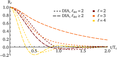
Figure 6: Same as Fig. 3, except that we compare the DIA prediction (Eq. 28) for the ${\ell_{\mathrm{int}}\!=\!2}$ model (small dashes) with the ${\ell_{\mathrm{int}}\!\geq\!2}$ model (large dashes). For even harmonics, the correlations decay faster as one includes more harmonics in the pairwise interaction.

In that figure, the predictions for both models exhibit the same overall behavior, though they differ in their respective correlation times. Indeed, for even harmonics, the model ${\ell_{\mathrm{int}}\!\geq\!2}$ decorrelates faster. Following eq. (15) of Fouvry et al. (2019), we argue that this is because the typical correlation time of a given (even) harmonic is inversely proportional to the sum ${\sum_{\ell_{\mathrm{int}}}\!\!\mathcal{J}^{2}_{\ell_{\mathrm{int}}}}$ (see Fouvry et al., 2019). As a result, the sharper the interaction potential, the faster the decorrelation for the even harmonics. These even harmonics are the sole driver of the dynamics of particles, see after Eq. (30).

Appendix G Higher-order approximation?

Here, we provide the next-order analytical and numerical resolution of Eq. (29). Injecting Eq. (29) into the definition from Eq. (22), we obtain

$$\Sigma_{\mathbf{1}\mathbf{1}^{\prime}}{} =\tfrac{1}{2}\,\gamma_{\mathbf{1}\mathbf{2}\mathbf{3}}\,G_{\mathbf{2}\mathbf{2}^{\prime}}\,G_{\mathbf{3}\mathbf{3}^{\prime}}\,\gamma_{\mathbf{1}^{\prime}\mathbf{2}^{\prime}\mathbf{3}^{\prime}}$$ (93)

$$+\tfrac{1}{2}\,\gamma_{\mathbf{1}\mathbf{2}\mathbf{3}}\,G_{\mathbf{2}\mathbf{2}^{\prime}}\,G_{\mathbf{3}\mathbf{3}^{\prime}}\,\gamma_{\mathbf{1}^{\prime}\mathbf{4}\mathbf{5}}G_{\mathbf{4}\mathbf{4}^{\prime}}\gamma_{\mathbf{2}^{\prime}\mathbf{4}^{\prime}\mathbf{6}}G_{\mathbf{5}\mathbf{5}^{\prime}}\,G_{\mathbf{6}\mathbf{6}^{\prime}}\,\gamma_{\mathbf{3}^{\prime}\mathbf{5}^{\prime}\mathbf{6}^{\prime}}.$$

We now inject Eq. (93) into Eqs. (24a) and (24b), and assume stationarity and isotropy as in Eq. (26). In that case, we recover that the FDT also holds: this is once again a reassuring self-consistency check. After lengthy manipulations, the prediction for the isotropic response function, $R_{\ell}$, in a single population system becomes

$$\frac{\partial R_{\ell_{1}}(t_{0})}{\partial t_{0}}={} -\frac{1}{2\ell_{1}+1}C_{0}\sum_{\ell_{2},\ell_{3}}[\mathcal{J}_{\ell_{2}}\!\!-\!\!\mathcal{J}_{\ell_{3}}][\mathcal{J}_{\ell_{2}}\!\!-\!\!\mathcal{J}_{\ell_{1}}](E^{L}_{\ell_{1}\ell_{2}\ell_{3}})^{2}\!\!\int^{t_{0}}_{0}\!\!\mathrm{d}t\,R_{\ell_{1}}(t)R_{\ell_{2}}(t_{0}\!\!-\!\!t)R_{\ell_{3}}(t_{0}\!\!-\!\!t)$$ (94)

$$+\frac{1}{2\ell_{1}+1}C_{0}^{2}\sum_{\mathclap{\begin{subarray}{c}\ell_{2},\ell_{3}\\ \ell_{4},\ell_{5},\ell_{6}\end{subarray}}}\,[\mathcal{J}_{\ell_{1}}\!\!-\!\!\mathcal{J}_{\ell_{5}}][\mathcal{J}_{\ell_{2}}\!\!-\!\!\mathcal{J}_{\ell_{3}}]\,E^{L}_{\ell_{1}\ell_{2}\ell_{3}}\,E^{L}_{\ell_{1}\ell_{5}\ell_{6}}\,E^{L}_{\ell_{4}\ell_{2}\ell_{6}}\,E^{L}_{\ell_{4}\ell_{5}\ell_{3}}\,W^{\ell_{1}\,\ell_{2}\,\ell_{3}}_{\ell_{4}\,\ell_{5}\,\ell_{6}}$$

$$\times\!\!\int^{t_{0}}_{0}\!\!\mathrm{d}t_{1}\!\!\int^{t_{0}}_{0}\!\!\mathrm{d}t_{2}\!\!\int^{t_{0}}_{0}\!\!\mathrm{d}t_{3}\,R_{\ell_{1}}(t_{3})\,R_{\ell_{2}}(t_{0}\!\!-\!\!t_{2})\,R_{\ell_{3}}(t_{0}\!\!-\!\!t_{1})\,R_{\ell_{4}}(t_{1}\!\!-\!\!t_{2})\,R_{\ell_{5}}(t_{1}\!\!-\!\!t_{3})\,R_{\ell_{6}}(t_{2}\!\!-\!\!t_{3})\,$$

$$\times\!\!\bigg{\{}\!\![\mathcal{J}_{\ell_{5}}\!\!-\!\!\mathcal{J}_{\ell_{4}}][\mathcal{J}_{\ell_{4}}\!\!-\!\!\mathcal{J}_{\ell_{6}}]\,\Theta(t_{0}\!\!-\!\!t_{1})\Theta(t_{0}\!\!-\!\!t_{2})\Theta(t_{2}\!\!-\!\!t_{3})+[\mathcal{J}_{\ell_{4}}\!\!-\!\!\mathcal{J}_{\ell_{3}}][\mathcal{J}_{\ell_{4}}\!\!-\!\!\mathcal{J}_{\ell_{6}}]\,\Theta(t_{0}\!\!-\!\!t_{2})\Theta(t_{2}\!\!-\!\!t_{3})\Theta(t_{3}\!\!-\!\!t_{1})$$

$$+[\mathcal{J}_{\ell_{5}}\!\!-\!\!\mathcal{J}_{\ell_{4}}][\mathcal{J}_{\ell_{6}}\!\!-\!\!\mathcal{J}_{\ell_{2}}]\,\Theta(t_{0}\!\!-\!\!t_{1})\Theta(t_{1}\!\!-\!\!t_{2})\Theta(t_{2}\!\!-\!\!t_{3})+[\mathcal{J}_{\ell_{4}}\!\!-\!\!\mathcal{J}_{\ell_{6}}][\mathcal{J}_{\ell_{3}}\!\!-\!\!\mathcal{J}_{\ell_{5}}]\,\Theta(t_{0}\!\!-\!\!t_{2})\Theta(t_{2}\!\!-\!\!t_{3})\Theta(t_{2}\!\!-\!\!t_{1})\!\!\bigg{\}}.$$

The first term on the rhs is exactly Eq. (28). Here, $\Theta$ is the usual Heaviside function and the coefficients $W^{\ell_{1}\,\ell_{2}\,\ell_{3}}_{\ell_{4}\,\ell_{5}\,\ell_{6}}$ are given by Eq. (41). The numerical solution of Eq. (94) is illustrated in Fig. 7, in the case of the quadrupolar ${\ell_{\mathrm{int}}\!=\!2}$ interaction model.

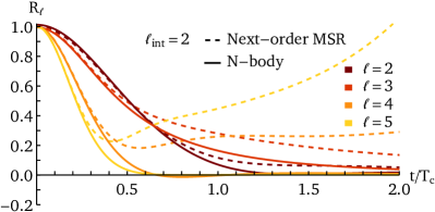
Figure 7: Same as Fig. 3, but for the (naive) higher-order prediction (Eq. 94, dashed lines). On short timescales, the higher-order prediction agrees with the measurements. However, the prediction diverges on longer timescales, and the divergence worsens as the scale becomes smaller.

In Fig. 7, we find that the higher-order prediction from Eq. (94) severely diverges at late times. And, that this divergence worsens as one considers larger $\ell$, i.e. smaller angular scales.

As discussed in Section IV.4, the divergence observed in Fig. 7 originates from the (incorrect) assumption that the expansion of the dressed vertex, $\Gamma$, in terms of the bare vertex, $\gamma$, converges. A brief discussion on a more promising approach to derive the higher-order prediction is mentioned in Section IV.4. This will be the focus of future work.

References

• Kormendy and Ho (2013) J. Kormendy and L. C. Ho, ARA&A 51, 511 (2013).
• Ghez et al. (2008) A. M. Ghez et al., ApJ 689, 1044 (2008).
• Gillessen et al. (2017) S. Gillessen et al., ApJ 837, 30 (2017).
• Paumard et al. (2006) T. Paumard et al., ApJ 643, 1011 (2006).
• Murchikova et al. (2019) E. M. Murchikova, E. S. Phinney, A. Pancoast, and R. D. Blandford, Nature 570, 83 (2019).
• GRAVITY Collaboration et al. (2020) GRAVITY Collaboration et al., A&A 636, L5 (2020).
• Event Horizon Telescope Collaboration et al. (2022) Event Horizon Telescope Collaboration et al., ApJL 930, L12 (2022).
• Rauch and Tremaine (1996) K. P. Rauch and S. Tremaine, New Astron. 1, 149 (1996).
• Merritt (2013) D. Merritt, Dynamics and Evolution of Galactic Nuclei (Princeton Univ. Press, 2013).
• Alexander (2017) T. Alexander, ARA&A 55, 17 (2017).
• Gürkan and Hopman (2007) M. A. Gürkan and C. Hopman, MNRAS 379, 1083 (2007).
• Eilon et al. (2009) E. Eilon, G. Kupi, and T. Alexander, ApJ 698, 641 (2009).
• Kocsis and Tremaine (2015) B. Kocsis and S. Tremaine, MNRAS 448, 3265 (2015).
• Kocsis and Tremaine (2011) B. Kocsis and S. Tremaine, MNRAS 412, 187 (2011).
• Hamers et al. (2018) A. S. Hamers, B. Bar-Or, C. Petrovich, and F. Antonini, ApJ 865, 2 (2018).
• Szölgyén and Kocsis (2018) Á. Szölgyén and B. Kocsis, PRL 121, 101101 (2018).
• Nicholson (1992) D. R. Nicholson, Introduction to Plasma Theory (Krieger, 1992).
• Binney and Tremaine (2008) J. Binney and S. Tremaine, Galactic Dynamics: Second Edition (Princeton Univ. Press, 2008).
• Campa et al. (2014) A. Campa, T. Dauxois, D. Fanelli, and S. Ruffo, Physics of Long-Range Interacting Systems (Oxford Univ. Press, 2014).
• Gupta and Mukamel (2011) S. Gupta and D. Mukamel, J. Stat. Mech. 2011, 03015 (2011).
• Maier and Saupe (1958) W. Maier and A. Saupe, Z. Nat. A. 13, 564 (1958).
• Roupas et al. (2017) Z. Roupas, B. Kocsis, and S. Tremaine, ApJ 842, 90 (2017).
• Roupas (2020) Z. Roupas, J. Phys. A 53, 045002 (2020).
• Taylor and McNamara (1971) J. B. Taylor and B. McNamara, Phys. Fluids 14, 1492 (1971).
• Chavanis et al. (1996) P.-H. Chavanis, J. Sommeria, and R. Robert, ApJ 471, 385 (1996).
• Garcìa-Ojalvo and Sancho (1999) J. Garcìa-Ojalvo and J. M. Sancho, Noise in Spatially Extended Systems (Springer, 1999).
• Krommes (2002) J. A. Krommes, Phys. Rep. 360, 1 (2002).
• Zhou (2021) Y. Zhou, Phys. Rep. 935, 1 (2021).
• Kraichnan (1959a) R. H. Kraichnan, J. Fluid Mech. 5, 497 (1959a).
• Martin et al. (1973) P. C. Martin, E. D. Siggia, and H. A. Rose, Phys. Rev. A 8, 423 (1973).
• Fouvry et al. (2019) J.-B. Fouvry, B. Bar-Or, and P.-H. Chavanis, ApJ 883, 161 (2019).
• Kadomtsev (1965) B. Kadomtsev, Plasma Turbulence (Academic Press, 1965).
• Frisch and Kolmogorov (1995) U. Frisch and A. Kolmogorov, Turbulence: The Legacy of A. N. Kolmogorov (Cambridge Univ. Press, 1995).
• Bernardeau et al. (2002) F. Bernardeau, S. Colombi, E. Gaztañaga, and R. Scoccimarro, Phys. Rep. 367, 1 (2002).
• Lancaster and Blundell (2014) T. Lancaster and S. Blundell, Quantum Field Theory for the Gifted Amateur (OUP Oxford, 2014).
• Peskin and Schroeder (2018) M. E. Peskin and D. V. Schroeder, An Introduction To Quantum Field Theory (CRC Press, 2018).
• Rose (1985) H. A. Rose, Physica D 14, 216 (1985).
• Kraichnan (1958) R. H. Kraichnan, Phys. Rev. 109, 1407 (1958).
• Ottaviani (1990) M. Ottaviani, Phys. Lett. A 143, 325 (1990).
• Kraichnan (1959b) R. H. Kraichnan, Phys. Rev. 113, 1181 (1959b).
• Kraichnan (1961) R. H. Kraichnan, J. Math. Phys. 2, 124 (1961).
• Berera et al. (2013) A. Berera, M. Salewski, and W. D. McComb, Phys. Rev. E 87, 013007 (2013).
• Krommes (1984) J. A. Krommes, in Basic Plasma Physics, Volume 1 (1984), p. 183.
• Fukuda et al. (1995) R. Fukuda et al., Prog. Theor. Phys. 121, 1 (1995).
• Cornwall et al. (1974) J. M. Cornwall, R. Jackiw, and E. Tomboulis, Phys. Rev. D 10, 2428 (1974).
• Berges (2004) J. Berges, Phys. Rev. D 70, 105010 (2004).
• Carrington and Guo (2011) M. E. Carrington and Y. Guo, Phys. Rev. D 83, 016006 (2011).
• Zhou (2010) Y. Zhou, Phys. Rep. 488, 1 (2010).
• Delamotte (2012) B. Delamotte, in Lecture Notes in Physics (Springer, 2012), vol. 852, p. 49.
• Dupuis et al. (2021) N. Dupuis et al., Phys. Rep. 910, 1 (2021).
• Tarpin et al. (2019) M. Tarpin et al., J. Phys. A 52, 085501 (2019).
• Touma et al. (2019) J. Touma, S. Tremaine, and M. Kazandjian, PRL 123, 021103 (2019).
• Gruzinov et al. (2020) A. Gruzinov, Y. Levin, and J. Zhu, ApJ 905, 11 (2020).
• Magnan et al. (2022) N. Magnan et al., MNRAS 514, 3452 (2022).
• Máthé et al. (2023) G. Máthé, Á. Szölgyén, and B. Kocsis, MNRAS 520, 2204 (2023).
• Takács and Kocsis (2018) Á. Takács and B. Kocsis, ApJ 856, 113 (2018).
• Fragione and Loeb (2022) G. Fragione and A. Loeb, ApJL 932, L17 (2022).
• GRAVITY Collaboration et al. (2023) GRAVITY Collaboration et al., A&A 672, A63 (2023).
• Will et al. (2023) C. M. Will et al., ApJ 959, 58 (2023).
• Ginat et al. (2023) Y. B. Ginat, T. Panamarev, B. Kocsis, and H. B. Perets, MNRAS 525, 4202 (2023).
• Giral Martínez et al. (2020) J. Giral Martínez, J.-B. Fouvry, and C. Pichon, MNRAS 499, 2714 (2020).
• Bartko et al. (2009) H. Bartko et al., ApJ 697, 1741 (2009).
• Lu et al. (2009) J. R. Lu et al., ApJ 690, 1463 (2009).
• Yelda et al. (2014) S. Yelda et al., ApJ 783, 131 (2014).
• von Fellenberg et al. (2022) S. D. von Fellenberg et al., ApJL 932, L6 (2022).
• Panamarev and Kocsis (2022) T. Panamarev and B. Kocsis, MNRAS 517, 6205 (2022).
• Fouvry et al. (2023) J.-B. Fouvry, M. J. Bustamante-Rosell, and A. Zimmerman, MNRAS 526, 1471 (2023).
• Varshalovich et al. (1988) D. A. Varshalovich et al., Quantum Theory of Angular Momentum (World Scientific, 1988).
• Binney and Skinner (2013) J. Binney and D. Skinner, The Physics of Quantum Mechanics (OUP Oxford, 2013).
• Fouvry et al. (2022) J.-B. Fouvry, W. Dehnen, S. Tremaine, and B. Bar-Or, ApJ 931, 8 (2022).
• (71) https://github.com/sfloresmo/VRR_DIA.