Task-splitting in home healthcare routing and scheduling

Abstract

This paper introduces the concept of task-splitting into home healthcare (HHC) routing and scheduling. It focuses on the design of routes and timetables for caregivers providing services at patients’ homes. Task-splitting is the division of a (lengthy) patient visit into separate visits that can be performed by different caregivers at different times. The resulting split parts may have reduced caregiver qualification requirements, relaxed visiting time windows, or a shorter/longer combined duration. However, additional temporal dependencies can arise between them. To incorporate task-splitting decisions into the planning process, we introduce two different mixed integer linear programming formulations, a Miller-Tucker-Zemlin and a time-indexed variant. These formulations aim to minimize operational costs while simultaneously deciding which visits to split and imposing a potentially wide range of temporal dependencies. We also propose pre-processing routines for the time-indexed formulation and two heuristic procedures. These methods are embedded into the branch-and-bound approach as primal and improvement heuristics. The results of our computational study demonstrate the additional computational difficulty introduced by task-splitting and the associated additional synchronization, and the usefulness of the proposed heuristic procedures. From a planning perspective, our results indicate that introducing task-splitting reduces staff requirements, decreases HHC operational costs, and allows caregivers to spend relatively more time on tasks aligned with their qualifications. Moreover, we observe that the potential of task-splitting is not specific to the chosen planning objective; it can also be beneficial when minimizing travel time instead.

Keywords: OR in health services, Home health care, Task-splitting, Temporal dependencies, Integer programming

1 Introduction

In industrialized countries, healthcare providers are confronted with the consequences of an aging population, which drives an increase in the demand for healthcare services. One of the sectors particularly affected by this is home healthcare (HHC), which will play an increasingly prominent role in making healthcare affordable. In the United Kingdom, for instance, this translates into a projected compound annual growth rate for the sector of 9.1% until 2030 (GVR, 2023). HHC involves caregivers traveling to patients’ homes to provide various services, including assistance with taking medication, administering injections, wound care, or showering. The benefits of HHC are twofold. Firstly, people prefer to age at home (Wiles et al., 2011) as it allows them to retain their autonomy. Secondly, it is a cost-effective alternative to traditional hospital care. However, the supply of HHC services is already under pressure due to staff shortages, so meeting the growing demand from an aging population presents a significant challenge.

Driven by the social relevance of affordable and reliable HHC, home healthcare planning has received significant research attention in recent years. The focus has been on the design of efficient routes and corresponding schedules for caregivers, formally known as Home Healthcare Routing and Scheduling Problems (HHCRSPs). These planning problems typically include issues such as: i) caregivers having specific capacities and work preferences, ii) patient visits having service and time constraints, and iii) the need to synchronize multiple visits for the same patient. Given the complexity of these planning processes, further optimization of caregiver schedules is one element that HHC providers can do to improve caregiver allocation.

The diverse national and regulatory settings have led to the emergence of numerous variants of the HHCRSP. Overviews of the wide range of modeling and solution approaches utilized are provided by Euchi et al. (2022); Di Mascolo et al. (2021); Fikar and Hirsch (2017). Most research relates to the daily planning of care, with time windows indicating when care can be provided. Other commonly considered characteristics are the required qualifications of visiting caregivers, the permitted working hours, and the legislative rules for caregivers.

Temporal restrictions between visits further complicate the already challenging task of solving the basic types of HHCRSPs. They create interdependence between caregiver routes and schedules, resulting in complex planning challenges (Soares et al., 2024; Drexl, 2012). For example, strict synchronization occurs if two caregivers are required for a certain task, such as lifting a disabled person. Precedence refers to a certain minimum and/or maximum amount of time needed between two visits (e.g., medication before or after dinner). Disjunctive requirements imply that two tasks must be executed on non-overlapping moments in time (e.g., assistance with bathing and a medical treatment). These temporal dependencies are more generally referred to as synchronization and may also arise, for example, when a patient’s care tasks are split among multiple visits. Despite the fact that synchronization restrictions can be required for approximately 20% of the patient visits (Polnik et al., 2020), most papers ignore some or all observed synchronization types (Clapper et al., 2023; Xiang et al., 2023; Yin et al., 2023; Pahlevani et al., 2022), which reduces the related modeling complexity. However, there is a growing interest in the handling of synchronization restrictions, which is supported by the development of a wide variety of heuristic approaches. These heuristics primarily address variants of HHCRSPs that permit the simultaneously execution of tasks (Dai et al., 2023; Masmoudi et al., 2023; Bazirha et al., 2023; Erdem et al., 2022; Liu et al., 2021; Euchi et al., 2020; Decerle et al., 2019; Bredström and Rönnqvist, 2008; Eveborn et al., 2006). Other temporal restrictions are also studied (Oladzad-Abbasabady et al., 2023; Shahnejat-Bushehri et al., 2021; Yadav and Tanksale, 2022; Frifita and Masmoudi, 2020; Ait Haddadene et al., 2019; Mankowska et al., 2014).

Contrary to the variety of heuristic approaches, only a few exact solution methods for HHCRSPs have been proposed to handle synchronization requirements. Rasmussen et al. (2012) developed a Branch-and-Price (BP) approach for an HHCRSP with strict synchronization and precedence. Their BP utilizes a set partition model and enforces synchronization via time window branching. Mankowska (2016) proposes a combinatorial Benders approach for solving an HHCRSP with strict synchronization and precedence. Their master problem fixes the caregiver routes, and the continuous subproblem determines the timing of the route (e.g., temporal dependencies). Qiu et al. (2022) describe a Branch-and-Price-and-Cut (BPC) for an HHCRSP where the starting times of synchronized visits must be within a certain range of each other. During their BPC, they create initial caregiver routes with Adaptive Large Neighborhood Search and solve the pricing problem with a specially designed labeling algorithm. Hashemi Doulabi et al. (2020) investigate an HHCRSP that includes strict synchronization and stochastic travel and service times. They solve it with an L-shaped and a Branch-and-Cut algorithm, using valid inequalities for subtours, capacity constraints, and no overlap constraints. Despite the ability of exact solution methods to provide optimal solutions, their practical use is limited by high computational needs.

A broader perspective reveals that many HHCRSPs can be classified as specific types of vehicle routing problems (VRPs) with synchronization. Such problems have been addressed by Shi et al. (2020); Liu et al. (2019); Parragh and Doerner (2018); Afifi et al. (2016). While the majority of research on exact solution methods for VRPs with synchronization focuses on a homogeneous fleet (Dohn et al., 2011; Bredström and Rönnqvist, 2007), there are also articles considering heterogeneous sets of vehicles. For instance, Dohn et al. (2009); Luo et al. (2016) developed BP(C) algorithms for set partition formulations, securing synchronization through time window branching.

In addition to HHCRSPs that consider caregivers who travel independently, settings are studied in which teams of two caregivers travel together. Synchronization can then be used to allow the splitting of some caregiver teams traveling together. In de Aguiar et al. (2023); Nozir et al. (2020), patient visits requiring a team of two caregivers are allowed to be also served by two simultaneous visits of caregivers traveling independently. The results indicate that this can result in less staff being required and higher planning efficiency, suggesting the potential of splitting resources.

In practice, HHC providers have already explored various methods for organizing their work more efficiently. For instance, some organizations in the Netherlands switched from a hierarchical top-down structure to a bottom-up team-based structure, enabling caregivers to work in self-managing teams (Renkema et al., 2018). Another approach consists of differentiating tasks within a visit and assigning them to caregivers with different skill levels at different moments in time. This approach enables caregivers with specific medical skills to perform fewer tasks outside their area of expertise, which can help to reduce specific staff shortages. However, a formal investigation of the decision-making process regarding the division of tasks within the context of a patient visit has yet to be conducted. As a result, no tools are currently available to support such decisions. Motivated by contacts within the healthcare sector, this paper formally investigates whether task-splitting can contribute to enhanced caregiver planning in the home healthcare sector.

Task-splitting is the division of a (potentially inefficient) lengthy patient visit into multiple, shorter visits. This introduces additional scheduling flexibility for HHC providers. To the best of our knowledge, this is the first paper to incorporate the decision of whether a visit should be split into the planning process. The advantages of task-splitting emerge in a number of ways. First, it can result in a better use of the available staff, as one of the split parts may require lower qualifications from caregivers (e.g., bathing could be performed by caregivers with a different skill set). Second, it allows the split parts to be performed at different times, thus reducing the peak demand (e.g., performing medical treatment at a later point in time). Third, it can result in improved alignment between patient needs and caregivers, as caregiver qualifications can be indicated for both split parts. Lastly, task-splitting can lead to efficiency gains, for example, by eliminating mandatory waits between two tasks. Caution should be taken when deciding whether to split tasks. For instance, patients may not wish to have numerous different visiting caregivers or be forced to remain at home all day. Temporal restrictions between the execution of the different split parts must also be taken into account, which complicates the planning problem. For example, tasks requiring contact with the patient, such as bathing and medical care, cannot be performed simultaneously. This type of non-overlapping temporal restriction is another element that has not been addressed in the current exact solution methods for HHCRSPs. The potential of task-splitting extends beyond the scope of HHC. It could also occur in care homes or hospitals, for example. Therefore, the relevance of this research is broader than home care; it is also of interest to related (healthcare) settings that face similar (future) staffing challenges.

The objective of this article is to provide support for the incorporation of task-splitting into home healthcare planning and to explore its impact on HHC providers and related settings. The main contributions of this article are:

• We propose the first variant of the HHCRSP that incorporates task-splitting possibilities, a wide range of synchronization restrictions, and a natural type of operational costs.

• We develop two integer linear programming formulations incorporating task-splitting decisions: a Miller-Tucker-Zemlin formulation and a time-indexed formulation.

• We introduce pre-processing techniques and two heuristic procedures to improve the computational performance of the resulting solution algorithm.

• We explore the computational challenges and managerial benefits of task-splitting in HHC.

The remainder of this paper is organized as follows. Section 2 defines the newly introduced problem variant. In Section 3, we present a Miller-Tucker-Zemlin and a time-indexed integer linear program (ILP) formulation. Section 4 discusses some pre-processing techniques and proposes two types of heuristic procedures to enrich an integer linear programming solver. Section 5 describes the generation of benchmark instances. Section 6 presents the results of our computational study, which incorporates an analysis of the computational characteristics and an exploration of the effect of task-splitting on caregiver allocations in various scenarios. Finally, we summarize the findings and outline potential directions for further research in Section 7.

2 Problem definition

This section formally introduces the Home Healthcare Routing and Scheduling Problem with Task-Splitting (HHCRSP-TS), which aims to design optimal routes and timetables for caregivers that provide a service at patients’ homes. The problem considers a set of caregivers, denoted by $C$, who perform a set of original patient visits $V^{\mathrm{o}}=\{1,\dots,n\}$ within a planning horizon $[0,T_{\mathrm{max}}]$. Each caregiver $k\in C$ is associated with a qualification type $q_{k}$ from the set of qualification types $Q$. Each patient visit $v\in V^{\mathrm{o}}$ is associated with a set of qualifications $Q_{v}\subseteq Q$ that specify which types of caregivers can perform visit $v$, the visit duration $d_{v}$, $0<d_{v}\leq T_{\mathrm{max}}$, and a time window $[\alpha_{v},\beta_{v}]$, $0\leq\alpha_{v}<\beta_{v}\leq T_{\mathrm{max}}-d_{v}$, during which visit $v$ must start.

The subset $S\subseteq V^{\mathrm{o}}$ contains visits that are comprised of multiple tasks that can be split into two separate parts. Each splittable visit $v\in S$ can either be performed as a whole or replaced by two split visits $v_{p}$, $p\in\{1,2\}$ with qualification types $Q_{v_{p}}\subseteq Q$, durations $d_{v_{p}}$, $0<d_{v_{p}}\leq T_{\mathrm{max}}$, and time windows $[\alpha_{v_{p}},\beta_{v_{p}}]$, $0\leq\alpha_{v_{p}}<\beta_{v_{p}}\leq T_{\mathrm{max}}-d_{v_{p}}$. When combined with the unsplit visits, this generates the set of potential patient visits $V=V^{\mathrm{o}}\cup\{v_{p}:v\in S,\;p\in\{1,2\}\}$. When the splittable visit $v\in S$ is split into two separate parts, one of the split parts $v_{p}$, $p\in\{1,2\}$ may be performed by a wider range of caregivers (i.e., $Q_{v}\subseteq Q_{v_{p}}$). Moreover, the combined duration of the split parts may differ from that of the original visit $v$ due to efficiency gains or losses (i.e., $d_{v}\neq d_{v_{1}}+d_{v_{2}}$). It may also be possible to perform the split parts at different points in time (i.e., $[\alpha_{v_{p}},\beta_{v_{p}}]\neq[\alpha_{v},\beta_{v}]$).

Set $D\subseteq V^{2}$ encompasses all pairs of visits with temporal dependencies, such as precedence requirements, overlapping or non-overlapping visiting times, or a simultaneous start of the visits. The HHCRSP-TS considers a generic set of synchronization requirements by associating parameters $\delta_{uv}^{\mathrm{min}}$ and $\delta_{uv}^{\mathrm{max}}$ to each ordered pair $(u,v)$ of visits $\{u,v\}\in D$ with temporal dependencies. This yields four parameters for each such pair of visits. Thus, $\delta_{uv}^{\mathrm{min}}$ and $\delta_{uv}^{\mathrm{max}}$ indicate the permitted minimum and maximum difference in the starting times of visits $u$ and $v$ if visit $u$ starts before or simultaneously with visit $v$. This means that starting time $t\in[\alpha_{u},\beta_{u}]$ imposes the start of visit $v$ within the time window $[t+\delta_{uv}^{\mathrm{min}},t+\delta_{uv}^{\mathrm{max}}]$. Table 1 summarizes various synchronization types and their corresponding parameter values.

Table 1: Synchronization types that can be considered in the HHCRSP-TS and corresponding parameter values. Here, $u\preceq v$ indicates that visit $u$ must start before visit $v$, while $\Delta_{\mathrm{min}}$ and $\Delta_{\mathrm{max}}$ specify the minimum and maximum permitted differences of their starting times.

synchronization type		parameter values
ordering	temporal aspect	$\delta_{uv}^{\mathrm{min}}$	$\delta_{uv}^{\mathrm{max}}$	$\delta_{vu}^{\mathrm{min}}$	$\delta_{vu}^{\mathrm{max}}$
-	strict synchronization (simultaneous start)	0	0	0	0
-	limit difference of start (min. $\Delta_{\mathrm{min}}$, max. $\Delta_{\mathrm{max}}$)	$\Delta_{\mathrm{min}}$	$\Delta_{\mathrm{max}}$	$\Delta_{\mathrm{min}}$	$\Delta_{\mathrm{max}}$
-	visits must overlap	0	$d_{u}$	0	$d_{v}$
-	visits must not overlap	$d_{u}$	$T_{\mathrm{max}}$	$d_{v}$	$T_{\mathrm{max}}$
$u\preceq v$	visit must be completed	$d_{u}$	$T_{\mathrm{max}}$	$T_{\mathrm{max}}$	$T_{\mathrm{max}}$
$v\preceq u$	visit must be completed	$T_{\mathrm{max}}$	$T_{\mathrm{max}}$	$d_{v}$	$T_{\mathrm{max}}$
$u\preceq v$	limit difference of start (min. $\Delta_{\mathrm{min}}$, max. $\Delta_{\mathrm{max}}$)	$\Delta_{\mathrm{min}}$	$\Delta_{\mathrm{max}}$	$T_{\mathrm{max}}$	$T_{\mathrm{max}}$
$v\preceq u$	limit difference of start (min. $\Delta_{\mathrm{min}}$, max. $\Delta_{\mathrm{max}}$)	$T_{\mathrm{max}}$	$T_{\mathrm{max}}$	$\Delta_{\mathrm{min}}$	$\Delta_{\mathrm{max}}$

Parameter $t_{uv}\geq 0$ indicates the time it takes a caregiver to travel from visit $u\in V$ to visit $v\in V$ while cost parameter $e^{q}\geq 0$ represents the wage (per time unit) of a caregiver with qualification $q\in Q$. The objective of the HHCRSP-TS is to identify a plan with minimal overall costs in which each patient visit is performed by a sufficiently qualified caregiver within the given time window and in which all temporal dependencies are respected. For each splittable visit $v\in S$, either the original visit $v$ or both split visits $v_{p}$, $p\in\{1,2\}$, must be performed. The costs of each plan are equal to the sum of all total working times of all caregivers multiplied by the wage parameter commensurate with each caregiver’s qualification. Thereby, the total working time of a caregiver is defined as the sum of time spent on patient visits, the travel time between visits, and any waiting time possibly required before or after visits in order to meet the time windows of subsequent visits. Let $\mathcal{P}$ denote the set of all feasible plans in the HHCRSP-TS, $t_{\mathrm{start}}^{k}(P)$ denote the starting time of the first visit and $t_{\mathrm{end}}^{k}(P)$ donate the end time of the last visit of caregiver $k\in C$ in plan $P\in\mathcal{P}$. Then, the objective of the HHCRSP-TS is to identify a plan $P^{*}$ that minimizes the total cost, i.e.,

$$P^{*}\in\mathrm{arg\,min}_{P\in\mathcal{S}}\sum_{k\in C}e^{q_{k}}(t_{\mathrm{end}}^{k}(P)-t_{\mathrm{start}}^{k}(P)).$$

An example of the HHCRSP-TS is provided in Figure 1. The example illustrates a situation involving three visits in the early morning and two at the end of the morning. Each house represents an original patient visit. The permitted care initiation times are indicated by the associated time window and the requested care tasks are indicated by icons. Introducing the option to split the tasks of the visit at the bottom house means both tasks no longer have to be performed immediately after each other by the most medically trained type of caregiver. This allows all care requests to be fulfilled with either fewer caregivers (2 instead of 3, bottom left) or with a lower number of working hours (-30 minutes, bottom right). Note that task-splitting results in more work being shifted to the least medically trained caregiver.

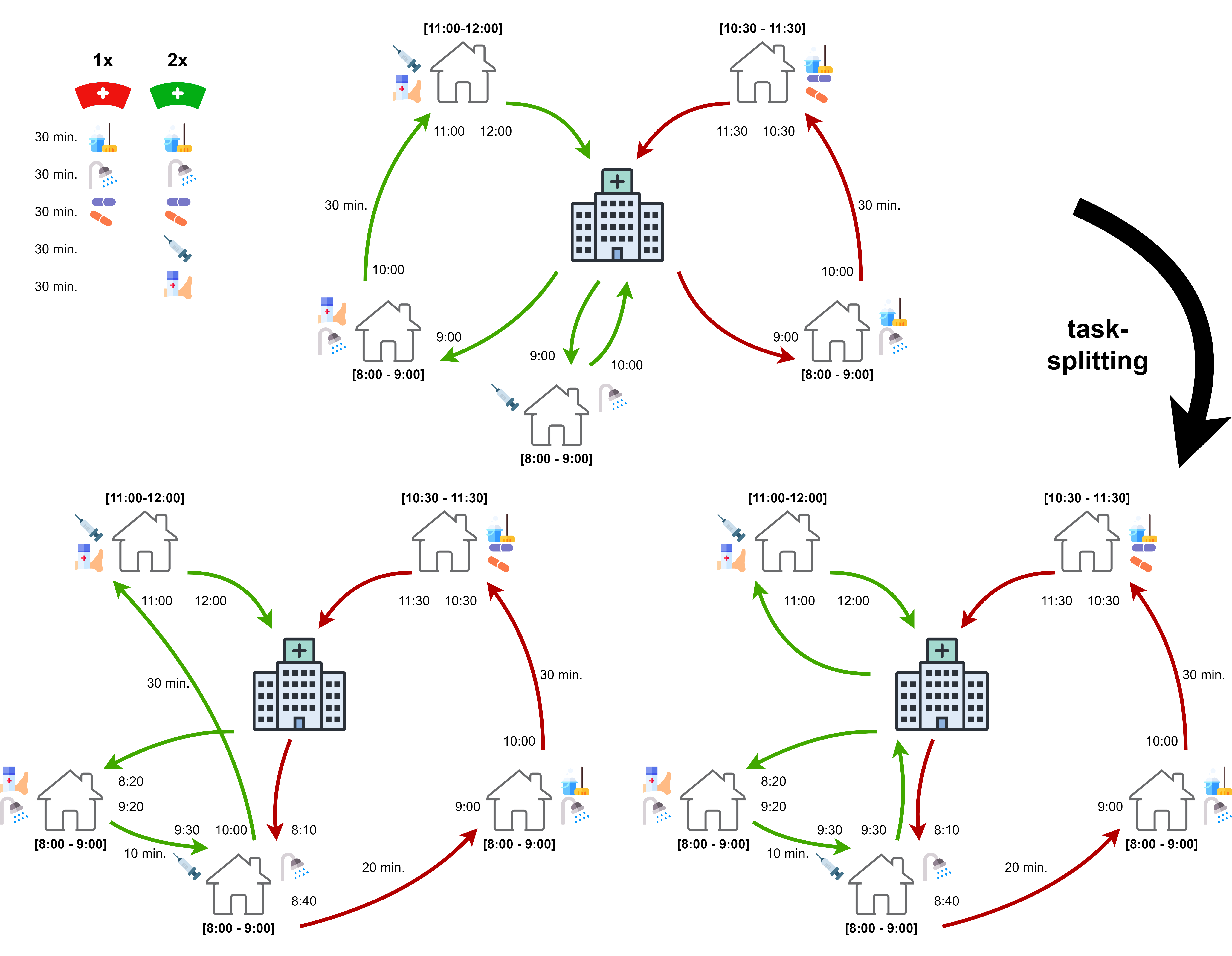
Figure 1: Visualization of an HHCRSP-TS. Each house represents an original visit. The interval next to it represents the time window within which care can be initiated. The icons next to each house represent the required care tasks. Two different types of caregivers are available, and the arcs of their corresponding color represent their routes. The introduction of task-splitting at the bottom visit allows the same collection of care tasks to be performed with fewer caregivers (bottom left) or in fewer working hours (bottom right).

Focusing on total travel time

The HHCRSP-TS includes the wage of the entire working shift of a caregiver in the objective function. In practice, travel time between patients is typically defined as working time (see, for example, the Dutch labor agreement; SOVVT (2023)). To reflect the operational costs of a caregiver for an HHC provider, we incorporate a caregiver’s wage from the start of their first visit until the completion of their last visit. It is important to note that most related research focuses on the total travel time. Waiting times at the patient’s home and differences in caregiver hourly wages are typically ignored. This originates, for example, from a focus on the (reimbursement of) travel expenses (see, e.g., Pahlevani et al. (2022); Liu et al. (2021)). In our computational experiments, we will also consider a variant of the HHCRSP-TS, denoted as HHCRSP-TS-TT, whose objective is to minimize the total travel time of all caregivers (thus neglecting visit time, waiting times, and wage differences).

Assumptions and notation

In the remainder of this paper, we assume that the same caregiver cannot perform two split parts of a splittable visit consecutively, as this would correspond to an unsplit visit. We also assume that the travel time between patient visits satisfies the triangle inequality. Moreover, we observe that the objective is indifferent to the location of the potential waiting time between two consecutive visits, whether it occurs at the location of the previous visits, while traveling, or at the next visit. Therefore, without loss of generality, we assume that caregivers always travel to their next patient before waiting. To simplify the notation, we add the artificial visits $0$ and $n+1$ to model the start and end of a workday, respectively, resulting in the total set of visits $N=V\cup\{0,n+1\}$. All travel times from or to these artificial nodes are assumed to be equal to zero, i.e., $t_{0v}=0$, $\forall v\in N\setminus\{0\}$ and $t_{v,n+1}=0$, $\forall v\in N\setminus\{n+1\}$. We also assign to both artificial nodes a time window $[0,T_{\mathrm{max}}]$ that can be visited by caregivers of all qualifications, i.e., $\alpha_{0}=\alpha_{n+1}=0$, $\beta_{0}=\beta_{n+1}=T_{\mathrm{max}}$, and $Q_{0}=Q_{n+1}=Q$. Throughout this paper, we use the following notation. The set of all caregivers with qualification $q\in Q$ will be denoted as $C_{q}=\{k\in C:q_{k}=q\}$, $C_{q}\subseteq C$. For a graph $G^{\prime}=(V^{\prime},A^{\prime})$ and a set of nodes $W\subset V^{\prime}$, we use $\delta^{+}(W)=\{(u,v)\in A^{\prime}\mid u\in W,v\notin W\}$. For simplicity, we write $\delta^{+}(u)$ instead of $\delta^{+}(\{u\})$ for node sets of size one. Finally, for a set of variables $Y$ defined on set $U$ and subset $U^{\prime}\subseteq U$, we use the notation $Y(U^{\prime})=\sum_{u\in U^{\prime}}Y_{u}$.

3 Mathematical formulations

This section presents two mixed-integer linear programming formulations for the HHCRSP-TS. The formulation of Section 3.1 uses Miller-Tucker-Zemlin (MTZ) constraints (Miller et al., 1960), while Section 3.2 introduces a time-indexed flow formulation (Picard and Queyranne, 1978).

3.1 Miller-Tucker-Zemlin formulation

The formulation introduced in this section is defined on the graph $G=(N,A)$, whose nodes $N$ correspond to all potential visits and whose arcs $A\subset N\times N$ represent potential travels between them. Arc set $A$ is the disjoint union of starting arcs $A_{\mathrm{start}}=\{(0,v):v\in V\}$, which indicate travel to a patient’s location at the start of a workday, and care arcs $A_{\mathrm{care}}=\{(u,v):u\in V,v\in V\cup\{n+1\},u\neq v,Q_{u}\cap Q_{v}\neq\emptyset,\alpha_{u}+d_{u}+t_{uv}\leq\beta_{v}\}\setminus\{(u,v):\exists w\in S:u,v\in\{w,w_{1},w_{2}\}\}$. Each care arc $(u,v)\in A_{\mathrm{care}}$ represents performing visit $u\in V$ and then traveling to visit $v\in V\cup\{n+1\}$. Please note that care arcs between two visits are only included if they can be performed by a single caregiver in the given order. The latter is only possible if at least one qualification type allows both to be performed and one can arrive at the second visit before its latest starting time. Note also that travels between a splittable visit and its two split visits are excluded, since either the split visits or the original visit are performed, but not both. Similarly, direct travels between two split visits of the same original visit are excluded because the two split visits may not be performed immediately after each other (in this case, the original visit is performed).

Formulation (1) uses the following sets of variables. For each arc $a=(u,v)\in A$ and feasible qualification $q\in Q_{u}\cap Q_{v}$, travel variables $x_{a}^{q}\in\{0,1\}$ indicate whether a caregiver with qualification $q$ travels along arc $(u,v)$, i.e., performs visits $u$ and $v$ immediately after each other. Split variables $s_{v}\in\{0,1\}$ indicate whether a splittable visit $v\in S$ is split (in which case split parts $v_{1}$ and $v_{2}$ must be performed) or not (in which case the original visit $v$ is executed) while variables $y_{v}\in\{0,1\}$ indicate whether visit $v\in V$ is performed or not. Precedence variables $p_{uv}\in\{0,1\}$ are used to model the sequence in which pairs of visits $\{u,v\}\in D$ with temporal dependencies are performed. Thereby, pairs of visits $\{u,v\}\in D$ are considered in an ordered manner such that $u<v$, and $p_{uv}=1$ indicates that visit $u$ starts before or at the same time as visit $v$. Conversely, $p_{uv}=0$ indicates either that visit $v$ starts before or at the same time as visit $u$, or that at least one of these two visits is not performed at all (which can only happen for splittable visits and their split parts). Continuous variables $b_{v}\geq 0$ represent the starting time of the care of visit $v\in V$ and are set to zero for splittable or split visits that are not performed. Additionally, if a visit $v\in V$ is the first visit of a caregiver route of type $q\in Q$, then variable $k_{v}^{q}$ is equal to the starting time of visit $v$. Similarly, if a visit $v\in V$ is the last scheduled visit of a caregiver route with qualification $q\in Q$ then variable $f_{v}^{q}$ is equal to the end time of the visit. If no schedule for a caregiver with qualification $q$ starts (ends) at $v$, variable $k_{v}^{q}$ (variable $f_{v}^{q}$) is equal to zero.

min $$\sum_{v\in V}\sum_{q\in Q_{v}}e^{q}(f^{q}_{v}-k^{q}_{v})$$ (1a)

s.t. $$x^{q}(\delta^{+}(0))\leq|C_{q}| \forall q\in Q$$ (1b)

$$x^{q}(\delta^{+}(v))=x^{q}(\delta^{-}(v)) \forall v\in V,\ q\in Q_{v}$$ (1c)

$$\sum_{q\in Q_{v}}x^{q}(\delta^{+}(v))=y_{v} \forall v\in V$$ (1d)

$$y_{v}=\begin{cases}1&\mbox{if $v\in V^{\mathrm{o}}\setminus S$}\\ 1-s_{v}&\mbox{if $v\in S$}\\ s_{v}&\mbox{ otherwise }\end{cases} \forall v\in V$$ (1e)

$$b_{u}+d_{u}+t_{uv}\sum_{q\in Q_{u}\cap Q_{v}}x^{q}_{uv}\leq b_{v}+(\beta_{u}+d_{u})(1-\sum_{q\in Q_{u}\cap Q_{v}}x^{q}_{uv}) \forall(u,v)\in A,\ u,v\in V$$ (1f)

$$\alpha_{v}y_{v}\leq b_{v}\leq\beta_{v}y_{v} \forall v\in V$$ (1g)

$$b_{v}-\beta_{v}(1-x_{(0,v)}^{q})\leq k_{v}^{q}\leq b_{v} \forall v\in V,\ q\in Q_{v}$$ (1h)

$$k_{v}^{q}\leq(T_{\mathrm{max}}-d_{v})x_{(0,v)}^{q} \forall v\in V,\ q\in Q_{v}$$ (1i)

$$b_{v}+d_{v}-(\beta_{v}+d_{v})(1-x_{(v,n+1)}^{q})\leq f_{v}^{q}\leq b_{v}+d_{v} \forall v\in V,\ q\in Q_{v}$$ (1j)

$$d_{v}x_{(v,n+1)}^{q}\leq f_{v}^{q}\leq T_{\mathrm{max}}x_{(v,n+1)}^{q} \forall v\in V,\ q\in Q_{v}$$ (1k)

$$2p_{uv}\leq y(\{u,v\}) \forall\{u,v\}\in D,u<v$$ (1l)

$$b_{v}-b_{u}\leq\delta^{\mathrm{max}}_{uv}p_{uv}+\beta_{v}(2-y(\{u,v\})) \forall\{u,v\}\in D,u<v$$ (1m)

$$b_{u}-b_{v}\leq\delta^{\mathrm{max}}_{vu}(y_{v}-p_{uv})+\beta_{u}(2-y(\{u,v\})) \forall\{u,v\}\in D,u<v$$ (1n)

$$b_{v}-b_{u}\geq\delta^{\mathrm{min}}_{uv}p_{uv}-\beta_{u}(2-y(\{u,v\}))-\max\{0,\beta_{u}-\alpha_{v}\}(y_{u}-p_{uv}) \forall\{u,v\}\in D,u<v$$ (1o)

$$b_{u}-b_{v}\geq\delta^{\mathrm{min}}_{vu}(y_{v}-p_{uv})-(\beta_{v}+\delta^{\mathrm{min}}_{vu})(2-y(\{u,v\}))$$ (1p)

$$\quad\quad\quad\quad-\max\{0,\beta_{v}-\alpha_{u}\}p_{uv} \forall\{u,v\}\in D,u<v$$ (1q)

$$y_{v}\in\{0,1\} \forall v\in V$$ (1r)

$$x_{uv}^{q}\in\{0,1\} \forall(u,v)\in A,\ q\in Q_{u}\cap Q_{v}$$ (1s)

$$s_{v}\in\{0,1\} \forall v\in S$$ (1t)

$$p_{uv}\in\{0,1\} \forall\{u,v\}\in D,u<v$$ (1u)

$$b_{v}\geq 0 \forall v\in V$$ (1v)

$$k_{v}^{q}\geq 0 \forall v\in V,\ q\in Q_{v}$$ (1w)

$$f_{v}^{q}\geq 0 \forall v\in V,\ q\in Q_{v}$$ (1x)

The objective (1a) minimizes the operational costs for the HHC provider by multiplying the total working time per qualification type by the wage parameter. Constraints (1b) ensure that at most the $|C_{q}|$ available caregivers with qualification type $q\in Q$ can be used. Equations (1c) are flow conservation constraints for caregiver routes. Equations (1d) ensure that an appropriately qualified caregiver arrives at the location of a visit. Constraints (1e) link visit and splitting decisions and ensure that each unsplittable visit is performed. For splittable visit $v\in S$, equations (1e) ensure that either visit $v$ or both of its split parts are executed. Even though visit variables could be easily eliminated using equations (1e), they are retained as they simplify (the explanation of) the synchronization constraints (1l)–(1q). Inequalities (1f) are commonly used MTZ constraints that ensure that the earliest starting time of a patient visit is equal to the end time of the previous visit plus the travel time between these two visits. These constraints also eliminate subtours. Lower and upper bounds on visit starting times are imposed by (1g), which also force the visiting times of visits that are not performed to zero. Together, constraints (1b)–(1g) ensure that all required care is provided by sufficiently qualified caregivers while respecting the time window of each visit.

Constraints (1h)–(1k) ensure the appropriate route starting and finalization times. Therefore, constraints (1h) and (1i) ensure that when a visit $v\in V$ is the first visit of a caregiver route of qualification type $q\in Q_{v}$, variable $k_{v}^{q}$ is equal to the starting time $b_{v}$ of visit $v$ (constraints (1h)), while $k_{v}^{q}$ equals zero otherwise (constraints (1i)). Similarly, constraints (1j) and (1k) ensure that when a visit $v\in V$ is the last visit of a caregiver route of qualification $q\in Q_{v}$, variable $f_{v}^{q}$ is equal to the end time of visit $v$, and equal to zero otherwise.

Constraints (1l)–(1q) ensure that the temporal dependencies for pairs of visits $\{u,v\}\in D$ are met if both visits are performed. Inequalities (1l) ensure that a precedence decision that visit $u\in V$ starts before (or at the same time as) visit $v\in V$ is only possible if both visits are performed. Constraints (1m) and (1n) ensure that, depending on the starting order of $u$ and $v$, the second visit is initiated at most $\delta^{\mathrm{max}}_{uv}$ or $\delta^{\mathrm{max}}_{vu}$ time steps after the first one (if both are performed). These constraints are redundant due to their rightmost terms if (at least) one of the two visits is not performed. Similarly, a bound $\delta^{\mathrm{min}}_{uv}$ or $\delta^{\mathrm{min}}_{vu}$ on the minimum difference between the starting times is imposed by inequalities (1q) and (1o), depending on the temporal sequence of tasks $\{u,v\}\in D$ if both are executed. The two right-most terms on the right-hand sides of these constraints make them redundant if one of the visits is not performed and if the left-hand sides of constraints (1o) or (1q), respectively, correspond to the opposite temporal starting order.

A formulation for the HHCRSP-TS-TT is derived from formulation (1) by replacing the objective function (1a) by $\sum_{(u,v)\in A}\sum_{q\in Q_{u}\cap Q_{v}}t_{uv}x_{(u,v)}^{q}$, which sums up the travel time of all travels performed, and by removing variables $k^{q}_{v}$ and $f^{q}_{v}$, $\forall v\in V$, $\forall q\in Q_{v}$, as well as constraints (1h)–(1k).

3.2 Time-indexed flow formulation

The time-indexed formulation introduced in this section is defined on a time-indexed graph $\mathcal{G}=(\mathcal{N},\mathcal{A})$ and assumes that all time-related input parameters (travel times, time windows, etc.) are integer numbers. To this end, we observe that every instance with rational values can be easily transformed into one containing integer numbers by simple rescaling. The node set $\mathcal{N}=\{0\}\cup\mathcal{N}(V)\cup\{n+1\}$ of graph $\mathcal{G}$ consists of start node $0$, end node $n+1$, and the set of nodes $\mathcal{N}(V)=\cup_{v\in V}\mathcal{N}(v)$ where $\mathcal{N}(v)=\{v^{t}\mid t\in\{\alpha_{v},\dots,\beta_{v}\}\}$ contains one node $v^{t}$ for each possible initiation time $t$ of visit $v$. Inspired by Fink et al. (2019), we classify the set of arcs $\mathcal{A}=\mathcal{A}_{\mathrm{start}}\cup\mathcal{A}_{\mathrm{care}}\cup\mathcal{A}_{\mathrm{wait}}$ into starting arcs $\mathcal{A}_{\mathrm{start}}=\{(0,v^{t})\mid v^{t}\in\mathcal{N}(V)\}$ representing the start of a caregivers workday, waiting arcs $\mathcal{A}_{\mathrm{wait}}=\{(v^{t},v^{t+1})\mid v^{t},v^{t+1}\in\mathcal{N}(V)\}$ representing one time-unit of waiting at a patient’s home, and care arcs $\mathcal{A}_{\mathrm{care}}=\{(u^{t},v^{\ell}):u^{t},v^{\ell}\in\mathcal{N}(V),(u,v)\in A,Q_{u}\cap Q_{v}\neq\emptyset,\ell=\max\{t+d_{u}+t_{uv},\alpha_{v}\}\cup\{(v^{t},n+1\mid u^{t}\in\mathcal{N}(V)\}$ $\setminus\{(u^{t},v^{\ell})\in\mathcal{N}(V)^{2}:\exists w\in S:u,v\in\{\{w,w_{1},w_{2}\}\}$. Please note that waiting at a patient’s home may be required even if a caregiver arrives within that patient’s time window due to temporal restrictions with the initiation of other visits. A care arc $(u^{t},v^{\ell})$ with $u,v\in V$ represents the start of visit $u$ at time $t$ followed by a travel to visit $v\in V\setminus\{u\}$ where the caregiver arrives at time $t+d_{u}+t_{uv}$. Thus, arc $(u^{t},v^{\ell})$ where $\ell=\max\{t+d_{u}+t_{uv},\alpha_{v}\}$ includes waiting time possibly required at visit $v$ if a caregiver arrives before the earliest time $\alpha_{v}$ the care at $v$ can start. These care arcs only exist between visit pairs that have a common required qualification type, since a single caregiver must be capable of performing both visits. A care arc $(u^{t},n+1)$ indicates that visit $u$ initiated at time $t$ is the last visit of a caregiver’s schedule.

Due to the time-indexed nature of graph $\mathcal{G}$, the total working time corresponding to each of its arcs is fixed and we can associate each arc $a\in\mathcal{A}$ with costs

$$c_{a}=\begin{cases}0&\text{if $a=(0,v^{t})\in\mathcal{A}_{\mathrm{start}}$,}\\ d_{v}&\text{if $a=(v^{t},n+1)\in\mathcal{A}_{\mathrm{care}}$,}\\ \ell-t,&\text{if $a=(u^{t},v^{\ell})\in\mathcal{A}_{\mathrm{care}}$, $v^{\ell}\neq n+1$,}\\ \end{cases}$$

that correspond to the working time spent when using arc $a$.

Flow formulation (2) uses three sets of binary decision variables. Travel variables $X^{q}_{a}\in\{0,1\}$ are equal to one if a caregiver with qualification $q\in Q_{u}\cap Q_{v}$ travels along $a=(u^{t},v^{\ell})\in\mathcal{A}$, i.e., performs visit $u$ at starting time $t$ and reaches $v$ at time $\ell$. Split variables $s_{v}\in\{0,1\}$ indicate whether a splittable visit $v\in S$ is split (in which case split parts $v_{1}$ and $v_{2}$ must be performed) or not (in which case visit $v$ must be executed). Finally, for each $\{u,v\}\in D$, $u<v$, precedence variable $p_{uv}\in\{0,1\}$ is equal to one if visit $u$ starts before or at the same time as visit $v$ and equal to zero if visit $v$ starts before visit $u$ or if one of these two visits is not performed at all.

$$\min\quad \sum_{a=(u^{t},v^{\ell})\in\mathcal{A}}\sum_{q\in Q_{u}\cap Q_{v}}e^{q}c_{a}X_{a}^{q}$$ (2a)

s.t. $$X^{q}(\delta^{+}(0))\leq|C_{q}| q\in Q$$ (2b)

$$X^{q}(\delta^{+}(v^{t}))=X^{q}(\delta^{-}(v^{t})) \forall v^{t}\in\mathcal{N}(V),\ q\in Q_{v}$$ (2c)

$$\sum_{q\in Q_{v}}X^{q}(\delta^{+}(\mathcal{N}(v)))=\begin{cases}1&\mbox{if $v\in V^{\mathrm{o}}$}\\ 1-s_{v}&\mbox{if $v\in S$}\\ s_{v}&\mbox{otherwise}\\ \end{cases} \forall v\in V$$ (2d)

$$2p_{uv}\leq\sum_{q\in Q_{u}}X^{q}(\delta^{+}(\mathcal{N}(u))+\sum_{q\in Q_{v}}X^{q}(\delta^{+}(\mathcal{N}(v)) \forall\{u,v\}\in D,\ u<v$$ (2e)

$$p_{uv}+\sum_{q\in Q_{u}}X^{q}(\delta^{+}(u^{t})\cap\mathcal{A}_{\mathrm{care}})+\sum_{\begin{subarray}{c}a=(v^{\ell},w^{m})\in A_{\mathrm{care}}:\\ \ell\notin[t+\delta^{\mathrm{min}}_{uv},t+\delta^{\mathrm{max}}_{uv}]\end{subarray}}\sum_{q\in Q_{v}\cap Q_{w}}X^{q}_{a}\leq 2 \forall u^{t}\in\mathcal{N}(u):\{u,v\}\in D,\ u<v$$ (2f)

$$\sum_{q\in Q_{v}}X^{q}(\delta^{+}(v^{t})\cap\mathcal{A}_{\mathrm{care}})+\sum_{\begin{subarray}{c}a=(u^{\ell},w^{m})\in\mathcal{A}_{\mathrm{care}}:\\ \ell\notin[t+\delta^{\mathrm{min}}_{vu},t+\delta^{\mathrm{max}}_{vu}]\end{subarray}}\sum_{q\in Q_{u}\cap Q_{w}}X^{q}_{a}\leq 1+p_{uv} \forall v^{t}\in\mathcal{N}(v):\{u,v\}\in D,\ u<v$$ (2g)

$$X_{a}^{q}\in\{0,1\} \forall a=(u,v)\in\mathcal{A},\ q\in Q_{u}\cap Q_{v}$$ (2h)

$$s_{v}\in\{0,1\} \forall v\in S$$ (2i)

$$p_{uv}\in\{0,1\} \forall\{u,v\}\in D,u<v$$ (2j)

The objective (2a) minimizes operational costs for the HHC provider by multiplying the total working time per qualification type by the wage parameter. Constraints (2b) ensure that the number of available caregivers per qualification type is not exceeded. Since $\mathcal{G}$ is acyclic, flow conservation constraints (2c) are sufficient to ensure that each caregiver used completes a route that starts at the artificial depot $0$ and ends at its copy $n+1$. Equations (2d) ensure that all required care is performed by a sufficiently qualified caregiver. For splittable visits, they guarantee the execution of either the original visit or both split components. Inequalities (2e) ensure that a precedence decision indicating that visit $u\in V$ starts before $v\in V$ is only possible if both visits are performed. If both visits of a pair $\{u,v\}\in D$ are carried out, constraints (2f) and (2g) ensure that their temporal dependencies are met. To this end, inequalities (2f) state that if the care of visit $u$ starts at time $t$ and if $u$ is scheduled no later than $v$ (i.e., if $p_{uv}=1$), then $v$ must start during the interval $[t+\delta_{uv}^{\mathrm{min}},t+\delta^{\mathrm{max}}_{uv}]$. This is ensured since none of the arcs indicating a starting time outside of this interval can be used if the first two terms on the left-hand side of a constraint (2f) are both equal to one. Similarly, constraints (2g) guarantee that visit $u$ must start in the interval $[t+\delta_{vu}^{\mathrm{min}},t+\delta^{\mathrm{max}}_{vu}]$ if visit $v$ starts at time $t$, both visits are performed, and $u$ starts no earlier than $v$ (i.e., if $p_{uv}=0$).

A time-indexed formulation for the HHCRSP-TS-TT is created from (2) by inserting the objective $\sum_{(u^{t},v^{\ell})\in A_{\mathrm{care}})}\sum_{q\in Q_{u}\cap Q_{v}}t_{uv}X_{(u,v)}^{q}$ in place of (2a), which represents the travel time of the caregivers.

4 Solution approach

This section outlines the proposed method to solve the HHCRSP-TS. Its design is based on preliminary experiments. Solving the two formulations introduced in the previous section with Gurobi’s general-purpose MILP solver yielded the following main insights. (i) The time-indexed flow formulation from Section 3.2 performs much better than the MTZ formulation introduced in Section 3.1, which suffers from its weak dual bounds. (ii) The large number of variables and constraints in the time-index formulation (2) can present challenges for larger instances. (iii) Finding (good) feasible solutions to the considered instances of the HHCRSP-TS is challenging for the general-purpose MILP solver when the size of the instances increases.

Consequently, we developed a solution method based on the time-index formulation (2) that incorporates pre-processing (see Section 4.1) to reduce its size and heuristics to identify high-quality solutions. As detailed in Section 4.2, these heuristics employ either the MTZ or the time-indexed formulation on appropriately selected smaller graphs, and are embedded via callbacks.

4.1 Pre-processing

We use the following four pre-processing techniques to reduce the size of the time-index graph and, as a consequence, the number of variables in formulation (2).

Time windows tightening

In accordance with Rasmussen et al. (2012), we can tighten the time windows of pairs of nodes $\{u,v\}\in D$ that have a predetermined starting order. Assuming, without loss of generality, that $u$ must precede $v$, we can update the time window of $u$ to $[\max\{\alpha_{u},\alpha_{v}-\delta_{uv}^{max}\},\min\{\beta_{u},\beta_{v}-\delta_{uv}^{min}\}]$ and the interval of $v$ to $[\max\{\alpha_{v},\alpha_{u}+\delta_{uv}^{min}\},\min\{\beta_{v},\beta_{u}+\delta_{uv}^{max}\}]$. Consequently, nodes corresponding to visits $u$ and $v$ outside of these tightened intervals and arcs incident to them can be removed from $\mathcal{G}$. It is important to note that these adjustments can only be made if the execution of one of the visits automatically implies the execution of the other visit (e.g., split components of a visit).

Removal of redundant travel arcs

Consider two visits $u,v\in V$, $u\neq v$, that can be performed by the same caregiver. Since care arcs possibly include waiting time, graph $\mathcal{G}$ may contain multiple arcs $(u^{t},v^{\alpha_{v}})$ from visit $u$ to the node corresponding to the earliest starting point $\alpha_{v}$ of visit $v$. Specifically, let $m$ and $\ell$ be the earliest and latest care initiation time of visit $u$, respectively, for which a caregiver can arrive at visit $v$ no later than at time $\alpha_{v}$. Then, all existing travel arcs between $u$ and $v$ arriving at time $\alpha_{v}$ are represented by $A^{\prime}_{uv}=\cup_{t=m}^{\ell}\{(u^{t},v^{\alpha_{v}})\}$.

First assume that $u$ does not have synchronization requirements with other visits (i.e., if $\nexists w\in V:\{u,w\}\in D$) and that at least one solution exists using a care arc from $A^{\prime}_{uv}$, such as $(u^{t},v^{\alpha_{v}})$, $m\leq t\leq\ell$. If $t<\ell$, then for any $t^{\prime}\in\{t+1,,\dots,\ell\}$ a solution with the same objective value is obtained by replacing $(u^{t},v^{\alpha_{v}})$ with $(u^{t^{\prime}},v^{\alpha_{v}})$ and waiting arcs $(u^{l},u^{l+1})$, $l\in\{t,\dots,t^{\prime}-1\}$, i.e., the caregiver waits at $u$ instead of at $v$. Hence, all but the last of these travel arcs (i.e., $A_{uv}\setminus\{(u^{\ell},v^{\alpha_{v}})\}$ are removed from $\mathcal{G}$.

For nodes $u$ with synchronization requirements, we also eliminate redundant travel arcs. However, to ensure that we do not eliminate solutions for which no alternative solution (with identical objective value) remains, we adapt the interpretation of the travel variables and the synchronization constraints. The use of arc $(u^{t},v^{\ell})$ now indicates that the care of $u$ is initialized between the arrival time at node $u$ and time $t$. Consequently, we replace constraints (2f) by

$$p_{uv}+\sum_{q\in Q_{u}}X^{q}(\delta^{-}(u^{t})\setminus\mathcal{A}_{\mathrm{wait}})+\sum_{\begin{subarray}{c}a=(v^{\ell},w^{m})\in\mathcal{A}_{\mathrm{care}}:\\ \ell<t+\delta_{uv}^{\textrm{min}}\end{subarray}}\sum_{q\in Q_{v}\cap Q_{w}}X_{a}^{q}\leq 2$$ (3a)

for each $$u^{t}\in\mathcal{N}(u):\{u,v\}\in D,\ u<v,\ |\delta^{-}(u^{t})\setminus\mathcal{A}_{\mathrm{wait}}|\geq 1$$ and

$$p_{uv}+\sum_{q\in Q_{u}}X^{q}(\delta^{+}(u^{t})\cap\mathcal{A}_{\mathrm{care}})+\sum_{\begin{subarray}{c}a=(w^{m},v^{\ell})\in\mathcal{A}\setminus\mathcal{A}_{\mathrm{wait}}:\\ \ell>t+\delta_{uv}^{\textrm{max}}\end{subarray}}\sum_{q\in Q_{w}\cap Q_{v}}X_{a}^{q}\leq 2$$ (3b)

for all $$u^{t}\in\mathcal{N}(u):\{u,v\}\in D,\ u<v,\ |\delta^{+}(u^{t})\setminus\mathcal{A}_{\mathrm{wait}}|\geq 1$$. Similarly, we change constraints (2g) to

$$\sum_{q\in Q_{v}}X^{q}(\delta^{-}(v^{t})\setminus\mathcal{A}_{\mathrm{wait}})+\sum_{\begin{subarray}{c}a=(u^{\ell},w^{m})\in\mathcal{A}_{\mathrm{care}}:\\ \ell<t+\delta_{vu}^{\textrm{min}}\end{subarray}}\sum_{q\in Q_{u}\cap Q_{w}}X_{a}^{q}\leq 1+p_{uv}\\$$ (3c)

for every $$v^{t}\in\mathcal{N}(v):\{u,v\}\in D,\ u<v,\ |\delta^{-}(v^{t})\setminus\mathcal{A}_{\mathrm{wait}}|\geq 1$$ and

$$\sum_{q\in Q_{v}}X^{q}(\delta^{+}(v^{t})\cap\mathcal{A}_{\mathrm{care}})+\sum_{\begin{subarray}{c}a=(w^{m},u^{\ell})\in\mathcal{A}\setminus\mathcal{A}_{\mathrm{wait}}:\\ \ell>t+\delta_{vu}^{\textrm{max}}\end{subarray}}\sum_{q\in Q_{w}\cap Q_{u}}X_{a}^{q}\leq 1+p_{uv}$$ (3d)

for each $$v^{t}\in\mathcal{N}(v):\{u,v\}\in D,\ u<v,\ |\delta^{+}(v^{t})\setminus\mathcal{A}_{\mathrm{wait}}|\geq 1$$.

Let $t^{*}$ and $t^{\prime}$ denote the arrival and departure time at $u$, respectively, and assume that $u$ is performed no later than $v$, i.e., $p_{uv}=1$. Since the care of visit $u$ can be initiated at any time in $[t^{*},t^{\prime}]$, constraints  (3a) and (3b) ensure that $v$ must start in interval $[t^{*}+\delta_{uv}^{\mathrm{min}},t^{\prime}+\delta_{uv}^{\mathrm{max}}]$. This is achieved by enforcing an arrival at $v$ before or at $t^{\prime}+\delta_{uv}^{\mathrm{max}}$, and a departure at or after $t^{*}+\delta_{uv}^{\mathrm{min}}$. Similarly, constraints (3c) and (3d) ensure the correct temporal relations if the care at visits $v$ starts before the one at visit $u$.

The replacement of constraint (2f) and (2g) by (3) can also require the creation of additional temporal dependencies. Consider a visit $v\in V$ that has temporal dependencies with $u\in V$ and $w\in V$, i.e. $\{u,v\}\in D$ and $\{v,w\}\in D$. Let $t^{*}$ be the arrival time and $t^{\prime}$ be the departure time at visit $v$ with $t^{*}\neq t^{\prime}$. Due to this pre-processing step, the whole interval $[t^{*},t^{\prime}]$ can be used to check the temporal restrictions with $u$ and $w$, whereas previously only time $t^{\prime}$ was relevant. Hence, it is possible that temporal restriction $\{u,v\}$ utilizes starting time $t^{*}$ at $v$ and temporal restriction $\{v,w\}$ utilizes starting time $t^{\prime}\neq t^{*}$ at $v$. Since visit $v$ can only start at one moment in time, we specify an additional temporal restriction between $u$ and $w$ to exclude this. For example, when $u$ must start at the same time as $v$, we add an extra temporal restriction between $u$ and $w$ that is similar to the one between $v$ and $w$, i.e., $\delta_{uw}^{\mathrm{min}}=\delta_{vw}^{\mathrm{min}},\;\delta_{uw}^{\mathrm{max}}=\delta_{vw}^{\mathrm{max}},\;\delta_{wu}^{\mathrm{min}}=\delta_{wv}^{\mathrm{min}},\;\delta_{wu}^{\mathrm{max}}=\delta_{wv}^{\mathrm{max}}$. C specifies adjustments for other types of temporal dependencies.

Removal of suboptimal route initialization and ending arcs

Consider a visit $v\in V$ without synchronization restrictions and assume that its set of time-indexed nodes $\mathcal{N}(v)$ has at least one node, such as $v^{\ell}$, for which no outgoing care arc exists, i.e., $\delta^{+}(v^{\ell})\cap\mathcal{A}_{\mathrm{care}}=\emptyset$. In this case, an optimal solution of the HHCRSP-TS cannot include a caregiver route starting with visit $v$ at time $\ell$ unless $v$ is the only visit scheduled for this caregiver. This holds true since it is cheaper to start the route later and avoid the waiting time required after arriving at visit $v$ at time $l$ (since $v^{\ell}$ has no outgoing care arc). Similarly, there is always an alternative optimal solution in the problem variant HHCRSP-TS-TT that avoids this required waiting time. Thus, we remove all starting arcs $(0,v^{\ell})$ to nodes $v^{\ell}$ without synchronization requirements without outgoing care arcs. Similar arguments can be used to observe that a visit $v$ without synchronization requirements initiated at time $t$ cannot be the last visit of an optimal solution of the HHCRSP-TS (an alternative optimal solution will also exist in variant HHCRSP-TS-TT) if the corresponding node has no ingoing care arc and if the caregiver performs at least two visits. Thus, we remove all arcs $(v^{\ell},n+1)$ for these nodes. Observe that these preprocessing steps may eliminate the option of performing a route with a single visit only. Finally, we check if at least one node exists from $\mathcal{N}(v)$ incident to both a starting and an ending arc. If no such node exits, we pick one to which we add the required arcs. To select this node, we search in the following order: i) the earliest node with an outgoing arc, ii) the earliest node with an ingoing arc, iii) the earliest node of the visit.

Replacement of consecutive waiting arcs

The previous pre-processing step may lead to sequences of visiting nodes $(v^{t},\dots v^{\ell})$, $\ell\geq t$ for which each node has degree two, corresponds to the same visit $v\in V$, and is incident to one ingoing and one outgoing waiting arc, i.e., $\delta^{-}(v^{m})=\{(v^{m-1},v^{m})\}$ and $\delta^{+}(v^{m})=\{(v^{m},v^{m+1})\}$ for all $m\in[t,\dots,\ell]$. If such a sequence cannot be extended with another node, it has maximal length and we replace nodes $\{v^{t},\dots,v^{\ell}\}$ and their incident waiting arcs by a single waiting arc $(v^{t-1},v^{\ell+1})$.

4.2 Adding heuristic components

After applying the pre-processing techniques, we solve the time-indexed formulation (2) using a general-purpose MILP solver enriched with tailored primal and improvement heuristics. The development of these heuristic procedures was triggered by the fact that preliminary experiments showed that the solver has difficulty identifying (high-quality) solutions, in particular for larger-sized instances, and can spend a long time improving the initial solutions it found. We therefore developed two versions of a primal heuristic that aim to identify a first feasible solution. They are applied at every node of the branching tree if the associated LP solution has fractional values and if no feasible solution has been found yet. The main difference between the two versions is that the first one is based on the time-indexed formulation (2), while the second one builds upon the MTZ formulation (1). In addition to the primal heuristic, we apply an improvement heuristic that focuses on improving the timing of caregiver routes of integer solutions. Both the primal and improvement heuristics are ILP-based and implemented using callbacks of Gurobi’s general-purpose solver, but any preferred general-purpose solver can be used. To maximize the total time spent on these callbacks, we ensure a time limit corresponding to a certain proportion of the total amount of available time. A detailed description of these heuristics is given in the following paragraphs, where we assume that a bar $\bar{\cdot}$ over (a set of) variables indicates their values in a given (possibly fractional) candidate solution.

Time-indexed based primal heuristic

This heuristic is based on solving the time-indexed formulation (2) on a graph $\bar{\mathcal{G}}=(\bar{\mathcal{N}},\bar{\mathcal{A}})$, $\bar{\mathcal{N}}\subseteq\mathcal{N}$ that only uses a subset of the nodes of graph $\mathcal{G}$. Graph $\bar{\mathcal{G}}$ is initialized as the subgraph induced by all arcs $\bar{\mathcal{A}}$ used in the solution of the current LP relaxation, i.e., $\bar{\mathcal{A}}=\{a=(u^{t},v^{\ell})\in\mathcal{A}:\exists q\in Q_{u}\cap Q_{v}:\bar{X}_{a}^{q}>0\}$, where $\bar{\mathcal{N}}$ denotes the set of nodes induced by $\bar{\mathcal{A}}$. We further add a set of arcs to increase the probability of finding a feasible solution. In particular, for each visit $v\in V$ for which at least one node $v^{t}$ is in $\bar{\mathcal{N}}$ we add the following arcs:

• a route start arc $(0,v^{\ell})$ to the earliest copy of visit $v$ included in $\bar{\mathcal{N}}$ for which an outgoing care arc is included in $\bar{\mathcal{A}}$;

• a route ending arc $(v^{\ell},0)$ from the latest copy of visit $v$ included in $\bar{\mathcal{N}}$ for which an ingoing care arc is included in $\bar{\mathcal{A}}$; and

• waiting arcs $(v^{\ell},v^{m})$ for each pair of copies of visit $v$ within $\bar{\mathcal{N}}$ that have consecutive times.

For each visit $v\in V$, we possibly add arcs ensuring the existence of at least one option for performing a route with a single visit only. If no such node exists, then we search for a node on which we ensure this option in the following order: the earliest node with an outgoing arc, followed by the earliest node with an ingoing arc, and finally, the earliest node of the visit. Lastly, for visits $v\in V$ with synchronization requirements we also add a route start arc $(0,v^{\ell})$ and a route ending arc $(v^{m},n+1)$ to the earliest and latest copy of visit $v$ included in $\bar{\mathcal{N}}$, respectively.

MTZ-based primal heuristic

This variant of our primal heuristic consists of two phases. In the first phase, we apply the MTZ formulation (1) to a subgraph $\bar{G}$ of $G$ induced by the current LP relaxation, i.e., the graph induced by arc set $\bar{A}=\{(u,v):\exists a=(u^{t},v^{\ell})\in\mathcal{A},q\in Q_{u}\cap Q_{v}:\bar{X}_{a}^{q}>0\}$. The aim of this phase is to either quickly identify a feasible solution or show that graph $\bar{G}$ does not contain any solution. Consequently, we stop the solution process when a first solution is found. If a solution is found in the first phase, then we apply a second phase that aims to improve this solution. Here, for each visit $v\in V$ we add a starting arc $(0,v)$ and ending arc $(v,n+1)$ to graph $\bar{G}$ in case they are not used in the solution of the current LP relaxation. Afterwards, we solve MTZ formulation (1) for this extended graph.

Improvement heuristic

The timing of caregiver routes may be suboptimal for an incumbent solution identified by the solver or the initial solution identified using the time-indexed approach described in the previous paragraph. Thus, for each such solution we apply the following ILP-based improvement heuristic to optimize the visit starting times. We construct a graph $\bar{G}=(N,\bar{A})$ whose set of arcs consists of route start and end arcs $\cup_{v\in V}\{(0,v),(v,n+1)\}$ and all arcs $\{(u,v):\exists a=(u^{t},v^{\ell})\in\mathcal{A},q\in Q_{u}\cap Q_{v}:\bar{X}_{a}^{q}=1\}$ corresponding to travel options used in the (incumbent) solution triggering the application of the improvement heuristic. Given the small number of travel options, we simply solve the MTZ formulation (1) on subgraph $\bar{G}$ and return the solution as a potential new incumbent to the solver.

5 Benchmark instances

To explore the consequences of task-splitting for home healthcare planning, we generated a set of benchmark instances based on those introduced by Bredström and Rönnqvist (2008). These instances were designed to mimic an HHCRSP with strict synchronization and have also been utilized in computational experiments of other papers that study HHCRSPs with synchronization (see, e.g., Masmoudi et al. (2023); Euchi et al. (2020); Decerle et al. (2019)). We adapt the instances of Bredström and Rönnqvist (2008) with a small visiting time window (five time window widths are available), introducing qualification requirements for visits, qualifications of caregivers, and task-splitting possibilities. We use three ordered qualification levels (1, 2, and 3) and assign costs $e^{1}=1$, $e^{2}=2$, and $e^{3}=3$ (similar parameters as Yin et al. (2023) and Qiu et al. (2022)).

For each original Bredström and Rönnqvist (2008) instance, we create different scenarios that vary the qualification requirements of the visits and qualifications of the available staff. Specifically, we vary the proportion of visits that require specific qualification levels using the following three profiles: (i) General support requirements (50% level 1, 25% level 2, 25% level 3) (ii) Balanced requirements (33.3% level 1, 33.3% level 2, 33.3% level 3) (iii) Medical requirements (25% level 1, 25% level 2, 50% level 3). We also vary the qualification levels of the caregivers, considering four scenarios: (i) Practically trained (50% level 1, 25% level 2, 25% level 3) (ii) Moderately trained (25% level 1, 50% level 2, 25% level 3) (iii) Medically trained (25% level 1, 25% level 2, 50% level 3) (iv) Only medically trained (0% level 1, 0% level 2, 100% level 3). We derive ten benchmark instances for each initial instance by Bredström and Rönnqvist (2008). These instances are the result of combining the three different visit qualification profiles with the first three staff compositions plus the one in which qualification levels become irrelevant (100% level 3 staff).

The study by Bredström and Rönnqvist (2008) considers five instances of 20 visits, three instances of 50 visits, and two instances of 80 visits. We scale down the 50 and 80 visit instances of Bredström and Rönnqvist (2008) by selecting a random subset of visits. From each of those instances, we create new instances for the HHCRSP-TS of 20, 30 and 40 visits. For these generated instances, the visits of the smaller instances are included in the larger ones, and each visit has the same characteristics and required qualification level within a certain scenario.

The variation in visit requirements and staff composition together with the variation in instance size results in a variety of instances to challenge the proposed solution approaches. It also allows us to gain insights into the potential impact of task-splitting on a highly diverse test set.

To complete the benchmark instances, we introduce the possibility of splitting tasks for visits of at least one hour. Table 2 provides insight into the number of splittable visits within the instances considered. The scheduling characteristics of the split components correspond to those of the unsplit visits (duration, qualification requirements, permitted starting and completion time). However, the combined duration of both split components can be reduced or increased by 15 minutes. We also relax the required qualification level of one of the split components to level 1 with probability 0.75. In addition, we increase the latest starting time of one of the split components by one hour with probability 0.75. Finally, we randomly impose one of the following three temporal dependencies between the split components uniformly at random: no temporal dependency, precedence, and disjunction.

A more detailed description of the generation of the benchmark instances is provided in A.

Table 2: Number of splittable visits for the instances considered.

size	number of instances	number of splittable visits
		average	minimum	maximum
20	10	10.8	7	16
30	5	17.2	12	22
40	5	22.8	19	28

6 Computational results

In this section, we report and discuss the results of our computational experiments performed on the instances described in the previous section. This section is structured according to the following three main goals of our computational study:

1. Performance analysis: Section 6.1 studies the performance of the suggested solution methods and the extent to which the novel aspect of task-splitting contributes to the difficulty of solving instances of the HHCRSP-TS.

2. Impact of task-splitting: Section 6.2 provides insights into the potential impact of task-splitting for HHC providers and analyzes which conditions and scenarios influence this impact.

3. Impact of objective: Section 6.3 discusses whether the potential benefits of task-splitting depend on the selected objective of operational cost minimization. It compares the results for operational cost minimization (HHCRSP-TS) with those for travel-time minimization (HHCRSP-TS-TT) to ascertain whether task-splitting can be relevant for both objectives.

Our solution method for time-indexed formulation (2) was implemented in the programming language Julia. It first applied the pre-processing techniques and then applied the Gurobi 10.0.0 general-purpose MILP solver enriched with primal and improvement heuristics. All experiments were conducted on a single core of an AMD Genoa 9654 processor of the Dutch National Supercomputer Snellius. The time allotted for solving a single instance was limited to a maximum of five hours, while the cumulative time used by heuristics that are incorporated via callbacks (see, Section 4.2) was limited to a maximum of 30 minutes.

We note that the combination of high qualification requirements for visits (i.e., medical requirements) with a practically or moderately trained staff renders some instances infeasible, see Table 3 for an overview. In the following section, we will therefore consider only the subset of 159 feasible instances out of a total of 200 created (75/100 with 20 visits, 44/50 with 30 visits, and 40/50 with 40 visits).

Table 3: Number of instances feasible in each of the considered scenarios.

			staff composition
size	#	visit req.	practically	moderately	medically	only medically
20	10	general	10	10	10
		balanced	5	10	10	10
		medical	0	0	10
30	5	general	5	5	5
		balanced	5	5	5	5
		medical	1	3	5
40	5	general	5	5	5
		balanced	5	5	5	5
		medical	0	0	5

In the computational results, the following abbreviations will be used to denote different configurations of our solution method: TI refers to solving the time-indexed formulation using Gurobi. TI+HTI and TI+HMTZ refer to the two variants, which also include the heuristics introduced in Section 4.2, where the primal heuristic is used in its time-indexed or MTZ-based variant, respectively. A superscript minus (e.g., TI^-) will be used for the variant of HHCRSP-TS without task-splitting. The pre-processing described in Section 4.1 is applied in all variants, i.e. TI, TI+HTI, and TI+HMTZ. These techniques are applied in the order in which they are presented, since this sequence results in the highest reduction of the number of arcs in the time-indexed graph. Throughout the following sections, the number of instances of a certain type is referred to by $\#$ and the term size is used to indicate the number of original visits (i.e., 20, 30, or 40) within an individual instance.

6.1 Performance analysis

The introduction of task-splitting possibilities is expected to have a large impact on the time required to solve an instance. Therefore, this aspect is first discussed for the TI method. Afterwards, insight is provided into the performance of the two types of proposed solution approaches, in order to evaluate the effectiveness of enriching the solver with either of the two primal heuristics in combination with the improvement heuristic.

Difficulty of the HHCRSP-TS

The possibility to split longer patient visits into two separate visits increases the size of an instance. For the considered instances, on average, 56% of the visits are splittable. Consequently, the average number of patient visits included in an instance is more than doubled, while the number of (travel) decision variables after pre-processing and presolving is approximately six times as high. This large increase in the number of decision variables is due to the relaxed scheduling conditions of the split part. In the following section, we analyze the impact of task-splitting on the difficulty of solving HHCRSP-TS instances with Gurobi’s general-purpose solver (i.e., method TI). Figure 2 compares the relative amounts of instances with an optimality gap below a certain threshold after five hours with and without task-splitting, differentiating between the size of the instances. In this paragraph, we restrict our attention to the subset of 109 instances that are feasible without task-splitting. The results clearly illustrate the additional computational challenge posed by task-splitting. Without task-splitting, 105 of the 109 feasible instances are solved optimally within the given time limit. Moreover, the largest optimality gap for the four remaining instances is only 1.06%. With task-splitting, only 43 instances could be solved optimally, no feasible solution could be found for 22 instances, and the optimality gaps are significantly larger (up to 11.2%) for the remaining 44 instances. These results clearly demonstrate that the HHCRSP-TS is much more challenging to solve than its simpler counterpart without task-splitting. The additional complexity is specifically observed for the larger instances. The fact that the solver does not find a feasible solution for a large proportion of the instances clearly motivates the development of heuristics and their integration into the exact solution method.

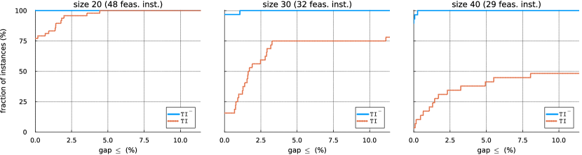
Figure 2: Optimality gaps of TI^- and TI on the subset of instances feasible without task-splitting.

Impact of heuristics

Motivated by the preceding results, we proceed with the analysis of the impact of the heuristics introduced in Section 4.2. To this end, Figure 3 shows the cumulative percentages of instances for which the optimality gap is below a certain threshold when simply solving the time-indexed formulation (TI) is solved in isolation or when it is solved in conjunction with the time-indexed or the MTZ-based heuristic (TI+HTI and TI+HMTZ). In these experiments, all 159 instances that are feasible for the HHCRSP-TS are considered. Figure 3 shows that both variants of the heuristic result in significant performance improvements, especially for instances of size 30 and 40. For small instances of size 20, we observe that they can be solved relatively well without the use of heuristics. Consequently, the observed differences between the three variants are minimal for these instances. Both versions with heuristics identify a feasible solution for one additional instance, and the optimality gaps are nearly identical. However, a clear performance gain is observed for the instances of size 30, for which TI could not find any feasible solution in 12 cases. Here, TI+HTI finds feasible solutions for 9 additional instances, while feasible solutions to all instances are found by the MTZ variant TI+HMTZ. The performance gain becomes even larger for the instances of size 40. In these instances, TI, TI+HTI, and TI+HMTZ find feasible solutions for 20, 32, and 39 out of the 40 instances, respectively. In addition to finding more feasible solutions, we also observe that including the heuristics significantly reduces the final optimality gaps in instances of size 30 and size 40. We observe that variant TI+HMTZ with the MTZ-based primal heuristic outperforms the time-indexed variant TI+HTI with respect to the number of instances for which solutions are found and when considering the final optimality gaps.

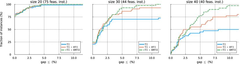
Figure 3: Optimality gaps of TI, TI+HTI, and TI+HMTZ.

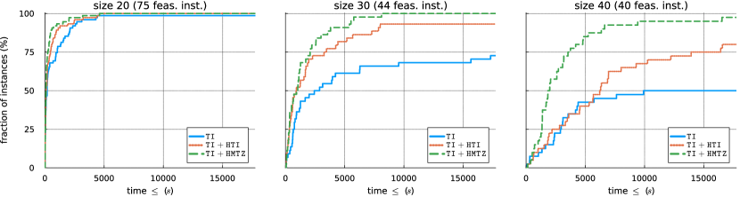
Figure 4: Runtimes [s] until the first solution for TI, TI+HTI, and TI+HMTZ.

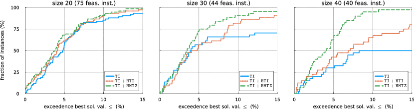
Figure 5: Relative gaps between the first solution found by TI, TI+HTI, and TI+HMTZ and overall best known solution. The results are cutoff at 15%.

Further insights about the positive contributions of the proposed heuristics for the solution process are gained by Figures 4 and 5 in B.1. These figures show the relative amounts of instances for which the first solution is found within a given time (Figure 4) and for which the relative difference between the objective value of this first solution and the overall best-known solution for that instance is below a certain threshold (Figure 5).

These results show that the heuristic procedures typically find solutions earlier during the solution process and that the initial solutions they find are of superior quality to the initial solutions of variant TI obtained by Gurobi’s general-purpose heuristics. Both of these positive effects are more pronounced for TI+HMTZ than for TI+HTI and also increase with an increasing instance size. An in-depth analysis of the results showed that the first feasible solution is found by a primal heuristic in 47.5% and 87.5% of all instances of size 40 in the case of TI+HTI and TI+HMTZ, respectively. Variant TI+HTI with the time-indexed primal heuristic required an average of 455 attempts, each taking 0.7 seconds, until a feasible solution was found from a fractional solution. In contrast, variant TI+HMTZ based on the MTZ formulation only required 61 calls lasting on average 0.4 seconds. Given the clear benefits of TI+HMTZ over the other two alternatives, we will concentrate on this variant in the following paragraph.

With regard to the quality of initial solutions, we observe that 75% and 67.5% of those found by TI+HMTZ are, at most, 5% worse than the best-known final solutions (among the TI, TI+HTI, and TI+HMTZ methods) for instances of size 30 and 40, respectively. The improvement step contributes significantly to their quality. Focusing on the instances of size 40, an initial solution found by the MTZ-based primal heuristic could be enhanced by the improvement heuristic in 94.3% of the cases, reducing the objective value by 6.0% on average. The time required to apply the improvement heuristic on instances with size 40 is usually below 30 seconds (on average 94 seconds due to one outlier reaching the time limit). We note that for instances of size 40, the improvement heuristic also consistently enhanced initial solutions found by Gurobi’s general-purpose heuristics, in which case its average objective value reduction was equal to 0.9%. Furthermore, on all instances of size 40, it enhanced 56.9% of the solutions found by Gurobi after the initial one. The average relative cost decrease was 0.2% and the corresponding average runtime 0.3 seconds.

Overall, variant TI+HMTZ outperforms the variants TI+HTI and TI, and the obtained results demonstrate the performance of the proposed heuristic procedure. Consequently, we will also use variant TI+HMTZ to obtain results for the HHCRSP-TS-TT.

6.2 Impact of task-splitting

The impact of introducing task-splitting for HHC providers is discussed in three parts. First, we explore the effect on staff requirements. Second, we discuss the consequences for the daily work schedules of caregivers. Third, we describe the change in operational costs achieved through the utilization of task-splitting options. Since (proven) optimal solutions are not available for most task-splitting instances, the analyses compare the best available solution without task-splitting to the best available solution when task-splitting is permitted.

Required staff and staff composition

One primary motivation for considering task-splitting is that it may enable a better use of the available staff. To ascertain under which conditions such an effect can be observed, we present in Table 4 the number of instances for which a feasible schedule for caregivers exists with and without task-splitting. We first observe that the additional planning flexibility resulting from task-splitting significantly increases the number of cases for which all patient visits can be performed with the available caregivers. For instances of size 20, task-splitting increases the number of feasible instances from 48 to 75, representing a +56% increase. For instances of size 30, the increase is from 32 to 44 (+38%) and for instances of size 40, the increase is from 29 to 40 (+38%).

The results also indicate that task-splitting allows for the performance of patient visits with a less medically trained staff compared to a situation without task-splitting possibilities. This can be observed from the results for scenarios with balanced patient requirements in combination with a practically or moderately trained staff, where most infeasible instances become feasible thanks to task-splitting. In contrast, most instances remain infeasible for a practically or moderately trained staff in scenarios with medical patient visit requirements. In addition to the extra planning options offered by the ability to split parts between different caregivers at different moments in time, other advantages of task-splitting are also utilized. The amount of tasks within a certain time frame that require more medically trained caregivers can be reduced by performing one split part of a splittable visit by a more practically trained caregiver, if allowed. In instances that become feasible through task-splitting, this advantage is utilized in approximately 73% of the split visits. Task-splitting can reduce the number of tasks that must be performed within a certain timeframe since some split visits have an extended, relaxed starting time window (see Section 5). However, this factor seems to play a less prominent role than the qualification relaxation and is exploited in $\pm$35% of the splits in instances that became feasible through task-splitting.

We conclude that task-splitting can help increase planning options and reduce the number of tasks that require a specifically trained caregiver type. Task-splitting may, therefore, help to counteract issues arising from staff shortages, especially for medically trained caregivers.

Table 4: Number of feasible instances with and without task-splitting.

			number of feasible instances
			prac. train. staff		moder. train. staff		medic. train. staff		only medic. staff
size	#	visit req.	no split.	split.	no split.	split.	no split.	split.	no split.	split.
20	10	general	4	10	5	10	10	10
		balanced	1	5	3	10	8	10	10	10
		medical	0	0	0	0	7	10
30	5	general	5	5	5	5	5	5
		balanced	0	5	3	5	5	5	5	5
		medical	0	1	0	3	4	5
40	5	general	5	5	5	5	5	5
		balanced	0	5	0	5	5	5	5	5
		medical	0	0	0	0	4	5

Staff schedules

To explore the impact of task-splitting on the daily work schedule of caregivers, Table 5 lists the percentages of the total working time that caregivers spend on performing care. We observe that concerns may arise regarding the impact of task-splitting on caregiver work satisfaction. They include increased travel and/or waiting time or overly dense plannings. However, for the instances considered, we observe that on average, prior to splitting, 84.7% of the total working time of the caregivers consisted of patient visits, while after splitting, this decreased slightly to 84.0%. Therefore, it can be concluded that task-splitting does not seem to significantly change the percentage of working time caregivers spend providing care. This could be of interest to HHC providers when counteracting potential staff concerns. Furthermore, Table 5 does not demonstrate any clear relationships between the change in patient time and the considered scenario (e.g., see general support visit requirements in combination with different staff compositions or a medically trained staff composition with different visit requirements for size 30 instances). The results indicate that a higher percentage of time is spent on patient care in scenarios where more medically trained caregivers become available (compare combination of general support visit requirements with a practically or only medically trained staff) or where visits require less medical tasks (moving from medical visit requirements to general support requirement for a medically trained staff). The underlying reason may be that inefficient routing decisions and waiting times can be avoided if a smaller proportion of the caregivers can only perform a subset of the patient visits.

Our findings indicate that task-splitting has no significant impact on the total working time of the caregivers. The total working time is, on average, reduced by only 0.8% across the instances considered. Indeed, the relative increase in travel time due to task-splitting (+9%) is compensated by a reduction in patient visiting and waiting time.

Although the impact of task-splitting on the total working time is limited, it does impact the division of work among caregivers. In the set of test instances, the average percentage of total working time assigned to level 3 caregivers decreased by 4.3 percentage points, indicating a reduction in their participation in tasks requiring a level 1 or level 2 caregiver. The consequence of level 3 caregivers performing fewer care tasks is that mainly level 1 caregivers work longer. Therefore, one of the potential benefits of task-splitting may be that caregivers spend relatively more time on tasks aligned with their education. An overview of the division of working time among the three qualification levels with and without splitting is presented in B.2.

Table 5: Percentage of the total working time spent on patient care. Only instances that are feasible without task-splitting are considered.

			percentage of working time spent on patient care
			prac. train. staff		moder. train. staff		medic. train. staff		only medic. staff
size	$\#$	visit req.	no split.	split.	no split.	split.	no split.	split.	no split.	split.
20	10	general	78.0	77.2	80.8	80.5	82.6	82.5
		balanced	80.3	82.0	77.2	79.0	80.4	80.8	86.2	85.8
		medical					79.3	78.5
30	5	general	85.2	83.9	87.0	85.8	87.5	86.5
		balanced			84.2	83.1	86.1	85.2	89.8	89.1
		medical					85.1	83.2
40	5	general	86.2	84.0	87.8	86.4	88.5	87.9
		balanced					87.3	86.1	91.3	90.4
		medical					85.6	84.0

Operational costs

The possibility of task-splitting not only reduces the staffing requirements for the instances studied, but also allows for schedules with lower operational costs. This is illustrated in Table 6, which summarizes the decrease in objective value due to task-splitting for the minimization of both operational costs and travel time. The smallest gains occur in the instances where each caregiver can perform all patient visits. In the scenario with only medically trained staff, the flexibility gained through task-splitting reduces the total costs by more than 1.1%. This decrease is primarily achieved through splits that reduce the combined patient time. The gains from task-splitting increase for scenarios that differentiate between the qualifications of the caregivers. This effect is particularly strong in scenarios where a large proportion of the caregivers are unable to perform a subset of the visits. Focusing, for instance, on the general support scenario, we observe that the gain due to task-splitting increases each time the staff composition shifts more to a practically trained staff, eventually reaching a decrease in operational costs of more than 7%. Without task-splitting, medically trained caregivers must perform all visits that include a highly medical task. However, due to splitting, all types of caregivers (i.e., 1, 2 and 3) can perform split parts that only require a practically trained caregiver. The lower wages for level 1 and level 2 caregivers can make it beneficial for more practically trained caregivers to perform these split parts. Consequently, if the staff composition changes more in this direction, then the care load of split parts can be assigned to the more readily available cheaper caregivers, resulting in a higher benefit in terms of operational costs. Additionally, assigning tasks to level 1 or level 2 caregivers becomes more attractive when relatively more of them become available, as simultaneously fewer caregivers of other types become available so their corresponding routing options decrease.

Table 6: Objective value decrease due to task-splitting when minimizing operational costs (o.c.) or travel time (t.t.).

			decrease in objective value due to task-splitting (%)
			prac. train. staff		moder. train. staff		medic. train. staff		only medic. staff
size	$\#$	visit req.	o.c.	t.t.	o.c.	t.t.	o.c.	t.t.	o.c.	t.t.
20	10	general	3.83	4.80	2.39	0.45	4.33	3.39
		balanced	4.68	0.39	4.26	1.93	5.97	1.45	1.16	1.50
		medical					8.08	9.08
30	5	general	7.26	6.72	3.37	2.60	2.23	1.40
		balanced			4.66	9.88	2.72	2.22	1.09	0.64
		medical					3.73	6.44
40	5	general	6.89	6.22	3.95	7.54	2.83	1.77
		balanced					6.00	2.19	1.46	1.17
		medical					4.58	8.55

The main conclusions drawn from the results discussed in this section are that task-splitting can reduce the operational costs for an HHC provider, help to deal with staff shortages (in particular of highly qualified caregivers), and help to ensure a better match between qualifications of caregivers and the tasks assigned to them. Our results also showed that these benefits do not come at the price of overly dense schedules for caregivers, which could be detrimental to their work satisfaction.

6.3 Impact of objective

In this section, we will address the third main goal of our computational study, which is to assess to what extent the observed benefits of task-splitting depend on the specific choice of the objective function. To this end, we compare the results for operational cost minimization (HHCRSP-TS) with those for travel time minimization (HHCRSP-TS-TT). We will first focus on reducing objective function values, then analyze the effect of task-splitting on staff schedules, and lastly compare the percentage of split options utilized in the solutions.

Objective function value

Table 6 presents the reduction in objective function values thanks to task-splitting for operational cost minimization (discussed in Section 6.2) and travel time minimization. The objective of the HHCRSP-TS-TT does not consider wage differences between the different caregiver types. Moreover, additional travel time due to task-splitting cannot be compensated with reduced care or shorter waiting times. Table 6 illustrates that task-splitting can be interesting for HHC providers when minimizing travel time. Splitting visits, for example, can create additional routes that contribute to a solution with a lower total travel time. Although the average reduction of the objective function value is slightly smaller compared to operational cost minimization (3.7% vs 4.0%), we consistently observe gains in all considered scenarios that are sometimes even larger than those for the HHCRSP-TS. The results clearly indicate that task-splitting is not only relevant when minimizing the operational costs and considering wage differences between different types of caregivers. It is also relevant when minimizing travel time.

Staff schedules

To further explore the differences in solutions obtained for the two objectives, Table 7 reports the percentage of time caregivers spend on patient care. To facilitate a fair comparison, the starting times of patient visits for solutions found in variant HHCRSP-TS-TT are improved during post-processing to avoid unnecessary waiting time in the schedules. We note that no feasible solution could be found for a single instance of size 40 when minimizing travel time. Consequently, this instance is excluded from this comparison. The largest difference in the percentage of working time spent on patient care occurs if only medically trained staff is available. In these scenarios, minimizing travel time instead of operational costs results in caregiver schedules for which the percentage of working time spent on patient care is, on average, 8.5 percentage points lower. A summary of all considered benchmark instances indicates that the percentage of a workday that caregivers spend on providing care is, on average, four percentage points higher when minimizing operational costs. Since waiting time is not considered in the objective of the HHCRSP-TS-TT, the length of the resulting schedules is not optimized. As a result, caregivers spend, on average, approximately 5.6% of their workday waiting. In contrast, the schedules obtained with HHCRSP-TS, which minimizes operational costs, are much more compact and efficient for caregivers, requiring less working time for the same amount of care. In addition to potentially shorter workdays, which are interest for caregivers, the operational costs objective is also relevant for HHC providers. It can create time for additional care tasks and may also reduce (variable) labor costs. Therefore, an operational cost objective seems to be a more natural option for both stakeholders.

We note that the division of working time among the different caregiver types is different for both objective functions. When minimizing travel time instead of operational costs, a larger portion of the total working time is assigned to medically trained caregivers in a situation without task-splitting. After task-splitting, the division of working time between the different caregiver types only remains roughly the same for travel time minimization.

Table 7: Percentage of the total working time spent on patient care when minimizing the operational costs (o.c.) or travel time (t.t.). Only those instances for which a feasible solution is found in both cases are considered. The care initiation times for the schedules corresponding to travel time minimization are improved such that they minimize the total working time.

			percentage of working time spent on patient care
			prac. train. staff		moder. train. staff		medic. train. staff		only medic. staff
size	$\#$	visit req.	o.c.	t.t.	o.c.	t.t.	o.c.	t.t.	o.c.	t.t.
20	10	general	79.4	76.3	81.9	77.2	82.5	76.4
		balanced	79.0	75.8	80.3	76.6	81.8	76.8	85.8	76.4
		medical					80.1	76.4
30	5	general	83.9	83.5	85.8	82.9	86.5	82.4
		balanced	81.5	82.4	83.6	80.3	85.2	82.4	89.1	83.6
		medical	76.6	72.8	80.8	76.2	83.8	82.6
40	5	general	84.0	81.8	86.4	82.0	87.9	83.1
		balanced	84.2	83.2	83.7	81.5	86.1	82.8	90.4	80.8
		medical					84.2	82.9

Percentage of split options utilized

Table 8 shows the percentages of utilized splits for the two considered problem variants. The results indicate that an increase in the skill levels of the available staff (from practically trained staff to only medically trained staff) results in a decrease in the number of used splits because higher-skilled staff are capable of performing more tasks. Moreover, we observe a tendency for additional task-splitting when visits require more medical tasks (i.e., moving from general visit requirements to medical requirements) for a given staff composition (practically trained staff up to medically trained staff). A comparison of the results for the two objective functions reveals that a greater number of splits occur for the operational cost minimization objective. This may be attributed to the fact that, in the case of operational cost minimization, extra travel time can be compensated by a reduction in patient time and/or waiting time, thereby making task-splitting more beneficial. Wage differentiation also stimulates task-splitting, resulting in the execution of tasks by the cheapest, appropriately qualified caregiver. In turn, the comparably low number of splits for the travel time minimization objective suggests that even a few splits (see Table 8) can have benefits for caregiver planning in terms of the number of instances that are feasible and the reduction in terms of objective value that can be achieved (see Table 4 and Table 6).

Table 8: Percentage of utilized splits when minimizing operational costs (o.c.) or travel time (t.t.). Only instances that result in a feasible solution in both cases are considered.

			percentage of utilized splits
			prac. train. staff		moder. train. staff		medic. train. staff		only medic. staff
size	$\#$	visit req.	o.c.	t.t.	o.c.	t.t.	o.c.	t.t.	o.c.	t.t.
20	10	general	40	21	29	16	29	8
		balanced	43	27	35	19	32	6	21	3
		medical					47	18
30	5	general	44	13	32	6	28	6
		balanced	52	33	45	17	39	5	19	7
		medical	60	47	59	37	58	11
40	5	general	46	9	38	11	32	4
		balanced	60	35	52	22	48	3	26	5
		medical					45	15

7 Conclusions

This is the first paper to formally examine the potential of incorporating task-splitting possibilities into home healthcare (HHC) planning. Home healthcare routing and scheduling problems are widely studied due to the relevance of affordable and reliable HHC. Consequently, numerous problem variants have been proposed in the literature (e.g., Oladzad-Abbasabady et al. (2023); Erdem et al. (2022)). Existing research focuses on the construction of efficient caregiver schedules, while typically accounting for varying qualifications and preferences among caregivers, specific service and time requests for patient visits, and occasionally temporal restrictions between multiple visits to the same patient. However, none of the papers studying home healthcare planning explores the potential of splitting patient visits consisting of multiple tasks into separate visits.

This paper presents a novel problem variant of the Home Healthcare Routing and Scheduling Problem (HHCRSP), in which the decision to split patient visits is integrated into the planning process. The objective is to design caregiver routes and schedules that minimize operational costs for home healthcare providers. The proposed model formulation allows split parts to have potentially wider visiting times, a shorter or longer combined duration, and to use lower-qualified caregivers than the unsplit visit. Temporal dependencies can be imposed between all types of patient visits. Two novel integer linear programming formulations are presented (a MTZ formulation and a time-indexed variant) and an effective branch-and-bound solution framework is developed. The solution framework performance on the time-indexed variant is enhanced with pre-processing techniques and one of the two proposed heuristics, which is embedded as a primal and improvement heuristic in the branch-and-bound solution approach.

An extensive computational analysis examines the managerial and computational impacts of task-splitting. In the instances considered, task-splitting enables care to be provided with less caregivers or caregivers with less medical training and reduces operational costs for HHC providers. This enables a more optimal use of the available staff. Task-splitting can also help to ensure that caregivers spend relatively more time on care tasks commensurate with their qualification level. Another observation is that task-splitting also has benefits in settings when the objective is to minimize the total travel time. From a computational point of view, the results demonstrate that introducing task-splitting poses a significant additional computational challenge due to the increase in routing options and synchronization requirements. A general-purpose solver was not able to find solutions for feasible instances within the time limit. The primal heuristic based on the MTZ formulation is capable of partially overcoming this issue; it found solutions for almost all of the considered test instances.

Our research demonstrates the potential of the proposed formulations and solution framework and indicates the benefits of task-splitting. However, these findings could be strengthened by conducting an extensive pilot project in close collaboration with HHC providers. Such research could provide additional insights into the savings (in cost or working time) that can be achieved in practice, along with the conditions under which task-splitting can be embraced by staff and patients alike. In addition, one might discover the need to incorporate additional features into the model formulation, such as considering a multi-period scheduling horizon, patient preferences on limiting the number of different caregivers, caregivers asking for workload balancing schedules, etc. A second, related avenue for further research is the development of solution methods capable of solving larger problem instances within a limited computation time. Although the methodology proposed in the current paper is capable of handling a wide variety of temporal restrictions associated with task-splitting, its computational performance for the test instances consisting of 40 visits is too high to dynamically support the daily planning of larger (home healthcare) service providers. Consequently, we see a potential for the development of alternative exact or heuristic solution frameworks to address synchronization constraints in a multitude of industries and problem settings. Since real-life travel and service times can be non-deterministic, and demand can be dynamic, there is also the potential for the development of other dedicated solution approaches.

Appendix A Detailed description benchmark instances

To explore the impact of task-splitting on home healthcare planning, we generated a set of benchmark instances based on those introduced by Bredström and Rönnqvist (2008). These instances were designed to mimic a simpler HHCRSP compared to the HHCRSP-TS, which does not include qualification requirements for patient visits and only allows for strict synchronization restrictions. They have also been utilized in computational experiments of other papers studying HHCRSPs with synchronization (see, e.g., Masmoudi et al. (2023); Euchi et al. (2020); Decerle et al. (2019)). We adapted the instances of Bredström and Rönnqvist (2008) with a small visiting time window (five distinct time window widths are available). Each of these instances considers a planning horizon of 9 hours, has one caregiver per five patient visits, and requires strict synchronization between one pair of visits out of every ten patient visits.

In order to generate instances for the HHCRSP-TS based on the Bredström and Rönnqvist (2008) instances, we introduced qualification requirements for visits, qualifications of caregivers, and task-splitting possibilities. When introducing each of these elements, our aim was to select reasonable parameter values such that the instances mimic situations that can occur in real life. For each original Bredström and Rönnqvist (2008) instance, we created different scenarios that vary the qualification requirements of visits and the composition (qualification) of the available staff. These scenarios were used in Section 6 to gain insights into the potential benefits of task-splitting. We use three ordered qualification levels (1, 2, and 3) that reflect current practice in the Netherlands, where caregivers are typically categorized based on their ability to provide general support, perform medical interventions, or administer medication. Caregivers can perform tasks whose qualification requirement does not exceed their qualification level. Following Yin et al. (2023) and Qiu et al. (2022), we assign a cost to each qualification level proportional to its number, i.e., $e^{1}=1$, $e^{2}=2$, and $e^{3}=3$.

Qualification requirements

We vary the proportion of visits requiring specific qualification levels by using the following three qualification requirement profiles:

• General support requirements (50% level 1, 25% level 2, 25% level 3)

• Balanced requirements (33.3% level 1, 33.3% level 2, 33.3% level 3)

• Medical requirements (25% level 1, 25% level 2, 50% level 3)

For each of these scenarios, the qualification requirement for each visit is randomly selected according to these probabilities. When distributing a specific number of visits, the required number of tasks with a specific qualification level can be non-integer due to the utilized percentage. We first round non-integer values down. Any remaining visits are then allocated sequentially to qualification levels 2, 1, and 3. To ensure a fair comparison between different scenarios, we maintain the required qualification level for as many visits as possible when transitioning between scenarios. For example, the set of level 1 tasks in the balanced scenario is a subset of those in the general support scenario.

Qualifications of caregivers

We consider four scenarios for the qualification levels of caregivers:

• Practically trained (50% level 1, 25% level 2, 25% level 3)

• Moderately trained (25% level 1, 50% level 2, 25% level 3)

• Medically trained (25% level 1, 25% level 2, 50% level 3)

• Only medically trained (0% level 1, 0% level 2, 100% level 3)

When allocating a specific number of staff members, we round non-integer values of staff members with a specific qualification down. Any remaining staff members are successively assigned to qualification level 3, 2, and 1. Notably, if all caregivers have qualification level 3, then the required qualification level of the visits becomes irrelevant as all caregivers can perform all tasks.

We derive ten benchmark instances for each initial instance by Bredström and Rönnqvist (2008). These instances are the result of combining the three different visit qualification profiles with the first three staff compositions plus the one in which qualification levels become irrelevant (100% level 3 staff). This approach enables us to analyze various scenarios in our computational study, which aims to gain insights into the potential of task-splitting under different, practically relevant circumstances. For example, by combining balanced or medical qualification requirements with a practically trained staff, we mimic a situation in which there is a shortage of medically trained caregivers.

To analyze performance differences between the different solution procedures, we also consider instances of different sizes. Bredström and Rönnqvist (2008) consider 5 instances of 20 visits, 3 instances of 50 visits, and 2 instances of 80 visits. Since solving instances of size 50 and size 80 requires substantial computational resources, we scale those instances down by selecting a random subset of visits. From each of those instances, we generate new instances for the HHCRSP-TS of sizes 20, 30 and 40 while maintaining the ratio of synchronization visits. Together with the 5 original instances of size 20, this results in 10 instances of size 20, 5 instances of size 30, and 5 instances of size 40 for the HHCRSP-TS. For instances generated from the larger original ones of size 50 and size 80, we ensure that the instances of size 30 extend those of size 20, and instances of size 40 extend those of size 30. In other words, we ensure that the visits of a smaller instance are also included in a larger one with the same characteristics. Since we combine each of them with the 10 scenarios, we also maintain the required qualification levels of the visits within a certain scenario, regardless of the size of the instance. This helps to compare how the instance size affects the computational need of the methods and how the instance size affects the impact of task-splitting.

Moreover, the variation in visit requirements and staff composition, together with the variation in instance size, results in a variety of instances to challenge the proposed solution approaches. It also allows us to gain insights into the potential impact of task-splitting on a highly diverse test set.

Task-splitting

To complete the benchmark instances after introducing all the aforementioned aspects, we add the possibility to split tasks. To this end, all visits with a duration of at least one hour are considered as splittable. Shorter visits are not identified as splittable, as they are likely associated with a single task or short activities. For each splittable visit $v\in S$, we create two split components $v_{1}$ and $v_{2}$ at the same location. The following paragraphs describe how different parameters of the two split components (durations, qualification levels, time windows, temporal dependencies) are made. To facilitate an analysis of various effects, we ensure that these (randomized) decisions are made identical in all final instances that correspond to the same original instance by Bredström and Rönnqvist (2008). Insights into the number of splittable visits within the instances considered are provided in Table 2.

To set the duration of individual split components, we first decide on their combined duration. Here, we consider cases in which the combined duration of the split components is equivalent to the duration of the original visit and those in which a split can reduce (e.g., due to removal of waiting time) or increase (e.g., due to double start-up time) the total duration. Since we assume that these effects are more pronounced for longer visits, we set the combined duration of the two split parts equal to the duration of the original visit for all visits whose duration is below 75 minutes. For longer visits, the combined duration of the split components is either decreased by 15 minutes, remains the same, or is increased by 15 minutes, each with a probability of $\frac{1}{3}$. Subsequently, the duration of each individual split component is determined by randomly splitting the combined duration into two while ensuring a minimum duration of at least 30 minutes per split part.

The required qualification level of the split components will usually be equal to the one of the original visit. However, there are cases where the qualification requirements for one of the split components can be relaxed (e.g., when splitting bathing and medical care into two separate visits). To account for this, we randomly select one of the split components whose required qualification level is set to level 1 (i.e., it can be performed by all caregivers) with a probability of 0.75.

The time windows of the split components are based on the earliest starting time and latest completion time of the original visit. A splittable visit $v\in S$ with time window $[\alpha_{v},\beta_{v}]$ can start no later than time $\beta_{v}$, so it must be completed before $\beta_{v}+d_{v}$. Assuming that this completion time holds for all tasks within the visit, we derive the permitted starting time window $[\alpha_{v},\beta_{v}+d_{v}-d_{v_{p}}]$ for each split component $p\in\{1,2\}$. Additionally, we incorporate the possibility that one of the split components may have less restricted time requirements than the original visit (e.g., when splitting domestic help and medical care). Therefore, we randomly select one split component and increase its latest starting time by one hour with a probability of 0.75.

We randomly impose one of the following three temporal dependencies between the split components: no temporal dependency, precedence, and disjunction. No temporal dependency occurs when a parallel execution of the two split tasks is possible (e.g., medical and domestic help). A precedence temporal dependency arises if one of them must be finished before the other (e.g., bathing before wound care). In the latter case, a split component for which the latest starting time has been extended (see above) must be performed second, while the order is randomly determined otherwise. A disjunctive requirement occurs when both split components require contact with the patient but do not have a specific order (e.g., bathing and some medical care). For disjunctive and precedence temporal dependencies, we ensure that any potential waiting time removed from a caregiver visit due to a split is still present for the patient, i.e., when the combined duration of the split parts is lower than that of the original visit.

Finally, two splittable visits may require strict synchronization and thus have identical time windows and durations. In this case, they are split in the same way (relaxed caregiver qualifications are generated independently), and the split parts must be performed together. Consequently, only precedence or disjunction restrictions are enforced between the split parts, as having no temporal dependency could result in four caregivers performing care at a patient’s home simultaneously.

Appendix B Additional results

B.1 Performance heuristics

B.2 Division of working time over the different caregiver types

Tables 9, 10, and 11 provide an overview of the allocation of total working time among the three different types of caregivers for the instances considered, with and without task-splitting. In every scenario except for one, the percentage of working time assigned to level 3 caregivers decreases because of the introduction of task-splitting. Conversely, we observe that the percentage of total working time assigned to level 1 caregiver increases in each scenario.

Table 9: Percentage of the total working time assigned to level 1 caregivers. Only instances feasible without task-splitting are considered.

			percentage of working time assigned to level 1 caregivers
			prac. train. staff		moder. train. staff		medic. train. staff		only medic. staff
size	$\#$	visit req.	no split.	split.	no split.	split.	no split.	split.	no split.	split.
20	10	general	46.6	53.3	34.5	37.4	32.6	34.5
		balanced	41.0	42.5	33.3	35.7	29.5	33.2	0.0	0.0
		medical					19.5	32.0
30	5	general	50.2	57.1	22.3	24.2	23.5	24.2
		balanced			21.1	23.4	20.8	22.8	0.0	0.0
		medical					19.7	22.6
40	5	general	50.0	57.9	33.3	35.2	33.5	35.1
		balanced					28.8	33.6	0.0	0.0
		medical					25.6	31.0

Table 10: Percentage of the total working time assigned to level 2 caregivers. Only instances feasible without task-splitting are considered.

			percentage of working time assigned to level 2 caregivers
			prac. train. staff		moder. train. staff		medic. train. staff		only medic. staff
size	$\#$	visit req.	no split.	split.	no split.	split.	no split.	split.	no split.	split.
20	10	general	24.9	18.8	36.4	33.7	27.9	30.2
		balanced	32.0	29.2	32.6	30.3	29.4	30.3	0.0	0.0
		medical					26.2	20.2
30	5	general	20.7	19.9	50.4	52.6	39.7	42.2
		balanced			44.5	48.4	39.1	40.1	0.0	0.0
		medical					31.2	35.6
40	5	general	22.8	20.0	39.6	42.6	31.9	33.3
		balanced					30.2	31.7	0.0	0.0
		medical					23.7	24.9

Table 11: Percentage of the total working time assigned to level 3 caregivers. Only instances feasible without task-splitting are considered.

			percentage of working time assigned to level 3 caregivers
			prac. train. staff		moder. train. staff		medic. train. staff		only medic. staff
size	$\#$	visit req.	no split.	split.	no split.	split.	no split.	split.	no split.	split.
20	10	general	28.4	28.0	29.1	28.8	39.5	35.3
		balanced	27.0	28.3	34.1	34.0	41.1	36.5	100.0	100.0
		medical					54.4	47.8
30	5	general	29.1	23.0	27.3	23.2	36.8	33.6
		balanced			34.4	28.2	40.1	37.1	100.0	100.0
		medical					49.1	41.8
40	5	general	27.1	22.0	27.0	22.2	34.6	31.7
		balanced					41.0	34.8	100.0	100.0
		medical					50.7	44.1

Appendix C Adjustments to temporal dependencies due to pre-processing

The pre-processing step of Section 4.1, replacing constraints (2f) and (2g) with (3), requires the addition of extra temporal dependencies if at least one visit has multiple temporal dependencies with other visits. Consider a visit $v\in V$ that has a temporal restriction with visit $u\in V$ and visit $w\in V$, i.e. $\{u,v\}\in D$ and $\{v,w\}\in D$. Let $t^{*}_{v}$ be the arrival time and $t^{\prime}_{v}$ be the departure time at visit $v$, where we require $t^{*}_{v}\neq t^{\prime}_{v}$. Before the pre-processing step of removing redundant travel arcs, time $t^{\prime}_{v}$ had to satisfy the temporal restrictions with $u$ and $w$. Now each time within interval $[t^{*}_{v},t^{\prime}_{v}]$ can be used. As a result, a solution where temporal dependency $\{u,v\}$ requires $t^{*}_{v}$ while temporal dependency $\{v,w\}$ requires time $t^{\prime}_{v}$ is feasible. Since $v$ cannot start at two different moments in time, such solutions must be excluded. Specifically, we have to ensure that there is at least one time point within $[t^{*}_{v},t^{\prime}_{v}]$ that satisfies the temporal dependence with $u$ and with $w$. This is done by introducing temporal dependencies between $u$ and $w$, specifically those that were previously implicitly ensured.

Before specifying the temporal restrictions between $u$ and $w$, we first recap the explicit temporal restriction between the starting times of $u$ and $v$ and $v$ and $w$. We denote the starting time of visit $u$, $v$, and $w$ with $t_{u}$, $t_{v}$, and $t_{w}$, respectively. Depending on the value of precedence variable $p_{uv}$, the following restrictions arise from temporal dependency $\{u,v\}$:

if $$p_{uv}=1 t_{v}\in[t_{u}+\delta^{\mathrm{min}}_{uv},t_{u}+\delta^{\mathrm{max}}_{uv}]$$: (4)

$$\Leftrightarrow\ t_{u}\in[t_{v}-\delta^{\mathrm{max}}_{uv},t_{v}-\delta^{\mathrm{min}}_{uv}]$$ (5)

if $$p_{uv}=0 t_{u}\in[t_{v}+\delta^{\mathrm{min}}_{vu},t_{v}+\delta^{\mathrm{max}}_{vu}]$$: (6)

$$\Leftrightarrow\ t_{v}\in[t_{u}-\delta^{\mathrm{max}}_{vu},t_{u}-\delta^{\mathrm{min}}_{vu}]\quad$$ (7)

Similarly, depending on the value of $p_{vw}$, temporal dependency $\{v,w\}$ induces constraints

if $$p_{vw}=1 t_{w}\in[t_{v}+\delta^{\mathrm{min}}_{vw},t_{v}+\delta^{\mathrm{max}}_{vw}]$$: (8)

$$\Leftrightarrow\ t_{v}\in[t_{w}-\delta^{\mathrm{max}}_{vw},t_{w}-\delta^{\mathrm{min}}_{vw}]$$ (9)

if $$p_{uv}=0 t_{v}\in[t_{w}+\delta^{\mathrm{min}}_{wv},t_{w}+\delta^{\mathrm{max}}_{wv}]$$: (10)

$$\Leftrightarrow\ t_{w}\in[t_{v}-\delta^{\mathrm{max}}_{wv},t_{v}-\delta^{\mathrm{min}}_{wv}]$$ (11)

These temporal restrictions between $u$ and $v$ and $v$ and $w$ naturally induce temporal restrictions between $u$ and $w$, since $t_{u}$ and $t_{w}$ are linked with each other through $t_{v}$. Specifically, for each combination of a value of $p_{uv}$ and $p_{vw}$, the bounds on the starting times of $v$ with respect to $u$ and $w$ can be combined to derive the permitted difference between starting times $t_{u}$ and $t_{w}$ of visits $u$ and $w$, respectively. The various combinations of $p_{uv}$ and $p_{vw}$ result in the following restrictions:

• Case $p_{uv}=1$ and $p_{vw}=1$: by using bounds (4) on the starting time of $v$ with respect to $u$ in (8), we observe the minimum and maximum difference of the starting time $t_{w}$ with respect to $t_{u}$. Specifically, $t_{w}\geq t_{w}$ is required with $t_{w}\in[t_{u}+\delta^{\mathrm{min}}_{uv}+\delta^{\mathrm{min}}_{vw},t_{u}+\delta^{\mathrm{max}}_{uv}+\delta^{\mathrm{max}}_{vw}]$.

• Case $p_{uv}=1$ and $p_{vw}=0$: by using bounds (4) on the starting time of $v$ with respect to $u$, but this time in (11), we observe the temporal relation $t_{w}\in[t_{u}+\delta^{\mathrm{min}}_{uv}-\delta^{\mathrm{max}}_{wv},t_{u}+\delta^{\mathrm{max}}_{uv}-\delta^{\mathrm{min}}_{wv}]$. Then, splitting the results for the two starting orders of $u$ and $w$ gives:

  • $t_{w}\in[t_{u}+\max\{\delta^{\mathrm{min}}_{uv}-\delta^{\mathrm{max}}_{wv},0\},t_{u}+\delta^{\mathrm{max}}_{uv}-\delta^{\mathrm{min}}_{wv}]$ for $t_{w}\geq t_{u}$, whose starting order is only possible when $\delta^{\mathrm{max}}_{uv}-\delta^{\mathrm{min}}_{wv}\geq 0$.

  • $t_{u}\in[t_{w}+\max\{\delta^{\mathrm{min}}_{wv}-\delta^{\mathrm{max}}_{uv},0\},t_{w}+\delta^{\mathrm{max}}_{wv}-\delta^{\mathrm{min}}_{uv}]$, whose starting order requires $\delta^{\mathrm{max}}_{wv}-\delta^{\mathrm{min}}_{uv}$.

• Case $p_{uv}=0$ and $p_{vw}=1$: using bounds (7) on the starting time of visit $v$ with respect to $u$ in (8), we observe that $t_{w}\in[t_{u}-\delta^{\mathrm{max}}_{vu}+\delta^{\mathrm{min}}_{vw},t_{u}-\delta^{\mathrm{min}}_{vu}+\delta^{\mathrm{max}}_{vw}]$. Splitting the results for the two starting orders of visits $u$ and $w$ once again, we arrive at:

  • $t_{w}\in[t_{u}+\max\{-\delta^{\mathrm{max}}_{vu}+\delta^{\mathrm{min}}_{vw},0\},t_{u}-\delta^{\mathrm{min}}_{vu}+\delta^{\mathrm{max}}_{vw}]$ for $t_{w}\geq t_{u}$, whose starting order is only feasible when $-\delta^{\mathrm{min}}_{vu}+\delta^{\mathrm{max}}_{vw}\geq 0$.

  • $t_{u}\in[t_{w}+\max\{-\delta^{\mathrm{max}}_{vw}+\delta^{\mathrm{min}}_{vu},0\},t_{w}-\delta^{\mathrm{min}}_{vw}+\delta^{\mathrm{max}}_{vu}]$, whose starting order can only exist when $-\delta^{\mathrm{min}}_{vw}+\delta^{\mathrm{max}}_{vu}\geq 0$.

• Case $p_{uv}=0$ and $p_{vw}=0$: use restrictions (10) on the starting time of visit $v$ with respect to $w$ in (6) to derive that $t_{u}\geq t_{w}$ and $t_{u}\in[t_{w}+\delta^{\mathrm{min}}_{wv}+\delta^{\mathrm{min}}_{vu},t_{w}+\delta^{\mathrm{max}}_{wv}+\delta^{\mathrm{max}}_{vu}]$.

Table 12 summarizes the induced temporal restrictions between $u$ and $w$ for each feasible combination of $p_{uv}$ and $p_{vw}$. Note that in case of an identified infeasible starting order of $u$ and $w$, we must replace the corresponding minimum and maximum difference of starting times by $T_{\mathrm{max}}$ instead of the values denoted in the table.

As a result of the pre-processing, the above derived implicit induced temporal dependencies no longer hold. Consequently, solutions become feasible for which temporal dependencies $\{u,v\}$ and $\{w,v\}$ use non-overlapping intervals of $[t^{*}_{v},t^{\prime}_{v}]$. To exclude such solutions, we reintroduce the implicit induced temporal dependencies between $u$ and $w$ explicitly. This ensures that there is a point in $[t^{*}_{v},t^{\prime}_{v}]$ that satisfies both temporal restrictions $\{u,v\}$ and $\{v,w\}$, and thereby feasibility of the temporal restrictions between $u$, $v$, and $w$.

To enforce the temporal restriction between $u$ and $w$ explicitly, we add an adjusted version of synchronization constraints (3) for each feasible combination of $p_{uv}$ and $p_{vw}$. We use values $\delta^{\cdot}_{\cdot,p_{uv},p_{vw}}$ from Table 12, and a possibly common precedence variable $p_{uw}$ in each constraint. Additionally, we add a penalty term on the right-hand side of each constraint to render the synchronization constraints redundant for other combinations of $p_{uv}$ and $p_{vw}$ (e.g., penalty $((1-p_{uv})+p_{vw})$ for $p_{uv}=1$ and $p_{vw}=0$). For example, considering precedence values $p_{uv}=1$ and $p_{vw}=0$, the added constraints are

$$p_{uw}+\sum_{q\in Q_{u}}X^{q}(\delta^{-}(u^{t})\setminus\mathcal{A}_{\mathrm{wait}})+\sum_{\begin{subarray}{c}a=(w^{\ell},z^{m})\in\mathcal{A}_{\mathrm{care}}:\\ \ell<t+\delta_{uw,1,0}^{\textrm{min}}\end{subarray}}\sum_{q\in Q_{w}\cap Q_{z}}X_{a}^{q}\leq 2+((1-p_{uv})+p_{vw})$$ (12a)

for each $$u^{t}\in\mathcal{N}(u):|\delta^{-}(u^{t})\setminus\mathcal{A}_{\mathrm{wait}}|\geq 1$$,

$$p_{uw}+\sum_{q\in Q_{u}}X^{q}(\delta^{+}(u^{t})\cap\mathcal{A}_{\mathrm{care}})+\sum_{\begin{subarray}{c}a=(z^{m},w^{\ell})\in\mathcal{A}\setminus\mathcal{A}_{\mathrm{wait}}:\\ \ell>t+\delta_{uw,1,0}^{\textrm{max}}\end{subarray}}\sum_{q\in Q_{z}\cap Q_{w}}X_{a}^{q}\leq 2+((1-p_{uv})+p_{vw})$$ (12b)

for all $$u^{t}\in\mathcal{N}(u):\ |\delta^{+}(u^{t})\setminus\mathcal{A}_{\mathrm{wait}}|\geq 1$$,

$$\sum_{q\in Q_{w}}X^{q}(\delta^{-}(w^{t})\setminus\mathcal{A}_{\mathrm{wait}})+\sum_{\begin{subarray}{c}a=(u^{\ell},z^{m})\in\mathcal{A}_{\mathrm{care}}:\\ \ell<t+\delta_{wu,1,0}^{\textrm{min}}\end{subarray}}\sum_{q\in Q_{u}\cap Q_{z}}X_{a}^{q}\leq 1+p_{uw}+((1-p_{uv})+p_{vw})\\$$ (12c)

for every $$w^{t}\in\mathcal{N}(w):|\delta^{-}(w^{t})\setminus\mathcal{A}_{\mathrm{wait}}|\geq 1$$, and

$$\sum_{q\in Q_{w}}X^{q}(\delta^{+}(w^{t})\cap\mathcal{A}_{\mathrm{care}})+\sum_{\begin{subarray}{c}a=(z^{m},u^{\ell})\in\mathcal{A}\setminus\mathcal{A}_{\mathrm{wait}}:\\ \ell>t+\delta_{wu,1,0}^{\textrm{max}}\end{subarray}}\sum_{q\in Q_{z}\cap Q_{u}}X_{a}^{q}\leq 1+p_{uw}+((1-p_{uv})+p_{uv})$$ (12d)

for each $$w^{t}\in\mathcal{N}(w):|\delta^{+}(w^{t})\setminus\mathcal{A}_{\mathrm{wait}}|\geq 1$$.

Note that if $u$ must start at the same time as $v$, it is sufficient to specify additional temporal dependencies for only one pair $\{u,w\}$. Specifically, we simply pick $\delta_{uw}^{\mathrm{min}}=\delta_{vw}^{\mathrm{min}},\;\delta_{uw}^{\mathrm{max}}=\delta_{vw}^{\mathrm{max}},\;\delta_{wu}^{\mathrm{min}}=\delta_{wv}^{\mathrm{min}},\;\delta_{wu}^{\mathrm{max}}=\delta_{wv}^{\mathrm{max}}$, and do not require a penalty term.

Table 12: Temporal difference between the starting times of two visits $u$ and $w$ if both have a temporal restriction with visit $v$.

		$t_{w}\geq t_{u}$		$t_{u}\geq t_{w}$
$p_{uv}$	$p_{vw}$	$\delta^{\mathrm{min}}_{uw,p_{uv},p_{vw}}$	$\delta^{\mathrm{max}}_{uw,p_{uv},p_{vw}}$	$\delta^{\mathrm{min}}_{wu,p_{uv},p_{vw}}$	$\delta^{\mathrm{max}}_{wu,p_{uv},p_{vw}}$
1	1	$\delta^{\mathrm{min}}_{uv}+\delta^{\mathrm{min}}_{vw}$	$\delta^{\mathrm{max}}_{uv}+\delta^{\mathrm{max}}_{vw}$	$T_{\mathrm{max}}$	$T_{\mathrm{max}}$
1	0	$\max\{\delta^{\mathrm{min}}_{uv}-\delta^{\mathrm{max}}_{wv},0\}$	$\delta^{\mathrm{max}}_{uv}-\delta^{\mathrm{min}}_{wv}$	$\max\{\delta^{\mathrm{min}}_{wv}-\delta^{\mathrm{max}}_{uv},0\}$	$\delta^{\mathrm{max}}_{wv}-\delta^{\mathrm{min}}_{uv}$
0	1	$\max\{-\delta^{\mathrm{max}}_{vu}+\delta^{\mathrm{min}}_{vw},0\}$	$-\delta^{\mathrm{min}}_{vu}+\delta^{\mathrm{max}}_{vw}$	$\max\{-\delta^{\mathrm{max}}_{vw}+\delta^{\mathrm{min}}_{vu},0\}$	$-\delta^{\mathrm{min}}_{vw}+\delta^{\mathrm{max}}_{vu}$
0	0	$T_{\mathrm{max}}$	$T_{\mathrm{max}}$	$\delta^{\mathrm{min}}_{wv}+\delta^{\mathrm{min}}_{vu}$	$\delta^{\mathrm{max}}_{wv}+\delta^{\mathrm{max}}_{vu}$

References

- Afifi et al. (2016) Afifi, S., D.-C. Dang, and A. Moukrim (2016, Mar). Heuristic solutions for the vehicle routing problem with time windows and synchronized visits. Optimization Letters 10(3), 511–525.
- Ait Haddadene et al. (2019) Ait Haddadene, S. R., N. Labadie, and C. Prodhon (2019). Bicriteria vehicle routing problem with preferences and timing constraints in home health care services. Algorithms 12(8).
- Bazirha et al. (2023) Bazirha, M., A. Kadrani, and R. Benmansour (2023, Jan). Stochastic home health care routing and scheduling problem with multiple synchronized services. Annals of Operations Research 320(2), 573–601.
- Bredström and Rönnqvist (2007) Bredström, D. and M. Rönnqvist (2007, 03). A branch and price algorithm for the combined vehicle routing and scheduling problem with synchronization constraints. SSRN Electronic Journal.
- Bredström and Rönnqvist (2008) Bredström, D. and M. Rönnqvist (2008, November). Combined vehicle routing and scheduling with temporal precedence and synchronization constraints. European Journal of Operational Research 191(1), 19–31.
- Clapper et al. (2023) Clapper, Y., J. Berkhout, R. Bekker, and D. Moeke (2023). A model-based evolutionary algorithm for home health care scheduling. Computers & Operations Research 150, 106081.
- Dai et al. (2023) Dai, Z., Z. Zhang, and M. Chen (2023). The home health care location-routing problem with a mixed fleet and battery swapping stations using a competitive simulated annealing algorithm. Expert Systems with Applications 228, 120374.
- de Aguiar et al. (2023) de Aguiar, A. R. P., T. R. P. Ramos, and M. I. Gomes (2023). Home care routing and scheduling problem with teams’ synchronization. Socio-Economic Planning Sciences 86, 101503.
- Decerle et al. (2019) Decerle, J., O. Grunder, A. Hajjam, and O. Barakat (2019, 03). A hybrid memetic-ant colony optimization algorithm for the home health care problem with time window, synchronization and working time balancing. Swarm and Evolutionary Computation 46, 171–183.
- Di Mascolo et al. (2021) Di Mascolo, M., C. Martinez, and M.-L. Espinouse (2021). Routing and scheduling in home health care: A literature survey and bibliometric analysis. Computers & Industrial Engineering 158, 107255.
- Dohn et al. (2009) Dohn, A., E. Kolind, and J. Clausen (2009). The manpower allocation problem with time windows and job-teaming constraints: A branch-and-price approach. Computers & Operations Research 36(4), 1145–1157.
- Dohn et al. (2011) Dohn, A., M. S. Rasmussen, and J. Larsen (2011). The vehicle routing problem with time windows and temporal dependencies. Networks 58(4), 273–289.
- Drexl (2012) Drexl, M. (2012, 08). Synchronization in vehicle routing—a survey of vrps with multiple synchronization constraints. Transportation Science 46, 297–316.
- Erdem et al. (2022) Erdem, M., Çağrı Koç, and E. Yücel (2022). The electric home health care routing and scheduling problem with time windows and fast chargers. Computers & Industrial Engineering 172, 108580.
- Euchi et al. (2022) Euchi, J., M. Masmoudi, and P. Siarry (2022). Home health care routing and scheduling problems: a literature review. 4OR 20(3), 351–389.
- Euchi et al. (2020) Euchi, J., S. Zidi, and L. Laouamer (2020, 08). A hybrid approach to solve the vehicle routing problem with time windows and synchronized visits in-home health care. Arabian Journal for Science and Engineering 45, 10637–10652.
- Eveborn et al. (2006) Eveborn, P., P. Flisberg, and M. Rönnqvist (2006). Laps care—an operational system for staff planning of home care. European Journal of Operational Research 171(3), 962–976.
- Fikar and Hirsch (2017) Fikar, C. and P. Hirsch (2017). Home health care routing and scheduling: A review. Computers & Operations Research 77, 86–95.
- Fink et al. (2019) Fink, M., G. Desaulniers, M. Frey, F. Kiermaier, R. Kolisch, and F. Soumis (2019). Column generation for vehicle routing problems with multiple synchronization constraints. European Journal of Operational Research 272(2), 699–711.
- Frifita and Masmoudi (2020) Frifita, S. and M. Masmoudi (2020). Vns methods for home care routing and scheduling problem with temporal dependencies, and multiple structures and specialties. International Transactions in Operational Research 27(1), 291–313.
- Grand View Research (GVR) (2023) Grand View Research (GVR) (2023). Home Healthcare Market Size, Share & Trends Analysis Report By Component (Equipment, Services), By Indication (Cardiovascular Disorder & Hypertension, Diabetes & Kidney Disorders), By Region, And Segment Forecasts, 2023 - 2030.
- Hashemi Doulabi et al. (2020) Hashemi Doulabi, H., G. Pesant, and L.-M. Rousseau (2020). Vehicle routing problems with synchronized visits and stochastic travel and service times: Applications in healthcare. Transportation Science 54(4), 1053–1072.
- Liu et al. (2019) Liu, R., Y. Tao, and X. Xie (2019). An adaptive large neighborhood search heuristic for the vehicle routing problem with time windows and synchronized visits. Computers & Operations Research 101, 250–262.
- Liu et al. (2021) Liu, W., M. Dridi, H. Fei, and A. H. El Hassani (2021, nov). Hybrid metaheuristics for solving a home health care routing and scheduling problem with time windows, synchronized visits and lunch breaks. Expert Syst. Appl. 183(C).
- Luo et al. (2016) Luo, Z., H. Qin, W. Zhu, and A. Lim (2016). Branch-and-price-and-cut for the manpower routing problem with synchronization constraints. Naval Research Logistics (NRL) 63(2), 138–171.
- Mankowska et al. (2014) Mankowska, D., F. Meisel, and C. Bierwirth (2014, 06). The home health care routing and scheduling problem with interdependent services. Health care management science 17, 15–30.
- Mankowska (2016) Mankowska, D. S. (2016). Synchronization in vehicle routing: Benders’ decomposition for the home health care routing and scheduling problem. In H. Kotzab, J. Pannek, and K.-D. Thoben (Eds.), Dynamics in Logistics, Cham, pp. 159–169. Springer International Publishing.
- Masmoudi et al. (2023) Masmoudi, M., B. Jarboui, and R. Borchani (2023, 04). Efficient metaheuristics for the home (health)-care routing and scheduling problem with time windows and synchronized visits. Optimization Letters, 1–33.
- Miller et al. (1960) Miller, C. E., A. W. Tucker, and R. A. Zemlin (1960). Integer programming formulation of traveling salesman problems. Journal of the ACM (JACM) 7(4), 326–329.
- Nozir et al. (2020) Nozir, S., B. Catay, and T. Unluyurt (2020). Crew constrained home health care routing problem with time windows and synchronized visits. In F. Calisir and O. Korhan (Eds.), Industrial Engineering in the Digital Disruption Era, Cham, pp. 87–96. Springer International Publishing.
- Oladzad-Abbasabady et al. (2023) Oladzad-Abbasabady, N., R. Tavakkoli-Moghaddam, M. Mohammadi, and B. Vahedi-Nouri (2023). A bi-objective home care routing and scheduling problem considering patient preference and soft temporal dependency constraints. Engineering Applications of Artificial Intelligence 119, 105829.
- Pahlevani et al. (2022) Pahlevani, D., B. Abbasi, J. W. Hearne, and A. Eberhard (2022). A cluster-based algorithm for home health care planning: A case study in australia. Transportation Research Part E: Logistics and Transportation Review 166, 102878.
- Parragh and Doerner (2018) Parragh, S. and K. Doerner (2018, 06). Solving routing problems with pairwise synchronization constraints. Central European Journal of Operations Research 26, 443–464.
- Picard and Queyranne (1978) Picard, J.-C. and M. Queyranne (1978). The time-dependent traveling salesman problem and its application to the tardiness problem in one-machine scheduling. Operations Research 26(1), 86–110.
- Polnik et al. (2020) Polnik, M., A. Riccardi, and K. Akartunalı (2020, 08). A multistage optimisation algorithm for the large vehicle routing problem with time windows and synchronised visits. Journal of the Operational Research Society 72, 1–16.
- Qiu et al. (2022) Qiu, H., D. Wang, Y. Yin, T. C. E. Cheng, and Y. Wang (2022). An exact solution method for home health care scheduling with synchronized services. Naval Research Logistics (NRL) 69(5), 715–733.
- Rasmussen et al. (2012) Rasmussen, M. S., T. Justesen, A. Dohn, and J. Larsen (2012). The home care crew scheduling problem: Preference-based visit clustering and temporal dependencies. European Journal of Operational Research 219(3), 598–610. Feature Clusters.
- Renkema et al. (2018) Renkema, M., T. Bondarouk, and A. Bos-Nehles (2018, 02). Transformation to self-managing teams: lessons learned. Strategic HR Review 17, 81–84.
- Shahnejat-Bushehri et al. (2021) Shahnejat-Bushehri, S., R. Tavakkoli-Moghaddam, M. Boronoos, and A. Ghasemkhani (2021). A robust home health care routing-scheduling problem with temporal dependencies under uncertainty. Expert Systems with Applications 182, 115209.
- Shi et al. (2020) Shi, Y., Y. Zhou, W. Ye, and Q. Q. Zhao (2020). A relative robust optimization for a vehicle routing problem with time-window and synchronized visits considering greenhouse gas emissions. Journal of Cleaner Production 275, 124112.
- Soares et al. (2024) Soares, R., A. Marques, P. Amorim, and S. N. Parragh (2024). Synchronisation in vehicle routing: Classification schema, modelling framework and literature review. European Journal of Operational Research 313(3), 817–840.
- Sociaal Overleg Verpleeg, Verzorgingshuizen en Thuiszorg (SOVVT) (2023) Sociaal Overleg Verpleeg, Verzorgingshuizen en Thuiszorg (SOVVT) (2023). Gewijzigde en verlengde cao verpleeg-, verzorgingshuizen, thuiszorg en jeugdgezondheidszorg 2022-2024.
- Wiles et al. (2011) Wiles, J. L., A. Leibing, N. Guberman, J. Reeve, and R. E. S. Allen (2011, 10). The Meaning of “Aging in Place” to Older People. The Gerontologist 52(3), 357–366.
- Xiang et al. (2023) Xiang, T., Y. Li, and W. Y. Szeto (2023). The daily routing and scheduling problem of home health care: based on costs and participants’ preference satisfaction. International Transactions in Operational Research 30(1), 39–69.
- Yadav and Tanksale (2022) Yadav, N. and A. Tanksale (2022). An integrated routing and scheduling problem for home healthcare delivery with limited person-to-person contact. European Journal of Operational Research 303(3), 1100–1125.
- Yin et al. (2023) Yin, Y., X. Liu, F. Chu, and D. Wang (2023, 04). An exact algorithm for the home health care routing and scheduling with electric vehicles and synergistic-transport mode. Annals of Operations Research.