Secure quantum-enhanced measurements on a network of sensors

Abstract

Two-party secure quantum remote sensing (SQRS) protocols enable quantum-enhanced measurements at remote locations with guaranteed security against eavesdroppers. This idea can be scaled up to networks of nodes where one party can directly measure functions of parameters at the different nodes using entangled states. However, the security on such networks decreases exponentially with the number of nodes. Here we show how this problem can be overcome in a hybrid protocol that utilises both entangled and separable states to achieve quantum-enhanced measurement precision and security on networks of any size.

1 Introduction

Secure quantum remote sensing protocols (SQRS) combine quantum metrology with quantum communications to enable one or more parties (denoted Alice) to make quantum-enhanced measurements of parameter(s) held at one or more remote sites (denoted Bob) with guaranteed security. Remote parties are trusted to work together and follow each other’s instructions but their communication channels and any information held by the Bobs is susceptible to attacks from an eavesdropper, Eve. Some protocols protect this information and its transfer by making use of quantum states distributed between remote sites [1, 2, 3, 4, 5, 6, 7]. Other protocols [8, 9, 10, 11] also protect against an eavesdropper who can intercept and manipulate the quantum communication channel between the parties with the aim of spoofing or stealing information about the measurements. They achieve this either by distributing classical keys [10] or requiring Bob to randomly choose to use the probes either to measure a parameter of interest or to verify the fidelity of the probe states themselves as a means of detecting any attack on the quantum communication channel [8, 9, 11]. The outcomes of these two different measurements are sent back to Alice through a public classical communication channel. She can then analyse the data both to gain information about the sample and detect the presence of Eve.

Most SQRS protocols [1, 2, 3, 4, 5, 6, 7, 8, 10] use entanglement (such as Bell states) distributed between Alice and Bob(s), with Alice measuring her part of the entangled state in one or more orthogonal bases to project Bob’s part into a state that only she knows. An eavesdropper must have some information about these states to interpret the parameter estimation results, which motivates her attacking the quantum communication channel. However, when more than one orthogonal basis is used and Eve measures the state in the quantum channel and replaces it with a matching probe to try and cover her tracks, her attack will be detected by Alice with 1/4 probability when Bob(s) performs a fidelity check in the basis of the initial state. This ensures that, as the number of probes attacked and checked increases, Eve is exponentially likely to be detected.

The essence of this security comes from two conditions [11]. Firstly, to protect the classical information, the average of the probe states sent from Alice to Bob, when weighted by their occurrence probability, must be the identity matrix to ensure that no information can be gained from the publicly declared results. Secondly, to protect against manipulations of the quantum communication channel, it must be impossible to unambiguously distinguish probes on any single shot to ensure that an eavesdropper cannot interfere with the quantum channel without risking detection. This includes the condition that Eve must have no way of knowing which probes are used for security or parameter estimation while she has access to them in the communication channel(s). These conditions do not require entangled probes states and entanglement-free two-party [9, 11] protocols demonstrate this. In one of these protocols [11], Alice sends qubits that, with equal probability, are one of four states equally spread around the equator of the Bloch sphere, such as the Pauli-X & Y eigenstates. This results in a secure scheme but the greater ease of producing qubits versus entangled states has benefits in terms of practicality. Furthermore, it has been theoretically demonstrated to be effective in both the high and low data limits.

A next step for SQRS is to extend it to networks of sensors. It is known that entanglement enables quantum-enhanced measurements on a network when we want to measure a function of parameters at the different detectors [12, 13, 14, 15, 16, 17, 18, 19, 20, 21, 22, 23, 24, 25]. This idea has been used in multi-party SQRS schemes in the context of time standards across a network of clocks [2], determining the location of non-zero magnetic fields [3] and measuring the mean of a set of phase parameters [7]. However, although entanglement can enhance the precision of a measurement on a network, it can make it exponentially more difficult to detect an eavesdropper [8]. In this paper we show how this problem can be overcome in a hybrid scheme that uses both entangled and separable states. The scenario we consider is shown in Fig. 1 and consists of one Alice, multiple Bobs and no separate secure communication scheme between the parties.

The reason why detecting an eavesdropper on a network using entangled states is so inefficient is that all the Bobs must independently and randomly choose to either measure the parameter or do a fidelity check. This ensures that Eve cannot attack only the quantum states that will be not be used for fidelity checking. However, Alice will only detect Eve if all the Bobs simultaneously choose to perform a fidelity check. Such an occurrence becomes exponentially unlikely as the number of Bobs increases. A possible way around this is to allow for secure communication between the Bobs so they can decide in advance when they should all do a fidelity check. However, such an approach does not achieve the full benefit of SQRS where the security is hardwired into the sensing protocol and does not need a whole separate secure communication phase. If parties can perform quantum key distribution then the Bobs could instead just measure the parameters themselves and securely communicate the results to Alice. Also, this does not allow for situations where the Bobs do not or cannot have the infrastructure for establishing quantum keys.

In this paper we consider the case where the Bobs cannot communicate with one another and show, in particular, that by using a hybrid protocol where some initial states are entangled over all of the Bobs and others are a set of separable states sent to each Bob such that each round is indistinguishable to anyone but Alice, it becomes practical to perform secure quantum remote sensing for a function of parameters spread across non-communicating nodes with both security and a quantum measurement advantage. Joint measurements such as those performed with entangled probes give a quantum advantage when we are interested in measuring a function of the parameters at the different sensors [16, 17, 18, 19, 20, 21, 22, 23, 24, 25]. That is the case that we will focus on here. The greatest advantage is for the function $\theta=\sum_{b=1}^{B}\phi_{b}$, which increases the precision $B$-fold, where $B$ is the number of Bobs, compared to combining the results of separable measurements [18]. A method for measuring non-linear functions using an adaptive protocol has also been developed [22]. If the Bobs can secretly agree to perform fidelity checks together or share probes without risk of eavesdropping [7], they can be considered (for security purposes) as a single Bob. This means two-party SQRS should be performed using probes and measurements as suggested for functions of phase parameters. This case will be covered by results in this paper for a single Bob.

When Alice is interested in a function of parameters at distinct Bobs who cannot collectively and securely decide to measure their parameter(s) or check the fidelity on the same set of probes, at least one of the rate of fidelity checks and the rate of optimal measurements reduce exponentially with network size. In this article, we demonstrate that a hybrid strategy, where in each round Alice sends either a separable or entangled state known only to her, allows Alice to achieve both security and quantum-enhanced measurement precision. The principles of the protocol and some of our analytical calculations are agnostic of measurement resource and parameter type as long as we are measuring a parameter sum such as $\theta=\sum_{b=1}^{B}\phi_{b}$. For concreteness we demonstrate the protocol using qubits and GHZ-like states to measure sums of phase parameters. Throughout we can consider each $\phi_{b}$ to be a single parameter or a function of parameters as long as it can be measured with a single probe by a single Bob; if that probe is entangled we can treat it as a single qubit for security purposes.

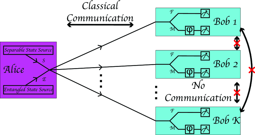
Figure 1: A protocol for estimating functions of quantum parameters held at multiple remote sites while maintaining security from eavesdropping and spoofing. In this scenario each Bob holds a parameter and Alice is attempting to estimate some linear function of these parameters. Each Bob can be trusted to follow Alice’s instructions but they are not guaranteed to be secure from observation. The Bobs do not need to be able to communicate with one other. Alice sends states that are entangled over all of the Bobs or an equal sized set of separable states to all of the Bobs in each round with probabilities $E$ and $S=1-E$ respectively. Each Bob chooses at random to interact the state they receive with their parameter or not with probabilities $M$ and $F=1-M$ respectively. Then they measure them and send the discrete measurement results to Alice through a public classical communication channel. Alice uses these results to verify for an eavesdropper and estimate the function of parameters.

The paper is structured as follows. In Section 2 we introduce our protocol and use Monte Carlo simulations to demonstrate the effectiveness of using separable or entangled initial states as well as a hybrid protocol. We consider two scenarios: 1. Alice performing a predetermined number of rounds and 2. Eve attacking every round by replacing the states in the quantum channel with her own entangled states until Alice detects her for the first time and stops the protocol. To maintain security we set a limit on the average information Eve can gain over many simulations and, within this limit, search for the optimal choice of parameters to maximise Alice’s estimation effectiveness. We show that entangled initial states are not effective for security as the number of Bobs increases whereas, separable initial states remain secure but have reduced measurement precision. Using a combination of both allows for both enhanced measurement precision and security.

In Sections 3 and 4 we investigate the information gain and information asymmetry of this protocol respectively. Section 3 begins by discussing Fisher information and why the asymptotic large data limit is difficult to reach in a secure network. Section 4 begins with an analytical calculation of the number of times Eve can successfully intercept information using attacks on the quantum and classical channels before she is detected. The sections then respectively show the information gain and asymmetry when using qubits and GHZ-like states to measure functions of phase parameters. In particular, we demonstrate the main result of this paper, which is that it is possible to simultaneously achieve network security and a measurement precision that surpasses the standard quantum limit.

2 Protocol

Our SQRS protocol proceeds as follows:

1. Alice prepares either an entangled state or a set of separable states with probabilities $E$ and $S$ respectively. These are chosen from a set that cannot be distinguished on a single shot and have occurrence probabilities such that the average state is proportional to the identity matrix. She keeps the state secret. The encoding for each member of the separable set is independent so, she does not send a set of identical separable states. When using qubits and GHZ states, the separable states sent to each Bob $b$ of the $B$ Bobs are each of the form

   $$\ket{S_{b}}=\left(\ket{0}+e^{i\chi_{b}}\ket{1}\right)/\sqrt{2}$$ (1)

   and the entangled states with an element sent to each Bob are

   $$\ket{E}=\left(\ket{0}^{\otimes B}+e^{i\chi}\ket{1}^{\otimes B}\right)/\sqrt{2}$$ (2)

   for B Bobs. For both types of initial state $\chi_{b},\chi\in\{\chi_{0},\chi_{0}+\pi/2,\chi_{0}+\pi,\chi_{0}+3\pi/2\}$ at random with equal probability for each state sent. For our purposes, the choice of $\chi_{0}$ is arbitrary so for the majority of our discussion, we take $\chi_{0}=0$ giving Pauli-X and Pauli-Y like states.

2. Alice sends the quantum states through a quantum communication channel to the Bobs with each receiving the state required for their individual parameter estimation. An eavesdropper could perform a spoof attack or the first step of a man in the middle attack here by measuring and replacing (or simply replacing) the probes in some or all of the rounds.

3. Each Bob independently, at random but with predetermined probabilities $M$ and $F$ either interacts their probe(s) with their parameter(s) or not respectively and then measures it. These measurements are performed in the $\chi_{0}$ and $\chi_{0}+\pi/2\}$ basis with equal probability (Pauli-X and Pauli-Y when $\chi_{0}=0$). Here, Eve could perform the second step of a man in the middle attack by observing the measurement results of the Bobs. The measurement probabilities are of the form $\frac{1}{2}(1+\cos(\varphi+k\pi/2))$ where $k\in\{0,1,2,3\}$ depends on the initial state and measurement basis and $\varphi$ is the sum of the parameters that measurement state has interacted with [11].

4. All the Bobs then communicate their measurement outcomes (along with whether they interacted the state with their parameter) to Alice through the public classical communication channel. Similar to stage 3 above, Eve could perform the second step of a man in the middle attack by observing the publicly announced results.

5. Alice is able to use the measurements from the Bobs along with her knowledge of the states she sent to perform an estimation of $\theta=\sum_{b=1}^{B}\phi_{b}$. As demonstrated previously [11], in this situation both the quantum and classical Fisher informations for and $\varphi$ being measured is 1. She is also able to continuously check for eavesdropping by looking for anomalies in the fidelity checking results where the Bobs did not interact the state with their parameter. She can then decide whether it is safe to continue the protocol, returning to step 1.

All SQRS protocols must find a way to balance both security and estimation efficiency. If we assume there is no eavesdropper, any protocol would be most efficient for measurements by having fidelity checking rate, $F=0$ and parameter measurement rate $M=1-F=1$. Similarly, the most secure protocol has $F=1$ and $M=0$. We choose $F$ to be equal for all Bobs and likewise for $M$, as this optimises the measurement efficiency and the security. This can be illustrated with the optimal measurement states for each Bob, $M_{b}$, occurring with rate proportional to $\prod_{j=1}^{B}M_{b}\leq M_{\text{mean}}^{B}$ with equality when all $M_{b}=M_{\text{mean}}$. Similarly, the optimal probability of fidelity checks for each Bob, $F_{b}$, can be found from $E\prod_{j=1}^{B}F_{b}+S\sum_{j=1}^{B}F_{b}\leq EF_{\text{mean}}^{B}+SBF_{\text{mean}}$ with equality when all $F_{b}=F_{\text{mean}}$ and thus all $M_{b}=M_{\text{mean}}$. Therefore, for the remainder of this article we use $F$ and $M$ as the same fidelity checking and parameter measurement probabilities for all Bobs.

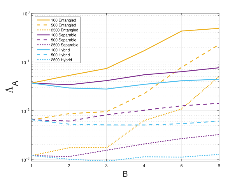
Figure 2: The mean, $\Lambda_{A}$ of Alice’s likelihood function circular mean square error, $\lambda(\vec{n},\vec{\phi})$ averaged over the sets of possible results $\vec{n}$ for many different values of Bobs’ phases $\vec{\phi}$ in situations where Eve’s mean circular mean square error has a lower bound $\Lambda_{E}\geq 1/2$ and minimised with respect to the protocol parameters $S$ and $F$ for a measure and replace with entangled states attack. This is plotted for three approaches: initial states entangled over all Bobs; initial states separable between the Bobs; hybrid of separable and entangled initial states used with probability of separable initial state $S$ for each round. Solid lines represent a maximum of 100 rounds, dashed lines for 500 rounds and dotted lines for 2500 rounds.

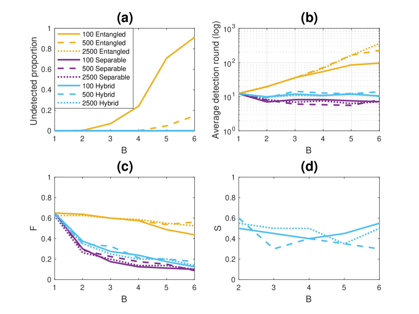
Figure 3: Optimisation results for $\Lambda_{E}\geq 0.5$ when Eve perform a measure and resend entangled state attack. (a)The proportion of times that Alice does not detect Eve before the end of the protocol. Other than 100 and 1 000 rounds entangled initial states, all of the lines are at or very close to zero and cannot be distinguished on this plot. (b) The number of rounds until Alice detects Eve for the first time. (c) Fidelity checking probabilities $F$. (d) Separable state probabilities $S$ for the hybrid protocol.

We performed Monte Carlo simulations under two different scenarios to demonstrate the effectiveness of our protocol in the low-data minimal prior information regime for estimating $\theta$ while maintaining security against an eavesdropper in man in the middle attacks where Eve intercepts the states that Alice sends, measures them and replaces them with corresponding entangled states. In the first scenario there is no eavesdropping, we calculate Alice’s likelihood function for $\theta$ given a set of results $\vec{n}$, $\mathcal{L}(\theta|\vec{n})$. Then calculate $\lambda(\vec{n},\vec{\phi})$, a circular analogue to the mean squared error of that likelihood function and average it over the results many simulations $\vec{n}(\vec{\phi})$ for many sets of true values, $\vec{\phi}$ to get a mean value $\Lambda$. We write this as $\Lambda_{A}$ for Alice and $\Lambda_{E}$ for Eve and $\Lambda$ when it could apply to both. $\lambda(\vec{n},\vec{\phi})$ is a measure of dispersion drawn from the measure of the distance between two angles $1-\cos(\hat{\theta}-\theta)$. It is defined as,

$$\lambda(\vec{n},\vec{\phi})=\int_{0}^{2\pi}\left(1-\cos(\hat{\theta}-\theta)\right)\mathcal{L}(\hat{\theta}|\vec{n})d\hat{\theta}=\frac{1}{2}MSE\left(\mathcal{L}\left(\theta|\vec{n}\right)\right)+\mathcal{O}\left(\left(\hat{\theta}-\theta\right)^{4}\right).$$ (3)

It is proportional to the cost function $C_{\theta,\hat{\theta}}=4\sin(\frac{\hat{\theta}-\theta}{2})$ used for limited data phase estimation with minimal prior information popular due to it being the simplest function that approximates the variance for small distribution [26]. This provides a useful measure where $\lambda(\vec{n},\vec{\phi})=0$ is a delta function around the true value, $\lambda(\vec{n},\vec{\phi})=1$ is a uniform distribution around $2\pi$, indicating no information in a circular sense and $\lambda(\vec{n},\vec{\phi})=2$ is a delta function around $\theta\pm\pi$ corresponding to the maximum possible error indicating measurement error or spoofing. Our circular data analysis techniques are further discussed in Appendix A.

In the second scenario Eve attacks every round measuring and replacing the states with her own states that are entangled over all Bobs and correspond to her measurement results. She continues to do this until Alice detects her the first time at which point the protocol is stopped. The security requirements are dependent on the specific scenario. Here we have chosen to limit $\Lambda_{E}\geq 0.5$, approximately equivalent to a linear mean squared error of at least 1. This gives Alice a guarantee on how little information Eve can gain. The limit put on $\Lambda_{E}$ can, of course, be varied depending on the scenario and application.

These two scenarios were chosen because the detection of Eve depends on the number of rounds that she attacks, not the number of rounds that Alice attempts. Also, to be sure that Eve could not get as much or more information than Alice, Alice would want to ensure that Eve is detected a long time before reaching the total number of rounds. If Alice reaches the total number of rounds intended and Eve attacks without being detected it should becasue she has only attacked a relatively small proportion of the rounds and thus cause only a small perturbation to Alice’s results. We attempt to minimise $\Lambda_{A}$ while ensuring $\Lambda_{E}\geq 0.5$ and that Eve is detected long before the end of the predetermined rounds. Details of the methodology can be found in Appendix B.

The results of these simulations for 100, 500 and 2500 rounds are shown in Fig. 2. They demonstrates that a hybrid of separable and entangled initial states outperforms the use of only one of the two, showing little variation in information gain with the number of Bobs. For the remainder of this section we will discuss these results in more detail while comparing them to Fig. 3 which shows (a) the rate of Eve going undetected, (b) the rounds until detection and (c,d) the protocol probabilities chosen by the optimisation algorithm. More detail on the information gain and security aspects can be found in Sections 3 and 4 respectively.

Entangled initial states are plotted in yellow (middle grey) on the figures. Fig. 2 demonstrates that this choice of Alice’s initial state performs increasingly worse than separable-only initial states and a hybrid protocol as the number of Bobs increases to the point that with low data and larger numbers of Bobs, Alice does little better than the security limits placed on Eve (i.e. $\Lambda\geq 0.5$). There are two issues with entangled initial states. The first is that, with limited data, it is difficult to gain much information for certain protocol parameters, further discussed in section 3. The second is that security reduces with the size of the network, further discussed in section 4.

For low data entangled only initial states performs even worse than Fig. 2 would suggest because the proportion of rounds where Eve goes undetected before the end of the protocols. The results shown in Fig. 2 do not account for Eve going undetected. Fig. 3(a) shows that 5 or more Bobs with 500 rounds and 3 or more Bobs with 100 rounds there is a non-negligible probability of Eve going undetected for the entire protocol. Firstly, this is unacceptable from a security point of view. Secondly, Fig. 3(b) demonstrates that this corresponds to an average number of rounds before detection being of the same order of magnitude as the total rounds. This means that the effect of an undetected eavesdropper (who may attack only some rounds) on Alice’s estimation would be more than a small amount of noise making her perform even worse than in Fig. 2 or forcing her to perform significantly more fidelity checks than Fig. 3(c) suggests which would also make her estimation even worse.

Separable initial states are plotted in dark purple (dark grey) on the figures. These show excellent security features regardless of the number of rounds. It can be seen in Fig. 3(b) that Alice’s optimised information gain is achieved while ensuring that Eve can attack fewer than 10 rounds on average before she is detected, independent of the number of rounds or number of Bobs. For separable states, the number of fidelity checks for a constant $F$ increases linearly with the number of Bobs so, as demonstrated in Fig. 3(c), $F$ can be reduced as the number of Bobs increases. However, the disadvantage of using separable initial states is that we miss out on the quantum enhanced measurement precision of entangled states. We see in Fig. 2 that this causes the measurement efficiency to reduce with the number of Bobs. The reduction is close to the linear reduction in a metrology protocol without security.

Hybrid initial states are plotted in light blue (light grey) on the figures. As the number of Bobs increases, the security is increasingly reliant on the separable initial states, Fig. 3(d). This is because the average number of security checks per round for entangled initial states is given by $F^{B}$ and so reduces rapidly with network size. By contrast, the average number of security checks per round for separable initial states increases with network size as $BF$ since there is the possibility of more than one check per round. The fidelity checking probability for hybrid initial states when optimised to fulfil security conditions and minimise Alice’s estimation dispersion is shown in Fig. 3(c) and follows a similar shape to the separable initial states. Similar to the separable only states, the average number of rounds before Eve is detected remains fairly low for any number of Bobs. It is not quite as low as the case of separable only states because, as shown in Fig. 3(d), many rounds make use of entangled states which have reduced security as discussed above. However, it remains sufficiently small that, in cases where Eve does not make enough attacks to be detected, we can approximate Alice’s information as that given by a protocol with no eavesdropper.

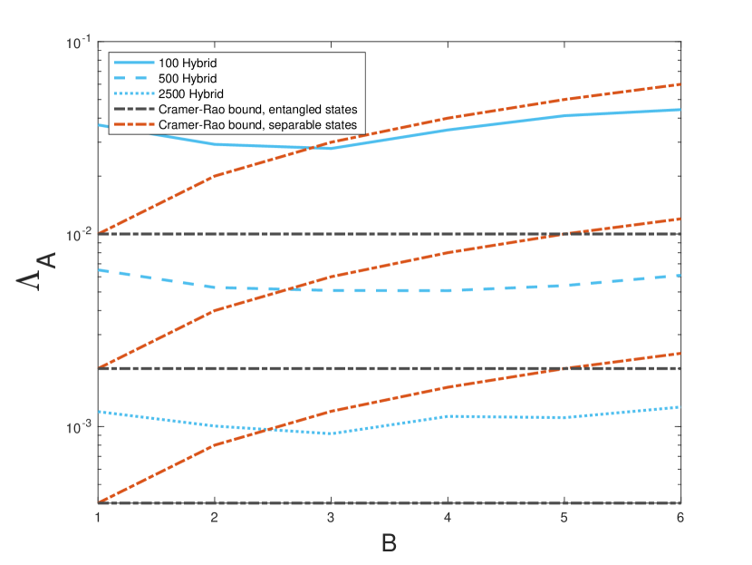
Figure 4: Comparison of Alice’s maximum $\Lambda_{A}$ while limiting Eve’s $\Lambda_{E}\geq 1/2$ with the Cramér-Rao bound for non-secured metrology protocols using separable and entangled probes.

The Cramér-Rao bounds for similar metrology protocols without security for separable and entangled initial states have variances given by $B/N$ and $1/N$ respectively, where $N$ is the number of rounds. When using hybrid initial states there is a trade-off between the enhanced security of separable states and enhanced measurement precision of entangled states. Fig. 4 shows that for three or more Bobs, the hybrid protocol (with $\Lambda_{E}\geq 0.5$) has an average dispersion less than the Cramér-Rao bound for separable probes and 3 or more Bobs. This shows quantum enhanced measurements and security combined into a single protocol.

3 Information gain in the asymptotic and low-data limits

The information Alice and Eve gain can be considered in the same way and depends on the number of rounds $N$ and the protocol parameters $B$, $S$ $(E=1-S)$ and $F$ $(M=1-E)$. The results in this section will be given in terms of these four independent parameters: $N$, $B$, $S$ and $F$. If Eve performs an attack where she replaces states with her own entangled or separable states then the results correspond to $S=0$ or $S=1$ respectively.

In a protocol with $B$ Bobs each measuring a parameter $\phi_{b}$, the set of combinations of Bobs that could perform parameter measurement or not in each round is of size $2^{B}$; there are $\binom{B}{m}$ combinations for $m$ parameters being measured. We write the set of possible combinations $\vec{\varphi}=\{0,\phi_{1},\phi_{2},...,\phi_{1}+\phi_{2},\phi_{1}+\phi_{3},...,\theta\}$ with each $\varphi_{k}(m)$ an element of $\vec{\varphi}$ with $m$ parameters measured. Appendix C demonstrates how the Fisher information of the protocol can be calculated by combining the information due to the sets of $\varphi_{k}(m)$ for each $m$. The probability of each $\varphi_{k}(m)$ being measured is

$$P_{k}(m)=SM\Big{|}_{m=1}+EM^{m}F^{B-m}.$$ (4)

Assuming that the Fisher information of each $\varphi_{k}(m)$ is the same for any given value of $m$, the Fisher information of the entire protocol relative to round total round count is

$$\mathcal{I}_{\text{total}}=\frac{SM\mathcal{I}_{1}}{B}+\sum_{m=1}^{B}EM^{m}F^{B-m}\frac{m}{B}\binom{B-1}{m-1}\mathcal{I}_{m},$$ (5)

where $\mathcal{I}_{m}$ denotes the classical Fisher information of each $\varphi_{k}(m)$. The same relationship also holds for the corresponding quantum Fisher information.

It is known that the quantum Cramér-Rao bound is valid only in the asymptotic limit of a large number of independent measurements [27, 28, 29, 30]. One condition of the asymptotic limit is that the maximum likelihood estimator becomes unbiased. It is important for our analysis to quantify when this limit is reached. For single qubit measurements, it has been shown there is an estimation bias of the maximum likelihood estimator for some values of the phase being estimated in limited data; as the amount of data increases that bias reduces and the range of values with non-negligible bias also reduces[11]. Similarly, the mean standard deviation of likelihood functions is at the Cramér-Rao bound for the same values of the phase where the bias is negligible[11]. Approximately $1000$ measurements is sufficient for both of these effects to affect only a small range of possible phases and by a reduced amount. Therefore, we use $1000$ measurements as an approximate asymptotic limit for any single $\varphi_{k}$ in this protocol[11].

To be able to combine estimators of $\varphi_{k}$ in the same way as the Fisher information of the system is calculated, each $\varphi_{k}$ must be measured in the asymptotic limit. The number of $\varphi_{k}$ increases exponentially with the number of Bobs $2^{B}$. Apart from the case of $E=0$ or $F=0$, these will all have a non-zero probability of occurring. If $E=1$ and $F=0.5$ they are all equally likely to occur, doing so at a rate of $2^{-B}$; for any other protocol parameters some will be even less likely. For all of them to be measured in the asymptotic limit at least $1000\times 2^{B}$ rounds are needed. Therefore, as the size of the network increases, more rounds are required for the Cramér-Rao bound to be valid.

We can almost reach the asymptotic limit if we consider that for some choices of system parameters the $\varphi_{k}(m)$ for some values of $m$ are very unlikely to occur. However, it is not advantageous to consider only the system parameters that reduce the number of $\varphi_{k}$ that need to be considered. For instance, taking $F=0.1$ or $F=0.9$ many of the $m$ are quite unlikely but they have low Fisher information and security respectively; while $0.1<F<0.9$ increases the number of $\varphi_{k}$ that need to be considered, if there are enough rounds it provides better information gain than $F=0.1$ and it always provides better security than $F=0.9$, so as demonstrated in Fig. 3(c) demonstrates that less extreme values of $F$ provide good balance between the two effects.

When the data is limited, and $\binom{B}{m}$ is large, it is not effective to perform parameter estimation of $\theta$ by combining all of the $\varphi_{k}(m)$ for each $m$ together. We can illustrate this by considering how the variance of the estimator of a random variable is inversely proportional to the number of measurements and the variance of an estimator of a sum of variables is equal to the sum of their variances. This means that the variance of the sum of parameters is limited by the parameter for which we have the least data. For example, if there are no data for one parameter and it has a $2\pi$ range uniform prior, as phases are circular, we gain no information about $\theta$ from all of the other results.

The number of results for all of the $\varphi_{k}$ is distributed as a multinomial and the marginal of each $\varphi_{k}$ is a binomial. When there are a lot of $\varphi_{k}(m)$ compared to the number of rounds the mean number of results for each is small and the standard deviation is large. This makes it inefficient to combine all $\binom{B}{m}$ to estimate $\binom{B-1}{m-1}\theta$ for limited data. Instead, we gain more information by combining those that have the most results and sum to some multiple of $\theta$. Our limited data parameter estimation methodology is further discussed in Appendix A.

In figure 5 we plot $\Lambda_{A}$ for 1, 2, 4 and 6 Bobs between 1 and 2500 rounds for protocols with no fidelity checking and either separable or entangled initial states only compared to the hybrid protocol as optimised for 2500 rounds. It clearly demonstrates that the hybrid protocol, while being secure, is also capable of performing quantum enhanced measurements for functions of parameters spread across a network of sensors with increasing effectiveness with network size. Using the values for $F$ and $S$ for the hybrid protocol optimised for 2500 rounds ensures that the protocols conform to the security limit up to 2500 rounds. However, it is not optimised for information gain with fewer rounds. This could be further enhanced by combinations of single and multiple pass estimations of $\theta$ set out for two-party SQRS [11].

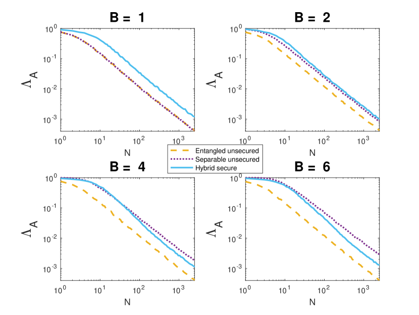
Figure 5: $\Lambda_{A}$ as a function of the number of rounds, $N$, for different protocols and different numbers of Bobs. The purple (dark grey) dotted line is the result for an non-secured ideal system using separable states. This represents the standard quantum limit which scales as $B/N$. The yellow (middle grey) dashed line shows the result for an unsecured ideal system using entangled states. This shows a Heisenberg scaling of $1/N$. The solid blue line (light grey) is the result for a system that uses a combination of separable and entangled initial states and is secure up to $N=2500$. The protocol parameters have been taken from Fig. 3 for $N=2500$. The information gain has not been optimised for fewer rounds but security is guaranteed.

4 Information asymmetry between Alice and Eve

Since our protocol has discrete detection results where Eve is either detected or not, we can model the number of rounds until Eve is detected using the geometric distribution. The probability that there are $\eta$ rounds before Eve is detected is given by,

$$P(\text{number of rounds before Eve is detected}=\eta|d)=(1-d)^{\eta}d$$ (6)

where $d$ is the probability that Eve will be detected in any given round. This can be used to model the amount of information gain for scenarios with a single Bob. Fig. 6 shows a lower limit on the amount of information gain for measure and resend attacks and replace attacks on a single Bob. This is also a demonstration of the security in a scenario where Eve attacks to gain information about the phase held by only one of the Bobs. This is calculated by using many Monte Carlo simulation to find $\Lambda$ for 0 to 100 rounds of the protocol then weighting this using the geometric distribution for the number of rounds before Eve is detected. When $F$ is very small, there is a non-negligible probability that more than 100 rounds can pass before Eve is detected. As stated in section 2, this already shows a failure of security. In these cases we set $\Lambda(\eta)=0$ making the plot a lower limit of $\Lambda_{E}$ for eavesdropping.

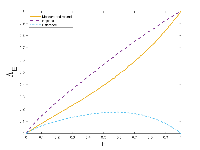
Figure 6: $\Lambda_{E}$ for a single-Bob protocol with measure and resend attacks and replace attacks. Data was created using simulations of $\Lambda(\eta)$ for $\eta=\{0,1,2,...100\}$ and combining them with the distribution of $\eta$ given by equation 6 with $d=F/8$ and $d=F/4$ respectively. For most values of $F$ the probability of being undetected in more than $100$ rounds is negligible meaning the values shown in this plot are the true values of $\Lambda_{E}$. For $F<0.1$ the probability is not negligible so the values shown in the plot represent a lower bound on $\Lambda_{E}$.

For a single Bob, the detection probability when Alice and Bob verify a qubit on which Eve has performed a measure and resend attack is $1/4$ [8, 11]. By a similar logic, when performing a replace attack the state on arrival is random giving a $1/2$ probability of Eve being detected. There are two measurement bases for the initial states and fidelity checks which all occur with equal probability so, there is a $1/2$ probability that Bob performs a fidelity check in the same basis as the initial state. Therefore, the detection probability for a single attacked round is $d(\text{measure and resend}|B=1)=F/8$ for measure and resend attacks and $d(\text{relpace}|B=1)=F/4$ for replace attacks. This can be generalised to allowing more than one detection using the negative binomial distribution.

For multiple Bobs we count the number of rounds including the one where Eve is detected. The probability of this is,

$$P(\text{number of rounds including when Eve is detected}=\eta|d)=(1-d)^{\eta-1}d.$$ (7)

If Alice only uses GHZ states, then the number of rounds that Eve gains information from, $\eta$, is distributed by equation 6. If Alice uses a separable state, the number of rounds that she gains information on can be described by either equation 6 or equation 7 depending on whether she gained any information from the final round. A separable state will have several independent tests and measurements and making it possible for Eve to gain some information as well as being detected one or more times in a single round. The maximum information gained for separable states is therefore bounded by what she would get from the number of rounds distributed by equations 6 and 7 from below and above respectively.

In a protocol using both separable and entangled initial states, we can model the upper limit on the number of rounds from which Eve gains information before she is detected $K$ times by combining the two geometric distributions into a special negative trinomial

$$P(\text{Eve's information gaining measurements until detected K times}\leq\eta|K,d_{S},d_{E})\leq\sum_{k=0}^{\min(\eta-1,K)}\binom{K}{k}u^{\eta-k}\,d_{S}^{k}\,d_{E}^{K-k},$$ (8)

where $u=1-d_{S}-d_{E}$ is the probability of being undetected in each round, $d_{E}$ and $d_{S}$ are respectively the probabilities of being detected from a separable or an entangled state in each round and $\eta$ is the number of measurements that Eve could have got results for before being detected. Similar to the single Bob case, this can be used with values of $\Lambda(\eta)$ to put a lower bound on $\Lambda_{E}$, an upper bound on Eve’s average information gain given the protocol parameters.

The detection probability depends both on the type of attack that Eve performs and the initial state. We take the probability that Eve is detected on a single measurement, when her strategy is to replace Alice’s state with a random one, as $d_{r}$. With initial entangled states, we need a coincidence of all the Bobs performing a fidelity check, $p=F^{B}$ and the net measurement to be in the same basis as the original state $p=1/2$ in order to detect Eve. The probability of this, $d_{E}$, is given by

$$d_{E}(\text{replace attack})=Ed_{r}F^{B}/2.$$ (9)

It is possible to detect Eve more than once in a single round when separable initial states are used. We are interested in the probability of there being at least one detection. For a replace attack the probability a detection by a single Bob is dependent on $d_{r}$, $F$ and the probability that the Bob performs the fidelity check in the same basis as the initials state $p=1/2$. So, for a replace attack, the probability of being detected from separable states at least once in a round is

$$d_{S}(\text{replace attack})=S\left(1-(1-d_{r}F/2)^{B}\right).$$ (10)

If Eve measures the quantum states and replaces them with her best guess at the same kind of state, the probability of her being detected, $d_{mr}$, in a fidelity check is less than it would have been if the replacement state was not informed by the measurement outcome, i.e. $d_{mr}\leq d_{r}$,

$$d_{S}(\text{measure and replace with separable}) =S\left(1-(1-d_{mr}F/2)^{B}\right)$$ (11)

$$d_{E}(\text{measure and replace with entangled}) =Ed_{mr}F^{B}/2.$$ (12)

If Eve measures an entangled state and replaces it with a separable state, when all of the Bobs perform a fidelity check Alice will interpret the state as if it was an entangled state. The net phase of the set of separable states sent by Eve would be the same as the phase if she had measured and replaced with an entangled state so the detection probability is the same

$$d_{E}(\text{measure and replace with separable})=Ed_{mr}F^{B}/2$$ (13)

If Eve measures a separable state and replaces it with an entangled state each Bob has an equal probability of getting a measurement result that corresponds to each of the initial states. The results are dependent on each other and the state that Eve sent but their distribution is the same for each Bob no matter the state Eve sent and no matter the initial state that Alice sent. Therefore, the detection probability is the same as a replace attack

$$d_{S}(\text{measure and replace with entangled})=S\left(1-(1-d_{r}F/2)^{B}\right)$$ (14)

Detection probability in each round
Eve attack type	separable initial state	entangled initial state
resend random separable	$S\left(1-(1-d_{r}F/2)^{B}\right)$	$Ed_{r}F^{B}/2$
resend random entangled	$S\left(1-(1-d_{r}F/2)^{B}\right)$	$Ed_{r}F^{B}/2$
measure and resend separable	$S\left(1-(1-d_{mr}F/2)^{B}\right)$	$Ed_{mr}F^{B}/2$
measure and resend entangled	$S\left(1-(1-d_{r}F/2)^{B}\right)$	$Ed_{mr}F^{B}/2$

Table 1: The probability of Eve being detected at least once in a round.

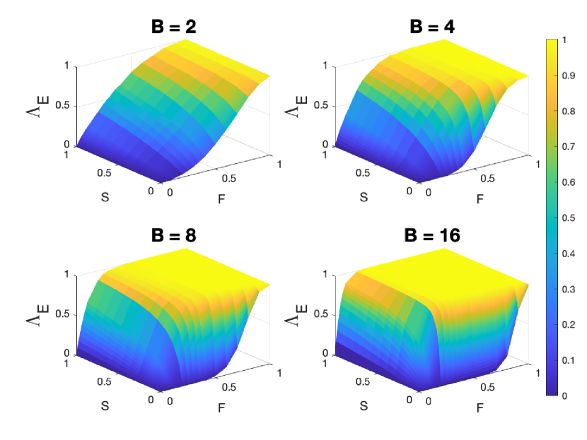
Figure 7: A lower limit on $\Lambda_{E}$ for 2, 4, 8 and 16 Bobs when performing a measure and replace with entangled state attack. The greater the value, the more secure the protocol.

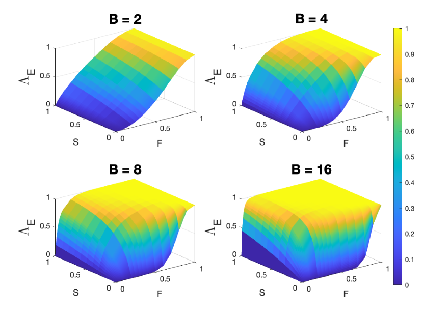
Figure 8: A lower limit on $\Lambda_{E}$ for 2, 4, 8 and 16 Bobs when performing a measure and replace with separable states attack. The greater the value, the more secure the protocol.

These probabilities are summarised in Table 1. As $d_{mr}\leq d_{r}$, it is clear that it is always advantageous for Eve to use a measure and resend attack rather than a replace attack. The detection probability is lower when replacing with a separable state than an entangled state but, the information gain is less. Therefore, it is not immediately obvious which attack is better for Eve. However, as the number of Bobs increases, a secure protocol increasingly relies on separable states for security, making the advantage of using measure and replace entangled over replace entangled reduce rapidly with the size of a secure network.

In our protocol Alice stops the first time she detects Eve. Substituting $K=1$ into equation 8, we get

$$P(\text{Eve's information gaining measurements until detected first time}=\eta|d_{S},d_{E})\leq u^{\eta-1}\Big{|}_{\eta\geq 1}\,d_{S}+u^{\eta}\,d_{E},$$ (15)

as a distribution that limits the number of rounds where Eve gains information before she is detected from above. Like the $B=1$ case, $d_{r}=1/2$ and $d_{mr}=1/4$. These, combined with the equations in Table 1 allow us to determine this distribution in terms of the system parameters. Similar to the single Bob scenario in Fig. 6, using Monte Carlo simulation to find $\Lambda(\eta)$ for $\eta\in\{0,1,2,...50\}$ and using a limiting value $\Lambda(\eta>50)\geq 0$ and weighting by the probability distribution of equation 15 to put a lower limit on $\Lambda_{E}$ for Eve’s attacks.

Figs. 7 and 8 show this lower limit for 2, 4, 8 and 16 Bobs for measure and resend entangled and separable states respectively. When deciding the parameters $S$ and $F$ for an implementation of the protocol Alice may choose a security limit $\Lambda_{E}$ then use any values on these plots that is greater than $\Lambda_{E}$ to get that level of security. If the intended number of rounds is very large the (inverse) Fisher information can be used to choose the optimal value. However, as discussed in section 3, the intricacies of limited data information gain in these scenarios mean that the Fisher information may not be appropriate and it may be better to use some other method to choose optimal values. Either results of optimisation algorithms such as those in section 2 can be used or, as the secure region is already determined, it suffices to perform a Monte Carlo simulation for the number of rounds Alice wants to use to determine a good choice of $S$ and $F$ selected from those values near the security limit calculated here.

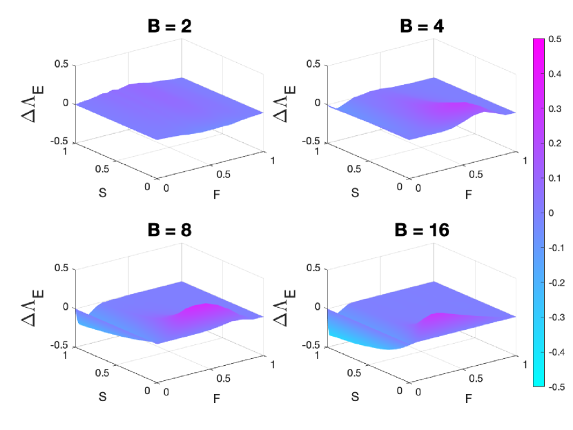
Figure 9: The difference in security between the two attacks in Figs. 7 and 8, $\Lambda_{E}$(entangled)$-\Lambda_{E}$(separable). The difference is negligible for the high security choices of S and F indicating that the choice of attack type makes little difference. With lower security S and F entangled attacks show an advantage for low fidelity while separable states show an advantage for low separable state probability. These differences increase with the number of Bobs.

5 Conclusion

We have demonstrated a method of performing quantum-enhanced metrology for functions of phase parameters at a collection of remote sites which is also secure from eavesdropping. The security persists even when the eavesdropper has access to the measurement results, the information in all classical communication channels and the ability to measure and manipulate states in quantum communication channels. Furthermore, we have demonstrated that the protocol can be made secure while achieving parameter estimation beyond the standard quantum limit for three or more Bobs.

We have demonstrated how the data can be analysed and the information gain quantified for both Alice, $\Lambda_{A}$, and Eve, $\Lambda_{E}$, with limited data. This is done by means of an analytical probability distribution for modelling the number of information gaining measurements Eve can get before being detected. This is used to put an upper limit on Eve’s information gain (lower limit on $\Lambda_{E}$) before she is detected and enables us to choose protocol parameters $S$ and $F$ to maximise Alice’s information gain (minimise $\Lambda_{A}$) for any desired level of security.

Our results show a way of implementing quantum enhanced sensing of functions of parameter over remote networks with information privacy. The performance could be further enhanced by using multipass schemes, quantum-encoded authentication and extended to security against joint attacks on both the classical and quantum channels [11]. The protocol may also be adapted to further metrology scenarios such as different prior distributions [27, 28, 29, 30], noisy scenarios [6, 5] and non-linear functions of parameters [22, 31].

6 Acknowledgements

We acknowledge financial support for this research from DSTL under Contract No. DSTLX1000146546.

7 Author declarations

The authors have no conflicts to disclose.

8 Data Availability

Matlab code for the production of data and its analysis is available at the github repository S-W-Moore.

Appendix A Data analysis

Linear statistics use a linear support whereas directional statistics, in general, are performed by considering each data point or point on a probability distribution as a vector in a higher dimensional space [32]. On a circle each data point can be represented by a vector, $\boldsymbol{x}$, parameterised by an angle, $\theta$

$$\boldsymbol{x}=(\cos(\theta),\sin(\theta))^{T},$$ (16)

or equivalently by a complex number

$$z=e^{i\theta}=\cos(\theta)+i\sin(\theta).$$ (17)

We calculate our likelihood functions, $\mathcal{L}(\varphi_{k})$, numerically using a grid approximation, by splitting the $2\pi$ support into $K=1024$ equally-sized bins such that $\theta_{k}=\theta_{0}+k/K,\ k\in\{0,1,2,...,K-1\}$ and calculating the value of the likelihood function for each bin.

We combine two or more likelihood functions to find the likelihood function of the sum of some of the $\varphi_{k}(m)$ (with the same $m$) parameters by convolving them using fast Fourier transforms. This reduces the order of operations for the convolution from $\mathcal{O}(K^{2})$ to $\mathcal{O}(K\log K)$ operations and can convolute as many likelihoods as we like in a single calculation providing further efficiency improvements. This produces likelihoods $\mathcal{L}(q\theta|\vec{n}),\ q\in\mathbb{N}^{+}$ from which we draw $\mathcal{L}(\theta|\vec{n})$. We do this for all of the $\varphi_{k}$ for which we have enough data then take the product of all the $\mathcal{L}(\theta|\vec{n})$ and normalise to get a final normalised likelihood function for the protocol.

Drawn from the distance between two angles $1-\cos(\beta-\alpha)$ measure of circular dispersion [32] for some circular measurement data or distribution $\vec{\beta}$ around some point $\alpha$ is

$$D(\alpha)=\frac{1}{M}\sum_{m=1}^{M}\{1-\cos(\beta_{m}-\alpha)\}.$$ (18)

From a Bayesian perspective, the posterior distribution given by Bayes’ rule,

$$p(\theta|\vec{n},\alpha)\propto\mathcal{L}(\theta|\vec{n},\alpha)p(\theta|\alpha),$$ (19)

is the probability distribution of the parameter $\theta$ given the measurement data $\vec{n}$ and a prior distribution $p(\theta|\alpha)$ where $\alpha$ is the prior distribution’s hyperparameters (sometimes ommited when writing the posterior distribution alone). For this article we have used a uniform prior distribution $p(\theta|\alpha)=\frac{1}{2\pi}$ over an arbitrary $2\pi$ range. Therefore, the posterior distribution is equal to the normalised likelihood function. This broad prior with limited data creates broad posterior distributions which requires that we use allows us to make a circular analogue to the mean square error. We get this from the circular dispersion around the true parameter value $D(\theta)$ to the grid approximation of the likelihood function in equation 3 to get $\lambda(\vec{n},\vec{\phi})=\int D(\theta)d\mathcal{L}(\theta|\vec{n})$. When this is averaged over many sets of data for a set of input parameters it gives $\Lambda$ as a measure of information gain for those parameters.

While logical to combine all $\binom{B}{m}$ parameters $\varphi_{k}(m)$ that have the same $m$ to get $\binom{B-1}{m-1}$, like we do to calculate the Fisher information, it is advantageous both from a numerical efficiency standpoint and a limited data analysis perspective to take a more refined approach. An extreme example is when there is no data for one $\varphi_{k}(m)$ then it has a uniform distribution, like its prior and it’s circular convolution with any other circular distribution is also uniform. This can render the information for all of the parameters we are attempting to combine with this no-data parameter useless for estimating $\theta$.

As explained in section 3, in limited data the number of results for each $\varphi_{k}(m)$ varies enough that it worth accounting for the variance of the combination of independent $J$ variables, $X_{j}$,

$$Var\left(\sum_{j=1}^{J}X_{j}\right)=\sum_{j=1}^{J}Var\left(X_{j}\right)=c\sum_{j=1}^{J}\frac{1}{n_{j}},$$ (20)

for some constant c. We may use this principle as to create a figure of merit,

$$n_{\text{effective}}=\left(\sum_{j=1}^{J}\frac{1}{n_{j}}\right)^{-1}$$ (21)

for limited data analysis. If any $n_{j}=0$ then $n_{eff}=0.$ To optimise the information gain we make a list of all of the possible combinations of the $\varphi_{k}(m)$ with the same $m$ that sum to the smallest possible integer multiple of $\theta$ and search for the way of combining them that maximises the sum of the $n_{eff}$ and use those sets of combinations to estimate the likelihood function. The number of possible combinations increases rapidly with the number of Bobs, in particular when $m\approx B/2$. Therefore, to improve computation speed for larger numbers of Bobs (eg 16) when the number of combinations is very large we perform the optimisation for the $\varphi_{k}(m)$ with the largest $n_{j}$, record the best combinations, add the next largest to the remaining set and repeat until no non-zero data combinations are available.

Appendix B Optimisation algorithm

We found the minimum dispersion for Alice given the security conditions and round count by searching through the possible protocol parameters. First, for $B=\{1,2,3,4,5,6\}$ Bobs and $N=\{100,500,2500\}$ rounds an evenly spaced $11\times 11$ grid of possible $S$ and $F$ in the range $[0,1]$, we performed the simulations of Alice’s information gain for N rounds and Alice’s information gain until the first time she is detected 16 times for 64 sets of B randomly chosen parameters (the same set for all simulations for $\{B,N\}$). We calculated $\mathcal{L}(\theta|\vec{n})$ for each set of results and took the average for every grid point to find $\Lambda_{A}$ and $\Lambda_{E}$ at that point in that grid.

Figs. 7 and 8 demonstrate the security is monotonic in both $F$ and $S$ for each $B$. The Fisher information is also monotonic in the opposite direction. However, as demonstrated in section 3 the limited data information gain is not necessarily monotonic. Due to this, we devised an optimisation algorithm where we find the positions in each grid direction where the security condition $\Lambda_{E}\geq 0.5$ is met and $\Lambda_{A}$ is minimised for each $S$. Then, we build a new, evenly spaced, grid with half the spacing of the previous grid out of those points and all of the points between them and repeated the previous step. We repeated the optimisation step 3 times and used the results of the simulations for the single grid point that minimised $\Lambda_{A}$ while $\Lambda_{E}\geq 0.5$ for each $\{B,N\}$ to make the plots in section 2.

We created Fig. 5 by taking the best optimised values $\{S,F\}$ for $B=\{1,2,4,6\}$ and calculating $\Lambda_{A}$ for $100$ values in the range $[1,2500]$ by using the same simulations for Alice and plotting them against similar simulations with $F=0$ and either $S=0$ or $S=1$.

Appendix C Fisher information of protocol

When calculating the Fisher information for the whole protocol relative to the number of rounds we use the probability of each $\varphi_{k}$ occurring. The following calculation will use $\mathcal{I}_{m}$ for the Fisher information, both classical and quantum when m parameters are measured together. First, considering the (quantum) Fisher information in a protocol using only separable initial states. Each Bob has a probability $M$ of performing a parameter estimation. Therefore, measurements of each of the $\phi_{b}$ will occur with a probability of M per round. Measuring each parameter separately and summing them to get an estimation for $\theta=\sum_{b=1}^{B}\phi_{b}$ gives a (quantum) Fisher information

$$\mathcal{I}(\theta|\text{separable only protocol})=\frac{M\mathcal{I}_{1}}{B}.$$ (22)

If the protocol has a mix of states, the information gain due to separable states would be weighted by the probability of a separable initial state occurring

$$\mathcal{I}(\theta,S)=\frac{SM\mathcal{I}_{1}}{B}.$$ (23)

When considering entangled initial states, the probability of each sum of $m$ parameters $\varphi_{k}(m),k\in\{1,2,...,\binom{B}{m}\}$ being measured is equal. Therefore, it is practical to combine them to find the (quantum) Fisher information due to all of those parameters. They each have an equal probability

$$P(m,k|B,F,E)=EM^{m}F^{B-m}$$ (24)

of occurring. Their sum is

$$\sum_{k=1}^{\binom{B}{m}}\varphi_{k}(m)=\binom{B-1}{m-1}\theta.$$ (25)

This is evident by considering choosing only and all those combinations that contain an arbitrarily specific parameter there remain m-1 parameters to pick out of a remaining set of B-1. Therefore, $\binom{B-1}{m-1}$ combinations contain each parameter and so the sum of all of them contains the same multiple of that parameter. The (quantum) Fisher information for a single measurement follows the relationship

$$\mathcal{I}(aX)=a^{2}\mathcal{I}(X),$$ (26)

and (quantum) Fisher information due to an equally probable set of A states that sum to aX is

$$\mathcal{I}(aX)=a^{2}\mathcal{I}(X)/A.$$ (27)

Therefore, the (quantum) Fisher information from the $\binom{B}{m}$ sums of m of the B parameters have a Fisher information

$$\mathcal{I}(\theta|\text{entangled, m parameters in a round})=\frac{\binom{B-1}{m-1}^{2}}{\binom{B}{m}}\mathcal{I}_{m}=\frac{m}{B}\binom{B-1}{m-1}\mathcal{I}_{m}.$$ (28)

Combined with the occurrence probability of each individual state, this contributes

$$\mathcal{I}(\theta,E,m)=EM^{m}F^{B-m}\frac{m}{B}\binom{B-1}{m-1}\mathcal{I}_{m}.$$ (29)

The (quantum) Fisher information combines additively so, for independent data X and Y

$$\mathcal{I}_{X,Y}(\theta)=\mathcal{I}_{X}(\theta)+\mathcal{I}_{Y}(\theta).$$ (30)

Therefore, the (quantum) Fisher information for the entire system relative to the number of rounds may be found by adding the information from equations 23 and 29 for $m=1,2,...B$,

$$\mathcal{I}_{\text{total}}=\frac{SM\mathcal{I}_{1}}{B}+\sum_{m=1}^{B}EM^{m}F^{B-m}\frac{m}{B}\binom{B-1}{m-1}\mathcal{I}_{m}.$$ (31)

The probability of each $\varphi_{k}$ occurring is dependent only on the number of parameters measured $m$,

$$P_{k}(m)=SM\Big{|}_{m=1}+EM^{m}F^{B-m}.$$ (32)

References

- [1] Vittorio Giovannetti, Seth Lloyd and Lorenzo Maccone “Positioning and clock synchronization through entanglement” In Phys. Rev. A 65 American Physical Society, 2002, pp. 022309 DOI: 10.1103/PhysRevA.65.022309
- [2] P. Kómár et al. “A quantum network of clocks” In Nature Physics 10.8, 2014, pp. 582–587 DOI: 10.1038/nphys3000
- [3] Hiroto Kasai et al. “Anonymous Quantum Sensing” In Journal of the Physical Society of Japan 91.7, 2022, pp. 074005 DOI: 10.7566/JPSJ.91.074005
- [4] Yuki Takeuchi et al. “Quantum remote sensing with asymmetric information gain” In Phys. Rev. A 99 American Physical Society, 2019, pp. 022325 DOI: 10.1103/PhysRevA.99.022325
- [5] Hideaki Okane et al. “Quantum remote sensing under the effect of dephasing” In Phys. Rev. A 104 American Physical Society, 2021, pp. 062610 DOI: 10.1103/PhysRevA.104.062610
- [6] Peng Yin et al. “Experimental Demonstration of Secure Quantum Remote Sensing” In Phys. Rev. Applied 14 American Physical Society, 2020, pp. 014065 DOI: 10.1103/PhysRevApplied.14.014065
- [7] Nathan Shettell, Majid Hassani and Damian Markham “Private network parameter estimation with quantum sensors”, 2022 DOI: 10.48550/arXiv.2207.14450
- [8] Zixin Huang, Chiara Macchiavello and Lorenzo Maccone “Cryptographic quantum metrology” In Phys. Rev. A 99 American Physical Society, 2019, pp. 022314 DOI: 10.1103/PhysRevA.99.022314
- [9] Dong Xie, Chunling Xu, Jianyong Chen and An Min Wang “High-dimensional cryptographic quantum parameter estimation” In Quantum Information Processing 17.5, 2018, pp. 116 DOI: 10.1007/s11128-018-1884-z
- [10] Nathan Shettell, Elham Kashefi and Damian Markham “Cryptographic approach to quantum metrology” In Phys. Rev. A 105 American Physical Society, 2022, pp. L010401 DOI: 10.1103/PhysRevA.105.L010401
- [11] Sean W. Moore and Jacob A. Dunningham “Secure quantum remote sensing without entanglement” In AVS Quantum Science 5.1, 2023, pp. 014406 DOI: 10.1116/5.0137260
- [12] Vittorio Giovannetti, Seth Lloyd and Lorenzo Maccone “Advances in quantum metrology” In Nature Photonics 5.4, 2011, pp. 222–229 DOI: 10.1038/nphoton.2011.35
- [13] Luca Pezzé et al. “Optimal Measurements for Simultaneous Quantum Estimation of Multiple Phases” In Physical Review Letters 119, 2017 DOI: 10.1103/PhysRevLett.119.130504
- [14] Luca Pezzè “Entanglement-enhanced sensor networks” In Nature Photonics 15.2, 2021, pp. 74–76 DOI: 10.1038/s41566-020-00755-x
- [15] Xueshi Guo et al. “Distributed quantum sensing in a continuous-variable entangled network” In Nature Physics 16.3, 2020, pp. 281–284 DOI: 10.1038/s41567-019-0743-x
- [16] P.. Knott et al. “Local versus global strategies in multiparameter estimation” In Physical Review A American Physical Society, 2016 URL: https://journals.aps.org/pra/abstract/10.1103/PhysRevA.94.062312
- [17] T.. Proctor, P.. Knott and J.. Dunningham “Networked quantum sensing”, 2017 arXiv:1702.04271 [quant-ph]
- [18] Timothy J. Proctor, Paul A. Knott and Jacob A. Dunningham “Multiparameter estimation in networked quantum sensors” In Physical Review Letters American Physical Society, 2018 URL: https://journals.aps.org/prl/abstract/10.1103/PhysRevLett.120.080501
- [19] Jesús Rubio, Paul A Knott, Timothy J Proctor and Jacob A Dunningham “Quantum sensing networks for the estimation of linear functions” In Journal of Physics A: Mathematical and Theoretical 53.34 IOP Publishing, 2020, pp. 344001 DOI: 10.1088/1751-8121/ab9d46
- [20] Zachary Eldredge et al. “Optimal and secure measurement protocols for Quantum Sensor Networks” In Physical Review A American Physical Society, 2018 URL: https://journals.aps.org/pra/abstract/10.1103/PhysRevA.97.042337
- [21] Wenchao Ge et al. “Distributed quantum metrology with linear networks and separable inputs” In Physical Review Letters American Physical Society, 2018 URL: https://journals.aps.org/prl/abstract/10.1103/PhysRevLett.121.043604
- [22] Kevin Qian et al. “Heisenberg-scaling measurement protocol for analytic functions with Quantum Sensor Networks” In Physical Review A American Physical Society, 2019 URL: https://journals.aps.org/pra/abstract/10.1103/PhysRevA.100.042304
- [23] Timothy Qian et al. “Optimal measurement of field properties with quantum sensor networks” In Phys. Rev. A 103 American Physical Society, 2021, pp. L030601 DOI: 10.1103/PhysRevA.103.L030601
- [24] Jacob Bringewatt et al. “Protocols for estimating multiple functions with quantum sensor networks: Geometry and performance” In Phys. Rev. Res. 3 American Physical Society, 2021, pp. 033011 DOI: 10.1103/PhysRevResearch.3.033011
- [25] Jacob Bringewatt, Adam Ehrenberg, Tarushii Goel and Alexey V. Gorshkov “Optimal function estimation with photonic quantum sensor networks” In Phys. Rev. Res. 6 American Physical Society, 2024, pp. 013246 DOI: 10.1103/PhysRevResearch.6.013246
- [26] Rafał Demkowicz-Dobrzański “Optimal phase estimation with arbitrary a priori knowledge” In Phys. Rev. A 83, 2011 DOI: 10.1103/PhysRevA.83.061802
- [27] Jesús Rubio, Paul Knott and Jacob Dunningham “Non-asymptotic analysis of quantum metrology protocols beyond the Cramér–Rao bound” In Journal of Physics Communications 2.1 IOP Publishing, 2018, pp. 015027 DOI: 10.1088/2399-6528/aaa234
- [28] Jesús Rubio and Jacob Dunningham “Quantum metrology in the presence of limited data” In New Journal of Physics 21.4 IOP Publishing, 2019, pp. 043037 DOI: 10.1088/1367-2630/ab098b
- [29] Jesús Rubio and Jacob Dunningham “Bayesian multiparameter quantum metrology with limited data” In Phys. Rev. A 101 American Physical Society, 2020, pp. 032114 DOI: 10.1103/PhysRevA.101.032114
- [30] Jasminder Sidhu and Pieter Kok “Geometric perspective on quantum parameter estimation” In AVS Quantum Science 2, 2020, pp. 014701 DOI: 10.1116/1.5119961
- [31] Mauro Valeri et al. “Experimental adaptive Bayesian estimation of multiple phases with limited data” In npj Quantum Information 6.1, 2020, pp. 92 DOI: 10.1038/s41534-020-00326-6
- [32] Kanti V Mardia and Peter E Jupp “Directional Statistics”, Wiley Series in Probability and Statistics Chichester, England: John Wiley & Sons, 1999