Preserving quantum information in $f(Q)$ cosmology

Abstract

The effects of cosmological expansion on quantum bosonic states are investigated, using quantum information theory. In particular, a generic Bogoliubov transformation of bosonic field modes is considered and the state change on a single mode is regarded as the effect of a quantum channel. Properties and capacities of this channel are thus explored in the framework of $f(Q)$ theories. As immediate result, we obtain that the information on a single-mode state appears better preserved, whenever the number of particles produced by the cosmological expansion is small. Hence, similarly to general relativity, we show that analogous particle productions result even if we consider symmetric teleparallel gravity theories. Thus, we investigate a power law $f(Q)$ model, leaving unaltered the effective gravitational coupling, and minimise the corresponding particle production. We thus show how to optimise the preservation of classical and quantum information, stored in a bosonic mode states in the remote past. Finally, we compare our findings with those obtained in general relativity.

I Introduction

Data storage is intimately related to the preservation of information contained in a given set of data [1]. A fundamental objective in information storage is ensuring its long-term preservation [2, 3]. To reach this goal, one faces limitations dictated by physical theories [4]. Recently, those limitations have stemmed from the natural expansion of the universe [5, 6], which can introduce inevitable effects on any physical system as due to the gravitational theory that induces the expansion itself [7, 8].

To better explain how this works, it is required a comprehensive framework that combines both the underlying gravitational theory and quantum information. This may be provided by relativistic quantum information theory [9], i.e., a treatment that explores a wide range of topics involving the matching of quantum mechanics and general relativity (GR) in communication scenarios, addressing, for example, the problem of causal signaling [10, 11], of black hole information paradox [12, 13, 14], of gravity-induced entanglement [15, 16] and of analogue gravity systems [17, 18].

The scope of relativistic quantum information extends to weak gravitational limits, where it examines communication through quantum fields within curved spacetimes [19, 20, 21, 22]. Among the most prevalent applications are particle detector models, which represent non-relativistic quantum systems interacting with quantum fields [23, 24, 25]. These models offer a realistic framework for investigating communication between distant quantum detectors within a diverse range of background spacetimes and trajectories [26, 27, 28, 29].

Similarly, one can explore communication in curved spacetimes by tracing the evolution of bosonic or fermionic states from the remote past to the distant future using Bogoliubov transformations [19]. This approach is considered both realistic and effective, especially when assessing the preservation of information over extended time intervals [30, 31, 32, 33]. Further, this communication scenario can be seen as the communication between two particle detector models interacting with the field via the Jaynes-Cummings Hamiltonian [34, 35].

A specific inquiry, addressing the preservation of information stored in the distant past under the backdrop of cosmological expansion, particularly in the context of fermions, has been recently discussed [31]. In particular, it was proved that the cosmological particle production [36] is responsible for the damping of a remote past signal. Moreover, the cosmological particle production are the main source of the cosmological entanglement, carrying quantum correlations from the remote past [37, 38, 39]. For all these reasons, the particles produced by the expanding universe are expected to have a fundamental role in the storage of classical and quantum information from the remote past, even if encoded in bosonic systems [40].

On the other side, the remarkable success of GR has led to insights into our understanding of the universe [41]. Although the theory is elegant, well passing current observations, there is a theoretical and speculative need for those models extending or modifying Einstein’s theory [42, 43, 44, 45]. This is crucial for shedding light on potential effects that might manifest in regions of intense gravitational forces where Einstein’s theory is thought to break down [46, 47] or in cosmology, where dark energy and dark matter are currently open challenges [48, 49].

Among all, a recent theory describing the large scale universe has been employed by virtue of violating the metricity postulate on the metric [50]. Classes of such theories, named symmetric teleparallel gravity (STEGR), in particular the so called $f(Q)$ gravity [51, 52, 53], represent attempts entering the so-called trinity of gravity [54, 55], where alternatives to Einstein’s theory aim to describe the universe without passing through the concept of curvature. In this respect, promising examples of $f(Q)$ models have been considered in astrophysics [56, 57], gravitation sector [58, 59] and cosmology [60, 61, 62, 63], matching several astronomical observations without involving any form of dark energy [64, 65].

Motivated by preserving information and developing alternatives to Einstein’s gravity, we here investigate preservation of information stored in bosons within the context of $f(Q)$ gravity. In so doing, we study the evolution of bosonic Gaussian states from remote past to far future using Bogoliubov transformation. We show that the rate of classical and quantum information is compromised by the cosmological particle production for bosons. Hence, we seek for the minimization of particle production proving that the latter represents the optimal scenario for preservation of information stored in remote past. To this aim, we consider modifications of STEGR, wondering if these could better preserve information, stored in bosonic states. Hence, by imposing an appropriate Yukawa-like non-minimal coupling between the phion field and the non-metricity, we find the corresponding rate of particle production. To do so, we specialize our background adopting the Bernard-Duncan scale factor, having the advantage of being flat at past and future regimes. Afterwards, using a precise power law scenario for $f(Q)$, we bound the corresponding free parameters, optimizing the preservation of information from the remote past, indicating how suitable $f(Q)$ theories may be built up. Accordingly, our outcomes are compared with previous findings, checking possible similarities with both the fermionic case and particles produced in pure GR.

The paper is organized as follows. In Sec. II, we study the communication of bosonic Gaussian states under Bogoliubov transformations, focusing on a single mode. The classical and quantum capacity of the quantum channel arising from these transformations is found as well. In Sec. III, we include the universe expansion and see the role of particles produced on the evolution of bosonic single-mode states. In Sec. IV, we develop a perturbative approach to study the particle production in STEGR and its $f(Q)$ generalization showing how gravity modifications could increase or decrease it. A specific example is provided. Discussion, conclusions and perspectives are reported in Sec. VI.

II Evolution of Gaussian states through Bogoliubov transformations

Let us examine how a particular class of bosonic states, i.e. Gaussian states, undergoes transformation when subjected to a Bogoliubov transformation. In the context of quantum field theory in curved spacetime, an evolving metric, in the distant past up to the infinite future, involves a Bogoliubov transformation of the normal modes of the bosonic field [19, 23, 20]. As a result, we begin by defining bosonic Gaussian states and exploring their properties. Subsequently, we delve into the transformation of these states under Bogoliubov transformations and we finally examine the properties of a general quantum channel, constructed by the Bogoliubov transformations.

II.1 Bosonic Gaussian states

Among bosonic states, we single out bosonic Gaussian states (BGS), being of paramount importance in continuous variable quantum information theory [40]. We assume possible momenta and the fact that bosons can form a discrete set of cardinality $N$. We then label each of them with a subscript $i=1\ldots N$.

The expansion of a scalar field $\hat{\Phi}$ into normal modes reads [19]

$$\hat{\Phi}=\sum_{i=1}^{N}\left(a_{i}\phi_{i}+a_{i}^{\dagger}\phi_{i}^{\ast}\right)\,,$$ (1)

where $a_{\mathbf{i}}$ is the annihilation operator associated with a particle with momentum $i$, satisfying the bosonic algebra

$$\left[a_{i},a^{\dagger}_{j}\right]=\delta_{ij},\quad\left[a_{i},a_{j}\right]=0\,.$$ (2)

The set of normal modes $\{\phi_{i}\}_{i=1}^{N}$ in Eq. (1) has to be complete and orthogonal with respect to the scalar product $\left(\phi_{1},\phi_{2}\right)$ defined as

$$(\phi_{1},\phi_{2}) =-i\int_{\Sigma}\phi_{1}(x)\overleftrightarrow{\partial_{t}}\phi_{2}^{\ast}(x)d\Sigma$$

$$\coloneqq-i\int_{\Sigma}\left(\phi_{1}(x)\partial_{t}\phi_{2}^{\ast}(x)-(\partial_{t}\phi_{1}(x))\phi_{2}^{\ast}(x)\right)d\Sigma\,,$$ (3)

where $\Sigma$ is a Cauchy surface for the background spacetime of the field.

An $N$-mode BGS is entirely characterized by two elements:

• the first momentum vector $\mathbf{d}=(d_{1},\dots,d_{N})$, with $d_{i}=\left(\langle Q_{i}\rangle,\langle P_{i}\rangle\right)$,

• the covariance matrix:

  $$\sigma=\left(\begin{array}[]{c|c|c}\sigma_{11}&\dots&\sigma_{1N}\\ \hline\cr\vdots&\ddots&\vdots\\ \hline\cr\sigma_{N1}&\dots&\sigma_{NN}\end{array}\right)\,,$$ (4)

  where

  $$\sigma_{ij}=\frac{1}{2}\left(\begin{matrix}\langle\left\{Q_{i},Q_{j}\right\}\rangle-2\langle Q_{i}\rangle\langle Q_{j}\rangle&\langle\left\{Q_{i},P_{j}\right\}\rangle-2\langle Q_{i}\rangle\langle P_{j}\rangle\\ \langle\left\{P_{i},Q_{j}\right\}\rangle-2\langle P_{i}\rangle\langle Q_{j}\rangle&\langle\left\{P_{i},P_{j}\right\}\rangle-2\langle P_{i}\rangle\langle P_{j}\rangle\end{matrix}\right).$$ (5)

Here,

$$Q_{i}=\frac{1}{\sqrt{2}}\left(a_{i}^{\dagger}+a_{i}\right)\,,\quad P_{i}=\frac{1}{i\sqrt{2}}\left(a_{i}-a_{i}^{\dagger}\right)\,,$$ (6)

are called quadrature operators, satisfying $\left[Q_{i},P_{j}\right]=i\delta_{ij}$. Moreover, in Eq. (5), $\langle\cdot\rangle$ indicates the expectation value of the operator $\cdot$ in the bosonic state.

As entropic quantities are independent of the first momentum vector [66], we set $\mathbf{d}=\mathbf{0}$ for simplicity, having for the submatrices $\sigma_{ij}$ of $\sigma$, described in Eq. (5),

$$\sigma_{ij}=\frac{1}{2}\left(\begin{matrix}\langle\left\{Q_{i},Q_{j}\right\}\rangle&\langle\left\{Q_{i},P_{j}\right\}\rangle\\ \langle\left\{P_{i},Q_{j}\right\}\rangle&\langle\left\{P_{i},P_{j}\right\}\rangle\end{matrix}\right)\,.$$ (7)

The submatrices $\sigma_{ii}$, in diagonal blocks from the $\sigma$ matrix of Eq. (4), represent the reduced states of the various modes and, so, from Eq. (7), expanding the quadrature operators and using the algebra (2), each submatrix $\sigma_{ii}$ can be rewritten as

$$\sigma_{ii}=\left(\begin{matrix}\frac{1}{2}+n_{i}+\real m_{i}&\imaginary m_{i}\\ \imaginary m_{i}&\frac{1}{2}+n_{i}-\real m_{i}\end{matrix}\right)\,,$$ (8)

where $n_{i}\coloneqq\langle a^{\dagger}_{i}a_{i}\rangle$, i.e., the expectation value of particle number in the mode $i$, and $m_{i}\coloneqq\langle a_{i}a_{i}\rangle$. In this regards, the absolute value of $m_{i}$ is bounded between $0$ and $\sqrt{n_{i}(n_{i}+1)}$ - generating a thermal state and a squeezed vacuum state, respectively.

Conversely, the matrices $\sigma_{i\neq j}$ in the off-diagonal blocks of $\sigma$ represent the correlation between modes $i$ and $j$, so, following the above same procedure, these matrices turn into

$$\sigma_{i\neq j}=\left(\begin{matrix}\real\gamma_{ij}+\real\chi_{ij}&\imaginary\gamma_{ij}+\imaginary\chi_{ij}\\ -\imaginary\gamma_{ij}+\imaginary\chi_{ij}&\real\gamma_{ij}-\real\chi_{ij}\end{matrix}\right)\,,$$ (9)

where $\gamma_{ij}=\langle a_{i}^{\dagger}a_{j}\rangle$, $\chi_{ij}=\langle a_{i}a_{j}\rangle$.

Then, the parameters defining a $N$-mode Gaussian states become $n_{i}\in\mathbb{R}$, $m_{i},\gamma_{ij},\chi_{ij}\in\mathbb{C}$, with $i,j=1,\dots,N$.

If the modes $i=1,\dots,N$ are not correlated, i.e., $\gamma_{ij}=\chi_{ij}=0$, the covariance matrix $\sigma$, Eq. (4), leads to $\sigma=\bigoplus_{i=1}^{n}\sigma_{ii}$. Moreover, a vacuum state is given by $n_{i}=m_{i}=\gamma_{ij}=\chi_{ij}=0$, yielding $\sigma=\frac{1}{2}\mathbb{I}_{2N\times 2N}$.

II.2 Bogoliubov transformation

We here investigate the impact of a Bogoliubov transformation on a bosonic Gaussian state as the background spacetime evolves over time, transitioning from remote past to far future, where a static metric is assumed in both of these limiting regions.

In general, the modes at far future (or output modes) $\{\phi_{i}^{out}\}_{i=1}^{N^{\prime}}$ and the ones at remote past (or input modes) $\{\phi_{i}^{in}\}_{i=1}^{N}$ are different. Remarkably at the far future, new modes may emerge and, accordingly, the total number of modes, which was originally denoted as $N$, now becomes $N^{\prime}$. Both sets $\{\phi_{i}^{in}\}_{i=1}^{N}$ and $\{\phi_{i}^{out}\}_{i=1}^{N^{\prime}}$ consist of complete sets of orthonormal modes.

From this fact, each output mode can be written in terms of the input ones through the completeness relation

$$\phi_{i}^{out}=\sum_{j=1}^{N}\left(\alpha_{ij}\phi_{j}^{in}+\beta_{ij}\phi_{j}^{in\ast}\right)\,,$$ (10)

dubbed Bogoliubov transformation, with $\alpha_{ij}=\left(\phi_{i}^{out},\phi_{j}^{in}\right)$ and $\beta_{ij}=\left(\phi_{i}^{out},\phi_{j}^{in\ast}\right)$ named Bogoliubov coefficients, defined by the scalar product in Eq. (3).

The scalar field, at remote past, is expanded in normal modes as in Eq. (1), replacing $\phi_{i}$ with $\phi_{i}^{in}$. Instead, at far future, the field is expanded as

$$\hat{\Phi}=\sum_{i=1}^{N^{\prime}}\left(b_{i}\phi_{i}^{out}+b_{i}^{\dagger}\phi_{i}^{out\ast}\right)\,,$$ (11)

with new annihilation operator, $b_{i}$.

Using the equivalence between the right hand sides of Eqs. (1) and (11) and expanding the output modes through the Bogoliubov transformation (10), we can find a relation between the input annihilation operator and the output one, say

$$b_{i}=\sum_{j=1}^{N}\left(\alpha_{ij}^{\ast}a_{j}-\beta_{ij}^{\ast}a_{j}^{\dagger}\right)\,.$$ (12)

The relation (12) allows to calculate the number of particles on the mode $i$ produced from vacuum, yielding

$$N_{i}=\bra{0}b_{i}^{\dagger}b_{i}\ket{0}=\sum_{j=1}^{N}|\beta_{ij}|^{2}\,,$$ (13)

where $\ket{0}$ is the remote past vacuum, defined as $a_{i}\ket{0}=0$. To preserve the bosonic operators algebra in Eqs. (2), the Bogoliubov coefficients satisfy the following relations

$$\sum_{k}^{N}\left(\alpha_{ik}\alpha_{jk}^{\ast}-\beta_{ik}\beta_{jk}^{\ast}\right)=\delta_{ij}\,,$$ (14a)

$$\sum_{k}^{N}\left(\alpha_{ik}\beta_{jk}-\beta_{ik}\alpha_{jk}\right)=0\,..$$ (14b)

If one has a $N$-modes Gaussian state characterized by the parameters $n_{i}$, $m_{i}$, $\gamma_{ij}$ and $\chi_{ij}$ and we let the background spacetime evolve in time, the annihilation operators evolve from $a_{i}$ to $b_{i}$ according to Eq. (12). The transformation of the annihilation operators leads to the transformation of the parameters $n_{i}$, $m_{i}$, $\gamma_{ij}$ and $\chi_{ij}$ since they are defined no more by $a_{i}$ but by $b_{i}$.

In this way, the spacetime evolution leads to a modification of each $N$-modes Gaussian state, modifying the parameters $n_{i}$, $m_{i}$, $\gamma_{il}$ and $\chi_{il}$, becoming respectively

$$\tilde{n}_{i}\coloneqq\langle b_{i}^{\dagger}b_{i}\rangle=\sum_{j}\left(|\alpha_{ij}|^{2}n_{j}-2\real\left(\alpha_{ij}^{\ast}\beta_{ij}m_{j}\right)+|\beta_{ij}|^{2}(1+n_{j})\right)$$

$$+\sum_{j\neq k}\left(\alpha_{ij}\alpha_{ik}^{\ast}\gamma_{jk}-\alpha_{ij}\beta_{ik}^{\ast}\chi_{jk}^{\ast}-\beta_{ij}\alpha_{ik}^{\ast}\chi_{jk}+\beta_{ij}\beta_{ik}^{\ast}\gamma_{jk}^{\ast}\right);$$ (15)

$$\tilde{m}_{i}\coloneqq\langle b_{i}b_{i}\rangle=\sum_{j}\left(\alpha_{ij}^{\ast 2}m_{j}-\alpha_{ij}^{\ast}\beta_{ij}^{\ast}(1+2n_{j})+\beta_{ij}^{\ast 2}m_{j}^{\ast}\right)$$

$$+\sum_{j\neq k}\left(\alpha_{ij}^{\ast}\alpha_{ik}^{\ast}\chi_{jk}-\alpha^{\ast}_{ij}\beta_{ik}^{\ast}\gamma_{jk}^{\ast}-\beta_{ij}^{\ast}\alpha_{ik}^{\ast}\gamma_{jk}+\beta^{\ast}_{ij}\beta^{\ast}_{ik}\chi_{jk}^{\ast}\right);$$ (16)

$$\tilde{\gamma}_{il}\coloneqq\langle b_{i}^{\dagger}b_{l}\rangle$$

$$=\sum_{j}\left(\alpha_{ij}\alpha_{lj}^{\ast}n_{j}-\alpha_{ij}\beta_{lj}^{\ast}m_{j}^{\ast}-\beta_{ij}\alpha_{lj}^{\ast}m_{j}+\beta_{ij}\beta^{\ast}_{lj}(1+n_{j})\right)$$

$$+\sum_{j\neq k}\left(\alpha_{ij}\alpha_{lk}^{\ast}\gamma_{jk}-\alpha_{ij}\beta_{lk}^{\ast}\chi_{jk}^{\ast}-\beta_{ij}\alpha_{lk}^{\ast}\chi_{jk}+\beta_{ij}\beta_{lk}^{\ast}\gamma_{jk}^{\ast}\right);$$ (17)

$$\tilde{\chi}_{il}\coloneqq\langle b_{i}b_{l}\rangle$$

$$=\sum_{j}\left(\alpha_{ij}^{\ast}\alpha_{jl}m_{j}-\alpha_{ij}^{\ast}\beta_{lj}^{\ast}(1+n_{j})-\beta^{\ast}_{ij}\alpha_{lj}^{\ast}n_{j}+\beta_{ij}^{\ast}\beta_{lj}^{\ast}m_{j}^{\ast}\right)$$

$$+\sum_{j\neq k}\left(\alpha_{ij}^{\ast}\alpha_{lk}^{\ast}\chi_{jk}-\alpha^{\ast}_{ij}\beta_{lk}^{\ast}\gamma_{jk}^{\ast}-\beta_{ij}^{\ast}\alpha_{lk}^{\ast}\gamma_{jk}+\beta^{\ast}_{ij}\beta^{\ast}_{lk}\chi_{jk}^{\ast}\right)\,.$$ (18)

II.3 One-mode Gaussian channels

In this section, focusing on a single mode $i$, we show that the Bogoliubov transformations give rise to a one mode Gaussian quantum channel (OMGC).

A complete classification of OMGCs and the study of their properties or capacities are widely present in the literature [67, 68, 69, 70]. In this way, the study of the communication properties of the Bogoliubov transformations acting on a single mode would be straightforward.

Let us consider a one-mode Gaussian state, labelling with $i$ the specific mode, represented by the covariance matrix (8), i.e. $\sigma_{in}$.

Supposing all the other modes in the vacuum state, $n_{j\neq i}=m_{j\neq i}=0$, the covariance matrix after the Bogoliubov transformation $\sigma_{out}$, using Eqs. (15) and (16), reads

$$\sigma_{out}=\mathbb{T}^{T}\sigma_{in}\mathbb{T}+\mathbb{N}\,,$$ (19)

where

$$\mathbb{T}=\left(\begin{matrix}\real\left(\alpha_{ii}-\beta_{ii}\right)&\imaginary\left(\alpha_{ii}+\beta_{ii}\right)\\ -\imaginary\left(\alpha_{ii}-\beta_{ii}\right)&\real\left(\alpha_{ii}+\beta_{ii}\right)\end{matrix}\right),$$ (20)

$$\mathbb{N}=\left(\begin{matrix}\frac{1}{2}\sum_{j\neq i}\left|\alpha_{ij}-\beta_{ij}\right|^{2}&\sum_{j\neq i}\imaginary(\alpha_{ij}\beta_{ij})\\ \sum_{j\neq i}\imaginary(\alpha_{ij}\beta_{ij})&\frac{1}{2}\sum_{j\neq i}\left|\alpha_{ij}+\beta_{ij}\right|^{2}\end{matrix}\right).$$ (21)

Thus, a generic OMGC maps the input $\sigma_{in}$ to the output $\sigma_{out}$ following Eq. (19) with the above matrices, $\mathbb{T}$ and $\mathbb{N}$ [68].

Moreover, the communication properties of this channel depend only on the determinants of the matrices $\mathbb{T}$ and $\mathbb{N}$. Actually, $\tau\coloneqq\det\mathbb{T}$ represents the transmissivity of the channel, i.e., the amount of input signal transmitted to the output. From Eq. (20), $\tau$ reads

$$\tau=\left|\alpha_{ii}\right|^{2}-\left|\beta_{ii}\right|^{2}\,.$$ (22)

On the other hand, the determinant of the matrix $\mathbb{N}$ is instead related to the additive noise produced by the channel. In particular, calling $\overline{n}$ the average number of noisy particles produced by the channel, we have

$$\overline{n} =\sqrt{\det\mathbb{N}}\,,\qquad\quad{\rm if\,\tau=1,}$$ (23a)

$$\overline{n} =\frac{\sqrt{\det\mathbb{N}}}{\left|1-\tau\right|}-\frac{1}{2},\quad{\rm\,\,otherwise}\,.$$ (23b)

From Eqs. (15) and (16), we remark that the contributions given by eventual particles present in the remote past, in the modes $j\neq i$, considered as environment modes, are independent on $n_{i}$ and $m_{i}$. As a consequence, looking at Eq. (19), it is clear that those contributions would affect the matrix $\mathbb{N}$, i.e., the presence of particles in the environment provides noise to the communication channel.

Further, the communication capabilities of a quantum channel arising from a Bogoliubov transformation and, in particular, the quality of channel communication, is usually quantified by its capacity. Accordingly, the classical capacity (quantum) capacity of a channel is defined as the maximum rate of classical (quantum) information that the channel can reliably transmit. The classical capacity for OMGC, under the assumption that Gaussian input states are optimal, reads [69]

$$C(E)= h\left(|\tau|\left(\frac{1}{2}+E\right)+|1-\tau|\left(\frac{1}{2}+\overline{n}\right)\right)$$

$$-h\left(\frac{|\tau|}{2}+|1-\tau|\left(\frac{1}{2}+\overline{n}\right)\right)\,,$$ (24)

where the function $h:\mathbb{R}\to\mathbb{R}$ is defined as

$$h(x)\coloneqq\left(x+\frac{1}{2}\right)\log_{2}\left(x+\frac{1}{2}\right)-\left(x-\frac{1}{2}\right)\log_{2}\left(x-\frac{1}{2}\right)\,.$$ (25)

To avoid unphysical divergence of the capacity, in Eq. (II.3), $E$ has been taken as the upper bound for the number of particles usable to encode the classical message - for this reason, one usually refers to the capacity in Eq. (II.3) as the constrained classical capacity.

Bearing the same assumptions as above, for the quantum capacity, we have [70]

$$Q=\max\left\{0,\,\theta(\tau)\log\left(\frac{\tau}{|1-\tau|}\right)-h\left(\frac{1}{2}+\overline{n}\right)\right\}\,,$$ (26)

where $\theta$ is the Heaviside step function. Eq. (26), differently from Eq. (II.3), is not constrained to finite $E$ since it does not diverge.

III Communication properties of cosmological expansions

To develop the same approach as described above, we here focus on the Bogoliubov transformation arising during the cosmic expansion [71, 19, 72, 20, 36]. To this end, using the procedure introduced in Sec. II, we study how an expanding universe can affect information on a single mode state. Hence, specializing to a spatially-flat Friedmann-Lemaître-Robertson-Walker background

$$ds^{2}=-dt^{2}+a(t)\left(d\mathbf{x}\cdot d\mathbf{x}\right)\,,$$ (27)

with $a(t)$, the cosmological scale factor.

To guarantee that the Bogoliubov transformations hold, as in Eq. (10), $a(t)$ might be asymptotically constant at remote past and far future. More generally, if this condition is not fully-satisfied, one could still consider the Bogoliubov transformations by assuming that the vacuum state evolves adiabatically. This may be realized if the cosmological expansion evolves sufficiently slow at infinite past and future times.

It is convenient to write Eq. (27) using the confromal time, $\eta$ [19]

$$ds^{2}=a^{2}(\eta)\left(-d\eta^{2}+d\mathbf{x}\cdot d\mathbf{x}\right)\,,$$ (28)

where, $dt=a(\eta)d\eta$.

For a scalar field, $\Phi$, enabling a Yukawa-like interaction with curvature, $R$, we may consider the following Lagrangian density

$$\mathcal{L}=\frac{1}{2}\left(g^{\mu\nu}\partial_{\mu}\Phi\partial_{\nu}\Phi+m^{2}\Phi^{2}+\xi R\Phi^{2}\right)\,,$$ (29)

where $R=6\left(\frac{\ddot{a}}{a}+\frac{\dot{a}^{2}}{a^{2}}\right)$, or

$$R=6\frac{a^{\prime\prime}}{a^{3}}\,,$$ (30)

where hereafter we denote dots as derivatives w.r.t. the cosmological time $t$, while primes as derivatives w.r.t. the conformal time. Finally, the coupling constant, $\xi$, indicates the interaction strength, between the field and the scalar curvature.

From Eq. (29), we get the Klein-Gordon equation for one mode with momentum $\mathbf{k}$, i.e.

$$(\Box+m^{2}+\xi R)\phi_{\mathbf{k}}=0\,.$$ (31)

By using Eq. (28), Eq. (31) can be recast as $\phi_{\mathbf{k}}=\varphi_{k}(\eta)e^{i\mathbf{k}\cdot\mathbf{x}}$, emphasizing a pure temporal part, $\varphi_{k}(\eta)$, where $k\coloneqq|\mathbf{k}|$, from a time-independent phase factor $e^{i{\bf k\cdot x}}$.

Because both the modes at remote past and the ones at far future are proportional to $e^{i\mathbf{k}\cdot\mathbf{x}}$, by computing the Bogoliubov coefficients via the scalar product (3) one can prove that $\alpha_{\mathbf{k},\mathbf{k}^{\prime}}\propto\delta_{\mathbf{k},\mathbf{k}^{\prime}}$ and $\beta_{\mathbf{k}}\propto\delta_{\mathbf{k},-\mathbf{k}^{\prime}}$. Henceforth, the Bogoliubov coefficients can be written in the form

$$\alpha_{\mathbf{k}\mathbf{k}^{\prime}}=\alpha_{k}\delta_{\mathbf{k},\mathbf{k}^{\prime}},$$ (32a)

$$\beta_{\mathbf{k},\mathbf{k}^{\prime}}=\beta_{k}\delta_{\mathbf{k},-\mathbf{k}^{\prime}}.$$ (32b)

The particles produced from vacuum with momentum $\mathbf{k}$ are then $N_{\mathbf{k}}=N_{k}=|\beta_{k}|^{2}$. So, the condition (14a) becomes

$$|\alpha_{\mathbf{k}}|^{2}-|\beta_{\mathbf{k}}|^{2}=1\,.$$ (33)

III.1 Information preservation on a single mode

We want to study how information about particles from the remote past is preserved during cosmic expansion. Since a cosmological expansion involves a Bogoliubov transformation on the field modes, it plays the role of a one-mode Gaussian channel.

Considering the communication of the single mode, with momentum $\mathbf{k}$, the transmissivity of the channel is given by Eq. (22) using Eqs. (32a) and (32b) i.e.

$$\tau=|\alpha_{k}|^{2}=1+|\beta_{k}|^{2}=1+N_{k}\,,$$ (34)

where in the second equality we used Eq. (33).

Studying the matrix $\mathbb{N}$ from Eq. (21), using again Eqs. (32a) and (32b), we have

$$\det\mathbb{N}=\frac{N_{k}^{2}}{4}\,,$$ (35)

leading to $\overline{n}=0$ from Eq. (23b). Since $\tau>1$ from Eq. (34), the cosmological expansion acting on a one-mode bosonic state is a linear amplifier channel [73].

The constrained classical capacity and the quantum capacity of the channel can be calculated straightforwardly from Eqs. (II.3) and (26), obtaining respectively,

$$C(E) =h\left(\frac{1}{2}+E+N_{k}+EN_{k}\right)-h\left(\frac{1}{2}+N_{k}\right)\,,$$ (36)

$$\mathcal{Q} =\log\left(\frac{N_{k}+1}{N_{k}}\right)\,.$$ (37)

Figure 1: Classical capacity $C$ (36) of a generic cosmological expansion in terms of the particles produced by it $N_{i}$ for a single-mode input $i$. The number of encoding particles considered are $E=1$ (thick line), $E=5$ (dashed line), $E=10$ (dotted line).

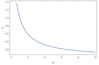
Figure 2: Quantum capacity ${\cal Q}$ (37) of a generic cosmological expansion in terms of the particles produced by it $N_{i}$ for a single-mode input $i$.

The constrained classical capacity, $C(E)$, assumes the value $h\left(\frac{1}{2}+E\right)$ when $N_{i}=0$ and decreases to $\log(1+E)$ as $N_{i}\to\infty$. The behaviour of the constrained classical capacity is shown in Fig. 1 for $E=10$, encoding particles. Instead, the quantum capacity is infinite when $N_{i}=0$ - with no surprise, since in that case we have the identity channel and infinite encoding particles - and drops to zero by increasing the number of particles, as shown in Fig. 2.

Concluding, the scenario involving less particle production is the scenario preserving more classical and quantum information from one-mode bosonic Gaussian states from the remote past.

Now, as an interesting comparison, it is worth comparing this result with the case developed in Ref. [31], where qubit states are communicated instead of Bosonic states. There, a cosmological expansion acting on a qubit leads to a transmissivity $\tau<1$, i.e., an amplitude damping channel. This is due to the different statistics involving bosonic systems and qubit systems. Indeed, reminding that a qubit comes with the occupation numbers in a fermion field momentum mode, the Pauli principle prevents an amplification of the amplitude. Nevertheless, the damping of a qubit with momentum $k$ - and, so, the loss of its classical and quantum information - is proportional to the amount of particles produced in the mode $k$ by the cosmological expansion. Then, in analogy to the bosonic case, also qubit systems’ information is better preserved as cosmological particle production is minimized. For the bosonic case, the loss of information is due to an amplification of the input, whereas for the qubit case, it is due to an amplitude damping.

IV Preserving information in $f(Q)$ non-metric gravity cosmology

With the above requirements, we wonder whether modified gravity can increase or decrease the preservation of information.

Particularly, as shown in Ref. [74], the rate of particles produced by a cosmological expansion changes by extending the Hilbert-Einstein action through additional geometric terms.

So, we here focus on STEGR, where curvature is replaced by non-metric term [50, 55].

Differently from GR, in STEGR, the background is flat and torsionless, and gravitational effects are due to non-metricity. In GR, one uses a connection implying a covariant derivative $\nabla_{\alpha}$ such that $\nabla_{\alpha}g_{\mu\nu}=0$, i.e. the Levi-Civita connection, while in STEGR, a non-metric connection is considered, say

$$\nabla_{\alpha}g_{\mu\nu}=Q_{\alpha\mu\nu}\,,$$ (38)

where $Q_{\alpha\mu\nu}$ is the non-metricity tensor. To have STEGR equivalent to GR, the following relation is considered [54, 75]

$$R=-Q-\mathcal{D}_{\alpha}(Q^{\alpha}-\tilde{Q}^{\alpha})\,,$$ (39)

where $\mathcal{D_{\alpha}}$ is the covariant derivative w.r.t. the connections and $Q^{\alpha}=Q^{\alpha\lambda}_{\lambda}$, $\tilde{Q}^{\alpha}=Q_{\lambda}^{\lambda\alpha}$, having

$$Q=\frac{1}{4}Q_{\alpha\beta\gamma}Q^{\alpha\beta\gamma}-\frac{1}{2}Q_{\alpha\beta\gamma}Q^{\beta\alpha\gamma}-\frac{1}{4}Q_{\alpha}Q^{\alpha}+\frac{1}{2}Q_{\alpha}\tilde{Q}^{\alpha}\,,$$ (40)

providing the Hilbert-Einstein action to be

$$S_{STEGR}=-\frac{1}{2}\int\sqrt{-g}Qd^{4}x\,.$$ (41)

IV.1 Coupling with non-metricity

Following the same recipe developed to arrive to Eq. (29), with the aim of investigating cosmological particle production in STEGR, it is convenient to introduce a coupling between the scalar field and the non-metricity tensor $Q_{\alpha\mu\nu}$ defined in Eq. (38). This technique permits to understand which effects a non-minimal coupling between non-metricity and fields can provide.

To this end, we remind that the covariant derivative $\nabla_{\alpha}$ defining $Q_{\alpha\mu\nu}$ from Eq. (38) is not unique, leading to a gauge choice. Among all, we choose the so-called coincident gauge, where the connection vanishes globally and where the metricity tensor is expressed via partial derivatives [76, 77] through

$$\frac{1}{2}g^{\alpha\lambda}\left(g_{\lambda\nu,\mu}+g_{\mu\lambda,\nu}-g_{\mu\nu,\lambda}\right)=\frac{1}{2}g^{\alpha\lambda}\left(Q_{\mu\alpha\nu}+Q_{\nu\alpha\mu}-Q_{\alpha\mu\nu}\right)\,.$$ (42)

In this case, the non-metricity scalar, $Q$, reads [52, 60, 61]

$$Q=-g^{\mu\nu}\left(\left\{{}_{\beta\mu}^{\alpha}\right\}\left\{{}_{\nu\alpha}^{\beta}\right\}-\left\{{}^{\alpha}_{\beta\alpha}\right\}\left\{{}^{\beta}_{\mu\nu}\right\}\right)\,.$$ (43)

This choice is particularly convenient when studying cosmological expansions. Indeed, considering Eq. (27) and using Eq. (43), one infers

$$Q=6\left(\frac{\dot{a}}{a}\right)^{2}=6H^{2}\,,$$ (44)

where $H$ is the cosmological Hubble parameter.

Hence, similarly to Eq. (29), we can assume the following interaction

$$\mathcal{L}=\frac{1}{2}\left(g^{\mu\nu}\partial_{\mu}\Phi\partial_{\nu}\Phi+m^{2}\Phi^{2}+\zeta Q\Phi^{2}\right)\,,$$ (45)

where $\zeta$ is a dimensionless coupling constant, indicating the strength of the Yukawa-like interaction between $Q$ and $\Phi$. The modified Klein-Gordon equation reads

$$(\Box-m^{2})\Phi-\zeta Q\Phi=0\,.$$ (46)

Expanding the field into normal modes, as in Eq. (1), one gets

$$\Box\phi_{\mathbf{k}}-m^{2}\phi_{\mathbf{k}}-\zeta Q\phi_{\mathbf{k}}=0\,,$$ (47)

that can be recast using the conformal time, $\eta$, defined in Eq. (28). Precisely, the Hubble parameter is ${\displaystyle H=\frac{a^{\prime}}{a^{2}}}$ and

$$H^{\prime}=\frac{a^{\prime\prime}}{a^{2}}-2\frac{a^{\prime 2}}{a^{3}}\,,$$ (48)

so, the d’Alemebert operator $\Box$, defined with the covariant derivatives of the Levi-Civita connection w.r.t. the metric (28), becomes

$$\Box=-\frac{1}{a^{4}}\left(2a^{\prime}a\partial_{\eta}+a^{2}\partial^{2}_{\eta}\right)+\nabla^{2}\,.$$ (49)

The wavefunction $\phi_{\mathbf{k}}(\mathbf{x},\eta)$ can be rewritten in the following way

$$\phi_{\mathbf{k}}(\mathbf{x},\eta)=\frac{e^{i\mathbf{k}\cdot\mathbf{x}}}{a(\eta)\sqrt{(2\pi)^{3}}}\chi_{k}(\eta)\,.$$ (50)

Recalling,

$$\left(\frac{\chi_{k}}{a}\right)^{\prime}=\frac{\chi_{k}^{\prime}a-a^{\prime}\chi_{k}}{a^{2}}\,,$$ (51a)

$$\left(\frac{\chi_{k}}{a}\right)^{\prime\prime}=\frac{a^{3}\chi_{k}^{\prime\prime}-a^{2}a^{\prime\prime}\chi_{k}-2a^{2}a^{\prime}\chi^{\prime}_{k}+2aa^{\prime 2}\chi_{k}}{a^{4}}\,,$$ (51b)

from Eq.  (47), we obtain

$$\chi^{\prime\prime}_{k}+k^{2}\chi_{k}+a^{2}\left(m^{2}-\frac{a^{\prime\prime}}{a^{3}}+6\zeta\frac{a^{\prime 2}}{a^{4}}\right)\chi_{k}=0\,.$$ (52)

Then, by means of Eq. (48), we can write

$$\frac{a^{\prime\prime}}{a^{3}}=\frac{H^{\prime}}{a}+2H^{2}\,,$$ (53)

so that Eq. (52) becomes

$$\chi^{\prime\prime}_{k}+k^{2}\chi_{k}+a^{2}\left(m^{2}+2(3\zeta-1)H^{2}-\frac{H^{\prime}}{a}\right)=0\,.$$ (54)

Eq. (54) can be rewritten using $\omega_{in}^{2}=k^{2}+a_{in}^{2}m^{2}$, with $a_{in}\coloneqq a(\eta\to-\infty)$, namely

$$\chi^{\prime\prime}_{k}(\eta)+\omega_{in}^{2}\chi_{k}(\eta)+U(\eta)\chi_{k}(\eta)=0\,,$$ (55)

where

$$U(\eta)\equiv m^{2}(a^{2}(\eta)-a_{in}^{2})+a^{2}\left(2(3\zeta-1)H^{2}(\eta)-\frac{H^{\prime}(\eta)}{a(\eta)}\right)\,.$$ (56)

IV.2 Perturbative particle production

It is clear that Eq. (55) cannot be solved analytically. Consequently, we here present a possible strategy to perturbatively compute it, following Refs. [78, 19, 36]. Despite this method was applied as $\Phi$ couples with the scalar curvature, $R$, the subsequent generalization where $Q$ replaces $R$ appears straightforward, in the coincident gauge.

Hence, for $\eta\to-\infty$ the Minkowski spacetime is reached, so that $\chi_{k}(\eta)\to\frac{e^{-i\omega_{in}\eta}}{\sqrt{2\omega_{in}}}$ and, using this recipe as a boundary condition, Eq.  (55) can be rewritten as

$$\chi_{k}(\eta)=\frac{e^{-i\omega_{in}\eta}}{\sqrt{2\omega_{in}}}-\int_{-\infty}^{\eta}U(\eta_{1})\frac{\sin(\omega_{in}(\eta-\eta_{1}))}{\omega_{in}}\chi_{k}(\eta_{1})d\eta_{1}\,.$$ (57)

This relation can be solved by iteratively substituting $\chi_{k}(\eta_{1})$ inside the right hand side of Eq. (57).

From now on, we assume that $|U(\eta)|\ll\omega_{in}^{2}$ for each $\eta$. We will verify this assumption a posteriori in the text. In such a way, we can neglect terms involving a product of many $U(\eta)/\omega_{in}^{2}$, having a perturbative solution for $\chi_{k}(\eta)$. Hence, the zeroth, first and second order read

$$\chi_{k}^{(0)}(\eta)=\frac{e^{-i\omega_{in}\eta}}{\sqrt{2\omega_{in}}}\,,$$ (58a)

$$\chi_{k}^{(1)}(\eta)=\frac{i}{(2\omega_{in})^{3/2}}\int_{-\infty}^{\eta}\left(e^{i\omega_{in}(\eta-2\eta_{1})}-e^{-i\omega_{in}\eta}\right)U(\eta_{1})d\eta_{1}\,,$$ (58b)

$$\chi_{k}^{(2)}(\eta)=-\frac{1}{\sqrt{2\omega_{in}^{5}}}\int_{-\infty}^{\eta}d\eta_{1}\sin(\eta-\eta_{1})U(\eta_{1})\times$$ (58c)

$$\int_{-\infty}^{\eta_{1}}d\eta_{2}\sin(\eta_{1}-\eta_{2})U(\eta_{2})e^{-i\omega_{in}\eta_{2}}\,.$$

Up to the second order, the far future solution for $\chi_{k}(\eta)$ is then,

$$\chi_{k}(\eta\to+\infty)=e^{-i\omega_{in}\eta}+\chi_{k}^{(1)}(\eta\to+\infty)+\chi_{k}^{(2)}(\eta\to+\infty)\,.$$ (59)

The output modes are thus obtained by inserting Eq. (59) into Eq. (50), obtaining

$$\phi_{\mathbf{k}}^{out}(\mathbf{x},\eta)=\frac{e^{i\mathbf{k}\cdot\mathbf{x}}}{a_{f}\sqrt{(2\pi)^{3}}} \left(e^{-i\omega_{in}\eta}+\chi_{k}^{(1)}(\eta\to+\infty)\right.$$

$$\left.+\chi_{k}^{(2)}(\eta\to+\infty)\right)\,,$$ (60)

where $a_{f}\coloneqq a(\eta\to\infty)$, whereas the input modes are

$$\phi_{\mathbf{k}}^{in}(\mathbf{x},\eta)=\frac{e^{i\mathbf{k}\cdot\mathbf{x}}}{a_{in}\sqrt{(2\pi)^{3}}}\,.$$ (61)

Using now Eq. (3), the Bogoliubov coefficients, Eqs. (32a) - (32b), can be found as

$$\alpha_{k}=\frac{a_{f}}{a_{in}}\left(1+\frac{i}{2\omega_{in}}\int_{-\infty}^{+\infty}d\eta_{1}U(\eta_{1})+\frac{1}{4\omega_{in}^{2}}\int_{-\infty}^{+\infty}\int_{-\infty}^{+\infty}d\eta_{1}d\eta_{2}U(\eta_{1})U(\eta_{2})(e^{2\omega_{in}i(\eta_{1}-\eta_{2})}-1)\right)\,,$$ (62a)

$$\beta_{k}=-\frac{a_{f}}{a_{in}}\left(\frac{i}{2\omega_{in}}\int_{-\infty}^{+\infty}d\eta_{1}e^{-2i\omega_{in}\eta_{1}}U(\eta_{1})+\frac{1}{4\omega_{in}^{2}}\int_{-\infty}^{+\infty}\int_{-\infty}^{+\infty}d\eta_{1}d\eta_{2}e^{2\omega_{in}i(\eta_{2}-\eta_{1})}U(\eta_{1})U(\eta_{2})\right)\,.$$ (62b)

The number of produced particles then reads

$$N_{k}=|\beta_{k}|^{2}=\frac{a_{f}^{2}}{4a_{in}^{2}\omega_{in}^{2}}\left|\int_{-\infty}^{+\infty}d\eta_{1}e^{-2i\omega_{in}\eta_{1}}U(\eta_{1})\right|^{2}\,.$$ (63)

IV.3 Affecting particle production through $f(Q)$

The STEGR extensions involve analytical functions of $Q$, say $f(Q)$, in lieu of $Q$, modifying the action, Eq. (41), as [51, 52]

$$S_{f(Q)}=-\frac{1}{2}\int\sqrt{-g}f(Q)d^{4}x\,.$$ (64)

In this case, the Friedmann equations are [54, 60, 62]

$$H^{2}=\frac{\rho+\frac{1}{2}f(Q)}{6f_{Q}}\,,$$ (65a)

$$\frac{H^{\prime}}{a}=-\frac{1}{2}\frac{\rho+p}{12H^{2}f_{QQ}+f_{Q}}\,,$$ (65b)

where $\rho$ and $p$ are the density and pressure, respectively. Clearly, we can recover the standard Friedmann equations in GR, as $f(Q)\rightarrow Q=6H^{2}$.

From Eq. (65), the inclusion of a further $f(Q)$ fluid implies a different evolution of the Hubble parameter, $H(\eta)$, and, then, from Eqs.  (63) and (56), an expected different particle production. Namely, fixing the parameters $\rho$ and $p$, Eq. (65) gives the new solution for the Hubble parameter in terms of $\eta$. Since $H(\eta)$ changes, also the scale factor $a(\eta)$ changes depending on the $f(Q)$ theory chosen, becoming

$$a_{mod}(\eta)=\left(\frac{1}{a_{in}}-\frac{1}{\sqrt{6}}\int_{-\infty}^{\eta}\sqrt{\frac{\rho(\eta^{\prime})+\frac{1}{2}f(Q)}{f_{Q}}}d\eta^{\prime}\right)^{-1}\,.$$ (66)

In turn, the function $U(\eta)$ from Eq. (56) becomes

$$U(\eta)\coloneqq m^{2}(a_{mod}^{2}(\eta)-a_{in}^{2})+a^{2}_{mod}(\eta)\left((3\zeta-1)\frac{\rho+\frac{1}{2}f(Q)}{3f_{Q}}+\frac{f_{Q}}{2}\frac{\rho+p}{2\rho f_{QQ}+f(Q)f_{QQ}+f_{Q}^{2}}\right)\,.$$ (67)

The particle production in a modified gravity theory $f(Q)$ can be computed plugging $U(\eta)$ from Eq. (67) into Eq. (63). Moreover, in Eq. (63), $a_{f}$ is now given by $a_{mod}(\eta\to+\infty)$.

Among the modified gravity theories $f(Q)$, only a part of them involves a finite particle production from remote past to future infinity. Indeed, from Eq. (63), to have a finite result for $N_{k}$, we need $a_{mod}$, from Eq. (66), to be asymptotically constant for $\eta\to 0$. This implies that $H^{2}$ drops to zero at infinite future and, so, since $Q=6H^{2}$, we need $f(Q)$ well-behaves as $Q\to 0$.

Moreover, from local observations of the gravitational constant, recalling that in $f(Q)$ theories, we have [54, 65]

$$8\pi G_{eff}\equiv\frac{1}{f_{Q}(Q)}\,.$$ (68)

To require consistency in the Solar System, we need $8\pi G_{eff}$ not to deviate from unity, at far future, i.e. for $Q\to 0$.

Then, to allow $f(Q)$ theories to have a finite particle production, we need to select suitable models. For example, we may consider a power-law approach, [52, 64, 61],

$$f(Q)=Q+\epsilon A\left(\frac{Q}{A}\right)^{d}\,,$$ (69)

where $A>0$. The above scenario reduces to the standard $\Lambda$CDM model for $d=0$ and appears quite consistent with the constraints imposed from Big Bang Nucleosynthesis [79, 80, 81]. In the far future, $f(Q)$ is finite if $d\geq 0$ and for $8\pi G_{eff}$ we have

$$8\pi G_{eff}=\begin{cases}&\frac{1}{1+\epsilon}\quad\text{if}\quad d=1\,;\\ &1\quad\text{if}\quad d=0\quad\text{or}\quad d>1\,;\\ &0\quad\text{otherwise}\,.\end{cases}$$ (70)

Then, the parameters in Eq. (69) can be either $d=0$ or $d\geq 1$, where the equality holds as long as $\epsilon\ll 1$.

V Particle production in asymptotically flat spacetimes

Besides the choices of $f(Q)$, particle production requires spacetimes to be flat at asymptotic regimes. In Einstein-de Sitter universes, this cannot be easily accounted, i.e., as the universe is dominated by precise fluids, there is no chance to guarantee the flatness. To this end, we may now consider a very precise example of cosmological expansion in which particle production easily occurs.

The model has been firstly presented in Ref. [71] through the proposed scale factor,

$$a(\eta)=\frac{1}{\sqrt{2}}\sqrt{\left(1+a_{in}^{2}+(1-a_{in}^{2})\tanh(r\eta)\right)}\,.$$ (71)

and refers to as Bernard-Duncan model, with $r$ measuring the expansion rate. The great advantage of such an approach is that $a(\eta)$ becomes constant for $\eta\to\pm\infty$, fulfilling the requirements needed to use the prescription reported in Sec. III.

The study of the particle production is performed by considering $3$ different couplings $\zeta$ between the scalar field and the non-metricity scalar $Q$ (see the Lagrangian density in Eq. (45)), i.e. $\zeta=0$ (minimal coupling), $\zeta=1/3$ (nullifying the term $\propto H^{2}$ in the right-hand side of Eq. (56)) and $\zeta=2/3$. In this way, considering Eq. (71), the condition $|U(\eta)|\ll\omega_{in}^{2}$ validating the perturbative approach in Sec. IV.2, is satisfied if $1-a_{in}^{2}\ll\omega_{in}^{2}/m^{2}$ and $r^{2}\ll\omega_{in}^{2}$.

To satisfy the first condition, we may consider the production of massless particles. Bearing this request in mind, perturbative condition turns out to be immediately fulfilled. So, having $m=0$, since $k=\omega_{in}=\omega$, the particle production, in Eq. (63), becomes $N_{\omega}$, conventionally fixing $\omega=0.1$ and $r=0.01$.

Accordingly, we can find $p(\eta)$ and $\rho(\eta)$ by putting Eq. (71) into Eq. (65) when $f(Q)=Q$ and, then, from Eq. (67), we get $\max_{\eta}|U(\eta)|<5\cdot 10^{-5}$, so that $|U(\eta)|\ll\omega^{2}$ is satisfied.

$\zeta$	$N_{\omega=0.1}$	$C(E=10)$	$\mathcal{Q}$
$0$	$1.5831\cdot 10^{-25}$	$4.8345$	$82.3854$
$1/3$	$1.5833\cdot 10^{-25}$	$4.8345$	$82.3853$
$2/3$	$4.7439\cdot 10^{-25}$	$4.8345$	$80.8021$

Table 1: In this table, the production of massless particles $N_{\omega=0.1}$ (Eq. (63)), the constrained classical capacity $C(E=10)$ (Eq. (36)) and the quantum capacity $\mathcal{Q}$ (Eq. (37)) are reported for a Bernand-Duncan cosmological expansion (71), with $r=0.01$ and $a_{in}=0.5$, for different values of the coupling $\zeta$ between the scalar field and the non-metricity scalar $Q$. The small cosmological particle production $N_{\omega=0.1}$ has practically no influence on the amount of classical information $C(E=10)$ a one-mode Gaussian state could preserve. On the contrary, the maximum amount of quantum information reliably stored by a Gaussian state $\mathcal{Q}$ is affected by the cosmological particle production $N_{\omega=0.1}$ even if very small.

In so doing, we can calculate the particle production numerically from Eq. (63) and the classical and quantum capacity by putting $N_{k}=N_{\omega}$ in Eqs. (36) and (37), respectively.

The corresponding numerical outcomes have been reported in table 1.

Switching to the classical capacity, if $N_{\omega}\ll 1$ and $E\gg N_{\omega}$, from Eq. (36), we immediately have

$$C(E)\sim h\left(\frac{1}{2}+E\right)+N_{\omega}\log N_{\omega}\,.$$ (72)

As a consequence, as long as the particle production is very low, the classical capacity is practically unaffected by it, as shown in the table 1.

The situation appears quite different for the quantum capacity. Indeed, from Tab. 1, we see that $\mathcal{Q}$ slightly changes, for different $N_{\omega}$, even if $N_{\omega}\ll 1$.

V.1 Power-law modification of non-metric gravity

We now see how the particle production and the capacities reported in Tab. 1 change by considering a modified gravity theory $f(Q)$. Namely, we consider the power-law gravity modification in Eq. (69), where we conventionally fix the parameter $A$ as $A\sim Q$, and, in particular, we select $A=\max_{\eta}\{2\rho(\eta)\}\sim 1.418\cdot 10^{-4}$.

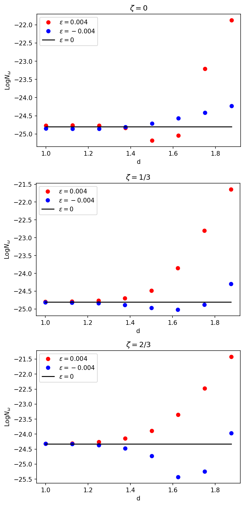
Figure 3: Number of massless scalar particles $N_{\omega}$, with frequency $\omega=0.1$, produced under a cosmological expansion given by the scale factor (71) (with $a_{in}=0.5$ and $r=0.01$) vs the parameter $d$ of the modified gravity theory $f(Q)$ from Eq. (69), where $A\simeq 1.418\cdot 10^{-4}$. The particle production $N_{\omega}$ is shown for different values of the coupling $\zeta$ between the particles’ field and the non-metricity scalar $Q=6H^{2}$, and for different values of $\epsilon$, another parameter of the modification $f(Q)$ from Eq. (69).

With these parameters, the particle production was computed numerically inserting Eq. (67) into Eq. (63). The results are shown in Fig. 3 for different values of $\zeta$, $d$ and $\epsilon$ (the unmodified case, from Eq. (69) corresponds to $\epsilon=0$).

As expected, the behaviour of the particle production is different depending on the sign of $\epsilon$. In case $\zeta=1/3$ or $\zeta=2/3$ the particle production $N_{\omega}$ is lower than the one obtained in general relativity only if $\epsilon<0$ and when $d$ assumes values in a bounded interval. Otherwise, if $\epsilon>0$, the particle production $N_{\omega}$ always increases with respect to the unmodified case $\epsilon=0$.

An opposite tendency can be observed from Fig. 3 in the minimal coupling case $\zeta=0$, where the particle production $N_{\omega}$ is minimized when $\epsilon>0$. If $\epsilon<0$, we still have a decreasing of the particle production w.r.t. the unmodified case, but this is much smaller than the one get when $\epsilon>0$.

Since we showed in table 1 that classical capacity is unaffected by a very low production of particles (see Table 1), we now focus on the quantum capacity only. Then, we analyze how much the quantum capacities, reported in Tab. 1, depart from GR, through extending it by virtue of $f(Q)$, see Fig. 3. For each coupling $\zeta$ the highest quantum capacity occurs when $d=d_{min}$, minimizing the particle production to $\underline{N}_{\omega}$. Then, we can quantify the maximum gain of quantum capacity through

$$\Delta\mathcal{Q}=\frac{\mathcal{Q}(N_{\omega}=\underline{N}_{\omega})-\mathcal{Q}(\epsilon=0)}{\mathcal{Q}(\epsilon=0)}\,.$$ (73)

The values of $\Delta\mathcal{Q}$ are reported in Tab. 2, as well as the numerically computed values of $d_{min}$.

$\zeta$	$\epsilon$	$d_{min}$	$\Delta\mathcal{Q}$
$0$	$0.004$	$1.59$	$4.23\%$
$1/3$	$-0.004$	$1.61$	$0.89\%$
$2/3$	$-0.004$	$1.69$	$7.76\%$

Table 2: In this table we report, for each value of the coupling $\zeta$, the maximum gain of quantum capacity $\Delta\mathcal{Q}$ (from Eq. (73)) achievable with the modified gravity theory (69) by bounding $|\epsilon|=0.004$. In the second and third columns we report respectively the values of the parameters $\epsilon$ and $d$ of the power law modification needed to reach the gain $\Delta\mathcal{Q}$.

In general, we proved that, for each coupling $\zeta$, there is a polynomial $f(Q)$ model, with parameters established in table 2, preserving quantum information from remote past better than general relativity. With these theories, we are able to reach a modest increasing on the conserved quantum information (up to $4.23\%$ in case of minimal coupling $\zeta=0$). Moreover, these modified theories also preserve the GR gravitational coupling in the far future, so that local observations would not be disrupted by them.

VI Discussion and Conclusions

In this work, we investigated the maximum amount of classical and quantum information that a one-mode Gaussian state can reliably preserve from the remote past through cosmological expansion. To achieve this, we developed a general method based on quantum communication theory, recognizing the Bogoliubov transformations of one-mode bosonic states as quantum channels. We analyzed their properties and capacities in terms of the Bogoliubov coefficients, i.e., adopting a method also useful for studying how entanglement entropy evolves from the remote past to the distant future, as reported in Appendices A and B.

Particularly, for a generic cosmological expansion in a homogeneous and isotropic universe, the resulting particle production is shown to be responsible for amplifying bosonic signals that originate from the remote past. Consequently, the classical and quantum information, encoded in these signals, degrades due to the cosmological particle production. We focused on the cosmological scenario that best preserves information from the remote past, finding that it represents the one with the least amount of produced particles.

As reported in detail in Appendix B, we demonstrated that entanglement, originating from the remote past, is most significantly enhanced by increasing cosmological particle production. We showed that this result extends the well-known phenomenon of entanglement creation from vacuum by a cosmological expansion for each initial maximally entangled state. In this context, it is shown that entanglement from the remote past always increases when the initial number of entangled particles is small. However, if the initial entanglement entropy is sufficiently high, this enhancement is not always guaranteed. Indeed, for certain values of the phase of the Bogoliubov coefficients, cosmological particle production may even lead to entanglement degradation.

In this respect, we also investigated how modified theories of gravity that lead to different results. We thus focused on $f(Q)$ theories of gravity, in which analytical functions of non-metricity are involved. Precisely, we circumscribed our analysis to those theories that can decrease particle production. To this end, we showed that very simple power-law modifications, with appropriate set of free parameters matching local observation, can optimize the preservation of classical and quantum information stored in bosons from remote past. Notably, while classical information preserved in a system remains unaffected by small particle production, the quantum information in the same system can be significantly compromised even with minimal cosmological particle production.

By adjusting the parameters of the power-law gravity modification, the amount of preserved quantum information can increase up to $4.23\%$ compared to the prediction of GR, in the case of minimal coupling ($\zeta=0$). By increasing the coupling to $\zeta=2/3$, $f(Q)$ theories can increase the maximum amount of conserved quantum information, up to $\sim 8\%$.

Summing up, the results here obtained may therefore open the possibility of detecting cosmological particle production through the study of the degradation of qubit information content. Consequently, the ability to achieve cosmological particle production, including through analog gravity systems [82], offers a pathway to distinguish between modified theories of gravity and the coupling between fields and curvature (or non-metricity). In conclusion, cosmological particle production serves as a crucial tool for understanding the evolutionary history of our universe, particularly during the inflationary epoch, which is believed to have generated a substantial quantity of particles [83, 84, 85]. Recent studies have explored models linking dark matter to this particle production process [86, 87, 88]. Within this framework, the reduction in communication capacities due to particle production holds profound implications. It is plausible that the dark particles produced during inflation could obscure information regarding particles from the remote past. As a result, this research, along with related studies focusing on fermions [31], may establish fundamental limits on our ability to recover information about primordial particles.

Appendix A Entropy and entanglement of bosonic Gaussian states

Here we provide further mathematical information on the BGSs studied in Sec. II, focusing on their Von Neumann entropy and on their entanglement entropy. A two-modes Gaussian state (modes $i,j$) can be written, from Eqs. (4), (8) and (9), as

$$\sigma=\left(\begin{matrix}\frac{1}{2}+n_{i}+\real m_{i}&\imaginary m_{i}&\real\gamma_{ij}+\real\chi_{ij}&\imaginary\gamma_{ij}+\imaginary\chi_{ij}\\ \imaginary m_{i}&\frac{1}{2}+n_{i}-\real m_{i}&-\imaginary\gamma_{ij}+\imaginary\chi_{ij}&\real\gamma_{ij}-\real\chi_{ij}\\ \real\gamma_{ij}+\real\chi_{ij}&-\imaginary\gamma_{ij}+\imaginary\chi_{ij}&\frac{1}{2}+n_{j}+\real m_{j}&\imaginary m_{j}\\ \imaginary\gamma_{ij}+\imaginary\chi_{ij}&\real\gamma_{ij}-\real\chi_{ij}&\imaginary m_{j}&\frac{1}{2}+n_{j}-\real m_{j}\end{matrix}\right)\,,$$ (74)

where $\gamma_{ij}=\langle a_{i}^{\dagger}a_{j}\rangle$, $\chi_{ij}=\langle a_{i}a_{j}\rangle$. The calculation of the symplectic eigenvalues of $4\times 4$ definite positive matrices is provided in literature (see e.g. Ref. [89]) and they are

$$\nu_{\pm}=\frac{1}{\sqrt{2}}\sqrt{\Gamma\pm\sqrt{\Gamma^{2}-4\det\sigma}}\,,$$ (75)

where we defined the parameter $\Gamma\coloneqq\nu_{i}^{2}+\nu_{j}^{2}+2\left(|\gamma_{ij}|^{2}-|\chi_{ij}|^{2}\right)$ with $\nu_{i}$ ($\nu_{j}$) the symplectic eigenvalue of the covariance matrix of the subsystem state $\sigma_{ii}$ ($\sigma_{jj}$), given by

$$\nu_{i}\coloneqq\sqrt{\det\sigma_{ii}}$$ (76)

The Von Neumann entropy of the two mode Gaussian state is then

$$\mathcal{S}(\sigma)=h(\nu_{-})+h(\nu_{+})\,.$$ (77)

A maximally entangled state is a composite pure state with zero entropy and where the entropy of one of its subsystem states - also called entanglement entropy $\mathcal{S}_{E}$ - is maximized. Fixing the average number of particles in each subsystem state $n_{i}=n_{j}$, a maximally entangled two-modes Gaussian state is provided when $m_{i}=0$, $\gamma_{ij}=0$ and $|\chi_{ij}|=\sqrt{n_{i}(n_{i}+1)}$. The covariance matrix of this state is

$$\sigma=\left(\begin{matrix}\frac{1}{2}+n_{i}&0&\sqrt{n_{i}(n_{i}+1)}\cos\theta&\sqrt{n_{i}(n_{i}+1)}\sin\theta\\ 0&\frac{1}{2}+n_{i}&\sqrt{n_{i}(n_{i}+1)}\sin\theta&-\sqrt{n_{i}(n_{i}+1)}\cos\theta\\ \sqrt{n_{i}(n_{i}+1)}\cos\theta&\sqrt{n_{i}(n_{i}+1)}\sin\theta&\frac{1}{2}+n_{i}&0\\ \sqrt{n_{i}(n_{i}+1)}\sin\theta&-\sqrt{n_{i}(n_{i}+1)}\cos\theta&0&\frac{1}{2}+n_{i}\end{matrix}\right)\,,$$ (78)

where $\theta$ is the phase of $\chi_{ij}$. Its entanglement entropy is

$$\mathcal{S}_{E}(\sigma)=h\left(\frac{1}{2}+n_{i}\right)\,,$$ (79)

and it is proportional on the average number of entangled particles $n_{i}$.

Appendix B Entanglement preservation after a cosmological expansion

From the literature (see e.g. [37, 38, 39]), it is well known that the particles created from vacuum, with momentum $\mathbf{k}$ by a cosmological expansion are maximally entangled with the particle created from vacuum with momentum $-\mathbf{k}$. By virtue of this, one may think that particle production reinforces any pre-existing entanglement. We show in this appendix that this is not the case. Namely, there can be states whose entanglement is degraded by particle production.

From now on, calling $i$ the mode relative to the momentum $\mathbf{k}$, we refer with $-i$ to the mode relative to its opposite momentum $-\mathbf{k}$. We then simplify Eqs. (15), (16), (17) and (18) using the Bogoliubov coefficients (32a) and (32b), getting

$$\tilde{n}_{i}=|\alpha_{i}|^{2}n_{i}+|\beta_{i}|^{2}(1+n_{-i})-2\real\left(\alpha_{i}^{\ast}\beta_{i}\chi_{i,-i}\right)\,;$$ (80)

$$\tilde{m}_{i}=\alpha_{i}^{\ast 2}m_{i}+\beta_{i}^{\ast 2}m_{-i}-2\alpha_{i}\beta_{i}^{\ast}\gamma_{i,-i}^{\ast}\,.$$ (81)

$$\tilde{\gamma}_{i,-i}=-\alpha_{i}\beta_{i}^{\ast}m_{i}^{\ast}-\alpha_{i}^{\ast}\beta_{i}m_{-i}+(|\alpha_{i}|^{2}+|\beta_{i}|^{2})\gamma_{i,-i}\,;$$ (82)

$$\tilde{\chi}_{i,-i}=-\alpha_{i}^{\ast}\beta_{i}^{\ast}(1+n_{i})-\beta_{i}^{\ast}\alpha_{i}^{\ast}n_{-i}+(\alpha_{i}^{\ast 2}+\beta_{i}^{\ast 2})\chi_{i,-i}\,.$$ (83)

As specified in Eq. (78), a maximally entangled two-modes Gaussian state with number of particles in the subsystem states $n_{i}=n_{-i}$ is characterized by the covariance matrix (74) with $m_{\pm i}=0$, $\gamma_{i,-i}=0$ and $\chi_{i,-i}=\sqrt{n_{i}(n_{i}+1)}e^{i\theta}$ for an arbitrary $\theta$. The state after the cosmological expansion, called $\tilde{\sigma}$, is again characterized by the two-modes state (74) with $\tilde{n}_{\pm i}$, $\tilde{m}_{\pm i}$, $\tilde{\gamma}_{i,-i}$ and $\tilde{\chi}_{i,-i}$ replacing $n_{\pm i}$, $m_{\pm i}$, $\gamma_{i,-i}$ and $\chi_{i,-i}$, respectively. Using Eqs. (80), (81), (82) and (83), we get

$$\tilde{n}_{\pm i}=(1+2N_{i})n_{i}+N_{i}-2\real(\alpha^{\ast}_{i}\beta_{i}\chi_{i,-i})\,;$$ (84)

$$\tilde{m}_{i}=0\,;$$ (85)

$$\tilde{\gamma}_{\pm i,\mp i}=0\,;$$ (86)

$$\tilde{\chi}_{\pm i,\mp i}=-\alpha_{i}^{\ast}\beta_{i}^{\ast}(1+2n_{i})+\alpha_{i}^{\ast 2}\chi_{i,-i}+\beta_{i}^{\ast 2}\chi_{i,-i}^{\ast}\,.$$ (87)

If we study the symplectic eigenvalues of the state (75) using the parameters (84), (85), (86) and (87) we get that they are both $1/2$. As a consequence, from Eq. (77), the entropy of the cosmological expansion output $\tilde{\sigma}$ is zero. This means that $\tilde{\sigma}$ is still a maximally entangled state and its entanglement entropy is

$$\mathcal{S}_{E}(\tilde{\sigma}) =h\left(\frac{1}{2}+\tilde{n}_{i}\right)=h\left(\frac{1}{2}+n_{i}+N_{i}(1+2n_{i})\right.$$

$$\left.-2\sqrt{n_{i}(n_{i}+1)}\sqrt{N_{i}(N_{i}+1)}\cos(\varphi+\theta)\right)\,,$$ (88)

where we defined $\varphi$ from $\alpha_{i}^{\ast}\beta_{i}=\sqrt{N_{i}(N_{i}+1)}e^{i\varphi}$. We can immediately verify that the result is consistent with the literature [37, 38, 39] in the vacuum case, i.e. for $n_{i}=0$. To have the enhancement of entanglement, we need $\mathcal{S}_{E}(\sigma)<\mathcal{S}_{E}(\tilde{\sigma})$, occurring when $n_{i}<\tilde{n}_{i}$, i.e. when

$$\cos(\theta+\varphi)<\frac{1+2n_{i}}{2\sqrt{n_{i}(n_{i}+1)}}\sqrt{\frac{N_{i}}{N_{i}+1}}\,.$$ (89)

The condition (89) is strongly dependent on the parameter $\theta$ of the initially entangled state (78) (assuming $\varphi$ fixed by the cosmic expansion). Namely, in terms of $\theta$, the condition for the entanglement enhancement becomes

$$\theta\notin \left(\arccos\left(\frac{1+2n_{i}}{2\sqrt{n_{i}(n_{i}+1)}}\sqrt{\frac{N_{i}}{N_{i}+1}}\right)-\varphi,\right.$$

$$\left.-\arccos\left(\frac{1+2n_{i}}{2\sqrt{n_{i}(n_{i}+1)}}\sqrt{\frac{N_{i}}{N_{i}+1}}\right)-\varphi\right)\,.$$ (90)

Instead, if $\theta$ belongs to the interval specified in Eq. (90), the entanglement in the far future is less than the one at remote past. Namely, the cosmological expansion causes entanglement degradation. In this case, comparing the initial entanglement entropy with the final one, in Eq. (B), we can easily seen that the amount of entanglement degraded vanishes for $N_{i}\to 0$. Hence, the scenario with less particle production, researched throughout the paper, is the one reducing the degradation of entanglement if the condition (90) is not satisfied.

For the sake of completeness, it is worth noticing that, if the particle production is enough high, the entanglement of a state from the remote past is always enhanced by the cosmological expansion, regardless the value of $\theta$. This happens when the right hand side of Eq. (89) is greater than $1$, namely when

$$N_{i}>4n_{i}+4n_{i}^{2}.$$ (91)

This is consistent with the fact that, starting from the vacuum $n_{i}=0$, the creation of entanglement is guaranteed by the particle production. To conclude, if the aim is maximizing the entanglement at the far future, a high particle production scenario is preferable, so that Eq. (91) is satisfied. However, if the aim is to better preserve entanglement from the remote past, for each number of initially entangled particles $n_{i}$, the preferable scenario is the one minimizing the particle production.

References

- [1] C. E. Shannon. A mathematical theory of communication. The Bell System Technical Journal, 27(3):379–423, July 1948.
- [2] R. Gatenby and R. Frieden. Information theory in living systems, methods, applications, and challenges. Bulletin of mathematical biology, 69(2):635–57, March 2007.
- [3] S. Mancini and A. Winter. A Quantum Leap in Information Theory. World Scientific, 2019.
- [4] J. D. Bekenstein and M. Schiffer. Quantum limitations on the storage and transmission of information. Int. J. Mod. Phys. C, 01(04):355–422, December 1990.
- [5] J. D. Bekenstein. Information in the holographic universe. Scientific American, 289(2):58–65, August 2003.
- [6] J. S. Sidhu et Al. Advances in space quantum communications. IET Quantum Communication, 2(4):182–217, July 2021.
- [7] A. D. Dolgov and M. Kawasaki. Can modified gravity explain accelerated cosmic expansion? Phys. Lett. B, 573:1–4, October 2003.
- [8] V. Faraoni and A. Jacques. Cosmological expansion and local physics. Phys. Rev. D, 76(6):063510, September 2007.
- [9] R. B. Mann and T. C. Ralph. Relativistic quantum information. Class. Quantum Grav., 29(22):220301, November 2012.
- [10] Č. Brukner. Quantum causality. Nature Physics, 10(4):259–263, April 2014.
- [11] J. de Ramón, M. Papageorgiou, and E. Martín-Martínez. Causality and signalling in noncompact detector-field interactions. Phys. Rev. D, 108(4):045015, August 2023.
- [12] S. L. Braunstein and A. K. Pati. Quantum information cannot be completely hidden in correlations: implications for the black-hole information paradox. Phys. Rev. Lett., 98(8):080502, February 2007.
- [13] B. Chen, B. Czech, and Z. Wang. Quantum information in holographic duality. Reports on Progress in Physics, 85(4):046001, March 2022.
- [14] Salvatore Capozziello, Silvia De Bianchi, and Emmanuele Battista. Avoiding singularities in Lorentzian-Euclidean black holes: The role of atemporality. Phys. Rev. D, 109(10):104060, May 2024.
- [15] T. W. Van De Kamp, R. J. Marshman, S. Bose, and A. Mazumdar. Quantum gravity witness via entanglement of masses: Casimir screening. Phys. Rev. A, 102(6):062807, December 2020.
- [16] M. Christodoulou et Al. Locally mediated entanglement in linearized quantum gravity. Phys. Rev. Lett., 130(10):100202, March 2023.
- [17] D. E. Bruschi, N. Friis, I. Fuentes, and S. Weinfurtner. On the robustness of entanglement in analogue gravity systems. New Journal of Physics, 15(11):113016, November 2013.
- [18] M. Jacquet, S. Weinfurtner, and F. Koenig. The next generation of analogue gravity experiments. Philosophical Transactions A, 378(2177):20190239, July 2020.
- [19] N. D. Birrell and P. C. W. Davies. Quantum Fields in Curved Space. Cambridge Monographs on Mathematical Physics. Cambridge Univ. Press, Cambridge, UK, 1984.
- [20] L. Parker and D. Toms. Quantum Field Theory in Curved Spacetime: Quantized Fields and Gravity. Cambridge Monographs on Mathematical Physics. Cambridge University Press, 2009.
- [21] C. Anastopoulos, B. Hu, and K. Savvidou. Quantum field theory based quantum information: Measurements and correlations. Ann. Phys., 450:169239, March 2023.
- [22] T. R. Perche and E. Martín-Martínez. Role of quantum degrees of freedom of relativistic fields in quantum information protocols. Phys. Rev. A, 107(4):042612, April 2023.
- [23] W. G. Unruh. Notes on black-hole evaporation. Phys. Rev. D, 14(4):870–892, August 1976.
- [24] W. G. Unruh and R. M. Wald. What happens when an accelerating observer detects a rindler particle. Phys. Rev. D, 29(6):1047–1056, March 1984.
- [25] B. L. Hu, S. Lin, and J. Louko. Relativistic quantum information in detectors–field interactions. Class. Quantum Grav., 29(22):224005, October 2012.
- [26] E. G. Brown, E. Martín-Martínez, N. C. Menicucci, and R. B. Mann. Detectors for probing relativistic quantum physics beyond perturbation theory. Phys. Rev. D, 87(8):084062, April 2013.
- [27] E. Tjoa and K. Gallock-Yoshimura. Channel capacity of relativistic quantum communication with rapid interaction. Phys. Rev. D, 105(8):085011, April 2022.
- [28] A. Lapponi, D. Moustos, D. E. Bruschi, and S. Mancini. Relativistic quantum communication between harmonic oscillator detectors. Phys. Rev. D, 107(12):125010, June 2023.
- [29] A. Lapponi, J. Louko, and S. Mancini. Making two particle detectors in flat spacetime communicate quantumly. arXiv:2404.01880, April 2024. Accepted in Phys. Rev. D in June 2024.
- [30] K. Brádler and C. Adami. The capacity of black holes to transmit quantum information. J. High Energy Phys., 2014(095), May 2014.
- [31] S. Mancini, R. Pierini, and M. M. Wilde. Preserving information from the beginning to the end of time in a robertson–walker spacetime. New Journal of Physics, 16(12):123049, December 2014.
- [32] G. Gianfelici and S. Mancini. Quantum channels from reflections on moving mirrors. Scientific Reports, 7(1):15747, November 2017.
- [33] M. R. R. Good, A. Lapponi, O. Luongo, and S. Mancini. Quantum communication through a partially reflecting accelerating mirror. Phys. Rev. D, 104(10):105020, November 2021.
- [34] E. T. Jaynes and F. W. Cummings. Comparison of quantum and semiclassical radiation theories with application to the beam maser. Proceedings of the IEEE, 51(1):89–109, February 1963.
- [35] D. E. Bruschi, A. R. Lee, and I. Fuentes. Time evolution techniques for detectors in relativistic quantum information. J. Phys. A: Mathematical and Theoretical, 46(16):165303, April 2013.
- [36] L. H. Ford. Cosmological particle production: a review. Reports on Progress in Physics, 84(11):116901, October 2021.
- [37] J. L. Ball, I. Fuentes-Schuller, and F. P. Schuller. Entanglement in an expanding spacetime. Phys. Lett. A, 359(6):550–554, December 2006.
- [38] I. Fuentes, R. B. Mann, E. Martín-Martínez, and S. Moradi. Entanglement of Dirac fields in an expanding spacetime. Phys. Rev. D, 82(4):045030, August 2010.
- [39] E. Martín-Martínez and N. C. Menicucci. Cosmological quantum entanglement. Class. Quantum Grav., 29(22):224003, October 2012.
- [40] A. Serafini. Quantum Continuous Variables: A Primer of Theoretical Methods. CRC Press, 2017.
- [41] A century of correct predictions. Nature Physics, 15:415, May 2019.
- [42] S. Nojiri and S. D. Odintsov. Introduction to modified gravity and gravitational alternative for dark energy. Int. J. Geom. Methods Mod. Phys., 4(01):115–145, February 2007.
- [43] S. Capozziello and M. Francaviglia. Extended theories of gravity and their cosmological and astrophysical applications. General Relativity and Gravitation, 40(2-3):357–420, December 2007.
- [44] A. De Felice and S. Tsujikawa. theories. Living Rev. Relativ., 13(1), June 2010.
- [45] S. Capozziello and M. De Laurentis. Extended theories of gravity. Phys. Rep. , 509(4-5):167–321, December 2011.
- [46] L. Lombriser et Al. Cluster density profiles as a test of modified gravity. Phys. Rev. D, 85(10):102001, May 2012.
- [47] M. Reina-Campos, A. Sills, and G. Bichon. Initial sizes of star clusters: implications for cluster dissolution during galaxy evolution. Mon. Not. R. Astron. Soc., 524(1):968–980, September 2023.
- [48] S. Nojiri and S. D. Odintsov. Is the future universe singular: Dark matter versus modified gravity? Phys. Lett. B, 686(1):44–48, March 2010.
- [49] Z. Davari and S. Rahvar. Testing modified gravity (MOG) theory and dark matter model in Milky Way using the local observables. Mon. Not. R. Astron. Soc., 496(3):3502–3511, August 2020.
- [50] M. Adak, Ö. Sert, M. Kalay, and M. Sari. Symmetric teleparallel gravity: some exact solutions and spinor couplings. Int. J. Mod. Phys. A, 28(32):1350167, December 2013.
- [51] S. Mandal, D. Wang, and PK Sahoo. Cosmography in gravity. Phys. Rev. D, 102(12):124029, December 2020.
- [52] J. B. Jiménez, L. Heisenberg, T. Koivisto, and S. Pekar. Cosmology in geometry. Phys. Rev. D, 101(10):103507, May 2020.
- [53] Lavinia Heisenberg. Review on gravity. Phys. Rept., 1066:1–78, May 2024.
- [54] J. Jimenez, L. Heisenberg, and T. Koivisto. The geometrical trinity of gravity. Universe, 5(7):173, July 2019.
- [55] Salvatore Capozziello, Vittorio De Falco, and Carmen Ferrara. Comparing equivalent gravities: common features and differences. Eur. Phys. J. C, 82(10):865, October 2022.
- [56] S. K. Maurya, K. N. Singh, S. V. Lohakare, and B. Mishra. Anisotropic strange star model beyond standard maximum mass limit by gravitational decoupling in gravity. Fortschritte der Physik, 70(11):2200061, September 2022.
- [57] P. Bhar, S. Pradhan, A. Malik, and P. K. Sahoo. Physical characteristics and maximum allowable mass of hybrid star in the context of gravity. Eur. Phys. J. C, 83(7):646, July 2023.
- [58] Salvatore Capozziello, Maurizio Capriolo, and Shin’ichi Nojiri. Gravitational waves in non-metric gravity via geodesic deviation. Phys. Lett. B, 850:138510, March 2024.
- [59] Salvatore Capozziello and Maurizio Capriolo. Gravitational waves in non-metric gravity without gauge fixing. Phys. Dark Univ., 45:101548, June 2024.
- [60] I. S. Albuquerque and N. Frusciante. A designer approach to gravity and cosmological implications. Phys. Dark Universe, 35:100980, March 2022.
- [61] W. Khyllep, J. Dutta, E. N. Saridakis, and K. Yesmakhanova. Cosmology in gravity: A unified dynamical systems analysis of the background and perturbations. Phys. Rev. D, 107(4):044022, February 2023.
- [62] S. Capozziello and R. D’Agostino. Model-independent reconstruction of non-metric gravity. Phys. Lett. B, 832:137229, September 2022.
- [63] Shin’ichi Nojiri and S. D. Odintsov. Well-defined gravity, reconstruction of FLRW spacetime and unification of inflation with dark energy epoch. Phys. Dark Univ., 45:101538, April 2024.
- [64] I. Ayuso, R. Lazkoz, and V. Salzano. Observational constraints on cosmological solutions of theories. Phys. Rev. D, 103(6):063505, March 2021.
- [65] F. K. Anagnostopoulos, S. Basilakos, and E. N. Saridakis. First evidence that non-metricity gravity could challenge Lambda-CDM. Phys. Lett. B, 822(4):136634, November 2021.
- [66] G. Adesso, S. Ragy, and A. R. Lee. Continuous variable quantum information: Gaussian states and beyond. Open Systems & Information Dynamics, 21(01n02):1440001, March 2014.
- [67] I. Devetak and P. W. Shor. The capacity of a quantum channel for simultaneous transmission of classical and quantum information. Commun. Math. Phys. , 256:287–303, March 2003.
- [68] F. Caruso, V. Giovannetti, and A. S. Holevo. One-mode bosonic gaussian channels: a full weak-degradability classification. New Journal of Physics, 8(12):310–310, December 2006.
- [69] O. V. Pilyavets, C. Lupo, and S. Mancini. Methods for estimating capacities and rates of Gaussian quantum channels. IEEE Trans. Inf. Theory, 58(9):6126–6164, September 2012.
- [70] K. Brádler. Coherent information of one-mode Gaussian channels—the general case of non-zero added classical noise. J. Phys. A: Mathematical and Theoretical, 48(12):125301, March 2015.
- [71] C. Bernard and A. Duncan. Regularization and renormalization of quantum field theory in curved space-time. Ann. Phys., 107(1):201–221, September 1977.
- [72] L. H. Ford. Gravitational particle creation and inflation. Phys. Rev. D, 35(10):2955–2960, May 1987.
- [73] A. S. Holevo and R. F. Werner. Evaluating capacities of bosonic Gaussian channels. Phys. Rev. A, 63(3):032312, February 2001.
- [74] S. Capozziello, O. Luongo, and M. Paolella. Bounding gravity by particle production rate. Int. J. Mod. Phys. D, 25(04):1630010, March 2016.
- [75] Salvatore Capozziello, Vittorio De Falco, and Carmen Ferrara. The role of the boundary term in symmetric teleparallel gravity. Eur. Phys. J. C, 83(10):915, October 2023.
- [76] J. B. Jiménez, L. Heisenberg, and T. S. Koivisto. Teleparallel palatini theories. J. Cosmol. Astrop. P., 2018(08):039–039, August 2018.
- [77] S. Bahamonde and L. Järv. Coincident gauge for static spherical field configurations in symmetric teleparallel gravity. Eur. Phys. J. C, 82(10):963, October 2022.
- [78] Y. B. Zeldovich and A. A. Starobinsky. Particle production and vacuum polarization in an anisotropic gravitational field. Zh. Eksp. Teor. Fiz., 61:2161–2175, June 1971.
- [79] F. K. Anagnostopoulos, V. Gakis, E. N. Saridakis, and S. Basilakos. New models and big bang nucleosynthesis constraints in gravity. Eur. Phys. J. C, 83(1), January 2023.
- [80] Micol Benetti, Salvatore Capozziello, and Gaetano Lambiase. Updating constraints on teleparallel cosmology and the consistency with Big Bang Nucleosynthesis. Mon. Not. Roy. Astron. Soc., 500(2):1795–1805, June 2020.
- [81] S. Capozziello, G. Lambiase, and E. N. Saridakis. Constraining teleparallel gravity by Big Bang Nucleosynthesis. Eur. Phys. J. C, 77(9):576, August 2017.
- [82] P. Jain, S. Weinfurtner, M. Visser, and C. W. Gardiner. Analog model of a Friedmann-Robertson-Walker universe in Bose-Einstein condensates: Application of the classical field method. Phys. Rev. A, 76(3):033616, September 2007.
- [83] N. Barnaby and Z. Huang. Particle production during inflation: Observational constraints and signatures. Phys. Rev. D, 80(12), December 2009.
- [84] E. W. Kolb, S. Ling, A. J. Long, and R. A. Rosen. Cosmological gravitational particle production of massive spin-2 particles. J. High Energy Phys., 181(5), May 2023.
- [85] J. Cembranos, L. Garay, Á. Parra-López, and J. Sánchez Velázquez. Late vacuum choice and slow roll approximation in gravitational particle production during reheating. J. Cosmol. Astrop. P., 2023(08):060, August 2023.
- [86] L. Li, T. Nakama, C. M. Sou, Y. Wang, and S. Zhou. Gravitational production of superheavy dark matter and associated cosmological signatures. J. High Energy Phys., 2019(67), July 2019.
- [87] L. Li, S. Lu, Y. Wang, and S. Zhou. Cosmological signatures of superheavy dark matter. J. High Energy Phys., 2020(231), July 2020.
- [88] Z. Safari, K. Rezazadeh, and B. Malekolkalami. Structure formation in dark matter particle production cosmology. Phys. Dark Universe, 37:101092, September 2022.
- [89] J. Laurat et Al. Entanglement of two-mode gaussian states: characterization and experimental production and manipulation. J. Opt. B, 7(12):S577–S587, November 2005.