Accuracy on the wrong line: On the pitfalls of noisy data for out-of-distribution generalisation

Abstract

“Accuracy-on-the-line” is a widely observed phenomenon in machine learning, where a model’s accuracy on in-distribution (ID) and out-of-distribution (OOD) data is positively correlated across different hyperparameters and data configurations. But when does this useful relationship break down? In this work, we explore its robustness. The key observation is that noisy data and the presence of nuisance features can be sufficient to shatter the Accuracy-on-the-line phenomenon. In these cases, ID and OOD accuracy can become negatively correlated, leading to “Accuracy-on-the-wrong-line.” This phenomenon can also occur in the presence of spurious (shortcut) features, which tend to overshadow the more complex signal (core, non-spurious) features, resulting in a large nuisance feature space. Moreover, scaling to larger datasets does not mitigate this undesirable behavior and may even exacerbate it. We formally prove a lower bound on Out-of-distribution (OOD) error in a linear classification model, characterizing the conditions on the noise and nuisance features for a large OOD error. We finally demonstrate this phenomenon across both synthetic and real datasets with noisy data and nuisance features.

1 Introduction

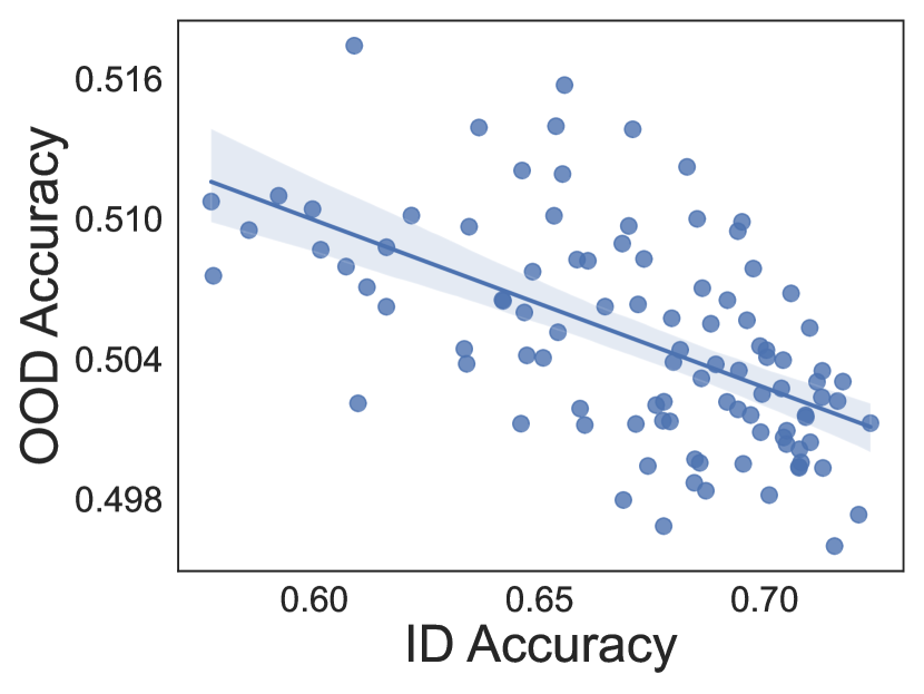
(a) Noisy dataset

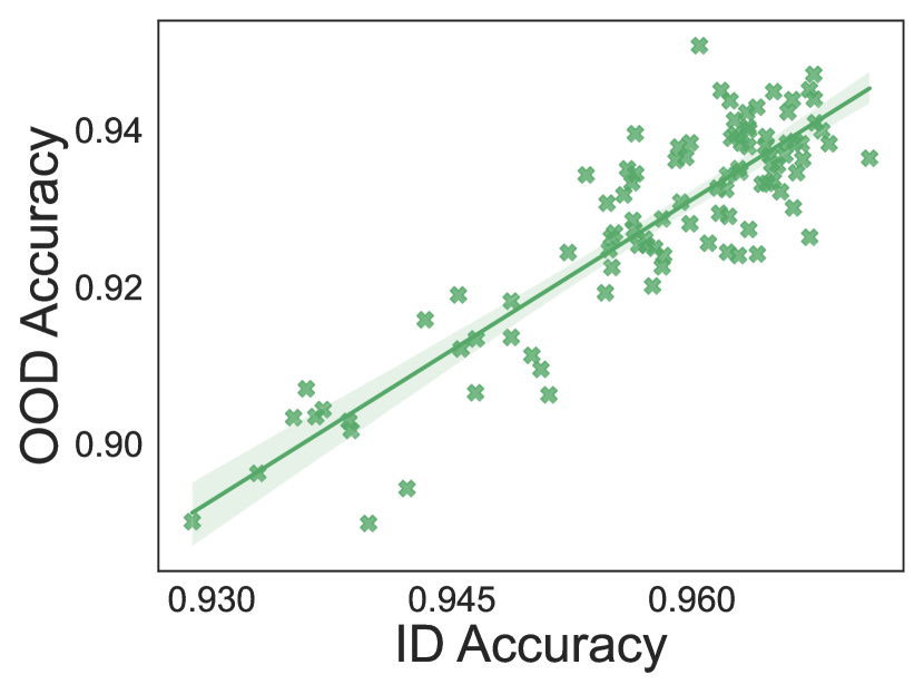
(b) Noiseless dataset

Figure 1:  Accuracy-on-the-wrong-line behaviour in Noisy dataset vs. Accuracy-on-the-line behaviour in Noiseless dataset in linear setting. See Section 4 for a description of the setting.

Machine Learning (ML) models often exhibit a consistent behavior known as “Accuracy-on-the-line” [22]. This phenomenon refers to the positive correlation between a model’s accuracy on In-distribution (ID) and OOD data. The positive correlation is widely observed across various models, datasets, hyper-parameters, and configurations. It suggests that improving a model’s ID performance can enhance its generalization to OOD data. This addresses a fundamental challenge in machine learning: extrapolating knowledge to new, unseen scenarios by allowing OOD performance assessment across models without retraining. It also suggests that modern machine learning does not need to trade off ID and OOD accuracy.

However, does Accuracy-on-the-line always hold? In this work, we explore the robustness of this phenomenon. Our key observation, supported by theoretical insights, is that noisy data and the presence of nuisance features can shatter the phenomenon, leading to an Accuracy-on-the-wrong-line phenomenon (Figure 1) with a negative correlation between ID and OOD accuracy. Noisy data is common in machine learning, as datasets expand and are sourced automatically from the web, introducing label noise through human annotation [12, 25]. It is also common for modern ML models to obtain zero training error on noisy training data [46], a phenomenon called noisy interpolation. In this work, we show that when algorithms memorise noisy data, the correlation between ID and OOD performance can become nearly inverse.

Beyond noisy data, another crucial condition for Accuracy-on-the-wrong-line is the presence of multiple “nuisance features”, namely features irrelevant to the classification task. Nuisance features are common in machine learning, as task-relevant features in high-dimensional data frequently lies on a low-dimensional manifold; see e.g. Brown et al. [8] and Pope et al. [28], This lower intrinsic dimensionality implies that classification-relevant information is concentrated in a smaller, more manageable subset of the feature space, rendering the remaining features as “nuisance”.

Even in the direct absence of these nuisance features, this phenomenon can occur due to so-called spurious features. These are features that are not genuinely relevant to the target task but appear predictive because of coincidental correlations or dataset biases. Spurious features are often simpler and more easily learned than non-spurious ones, creating the illusion that data lies on a low-dimensional manifold defined by these spurious features. This makes other non-spurious features effectively “nuisance”. This illusion often becomes reality in training and has been observed in a series of works [34, 3, 27, 36]: Models tend to exploit the easiest spurious features during training, overshadowing the true, more complex non-spurious ones. This leads to a large nuisance space that exceeds the true number of nuisance features, as observed in Qiu et al. [29].

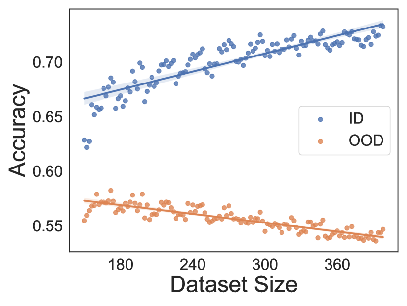
(a) Noisy dataset

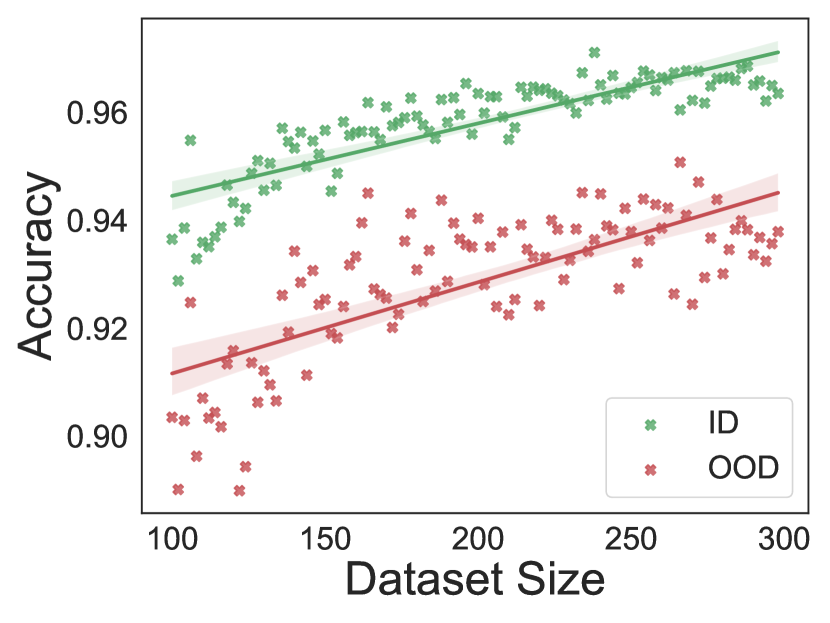
(b) Noiseless dataset

Figure 2: Same setting as Figure 1, increasing dataset size always increases ID accuracy irrespective of label noise, but decreases OOD accuracy in the presence of label noise.

A reader might ask: Can scaling up dataset size resolve the undesirable Accuracy-on-the-wrong-line phenomenon? Recent literature on scaling laws [15, 14] as well as uniform-convergence-based results in classical learning theory suggest that larger datasets are needed to fully benefit from larger models. Even with noise interpolation, larger datasets usually improve generalisation error [5, 6, 24]. However, as Figure 2 suggests, we show that the answer is no. Scaling can adversely impact OOD error, exacerbating the negative correlation between ID and OOD performance. As dataset sizes grow, even a small label noise rate increases the absolute number of noisy points, significantly impacting OOD error, even if it may not always affect ID error.

Contributions. To summarize, the contributions of this work are as follows: (1) We show that Accuracy-on-the-wrong-line can occur in practice and provide experimental results on two image datasets. (2) In a linear setting, we formally prove a lower bound on the difference between per-instance OOD and ID error and characterise sufficient conditions for it to increase. (3) We argue that these conditions are natural properties of learned models, especially for noisy interpolation and in the presence of nuisance features.

Related work. Our work builds on the body of work on the Accuracy-on-the-line phenomenon. Miller et al. [22] first demonstrated empirically that ID and OOD performances exhibit a linear correlation, across many datasets and associated distribution shifts, while Abe et al. [1] showed a similar positive correlation for ensemble models. Liang et al. [20] zoomed in on subpopulation shift–a particular type of distribution shift—and observed a nonlinear "accuracy-on-the-curve" phenomenon. Theoretical analyses by Tripuraneni et al. [41, 40] supported Accuracy-on-the-line in overparameterised linear models. Baek et al. [4] extended the concept to "agreement-on-the-line," showing a correlation between OOD and ID agreement for neural network classifiers. Lee et al. [19] provided theoretical analysis for this phenomenon in high-dimensional random features regression. Kim et al. [16] used these insights to develop a test-time adaptation algorithm for robustness against distribution shift while Eastwood et al. [11] used similar insights to develop a pseudo-labelling strategy to develop robustness across domain shifts. In contrast to these works, our work focuses on the robustness of Accuracy-on-the-line, investigating when it breaks and under what conditions.

Other works have also studied the robustness of Accuracy-on-the-line. Wenzel et al. [44] and Teney et al. [39] empirically suggested that it holds in most but not all datasets and configurations.In particular, Teney et al. [39] also provided a simple linear example where adding spurious features can differently impact ID and OOD risks. Kumar et al. [18] theoretically established an ID-OOD accuracy tradeoff when fine-tuning overparameterised two-layer linear networks. In contrast to all of these works, our work provides both a theoretical analyses and empirical investigations demonstrating the essential impact of label noise and nuisance features in breaking Accuracy-on-the-line. Moreover, we state that it leads to a negative correlation between ID and OOD accuracies, dubbed "Accuracy-on-the-wrong-line." Other lines of work show how label noise affects adversarial robustness [32, 26] and fairness [45, 43]. However, they are not directly related to this work.

2 “Accuracy-on-the-wrong-line” in practice

We first show how a combination of practical limitations in modern machine learning can result in Accuracy-on-the-wrong-line in two real-world computer vision datasets: MNIST [10] and Functional Map of the World (fMoW) [9]. Then in Section 3, we formalise the necessary conditions and provide a theoretical proof showing their sufficiency. In Section 4, we conduct synthetic interventional experiments in a simple linear setting to demonstrate these conditions are indeed sufficient and behave in line with our theoretical results.

2.1 Colored MNIST dataset

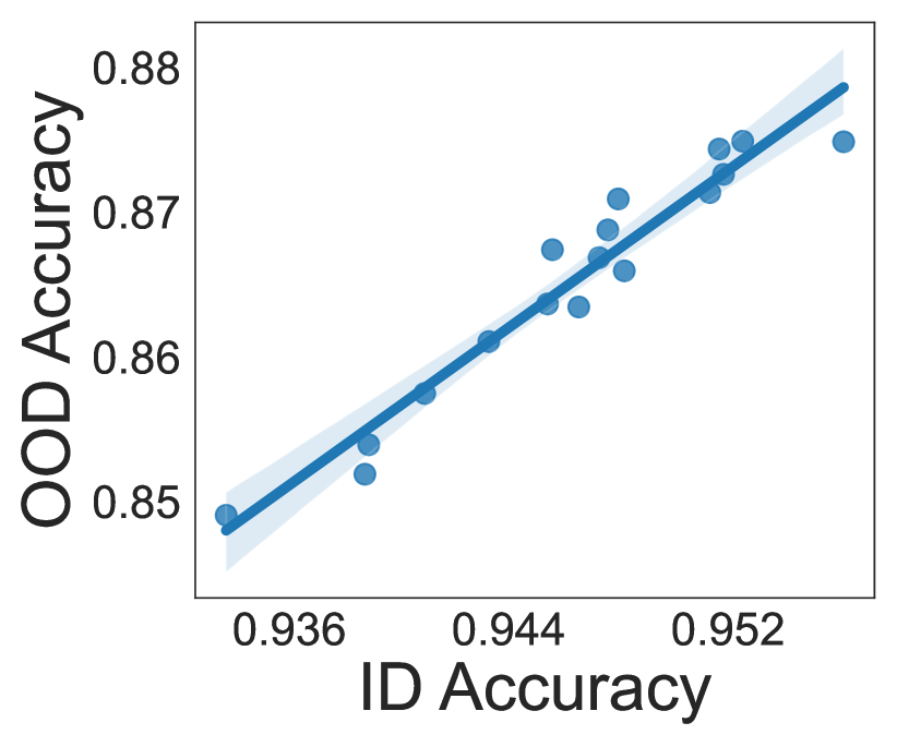
(a) $\eta=0.$

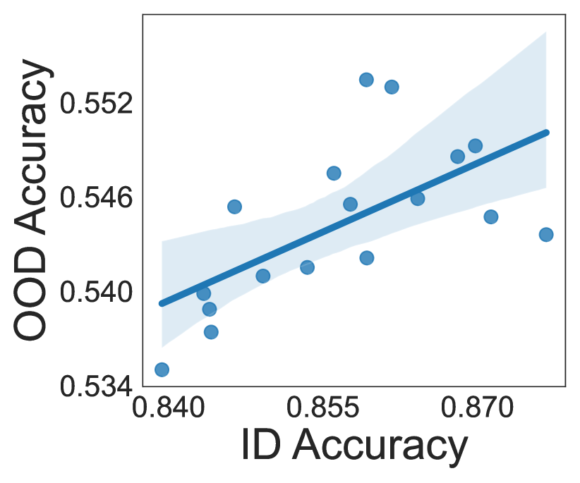
(b) $\eta=0.15$

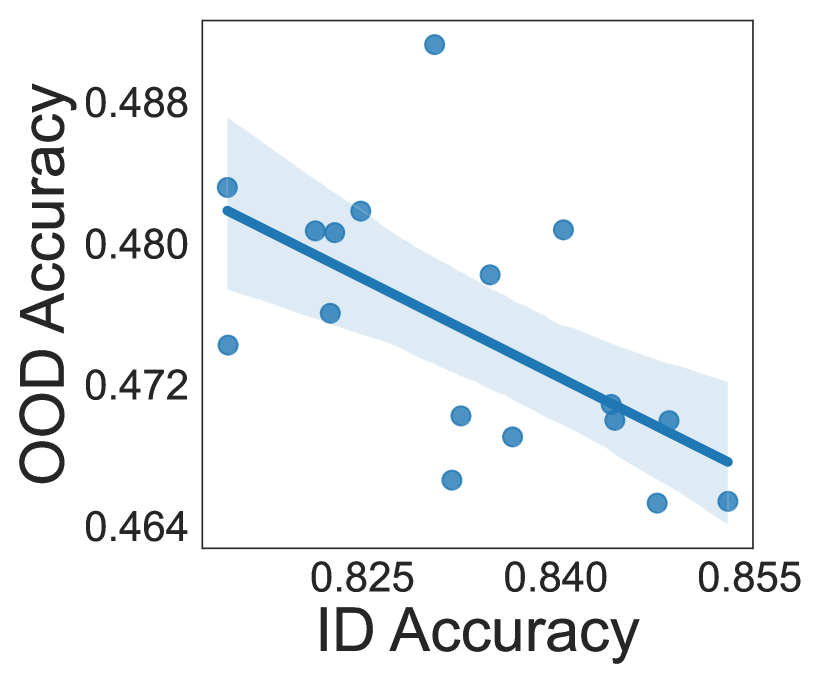
(c) $\eta=0.2$

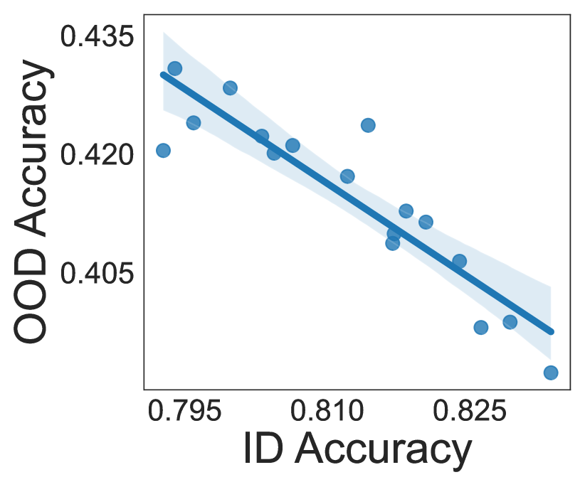
(d) $\eta=0.25$

Figure 3: Each plot shows OOD vs ID accuracy for varying label noise rates $\eta$ on the colored MNIST dataset. Similar to Figure 1, the Accuracy-on-the-line phenomenon degrades with increasing amount of label noise.

We first examine the Colored MNIST dataset, a variant of MNIST, derived from MNIST by introducing a color-based spurious correlation, where the color of each digit is determined by its label with a certain probability. Specifically, digits are assigned a binary label based on their numeric value (less than 5 or not), which is then corrupted with label noise probability $\eta$. The color assigned to each digit is thus correlated with the label with a small probability. A three-layer MLP is then trained on this dataset to achieve zero training error. The model is subsequently tested on a freshly sampled test set from the same distribution but without label noise and with a smaller spurious correlation; see Section B.3 for more details. The accuracy on the training distribution is referred to as the ID accuracy, and the accuracy on the test distribution is referred to as the OOD accuracy.

The results of this experiment are presented in Figure 3. When the amount of label noise is low (Figures 3(a) and 3(b)), the ID and OOD accuracy are positively correlated, whereas they become negatively correlated at higher levels of label noise (Figures 3(c) and 3(d)).

2.2 Functional Map of the World (fMoW) dataset

For the next set of experiments, we use the FMoW-CS dataset designed by Shi et al. [35] based on the original FMoW dataset [9] in WILDS [17, 30]. The dataset contains satellite images from various parts of the world and are labeled according to one of 30 objects in the image. Similar to Colored MNIST, FMoW-CS dataset is constructed by introducing a spurious correlation between the geographic region and the label. Similar to our previous experiments, we also introduce label noise with a probability of 0.5. For the OOD test data, we use the original WILDS [17, 30] test set for FMoW. Further details regarding the dataset are available in Section B.4. To obtain various training runs, we fine-tuned ImageNet pre-trained models, including ResNet-18, ResNet-34, ResNet-50, ResNet-101, and DenseNet121, with various learning rates and weight decays on the FMoW-CS dataset. We also varied the width of the convolution layers to increase or decrease the width of each network. In total, we trained more than 400 models using various configurations and report the results in Figure 4.

Consistent with previous experiments on Colored MNIST, Figure 4(a) shows that when the data comprises label noise and training accuracy is $100\%$, ID and OOD accuracy are inversely correlated. In the absence of label noise, Figure 4(b) shows that the two are positively correlated. These two plots only consider models that fully interpolate the dataset: noisy and noiseless, respectively. To highlight that noisy interpolation is indeed necessary to break the Accuracy-on-the-line phenomenon, we also plot the experiments for those training runs where the data is not fully interpolated in Figure 4(c). This corresponds to early stopping, stronger regularizations, as well as smaller widths. Our results show that in this case, the ID and OOD accuracy are still positively correlated but to a lesser degree than the noiseless setting. We conjecture that this is because even minimizing the cross-entropy loss on noisy labels contributes to this behavior and is strongest when the minimisation leads to interpolation.

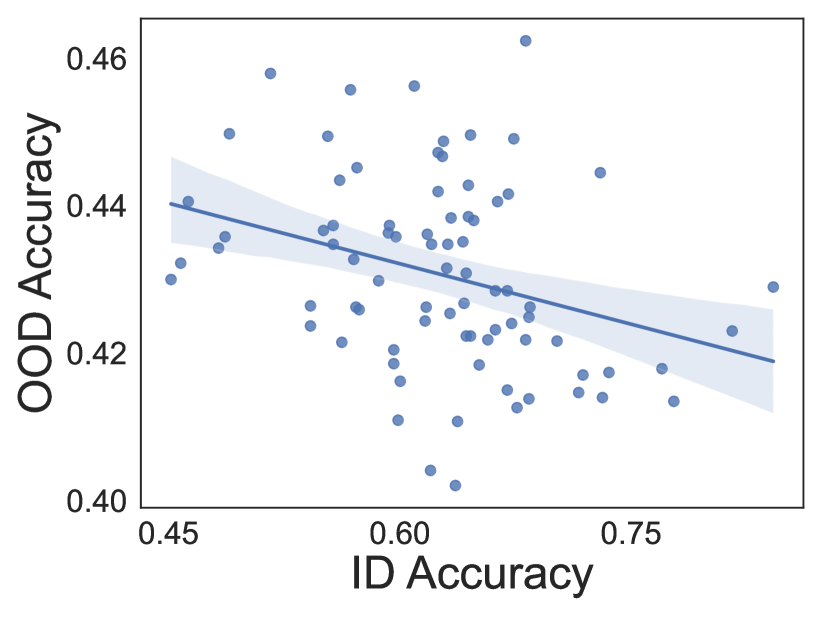
(a) Noisy Interpolation

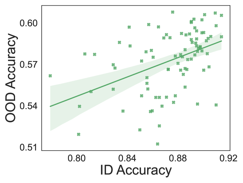
(b) Noiseless Interpolation

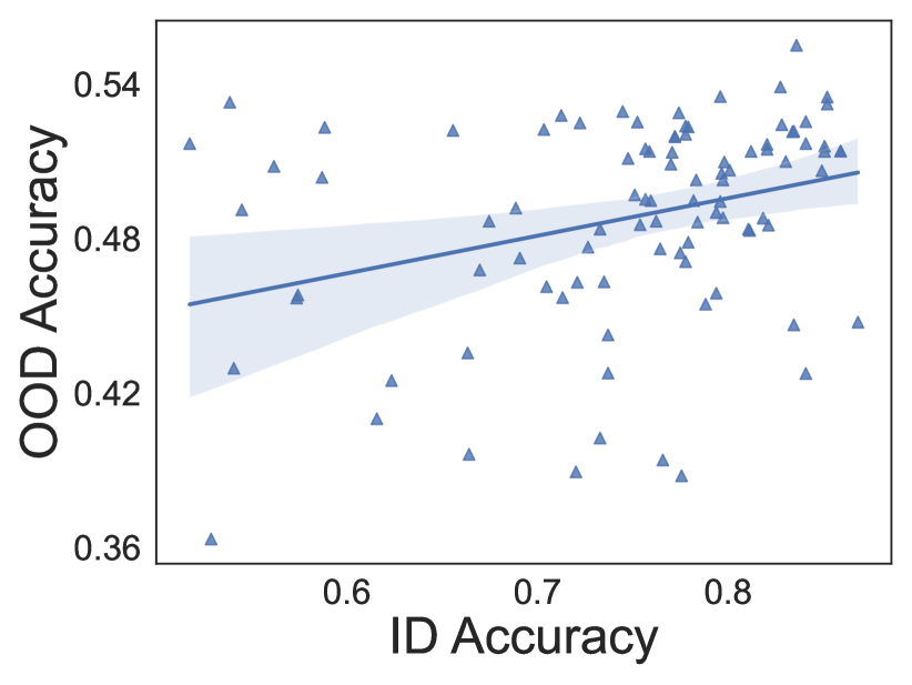
(c) Noisy without interpolation

Figure 4: Experiments on the FMoW domain-correlated dataset with label noise. The noisy dataset (left) shows the Accuracy-on-the-wrong-line phenomenon, while the noiseless dataset (center) shows the Accuracy-on-the-line phenomenon. When the noisy dataset is not interpolated e.g. due to early stopping (right), the Accuracy-on-the-line phenomenon persists.

The results in this section highlight that spurious correlations without label noise are insufficient to enforce Accuracy-on-the-wrong-line. In Appendix B, we also show evidence (Figure 10) that the presence of spurious correlations is necessary in these datasets.

3 “Accuracy-on-the-wrong-line” in theory: sufficient conditions

In this section, we present our main theoretical results to isolate the main factors responsible for breaking the Accuracy-on-the-line phenomenon. First, we define the data distribution $\mu$ in 1 and shift distribution $\Delta$ in 2. The ID error is measured as the expected error on $\mu$ and the OOD error is the expected error on the shifted data i.e. on $x+\delta$ where $x\sim\mu$ and $\delta\sim\Delta$.

Intuitively, the main property of the distribution $\mu$ is that the “signal” and “nuisance” features are supported on disjoint subspaces ($S_{d}$ and $S_{k}$ respectively) and that the shift $\Delta$ does not affect the signal features. Then, 1 lower bounds the difference between OOD and ID error, as a increasing function of the lower bound on nuisance sensitivity of the learned model. Further, in Proposition 3 , we provide a theoretical example, where the lower bound on nuisance sensitivity increases with label noise when the label noise is interpolated. Taken together, Sections 3.3 and 3.4 proves that under high dimensions of nuisance space, and high label noise interpolation negatively impacts OOD error.  We remark that in our theoretical results, we have avoided defining specific data distribution, distribution shifts, or learning algorithms in order to show a result on the general phenomenon and highlight the conditions that give rise to it. We leave it to future work to derive problem and algorithm specific statistical rates of OOD error.

3.1 Data distribution

We model our data distribution $\mu$ to have a few signal features and multiple irrelevant (or nuisance) features. This corresponds to real-world settings where data is usually high dimensional but lies in a low dimensional manifold. We further simplify the setting by restricting this low-dimensional manifold to the linear subspace spanned by the first $d\in{\mathbb{Z}}$ coordinate basis vectors. Formally, for $d,k\in{\mathbb{Z}}$ let $S_{d},S_{k}$ be any two disjoint subsets of $\left\{{1\ldots d+k}\right\}$. Without loss of generality, we assume them to be contiguous i.e. $S_{d}=\left\{{1,\ldots,d}\right\}$ and $S_{k}=\left\{{d+1,\ldots,d+k}\right\}$.

Definition 1.

A distribution $\mu$ on $\mathbb{R}^{d+k}\times\left\{{-1,1}\right\}$ is called a $\left({S_{d},S_{k}}\right)$-disjoint signal distribution with signal and nuisance support $S_{d},S_{k}$ respectively if there exists a linear separator $w\in\mathbb{R}^{d+k}$ with its support exclusively on $S_{d}$ and

$${\mathbb{E}}_{\left({x,y}\right)\sim\mu}\left[{{\mathbb{I}}\left\{{\mathrm{sign}(\left\langle{w},{x}\right\rangle)\neq y}\right\}}\right]=0.$$

We define the shift distribution $\Delta$ as only impacting the nuisance features. This corresponds to widely held assumptions that distribution shifts do not affect the dependence of the label on the signal features. We define such shifts as $S_{d}$-oblivious shifts in 2.

Definition 2.

A shift distribution $\Delta$ is called a $S_{d}$-oblivious shift distribution if the marginal distribution $\Delta_{S_{d}}$ on the support $S_{d}$ is concentrated fully on $\mathbf{0}_{d}$, i.e.

$$\Delta_{S_{d}}\left({\mathbf{0}_{d}}\right)=1.$$

In short, both definitions assume that there are two orthogonal subspaces. For theoretical modelling, we consider that the signal subspace and the nuisance subspace are exactly disjoint in the standard coordinate basis. While this may not hold in the original data space in practice, this usually holds in the latent space as a few components in the latent space are sufficient to solve the problem at hand. We regard those components as the signal space and the rest as the nuisance subspace. The assumption that the $S_{d}$-oblivious shift distribution has no mass on the signal space reflects a natural assumption about distribution shifts: they do not affect the causal factors in the data.

3.2 Properties of learned model

The above definitions for ID and OOD data alone do not provide sufficient conditions to break the Accuracy-on-the-line behavior. These definitions align with realistic settings, such as the sparsity of the true labeling function and distribution shifts orthogonal to the features in the signal space. Consequently, real-world experiments on the Accuracy-on-the-line phenomenon already explore these conditions. Therefore, we next define three conditions on the learned model that we identify as sufficient to break this phenomenon.

Let $\widehat{w}\in\mathbb{R}^{d+k}$ be the learned sparse linear classifier with support $S$. Let $\mu,\Delta$ be any $(S_{d},S_{k})$-disjoint signal distribution and $S_{d}$-oblivious shift distribution as defined in 1 for some $S_{d},S_{k}$, and define $\nu={\mathbb{E}}\left[{\Delta}\right]$ as the mean of $\Delta$. Then, we state the following conditions on $\widehat{w}$.

• Condition C1: “Bounded sensitivity" of $\hat{w}$ on nuisance subspace assumes there exists $M,\tau\geq 0$ s.t.

  $$M\geq\max_{i\in S_{k}\cap S}|\hat{w}_{i}|\geq\min_{i\in S_{k}\cap S}|\hat{w}_{i}|\geq\tau.$$ (C1)

• Condition C2: “Negative Alignment" of $\hat{w}$ with mean of shift $\nu$ assumes there exists $\gamma>0$ s.t.

  $$\gamma\leq-\frac{\sum_{i\in S_{k}\cap S}\hat{w}_{i}\nu_{i}}{\mathrm{\left\lVert\widehat{w}_{S_{k}\cap S}\right\rVert}_{1}}.$$ (C2)

• Condition C3: “Small Margin" of $\hat{w}$ assumes that for all $x$ s.t. $\left\langle{\widehat{w}},{x}\right\rangle>0$, the following holds

  $$\left\langle{\hat{w}},{x}\right\rangle\leq\tau\gamma\left|{S_{k}\cap S}\right|.$$ (C3)

3.3 Main theoretical result

Now, we are ready to state the main result. In 1, we provide a lower bound on the OOD error corresponding to a fixed $x$ where the randomness is over the sampling of the shift $\delta\sim\Delta$.

Theorem 1.

For any $S_{d},S_{k}$ let $\mathcal{D}$ be a $(S_{d},S_{k})$-disjoint signal distribution, and $\Delta$ be a $S_{d}$-oblivious shift distribution where each coordinate is an independent subgaussian with parameter $\sigma$.

Then, for any $x\in\mathrm{dom}\left({\mu}\right)$ and $\widehat{w}\in\mathbb{R}^{d+k}$ with support $S$ such that $\widehat{w}$ satisfies Conditions C1, C2, and C3, we have $\mathrm{Pr}_{\delta}\left({\left\langle{\hat{w}},{x+\delta}\right\rangle\leq 0}\right)\geq 1-e^{-\Gamma}$ where

$$\Gamma=\frac{\left|{S_{k}\cap S}\right|\left({\tau\gamma-\nicefrac{{{\mathcal{C}}}}{{\left|{S_{k}\cap S}\right|}}}\right)^{2}}{2\sigma^{2}M^{2}}.$$ (1)

for all $x\in\mathrm{dom}\left({\mu}\right)$ where $\left\langle{\widehat{w}},{x}\right\rangle\geq 0$ and ${\mathcal{C}}=\max_{\left\langle{\widehat{w}},{x}\right\rangle\geq 0}\left\langle{\widehat{w}},{x}\right\rangle$.

1 proves that for all (positively) correctly classified points, the probability of misclassification under the OOD perturbation $\delta$ increases with $\Gamma$. In particular, $\Gamma$ scales with the nuisance sensitivity $\tau$ and nuisance density $\left|{S_{k}\cup S}\right|$. Our experiments later show that increasing data size, which leads to lower ID error, in fact increases nuisance density, which as 1 suggest, leads to larger OOD error.

The proof of the theorem is based on applying a Chernoff-style bound on a weighted combination of $k$ sub-gaussian random variables; see Appendix A for the full proof. 1 captures a broad class of distribution shifts, including bounded and normal distributions. The results can also be extended to other shifts with bounded moments but we omit them here as they add more mathematical complexity without additional insights. In particular, under the conditions of 1, for some $\sigma>0,\nu\in\mathbb{R}^{d+k}$ where $\nu$ satisfies A2, consider either:

• Gaussian Shifts: Each $\delta_{i}$ for $i\in S_{k}\cap S$ is independently distributed as ${\mathcal{N}}(\nu_{i},\sigma^{2})$, or

• Bounded Shifts: Each $\delta_{i}$ for $i\in S_{k}\cap S$ satisfies $\left|{\delta_{i}-\nu_{i}}\right|\leq\sqrt{3}\sigma$.

Then, the probability that $\widehat{w}$ misclassifies $x$ which satisfies (C3) under the shift $\delta$ is bounded by the same expression as in Equation 1.

3.4 Understanding and relaxing conditions

We next argue why these conditions are merely abstractions of phenomena already observed in practice, as opposed to strong synthetic constraints absent in applications. In addition, we also show how some of these conditions can be significantly relaxed.

Relaxing Condition (C2) and (C3). Our setting is not restricted to only discussing samples from one class, balanced classes, or cases where all data points have small margins. In this section, we relax Condition (C2) and (C3) to allow for imbalanced classes and for some data points to have large margins. Condition C3 requires that for all data points that are positively classified, the margin of classification is bounded from above. Note that this is not a limitation of our result. A simple corollary (Corollary 2) states the proportion of $\mu$ for which this holds directly affects the proportion for which the OOD performance is poor. We use the notation $\rho$ in Equation C4 to characterise the fraction of the dataset classified positively (or negatively, whichever yields a higher $\rho$) by $\widehat{w}$ with a margin that is less than half of the maximum allowed margin.

Condition (C2) requires that the distribution shift should not orthogonal to $\widehat{w}$. This is not a strict requirement, as exact orthogonality of $\nu$ with $\hat{w}$ is a very unlikely setting, and even slight misalignment will suffice for our result. Here, we show that if the shift distribution is a mixture of multiple components with a combination of positive and negative alignments, our result extends to that setting. Consider a new shift distribution $\Delta^{\prime}$, which is a mixture of two shift distributions $\Delta_{1}$ and $\Delta_{-1}$ with mixture coefficients $c_{1}$ and $c_{-1}$, respectively. Now note that at least one of the two-component shift distributions will likely satisfy Condition (C2) with $\widehat{w}$ or $-\widehat{w}$. Assume, $\Delta_{1}$ satisfies condition (C2) with $\gamma_{1}$, and $\Delta_{-1}$ satisfies the same condition by replacing $\widehat{w}$ with $-\widehat{w}$ for $\gamma_{-1}$.

As shown in Corollary 2, when the distribution becomes more class-imbalanced and a large fraction of data points have small margins and at least one of the distributions has a large negative alignment $\gamma$, the parameter $\rho$ increases, thereby increasing the probability of misclassification.

Corollary 2.

Define $S_{d},S_{k}$, and $\mu$ as in 1 and $\Delta^{\prime}$ as described above. Consider any $\widehat{w}\in\mathbb{R}^{d+k}$ with support $S$ such that $\widehat{w}$ satisfies Conditions C1 and C2. Define

$$\rho=\max_{\hat{y}\in\left\{{-1,1}\right\}}\mathrm{Pr}_{x\sim\mu}\left[{{\mathbb{I}}\left\{{\hat{y}\left\langle{\widehat{w}},{x}\right\rangle\geq 0}\right\}\cdot{\mathbb{I}}\left\{{\hat{y}\left\langle{\widehat{w}},{x}\right\rangle\leq\frac{\tau\gamma_{\hat{y}}\left|{S_{k}\cap S}\right|}{2}}\right\}}\right].$$ (C4)

Then, we have

$$\mathrm{Pr}_{x,\delta}\left({\left\langle{\hat{w}},{x+\delta}\right\rangle\neq\left\langle{\widehat{w}},{x}\right\rangle}\right)\geq\rho_{c}\sum_{i\in\{-1,1\}}c_{i}\left({1-\exp\left\{{-\frac{\left|{S_{k}\cap S}\right|\tau^{2}\gamma_{i}^{2}}{8\sigma^{2}M^{2}}}\right\}}\right).$$

The above result shows how the OOD error adaptively depends on various properties of the learned classifier and shift distribution. It shows that the OOD error increases with the increase in the density of $\widehat{w}$ in the nuisance subspace, i.e. $\left|{S_{k}\cap S}\right|$, as well as the ratio of the minimum and maximum spurious sensitivity $\frac{\tau}{M}$, from Condition C1. Second, the increase in the negative alignment $\gamma$ increases the OOD error and it depends on which class has the worse parameters. Finally, we note that $1-\rho$ upper bounds ID error. Therefore, while a larger $\rho$ leads to a larger lower bound on the OOD error, it leads to a smaller upper bound on the ID error— a reflection of the Accuracy-on-the-wrong-line behaviour.

Understanding Condition (C1). Condition (C1) describes the condition that the learned classifier has moderately large values in its support on the nuisance subspace. We provide an example in Proposition 3 to show that this naturally occurs when interpolating label noise. Consider a min-$\ell_{2}$-interpolator that solves the following optimization problem given a dataset $(X,Y)\in\mathbb{R}^{n\times d}\times\mathbb{R}^{n}$,

$$\min_{w\in\mathbb{R}^{d}}\mathrm{\left\lVert w\right\rVert}_{2}\quad\mathrm{s.t.}~{}Xw=Y.$$

Consider a simple linear model with a single signal feature $Y=\xi\odot\left\langle{X},{w^{\star}}\right\rangle$ where $w^{\star}=\left({1,0,\ldots,0}\right)$. Here, $X$ is a $d$-dimensional dataset of size $n$ with signal feature $X_{1}\sim{\mathcal{N}}(\upsilon\mathbf{1}_{n},I_{n})$ and the remaining $d-1$ nuisance features $X_{2:d}\sim{\mathcal{N}}(0,I_{n})$. The label noise $\xi\in\mathbb{R}^{n}$ follows the distribution $\pi$ and $\odot$ denotes the Hadamard product. When $\xi$ is a Bernoulli random variable on the set $\left\{{-1,1}\right\}$, it captures the setting of uniformly random label flip.

Proposition 3 (Informal).

If for $d=\Omega\left({\log n}\right)$, some constant $C>0$, and $\beta\in(0,1)$, the noise distribution $\pi$ satisfies $\mathrm{Pr}\left[{\mathrm{\left\lVert X_{2:d}^{+}\xi\right\rVert}_{2}>C}\right]\geq 1-\beta$, where $A^{+}$ is the pseudo-inverse of $A$, then with probability at least $0.9-\beta$, the min-$\ell_{2}$-interpolator $\hat{w}$ on the noisy dataset $(X,Y)$ satisfies

$$\mathrm{\left\lVert\hat{w}_{2:d}\right\rVert}_{\infty}=\Omega\left({C}\right).$$

While Proposition 3 only considers multiplicative label noise for simplicity of the analysis, similar results also hold for additive label noise models. Proposition 3 also captures the properties of label noise that are sufficient to increase the sensitivity of the nuisance features. It suggests that a label noise distribution, whose (noisy) labels are nearly orthogonal to the nuisance subspace (indicated by large $C$ and small $\beta$), induces small nuisance sensitivity. For example, a noiseless setting is equivalent to the noise distribution where $\mathrm{Pr}_{\xi\sim\mu}\left[{\xi=\mathbf{1}_{n}}\right]=1$. Then, standard concentration bounds on $X_{2:d}$ imply that $C$ must be small while $\beta$ must be large, leading to a vacuous bound. Therefore, Proposition 3 implies that the lower bound on nuisance sensitivity is much smaller in the noiseless setting.

Next, we verify these properties on a simple learning problem in Section 4. Our experiments show that increasing dataset size can naturally increase $\left|{S_{k}\cap S}\right|$ and $\tau$, thereby leading to a larger OOD error. Conversely, increasing the dataset size will also lead to a lower ID error. Together, this demonstrates an inverse correlation between ID and OOD error, displaying Accuracy-on-the-wrong-line.

4 Experimental ablation of sufficient conditions in linear setting

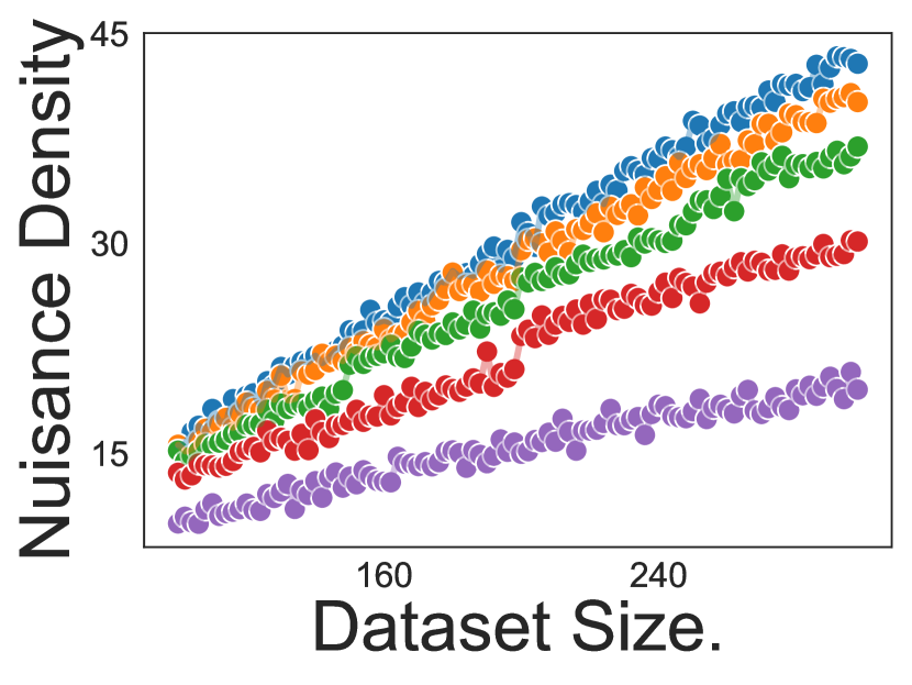
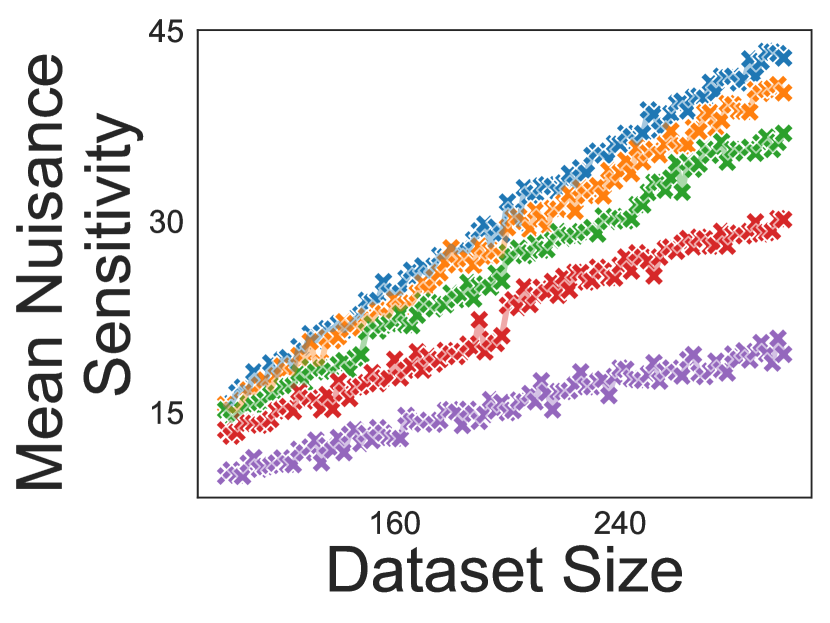
(a) Nuisance Sensitivity

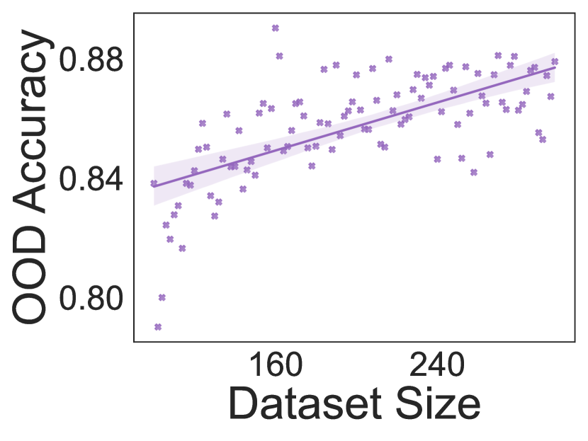
(b) OOD Accuracy

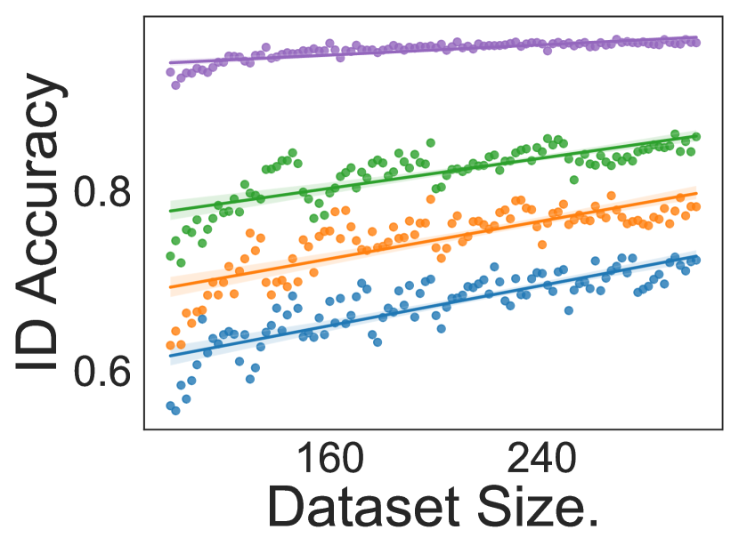
(c) ID Accuracy

Figure 5: Figure 5(a) shows as the amount of label noise increases, nuisance sensitivity as well as the nuisance density increases faster with larger dataset sizes. This leads to worse OOD accuracy as shown in Figure 5(b). However, ID accuracy still increases with dataset size as shown in Figure 5(c).

In this section, we conduct experimental simulations to corroborate our theory by synthetically varying conditions (C1), (C2), and (C4) as well as label noise rate and dataset sizes. The data distribution is $300$-dimensional with one signal feature and the remain nuisance features, a sparse setting often considered in the literature; See Section B.1 for a detailed discussion of the data distribution. The default label noise rate is $0.2$ unless otherwise mentioned and the default dataset size is $300$ unless otherwise mentioned. We train a $\ell_{1}$-penalised logistic regression classifier with coefficient $0.1$ on varying dataset sizes. In short, our experiments show that all three conditions hold for this learned model in the presence of label noise and corroborates our theory regarding how these problem parameters affect the OOD and Accuracy-on-the-line phenomenon.

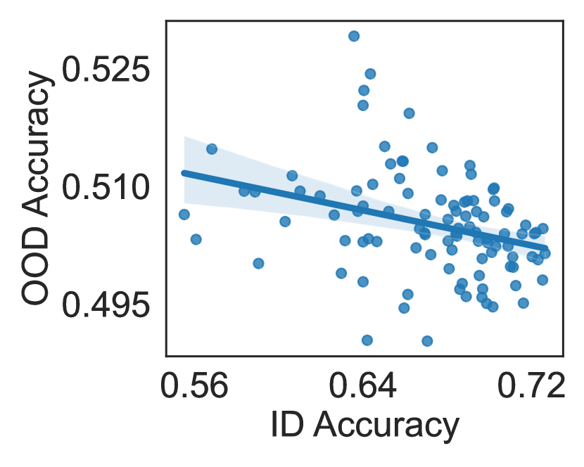
$\eta=0.2$

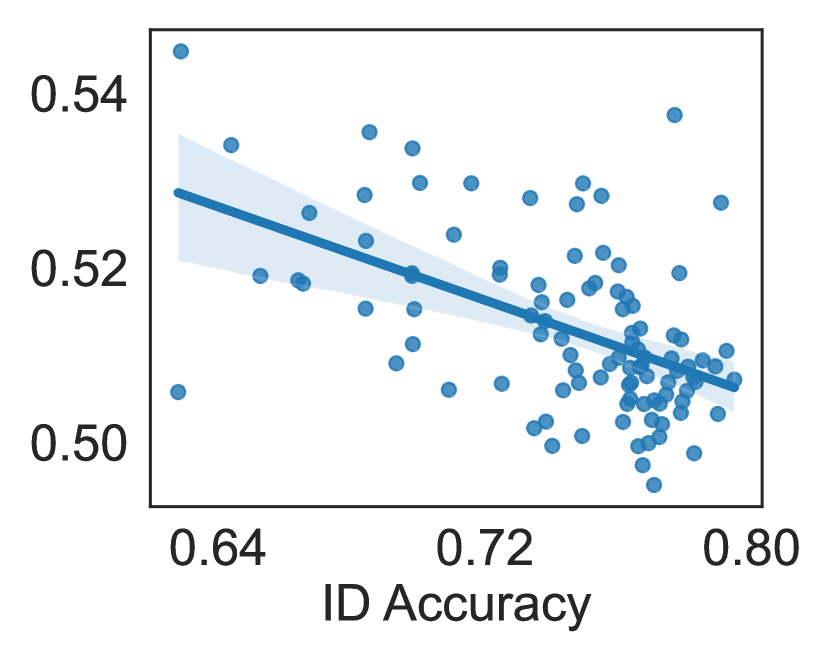
$\eta=0.15$

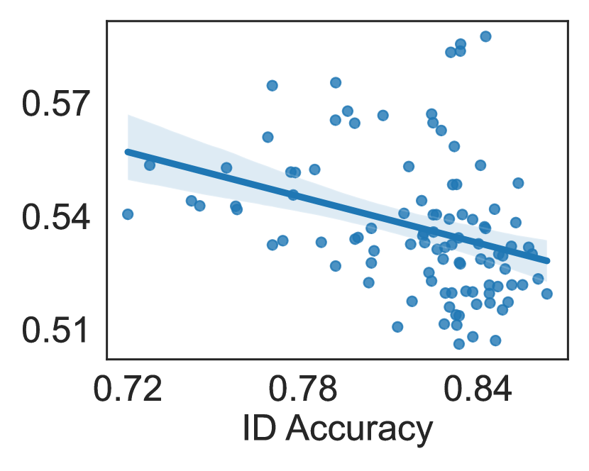
$\eta=0.1$

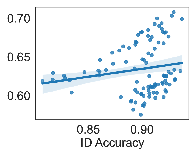
$\eta=0.05$

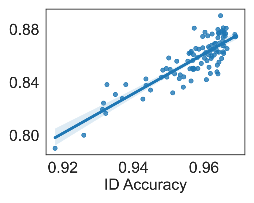
$\eta=0$

Figure 6: Accuracy-on-the-line behaviour degrades increasing with increasing amount of label noise.

(C1): Spurious Sensitivity of the Learned Model. We begin by examining the sensitivity of the learned model $\widehat{w}$ in the nuisance subspace. Condition (C1) states that the non-zero components are bounded both from above and below. While regularisation naturally imposes the upper bound, the lower bound is less common. A key contribution of this work is the demonstration that this occurs under noisy interpolation, i.e., models that achieve zero training error in the presence of label noise. Intuitively, when some labels in the training dataset are noisy, the signal subspace cannot be used to “memorise” them. Consequently, covariates in the nuisance subspace are necessary to memorise these labels, thereby increasing the magnitude of these covariates. As the amount of label noise increases, more covariates in the nuisance subspace exhibit this behaviour. We corroborate this intuition using $\ell_{1}$-penalised logistic regression in experimental simulations, as shown in Figure 5(a).

Figure 5(a) illustrates that, with higher levels of label noise, the nuisance density and mean nuisance sensitivity increase more rapidly as the dataset size grows.  1 predicts that an increase in nuisance sensitivity leads to poorer OOD accuracy, which is confirmed in Figure 5(b) (center). However, Figure 5(b) (left) demonstrates that this behaviour is not observed in the absence of label noise; OOD accuracy still improves with an increasing dataset size.  Figure 5(c) reveals that ID accuracy increases with larger datasets, thereby creating a distinction between the behaviour of ID and OOD accuracy in the presence of label noise. This distinction underpins the central observation of our paper, as illustrated in Figure 6. For $\eta=0$ (no label noise), ID and OOD accuracy are linearly correlated as noted in several prior studies [22]. Conversely, as $\eta$ increases, the two accuracies become (nearly) inversely correlated, resulting in the Accuracy-on-the-wrong-line behaviour.

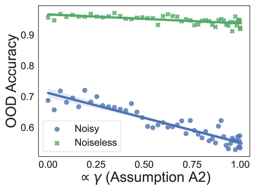
(a) OOD Accuracy vs $\gamma$

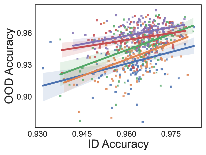
(b) Noiseless

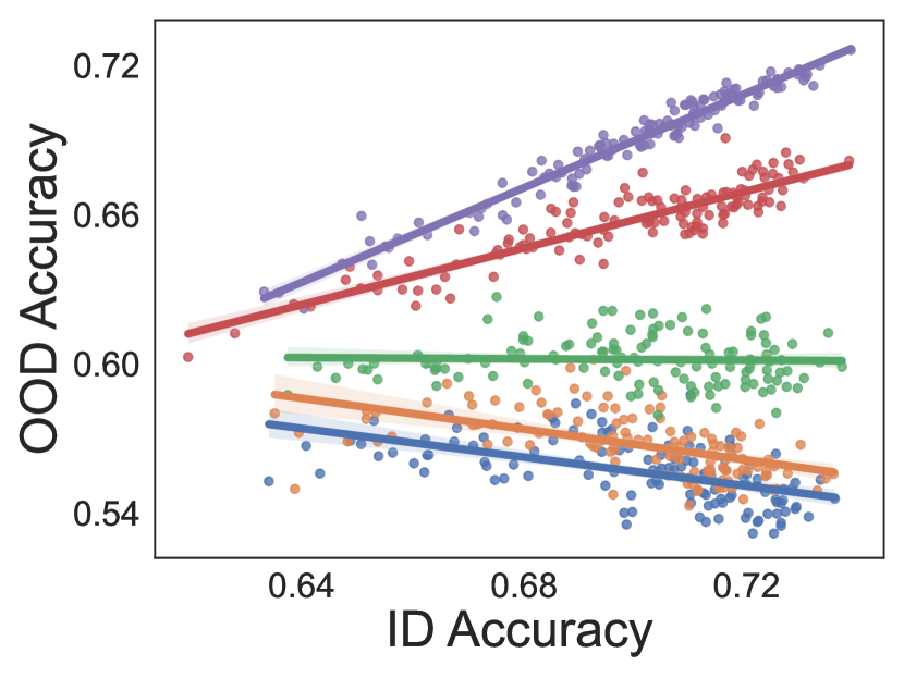
(c) Noisy

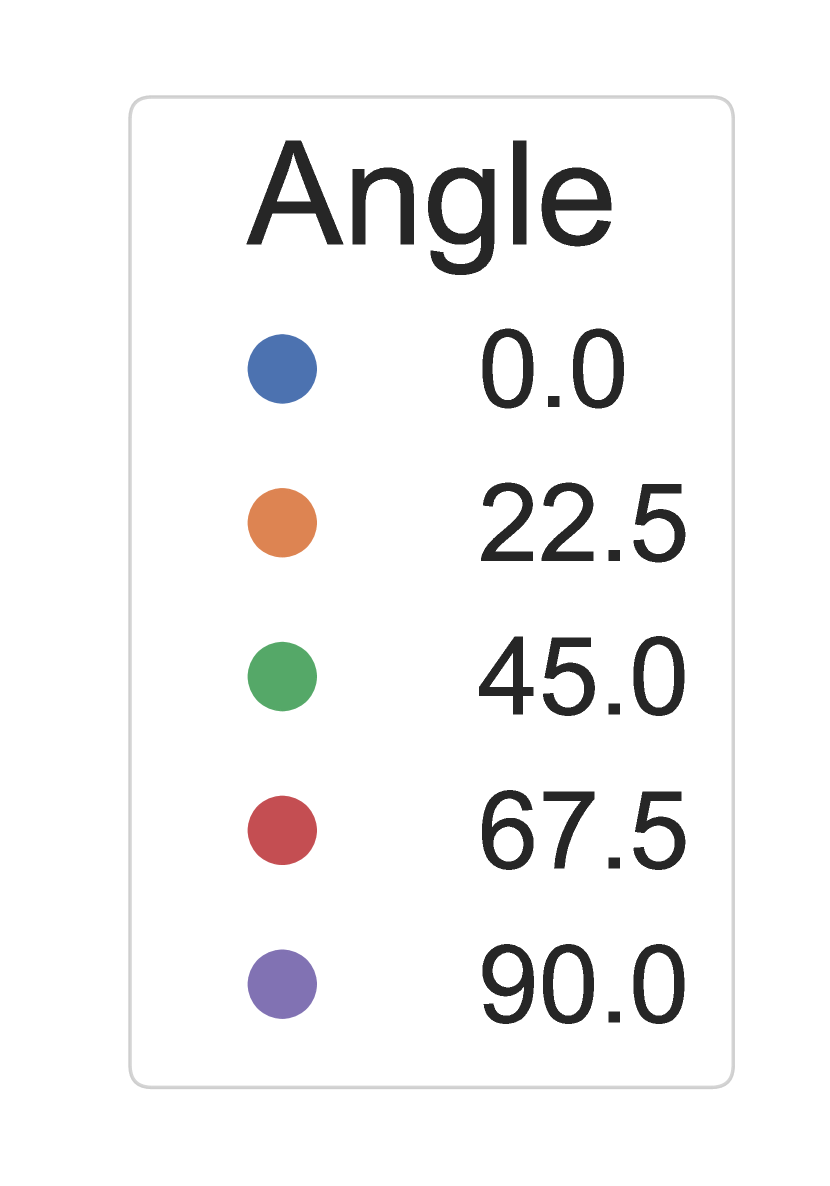
Figure 7:  Figure 7(a) shows that as $\gamma$ increases, the OOD accuracy decreases for the noisy setting but remains relatively unchanged for the noiseless setting. Figure 7(b) shows that a large or small angle ($\cos\left({\mathrm{Angle}}\right)=\gamma$) does not have any impact on breaking the Accuracy-on-the-line phenomenon. On the other hand, when angle is close to $0\mathrm{°}$ i.e. $\widehat{w}$ and $\nu$ in C2 are fully mis-aligned, the accuracy-on-the-wrong line behaviour is the strongest. The phenomenon slowly transforms to Accuracy-on-the-line as the angle approaches $90\mathrm{°}$ degrees.

(C2): Mis-alignment of Learned Model with Shift distribution. The next condition on $\widehat{w}$ requires that the mean $\nu$ of the shift distribution $\Delta$ is misaligned. Mathematically, this requires that the dot product $\langle\widehat{w},\nu\rangle$ is negative. Intuitively, this ensures that the term $\langle\widehat{w},\delta\rangle$, where $\delta\sim\Delta$, is sufficiently negative to flip the decision of the classifier. In 1, the alignment is measured using the quantity $\gamma$. In Figure 7(a), we synthetically vary $\gamma$ (represented by the angle between $\nu$ and $-\widehat{w}$) by controlling the projection of $\nu$ on $-\widehat{w}$ and evaluate the OOD accuracy in the presence and absence of noise, respectively. The simulation shows that with increasing alignment between $\nu$ and $-\widehat{w}$, OOD accuracy decreases sharply for the noisy setting but remains relatively stable for the noiseless setting.

In Figures 7(b) and 7(c), we show how the Accuracy-on-the-line behaviour is affected by changing the alignment $\gamma$. For the noiseless setting, irrespective of $\gamma$, OOD accuracy remains positively correlated with ID accuracy. However, for the noisy setting, when the alignment is high (i.e., the angle is less than $45^{\circ}$), we observe that OOD accuracy is inversely correlated with ID accuracy, but they become more positively correlated as the angle increases. This highlights the necessity of our second condition, which requires a misalignment between the shift and the learned parameters. This also highlights that perfect misalignment is not strictly necessary for breaking Accuracy-on-the-line.

(C4): Significant fraction of points have low margin. The final property of the learned classifier necessary for the Accuracy-on-the-wrong-line phenomenon is that a significant portion of the distribution, correctly classified by $\widehat{w}$, has a small margin. This is captured in C4. Corollary 2 suggests that the probability mass of points under distribution $\mu$ whose margin $\langle\widehat{w},x\rangle$ is less than $\gamma\tau|S_{k}\cap S|\approx\gamma\|\widehat{w}_{S_{k}\cap S}\|_{1}$ is roughly equal to the probability mass of points under $\mu$ that are vulnerable to misclassification under the distribution shift. Practically, a point classified correctly with a large margin is likely robust to distribution shifts. However, it is typically the case that not all points are classified with an equally large margin, and some points are closer to the margin than others. We highlight that as long as this is true, Accuracy-on-the-wrong-line will continue to hold.

To validate this experimentally, we consider the distribution of ID margin $\langle\widehat{w},x\rangle$ for $x\sim\mu$ and plot its CDF in Figure 8 (blue line). Then, we measure the term $\gamma\tau|S_{k}\cap S|$ and plot it as a vertical red dashed line. The intersection of this red line with the CDF (blue) represents the probability mass of points under $\mu$ whose margin is sufficiently small to be vulnerable to the distribution shift. We plot the empirical OOD error for this model using the horizontal green dashed line and repeat this experiment for multiple dataset sizes, each represented in one box in Figure 8. Our simulations clearly show that the theoretically predicted quantity closely approximates the true OOD error.

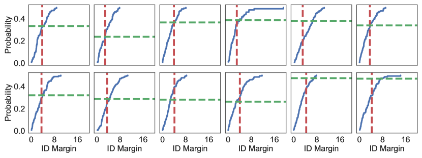
Figure 8: Blue line is the CDF of the ID margin i.e. $\left\langle{\widehat{w}},{x}\right\rangle$ for points $x$ classified positively by $\widehat{w}$. The red vertical line indicates the theoretical quantity in the RHS of Condition (C4) i.e. proportional to $\tau\gamma\left|{S_{k}\cap S}\right|$. The green line shows the OOD error. Matching the result of Corollary 2, this simulation shows that the fraction of positively classified points whose margin is less than $\tau\gamma\left|{S_{k}\cap S}\right|$ is very close to the true OOD error of that model. Each plot here represents a different run on a different-sized dataset.

5 Implications and conclusion

To summarise, our work argues that interpolation of label noise and presence of nuisance features break the otherwise positively correlated relationship between ID and OOD accuracy. In support of this argument, we provide experimental evidence with realistic datasets, theoretical results to isolate the sufficient conditions, and synthetic simulation to corroborate the theoretical assumptions.

Future Work This raises several questions about the widely prevalent practice of preferring large but noisy datasets over smaller cleaner datasets. We hope future work will work towards striking the right balance between size and quality of datasets, keeping in mind their impact on trustworthiness metrics like OOD accuracy. Proposition 3 shows a sufficient condition for when label noise can increase the nuisance sensitivity; however this result is restricted to $\min~{}\ell_{2}$ interpolators. It is an interesting question to consider what label noise models (e.g. uniform label flip) and inductive biases of the learning algorithm (e.g. $\min~{}\ell_{p}$) [2, 7] can aggravate or mitigate this phenomenon. It is also interesting to investigate what other factors (e.g. spurious correlation alone [39]) can lead to similar behaviours. Finally, other works have proposed approaches to mitigate memorisation of label noise [47, 31], selectively learning signal features [3, 27], unlearning the effect of manipulated data [13, 38], and improving robustness towards adversarial corruptions [21, 37]. The possible impact of these techniques on preventing Accuracy-on-the-wrong-line is an interesting line of future work.

Appendix A Proofs

In this section, we provide the proofs of 1 and Corollary 2. Then, we state and prove 5, which is the full version of Proposition 3.

See 1

Proof.

WLOG consider $x\in\mathrm{dom}\left({\mu}\right)$ such that $\left\langle{\widehat{w}},{x}\right\rangle\geq 0$. Then, define the event $E:=\left\{{\delta\in\mathbb{R}^{d+k}:\left\langle{\widehat{w}},{x+\delta}\right\rangle\leq 0}\right\}$ for which we need to bound $\mathrm{Pr}\left[{E}\right]$. Decomposing the dot product affected by the shift, $\left\langle{\widehat{w}},{x+\delta}\right\rangle=\left\langle{\widehat{w}},{x}\right\rangle+\left\langle{\widehat{w}},{\delta}\right\rangle$. Given $\Delta$ is $S_{d}$-oblivious, $\delta$ contributes only from the coordinates in $S_{k}\cap S$. Then, we can simplify the probability as

$$\mathrm{Pr}\left[{E}\right]=\mathrm{Pr}_{\delta}\left[{\left\langle{\hat{w}},{x+\delta}\right\rangle\leq 0}\right] =\mathrm{Pr}_{\delta}\left[{\sum_{i\in S_{k}\cap S}\hat{w}_{i}\delta_{i}\leq-\left\langle{\widehat{w}},{x}\right\rangle}\right]$$ (2)

$$=1-\mathrm{Pr}_{\delta}\left[{\sum_{i\in S_{k}\cap S}\hat{w}_{i}\delta_{i}\geq-{\mathcal{C}}}\right]$$

$$\geq 1-\inf_{\lambda\geq 0}e^{\lambda{\mathcal{C}}}~{}{\mathbb{E}}\left[{e^{\lambda\sum_{i\in S_{k}\cap S}\hat{w}_{i}\delta_{i}}}\right]$$

As each $\delta_{i}$ is independently distributed with subgaussian parameter $\sigma$ and mean $\nu_{i}$, by the properties of subgaussian random variables, for $\lambda\geq 0$, the moment generating function (MGF) of $\delta_{i}$ yields

$${\mathbb{E}}\left[{e^{\lambda\delta_{i}}}\right]\leq e^{\lambda\nu_{i}+\frac{\lambda^{2}\sigma^{2}}{2}}$$

Subsituting this into the Chernoff bound in Equation 2, we obtain

$$\mathrm{Pr}\left[{E}\right] \geq 1-\inf_{\lambda\geq 0}e^{\lambda{\mathcal{C}}+\lambda\left\langle{\widehat{w}},{\nu}\right\rangle+\lambda^{2}\sum_{i\in S_{k}\cap S}\nicefrac{{\widehat{w}_{i}^{2}\sigma^{2}}}{{2}}}$$ (3)

$$\geq 1-\inf_{\lambda\geq 0}e^{\lambda{\mathcal{C}}+\left|{S_{k}\cap S}\right|\left({-\lambda\tau\gamma+\lambda^{2}M^{2}\sigma^{2}}\right)}$$

where the last inequality uses Assumptions A1 and A2. Solving the above optimisation to obtain the optimal lambda yields

$$\lambda=\frac{\tau\gamma\left|{S_{k}\cap S}\right|-{\mathcal{C}}}{\sigma^{2}M^{2}}$$

Note that assumption A3 ensures that this term is positive. Substituting this back into Equation 3 and simplifying the resultant expression yields the following probability bound

$$\mathrm{Pr}\left({\left\langle{\hat{w}},{x+\delta}\right\rangle\leq 0}\right)\geq 1-\exp\left\{{-\frac{\left|{S_{k}\cap S}\right|\left({\tau\gamma-\nicefrac{{{\mathcal{C}}}}{{\left|{S_{k}\cap S}\right|}}}\right)^{2}}{2\sigma^{2}M^{2}}}\right\}.$$

∎

Here, we provide a full version of Corollary 2. Specifically, Corollary 2 is a special case of Corollary 4 with $c=1/2$.

Corollary 4.

Define $S_{d},S_{k}$, and $\mu$ as in 1 and $\Delta^{\prime}$ as described above. Consider any $\widehat{w}\in\mathbb{R}^{d+k}$ with support $S$ such that $\widehat{w}$ satisfies Conditions C1 and C2. For any $0\leq c\leq 1$ define

$$\rho_{c}=\max_{\hat{y}\in\left\{{-1,1}\right\}}\mathrm{Pr}_{x\sim\mu}\left[{{\mathbb{I}}\left\{{\hat{y}\left\langle{\widehat{w}},{x}\right\rangle\geq 0}\right\}\cdot{\mathbb{I}}\left\{{\hat{y}\left\langle{\widehat{w}},{x}\right\rangle\leq c\tau\gamma_{\hat{y}}\left|{S_{k}\cap S}\right|}\right\}}\right].$$ (C4)

Then, we have

$$\mathrm{Pr}_{x,\delta}\left({\left\langle{\hat{w}},{x+\delta}\right\rangle\neq\left\langle{\widehat{w}},{x}\right\rangle}\right)\geq\rho_{c}\sum_{i\in\{-1,1\}}c_{i}\left({1-\exp\left\{{-\frac{\left|{S_{k}\cap S}\right|\tau^{2}\gamma_{i}^{2}\left({1-c}\right)^{2}}{2\sigma^{2}M^{2}}}\right\}}\right).$$

Proof.

Let $y_{\max}$ denote the value of $\hat{y}$ that achieve $\rho_{c}$, ie.

$$y_{\max}=\mathop{\mathrm{argmax}}_{\hat{y}\in\left\{{-1,1}\right\}}\mathrm{Pr}_{x\sim\mu}\left[{{\mathbb{I}}\left\{{\hat{y}\left\langle{\widehat{w}},{x}\right\rangle\geq 0}\right\}\cdot{\mathbb{I}}\left\{{\hat{y}\left\langle{\widehat{w}},{x}\right\rangle\leq c\tau\gamma_{\hat{y}}\left|{S_{k}\cap S}\right|}\right\}}\right].$$

For simplicity, we also denote the event ${\mathbb{I}}\left\{{\left\langle{\hat{w},x+\delta}\right\rangle\neq\left\langle{\hat{w},x}\right\rangle}\right\}$ as ${\mathcal{E}}_{\textrm{err}}$. Then, the goal of the proof is to lower bound $\mathrm{Pr}_{x,\delta\sim\Delta^{\prime}}\left({{\mathcal{E}}_{\textrm{err}}}\right)$. Let ${\mathcal{E}}$ denote the event ${\mathbb{I}}\left\{{y_{\max}\left\langle{\widehat{w}},{x}\right\rangle\geq 0}\right\}\cdot{\mathbb{I}}\left\{{y_{\max}\left\langle{\widehat{w}},{x}\right\rangle\leq c\tau\gamma\left|{S_{k}\cap S}\right|}\right\}$. We apply law of total probability over the event ${\mathcal{E}}$ and ${\mathcal{E}}^{c}$

$$\mathrm{Pr}_{x\sim\mu,\delta\sim\Delta^{\prime}}\left({{\mathcal{E}}_{\textrm{err}}}\right) =\mathrm{Pr}_{x\sim\mu}\left({{\mathcal{E}}}\right)\mathrm{Pr}_{x\sim\mu|{\mathcal{E}},\delta\sim\Delta^{\prime}}\left({{\mathcal{E}}_{\textrm{err}}}\right)+\mathrm{Pr}_{x\sim\mu}\left({{\mathcal{E}}^{c}}\right)\mathrm{Pr}_{x\sim\mu|{\mathcal{E}}^{c},\delta\sim\Delta^{\prime}}\left({{\mathcal{E}}_{\textrm{err}}}\right)$$ (4)

$$\geq\rho_{c}\mathrm{Pr}_{x\sim\mu|{\mathcal{E}},\delta\sim\Delta^{\prime}}\left({{\mathcal{E}}_{\textrm{err}}}\right)$$

WLOG, we assume $y_{\max}=1$. Then, we rewrite the probability $\mathrm{Pr}_{x|{\mathcal{E}},\delta\sim\Delta^{\prime}}\left({\left\langle{\hat{w},x+\delta}\right\rangle\neq\left\langle{\hat{w},x}\right\rangle}\right)$ and invoke 1 to lower bound the term. As $y_{\max}=1$, $\left\langle{\hat{w},x}\right\rangle\geq 0$ when event ${\mathcal{E}}$ holds. In other words, $\left\langle{\hat{w},x}\right\rangle\geq 0$ for all $x$ in the support of $\mu|{\mathcal{E}}$. Hence, by law of total probability over the the mixture distributions $\Delta_{1}$ and $\Delta_{-1}$ of the shift random variable $\delta$,

$$\mathrm{Pr}_{x\sim\mu|{\mathcal{E}},\delta\sim\Delta^{\prime}}\left({{\mathcal{E}}_{\textrm{err}}}\right) =\mathrm{Pr}_{x\sim\mu|{\mathcal{E}},\delta\sim\Delta^{\prime}}\left({\left\langle{\hat{w},x+\delta}\right\rangle\leq 0}\right)$$ (5)

$$=c_{1}\mathrm{Pr}_{x\sim\mu|{\mathcal{E}},\delta\sim\Delta_{1}}\left({\left\langle{\hat{w},x+\delta}\right\rangle\leq 0}\right)+c_{-1}\mathrm{Pr}_{x\sim\mu|{\mathcal{E}},\delta\sim\Delta_{-1}}\left({\left\langle{\hat{w},x+\delta}\right\rangle\leq 0}\right)$$

Then, we derive lower bounds on $\mathrm{Pr}_{x|{\mathcal{E}},\delta\sim\Delta_{1}}\left({\left\langle{\hat{w},x+\delta}\right\rangle\leq 0}\right)$ and $\mathrm{Pr}_{x|{\mathcal{E}},\delta\sim\Delta_{-1}}\left({\left\langle{\hat{w},x+\delta}\right\rangle\leq 0}\right)$ respectively using 1. By the definition of event ${\mathcal{E}}$ and the fact that $y_{\max}=1$, any $x$ in the support of $\mu|{\mathcal{E}}$ satisfies $\left\langle{\hat{w},x}\right\rangle\leq c\tau\gamma\left|{S_{k}\cap S}\right|$. We then employ 1 with ${\mathcal{C}}=c\tau\gamma\left|{S_{k}\cap S}\right|$ and $\gamma=\gamma_{+1}$ to lower bound $\mathrm{Pr}_{x|{\mathcal{E}},\delta\sim\Delta_{1}}\left({\left\langle{\hat{w},x+\delta}\right\rangle\leq 0}\right)$ when $\left\langle{\hat{w},x}\right\rangle\geq 0$,

$$\mathrm{Pr}_{x|{\mathcal{E}},\delta\sim\Delta_{1}}\left({\left\langle{\hat{w},x+\delta}\right\rangle\leq 0}\right)\geq 1-\exp\left\{{-\frac{|S_{k}\cap S|\tau^{2}\gamma_{1}^{2}(1-c)^{2}}{2\sigma^{2}M^{2}}}\right\}$$ (6)

Similarly, setting ${\mathcal{C}}=c\tau\gamma\left|{S_{k}\cap S}\right|$ and $\gamma=\gamma_{-1}$ we can lower bound $\mathrm{Pr}_{x|{\mathcal{E}},\delta\sim\Delta_{-1}}\left({\left\langle{\hat{w},x+\delta}\right\rangle\leq 0}\right)$ when $\left\langle{\hat{w},x}\right\rangle\geq 0$ by

$$\mathrm{Pr}_{x|{\mathcal{E}},\delta\sim\Delta_{-1}}\left({\left\langle{\hat{w},x+\delta}\right\rangle\leq 0}\right)\geq 1-\exp\left\{{-\frac{|S_{k}\cap S|\tau^{2}\gamma_{-1}^{2}(1-c)^{2}}{2\sigma^{2}M^{2}}}\right\}$$ (7)

Substituting Equation 7 into Equation 5 and then substituting Equation 5 into Equation 4, we obtain

$$\mathrm{Pr}_{x,\delta}\left({\left\langle{\hat{w}},{x+\delta}\right\rangle\neq\left\langle{\widehat{w}},{x}\right\rangle}\right)\geq\rho_{c}\sum_{i\in\{-1,1\}}c_{i}\left({1-\exp\left\{{-\frac{\left|{S_{k}\cap S}\right|\tau^{2}\gamma_{i}^{2}\left({1-c}\right)^{2}}{2\sigma^{2}M^{2}}}\right\}}\right).$$

for $y_{\max}=1$. The case with $y_{\max}=-1$ follows the same analysis. ∎

Now we state the full version of Proposition 3 as 5 and provide its proof.

Theorem 5.

If $d=\Omega(\log n)$ and the noise distribution $\pi$ satisfies $\Pr_{\xi\sim\pi^{n},X_{2:d}}[X_{2:d}^{+}\xi\geq C]\geq 1-\beta$ for some constant $C$ and $\beta\in(0,1)$. Then, for $\beta_{1},\beta_{2}\in(0,1)$ and $\beta_{1}=O(1/d)$, with probability at least $0.92-\beta_{2}-d\beta_{1}-\beta$, the min-$\ell_{2}$-interpolator $\hat{w}$ on the noisy dataset $(X,Y)$ satisfies

$$\mathrm{\left\lVert\hat{w}_{2:d}\right\rVert}_{\infty}\geq 0.1\left({1-\frac{2\log\frac{n}{\beta_{1}}}{(d-1)\left({1-\sqrt{6\beta_{2}\log\frac{\beta_{1}}{d-1}}}\right)}}\right)C.$$

Proof.

For $i\in\{1,...,d\}$, let $X_{i}\in\mathbb{R}^{n}$ denote the $i^{\text{th}}$ feature of the data matrix $X$. For simplicity, let $\tilde{X}=X_{2:d}\in\mathbb{R}^{n\times(d-1)}$ denote the nuisance covariates, $\Sigma_{1}=X_{1}X_{1}^{\top}$ and $\tilde{\Sigma}=\tilde{X}\tilde{X}^{\top}$. When $d>n$, min-$\ell_{2}$-interpolator on the noisy dataset $(X,Y)$ has a closed-form solution $\hat{w}=X^{\top}\left({XX^{\top}}\right)^{-1}Y$. We will show that the estimated parameters for nuisance features $\hat{w}_{2:d}$ is lower bounded with high probability.

$$\hat{w}_{2:d} =\left[{X^{\top}\left({XX^{\top}}\right)^{-1}Y}\right]_{2:d}$$ (8)

$$\overset{(a)}{=}\tilde{X}^{\top}\left({\Sigma_{1}+\tilde{\Sigma}}\right)^{-1}\xi\odot X_{1}$$

$$\overset{(b)}{=}\tilde{X}^{T}\left({\tilde{\Sigma}^{-1}-\frac{\tilde{\Sigma}^{-1}\Sigma_{1}\tilde{\Sigma}^{-1}}{1+Tr(\Sigma_{1}\tilde{\Sigma}^{-1})}}\right)^{-1}(\xi\odot X_{1})$$

$$=\underbrace{\tilde{X}^{\top}\tilde{\Sigma}^{-1}\xi\odot X_{1}}_{\text{Part I}}-\underbrace{\tilde{X}^{T}\frac{\tilde{\Sigma}^{-1}\Sigma_{1}\tilde{\Sigma}^{-1}}{1+Tr(\Sigma_{1}\tilde{\Sigma}^{-1})}\xi\odot X_{1}}_{\text{Part II}}$$

where step (a) follows from the definition of $\Sigma_{1},\tilde{\Sigma}$ and $Y$, and step (b) follows from 1 [23].

Lemma 1 (Inverse of sum of matrices [23]).

For two matrices $A$ and $B$, let $g=Tr(BA^{-1})$. If $A$ and $A+B$ are invertible and $B$ has rank $1$, then $g\neq-1$ and

$$(A+B)^{-1}=A^{-1}-\frac{1}{g+1}A^{-1}BA^{-1}.$$

We will lower bound Part I and Part II separately using the assumption on the noise distribution $\mu$ and the concentration bound on Gaussian random matrix.

Applying the assumption on the noise distribution and the fact that $\tilde{X}^{\top}\tilde{\Sigma}^{-1}=X_{2:d}^{+}$, we can lower bound Part I with probability at least $1-\beta$,

$$\tilde{X}^{\top}\tilde{\Sigma}^{-1}\xi\odot X_{1}=X_{2:d}^{+}\xi\odot X_{1}\geq C\odot X_{1}\geq CX_{1}.$$ (9)

It remains to upper bound Part II.

$$\tilde{X}^{T}\frac{\tilde{\Sigma}^{-1}\Sigma_{1}\tilde{\Sigma}^{-1}}{1+Tr(\Sigma_{1}\tilde{\Sigma}^{-1})}\xi\odot X_{1} \leq\tilde{X}^{\top}\tilde{\Sigma}^{-1}\xi\odot X_{1}\mathrm{\left\lVert\frac{\Sigma_{1}\tilde{\Sigma}^{-1}}{1+Tr(\Sigma_{1}\tilde{\Sigma}^{-1})}\right\rVert}_{op}$$ (10)

$$\leq C\mathrm{\left\lVert\frac{\Sigma_{1}\tilde{\Sigma}^{-1}}{1+Tr(\Sigma_{1}\tilde{\Sigma}^{-1})}\right\rVert}_{op}\leq C\mathrm{\left\lVert\Sigma_{1}\tilde{\Sigma}^{-1}\right\rVert}_{op}$$

where the last inequality follows from $Tr(\Sigma_{1}\tilde{\Sigma}^{-1})\geq 0$ for positive semi-definite matrices $\Sigma_{1}$ and $\tilde{\Sigma}$.

Then, we derive lower bound and upper bound on the term $\mathrm{\left\lVert\frac{1}{n}\Sigma_{1}\right\rVert}_{op}$ and $\mathrm{\left\lVert\left({\frac{1}{n}\tilde{\Sigma}}\right)^{-1}\right\rVert}_{op}$,

$$\mathrm{\left\lVert\frac{1}{n}\Sigma_{1}\right\rVert}_{op}=\frac{1}{n}X_{1}^{\top}X_{1}=\frac{1}{n}\sum_{i=1}^{n}X_{1i}^{2}$$ (11)

where each $X_{1i}\sim{\mathcal{N}}(0,1)$.

Lemma 2 (Tail bound of norm of Gaussian random vector).

Let $X=(X_{1},...,X_{n})\in\mathbb{R}^{n}$ be a vector where each $X_{i}$ is an independent standard Gaussian random variable, then for some constant $C\geq 0$,

$$\mathrm{Pr}\left[{\frac{1}{n}\sum_{i=1}^{n}X_{i}^{2}\leq C}\right]\geq 1-ne^{-\nicefrac{{nC}}{{2}}}$$

Thus, with probability $1-\beta_{1}$ for $\beta_{1}\in(0,1)$,

$$\mathrm{Pr}\left[{\mathrm{\left\lVert\Sigma_{1}\right\rVert}_{op}\leq 2\log\frac{n}{\beta_{1}}}\right]=\mathrm{Pr}\left[{\frac{1}{n}\mathrm{\left\lVert\Sigma_{1}\right\rVert}_{op}\leq\frac{2}{n}\log\frac{n}{\beta_{1}}}\right]\geq 1-\beta_{1}.$$ (12)

Let $\lambda_{i}(\Sigma)$ denote the $i^{\text{th}}$ eigenvalue of a matrix $\Sigma$. Then, $\mathrm{\left\lVert\left({\frac{1}{n}\tilde{\Sigma}}\right)^{-1}\right\rVert}_{op}=\left({\min_{i}\lambda_{i}\left({\frac{1}{n}\tilde{\Sigma}}\right)}\right)^{-1}$, we only need to lower bound $\min_{i}\lambda_{i}\left({\frac{1}{n}\tilde{\Sigma}}\right)$,

$$\mathrm{Pr}\left[{\left|{\min_{i}\lambda_{i}\left({\frac{1}{d-1}\tilde{\Sigma}}\right)-1}\right|\leq t}\right] \geq\mathrm{Pr}\left[{\forall i,\left|{\lambda_{i}\left({\frac{1}{d-1}\tilde{\Sigma}}\right)-1}\right|\leq t}\right]$$ (13)

$$=\mathrm{Pr}\left[{\max_{i}\left|{\lambda_{i}\left({\frac{1}{d-1}\tilde{\Sigma}}\right)-1}\right|\leq t}\right]$$

$$\overset{(a)}{\geq}\mathrm{Pr}\left[{\mathrm{\left\lVert\frac{1}{d-1}\tilde{\Sigma}-I\right\rVert}_{op}\leq\sqrt{6\beta_{2}\log\frac{\beta_{1}}{(d-1)}}}\right]$$

$$\overset{(b)}{\geq}1-\beta_{2}-(d-1)\beta_{1}$$

where the first inequality follows from Weyl’s inequality (3), and step (b) follows a corollary of matrix Bernstein inequality (Corollary 6) by setting $t=\sqrt{6\beta_{2}\log\frac{\beta_{1}}{(d-1)}}$.

Lemma 3 (Weyl’s inequality [42]).

For any two symmetric matrices $A,B$ with the same dimension,

$$\max_{i}\left|{\lambda_{i}(A)-\lambda_{i}(B)}\right|\leq\mathrm{\left\lVert A-B\right\rVert}_{op}$$

Corollary 6.

Let $X_{1},...,X_{d}$ be independent Gaussian random vectors in ${\mathbb{R}}^{n}$ with mean $0$ and covariance matrix $I_{n}$. Then for all $t\geq 0$ and $\beta\in(0,1)$,

$$\mathrm{Pr}\left[{\mathrm{\left\lVert\frac{1}{d}\sum_{i=1}^{d}X_{i}X_{i}^{T}-I_{n}\right\rVert}_{op}\leq t}\right]\geq 1-2n\exp\left({\frac{-dt^{2}}{4\log\frac{n}{\beta}\left({1+\nicefrac{{2t}}{{3}}}\right)}}\right)-d\beta$$

Therefore, with probability $1-\beta_{2}-d\beta_{1}$,

$$\mathrm{\left\lVert\Sigma_{1}\tilde{\Sigma}^{-1}\right\rVert}_{op}\leq\mathrm{\left\lVert\Sigma_{1}\right\rVert}_{op}\mathrm{\left\lVert\tilde{\Sigma}^{-1}\right\rVert}_{op}\leq\frac{2\log\frac{n}{\beta_{1}}}{(d-1)\left({1-\sqrt{6\beta_{2}\log\frac{\beta_{1}}{d-1}}}\right)},$$ (14)

where the last inequality is obtained by substituting the upper bound for $\mathrm{\left\lVert\Sigma_{1}\right\rVert}_{op}$ and $\mathrm{\left\lVert\tilde{\Sigma}\right\rVert}_{op}$ in Equation 13 and Equation 12 respectively.

Substituting Equation 14 into Equation 10, we obtain an upper bound on Part II,

$$\tilde{X}^{T}\frac{\tilde{\Sigma}^{-1}\Sigma_{1}\tilde{\Sigma}^{-1}}{1+Tr(\Sigma_{1}\tilde{\Sigma}^{-1})}\xi\odot X_{1}\leq\frac{2CX_{1}\log\frac{n}{\beta_{1}}}{(d-1)\left({1-\sqrt{6\beta_{2}\log\frac{\beta_{1}}{d-1}}}\right)}.$$ (15)

Combining the lower bound on Part I (Equation 9) and the upper bound on Part II (Equation 15), we get the following lower bound in terms of the random vector $X$,

$$\hat{w}_{2:d}\geq\left({1-\frac{2\log\frac{n}{\beta_{1}}}{(d-1)\left({1-\sqrt{6\beta_{2}\log\frac{\beta_{1}}{d-1}}}\right)}}\right)CX_{1}$$ (16)

Finally, we employ anti-concentration bound of standard normal random variable to lower bound $\mathrm{\left\lVert X_{1}\right\rVert}_{\infty}$ to conclude the proof.

By calculation with the cumulative distribution function of the standard normal random variable, with probability at least 0.92, there exists $i$ such that $\left|{X_{1i}}\right|\geq 0.1$. Therefore, with probability at least $0.92-\beta_{2}-d\beta_{1}-\beta$,

$$\mathrm{\left\lVert\hat{w}_{2:d}\right\rVert}_{\infty}\geq 0.1\left({1-\frac{2\log\frac{n}{\beta_{1}}}{(d-1)\left({1-\sqrt{6\beta_{2}\log\frac{\beta_{1}}{d-1}}}\right)}}\right)C.$$

This concludes the proof.

∎

Proof of 2.

$$\mathrm{Pr}\left[{\frac{1}{n}\sum_{i=1}^{n}X_{i}^{2}\leq C}\right] =\mathrm{Pr}\left[{\sum_{i=1}^{n}X_{i}^{2}\leq nC}\right]$$ (17)

$$\geq\mathrm{Pr}\left[{\forall i,X_{i}^{2}\leq nC}\right]=\mathrm{Pr}\left[{\forall i,X_{i}\geq\sqrt{nC}}\right]$$

$$=1-\mathrm{Pr}\left[{\exists i,X_{i}\geq\sqrt{nC}}\right]$$

$$\geq 1-ne^{-\nicefrac{{nC}}{{2}}}$$

where the last inequality follows from Union bound and the tail bound of a standard Gaussian random variable. ∎

Proof of Corollary 6.

We first apply 2 with $C=2\log\frac{n}{\beta}$. That is, with probability at least $1-d$, all $X_{1},...,X_{d}\in\mathbb{R}^{n}$ satisfy

$$\mathrm{Pr}\left[{\forall i\in[d],\mathrm{\left\lVert X_{i}\right\rVert}_{2}\leq 2\log\frac{n}{\beta}}\right]\geq 1-d\beta.$$

Applying a standard corollary of Matrix Bernstein inequality on $X_{1},...,X_{d}$ concludes the proof. ∎

Appendix B Experimental details

B.1 Data Distribution for simulation using synthetic data

We construct a binary classification task in a $300$-dimensional space. The procedure for generating the training dataset is as follows: Each label $y\in\{-1,1\}$ is sampled uniformly at random. The first component $x_{1}$ is sampled from a mixture of two Gaussian distributions with a variance of $0.15$, centered at $y$ and $1-y$ respectively, with mixing proportions of $0.9$ and $0.1$. As the training dataset size increases, the model’s ability to learn this feature improves, thereby improving the test accuracy. The remaining $299$ dimensions ($x_{2},\ldots,x_{300}$) are drawn from a standard normal distribution with zero mean and a variance of $0.1$. They constitute the nuisance subspace, primarily used to memorise label noise. We introduce label noise into training data by flipping 20% of the labels.

For in-distribution (ID) accuracy evaluation, we generate a fresh set of data points from the initial distribution, devoid of label noise. Out-of-distribution (OOD) accuracy is evaluated by first constructing the shift distribution $\Delta$. Assuming $\widehat{w}$ represents the trained linear model, the mean $\nu$ of the $\Delta$ distribution for each component $i$ for $i>2$ is set to $-0.25\mathrm{sign}(\widehat{w}_{i})$ with a variance of $10^{-3}$. We then simulate a new ID test instance $z,y$ in the usual manner, sample a shift $\delta\sim\Delta$, and add them $z+\delta$ to generate the OOD test point.

All plots related to linear synthetic experiments can be generated in a total of less than two hours on a Macbook Pro M2.

B.2 Additional results on synthetic linear setting

In this section, we provide new results in Figure 9 where we vary the regularisation strength. The results show that both ID and OOD accuracy increases with increasing regularisation coefficeint but larger datasets have a noticeably smaller OOD accuracy in the noisy setting uniformly across all regularisation strengths. For all other cases, including noiseless OOD and both noisy and noiseless ID, larger datasets perform better. The results also show that regularisation affects nuisance density and sensitivity as expectedi.e. larger regularisation leads to lower sensitivity and density. But both the sensitivity and density falls to zero faster for the noiseless setting compared to the noisy setting.

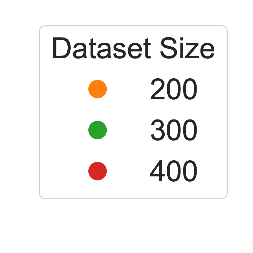
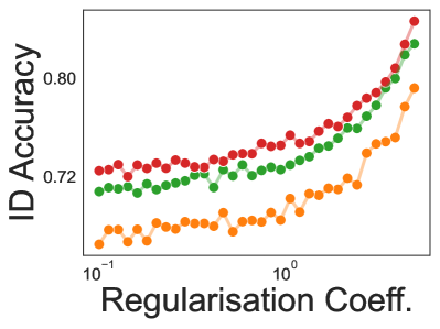
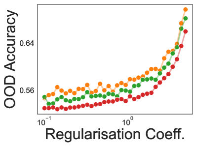
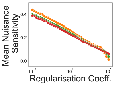
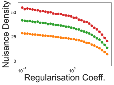
Noisy

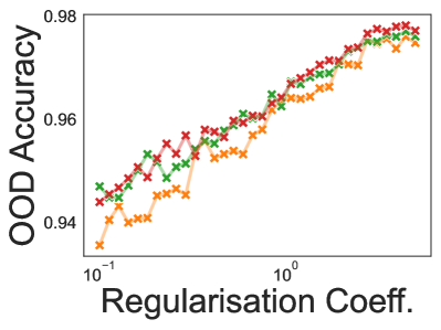
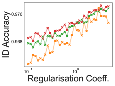
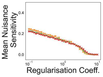
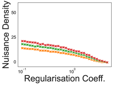
Noiseless

Figure 9: We show varying the strength of regularisation impacts the ID and OOD accuracy as well as the spurious sensitivity and density. While both ID and OOD accuracy increases with increasing regularisation coefficient, larger datasets have a noticeably smaller OOD accuracy in the noisy setting for all regularisation strengths. In all other settings, larger datasets have a higher accuracy and this is the main factor leading to the Accuracy-on-the-wrong-line behaviour. Regarding spurious sensitivity and density, for sufficiently large regularisation both the spurious sensitivity and the density drops to zero much faster for the noiseless setting than the noisy setting.

B.3 Colored MNIST dataset

As discussed in the main text, this dataset is derived from MNIST by introducing a color-based spurious correlation. Specifically, digits are initially assigned a binary label based on their numeric value (less than 5 or not), and this label is then corrupted with label noise probability $\eta$. To make this set of experiment more realistic, we use an algorithm that is supposed to be robust to distribution shift. In particular, we construct domains one with $0.35$ and one with $0.7$ fraction of the samples with correlated label and colour. Then, we optimise an average of the losses on these two domains. For test set, the spurious correlation is at $0.1$.

A three-layer MLP is then trained on this dataset to achieve zero training error by running the Adam optimizer for 1000 steps with $\ell_{2}$ regularization. The width of the MLP is varied from $16$ to $2048$ to generate various runs. The learning rate is set at 0.001. The accuracy on the training distribution is referred to as the ID accuracy, and the accuracy on the test distribution is referred to as the OOD accuracy. Each set of runs (multiple seeds etc) was run on a single GPU and took less than 30 minutes for the whole set.

B.4 Functional Map of the World (fMoW) Dataset

The original FMoW dataset [9] contains satellite images from various parts of the world, classified into five geographical regions: Africa, Asia, America, Europe, and Oceania, and labeled according to one of 30 objects in the image. It also includes additional metadata regarding the time the image was captured. The FMoW-CS dataset is constructed by introducing a correlation between the domain and the label, i.e. only sampling certain labels for certain domains. We use the domain-label pairing originally used by Shi et al. [35], which ensures that if the dataset is sampled according to this pairing, the population of each class relative to the total number of examples remains stable. In this work, we use a spurious correlation level of 0.9, meaning 90% of the training dataset follows the domain-label pairing, while the remaining 10% does not match any domain-label pairs. The domain-label pairing for FMoW-CS is detailed in Table 1. To simplify the problem further, we only select five labels instead of all thirty, which is the first in each of the rows.

Similar to our previous experiments, we also introduce label noise with a probability of 0.5. For the OOD test data, we use the original WILDS [17, 30] test set for FMoW, which essentially creates a distribution shift by thresholding based on a timestamp; images before that timestamp are ID and images after are OOD. To obtain various training runs, we fine-tuned ImageNet pre-trained models, including ResNet-18, ResNet-34, ResNet-50, ResNet-101, and DenseNet121, with various learning rates and weight decays on the FMoW-CS dataset. We also varied the width of the convolution layers to increase the width of each network. In total, we trained nearly 400 models using various configurations where each model was trained on a single 48GB NVIDIA Quadro RTX 6000 with 36 CPUs or a 32GB NVIDIA V100 with 28 CPUs. Each run took between 9 hours and 15 hours depending on problem parameters.

Noisy no Spurious correlation

Figure 10: Experiments on the FMoW dataset without spurious correlation shows almost zero correlation between ID and OOD accuracy.

Table 1: Domain-label pairing for FMoW-CS.

Domain (region)	Label
Asia	Military facility, multi-unit residential, tunnel opening, wind farm, toll booth, road bridge, oil or gas facility, helipad, nuclear powerplant, police station, port
Europe	Smokestack, barn, waste disposal, hospital, water treatment facility, amusement park, fire station, fountain, construction site, shipyard, solar farm, space facility
Africa	Place of worship, crop field, dam, tower, runway, airport, electric substation, flooded road, border checkpoint, prison, archaeological site, factory or powerplant, impoverished settlement, lake or pond
Americas	Recreational facility, swimming pool, educational institution, stadium, golf course, office building, interchange, car dealership, railway bridge, storage tank, surface mine, zoo
Oceania	Single-unit residential, parking lot or garage, race track, park, ground transportation station, shopping mall, airport terminal, airport hangar, lighthouse, gas station, aquaculture, burial site, debris or rubble

References

- Abe et al. [2022] Taiga Abe, Estefany Kelly Buchanan, Geoff Pleiss, Richard Zemel, and John P Cunningham. Deep ensembles work, but are they necessary? In Conference on Neural Information Processing Systems (NeurIPS), 2022.
- Aerni et al. [2023] Michael Aerni, Marco Milanta, Konstantin Donhauser, and Fanny Yang. Strong inductive biases provably prevent harmless interpolation. In International Conference on Learning Representations (ICLR), 2023.
- Arjovsky et al. [2019] Martin Arjovsky, Léon Bottou, Ishaan Gulrajani, and David Lopez-Paz. Invariant risk minimization. arXiv:1907.02893, 2019.
- Baek et al. [2022] Christina Baek, Yiding Jiang, Aditi Raghunathan, and J. Zico Kolter. Agreement-on-the-line: Predicting the performance of neural networks under distribution shift. In Conference on Neural Information Processing Systems (NeurIPS), 2022.
- Bartlett et al. [2020] Peter L Bartlett, Philip M Long, Gábor Lugosi, and Alexander Tsigler. Benign overfitting in linear regression. Proceedings of the National Academy of Sciences, 2020.
- Belkin et al. [2019] Mikhail Belkin, Daniel Hsu, Siyuan Ma, and Soumik Mandal. Reconciling modern machine-learning practice and the classical bias–variance trade-off. Proceedings of the National Academy of Sciences, 2019.
- Ben-Dov et al. [2024] Omri Ben-Dov, Jake Fawkes, Samira Samadi, and Amartya Sanyal. The role of learning algorithms in collective action. 2024.
- Brown et al. [2023] Bradley CA Brown, Anthony L Caterini, Brendan Leigh Ross, Jesse C Cresswell, and Gabriel Loaiza-Ganem. Verifying the union of manifolds hypothesis for image data. International Conference on Learning Representations (ICLR), 2023.
- Christie et al. [2018] Gordon Christie, Neil Fendley, James Wilson, and Ryan Mukherjee. Functional map of the world. In IEEE Conference on Computer Vision and Pattern Recognition (CVPR), 2018.
- Deng [2012] Li Deng. The mnist database of handwritten digit images for machine learning research. IEEE Signal Processing Magazine, 2012.
- Eastwood et al. [2024] Cian Eastwood, Shashank Singh, Andrei L Nicolicioiu, Marin Vlastelica Pogančić, Julius von Kügelgen, and Bernhard Schölkopf. Spuriosity didn’t kill the classifier: Using invariant predictions to harness spurious features. Conference on Neural Information Processing Systems (NeurIPS), 2024.
- Frenay and Verleysen [2014] Benoit Frenay and Michel Verleysen. Classification in the presence of label noise: A survey. IEEE Transactions on Neural Networks and Learning Systems, 2014.
- Goel et al. [2024] Shashwat Goel, Ameya Prabhu, Philip Torr, Ponnurangam Kumaraguru, and Amartya Sanyal. Corrective machine unlearning. arXiv:2402.14015, 2024.
- Hestness et al. [2017] Joel Hestness, Sharan Narang, Newsha Ardalani, Gregory Diamos, Heewoo Jun, Hassan Kianinejad, Md Mostofa Ali Patwary, Yang Yang, and Yanqi Zhou. Deep learning scaling is predictable, empirically. arXiv:1712.00409, 2017.
- Kaplan et al. [2020] Jared Kaplan, Sam McCandlish, Tom Henighan, Tom B Brown, Benjamin Chess, Rewon Child, Scott Gray, Alec Radford, Jeffrey Wu, and Dario Amodei. Scaling laws for neural language models. arXiv:2001.08361, 2020.
- Kim et al. [2023] Eungyeup Kim, Mingjie Sun, Aditi Raghunathan, and Zico Kolter. Reliable test-time adaptation via agreement-on-the-line. arXiv:2310.04941, 2023.
- Koh et al. [2021] Pang Wei Koh, Shiori Sagawa, Henrik Marklund, Sang Michael Xie, Marvin Zhang, Akshay Balsubramani, Weihua Hu, Michihiro Yasunaga, Richard Lanas Phillips, Irena Gao, Tony Lee, Etienne David, Ian Stavness, Wei Guo, Berton A. Earnshaw, Imran S. Haque, Sara Beery, Jure Leskovec, Anshul Kundaje, Emma Pierson, Sergey Levine, Chelsea Finn, and Percy Liang. WILDS: A benchmark of in-the-wild distribution shifts. In International Conference on Machine Learning (ICML), 2021.
- Kumar et al. [2022] Ananya Kumar, Aditi Raghunathan, Robbie Jones, Tengyu Ma, and Percy Liang. Fine-tuning can distort pretrained features and underperform out-of-distribution. arXiv:2202.10054, 2022.
- Lee et al. [2023] Donghwan Lee, Behrad Moniri, Xinmeng Huang, Edgar Dobriban, and Hamed Hassani. Demystifying disagreement-on-the-line in high dimensions. In International Conference on Machine Learning (ICML), 2023.
- Liang et al. [2023] Weixin Liang, Yining Mao, Yongchan Kwon, Xinyu Yang, and James Zou. Accuracy on the curve: On the nonlinear correlation of ML performance between data subpopulations. In International Conference on Machine Learning (ICML), 2023.
- Madry et al. [2018] Aleksander Madry, Aleksandar Makelov, Ludwig Schmidt, Dimitris Tsipras, and Adrian Vladu. Towards deep learning models resistant to adversarial attacks. In International Conference on Learning Representations (ICLR), 2018.
- Miller et al. [2021] John P Miller, Rohan Taori, Aditi Raghunathan, Shiori Sagawa, Pang Wei Koh, Vaishaal Shankar, Percy Liang, Yair Carmon, and Ludwig Schmidt. Accuracy on the line: on the strong correlation between out-of-distribution and in-distribution generalization. In International Conference on Machine Learning (ICML), 2021.
- Miller [1981] Kenneth S. Miller. On the inverse of the sum of matrices. Mathematics Magazine, 1981.
- Nakkiran et al. [2021] Preetum Nakkiran, Gal Kaplun, Yamini Bansal, Tristan Yang, Boaz Barak, and Ilya Sutskever. Deep double descent: Where bigger models and more data hurt. Journal of Statistical Mechanics: Theory and Experiment, 2021.
- Northcutt et al. [2021] Curtis Northcutt, Anish Athalye, and Jonas Mueller. Confident learning: Estimating uncertainty in dataset labels. In Journal of Artifical Intelligence Research (JAIR), 2021.
- Paleka and Sanyal [2023] Daniel Paleka and Amartya Sanyal. A law of adversarial risk, interpolation, and label noise. In International Conference on Learning Representations (ICLR), 2023.
- Parascandolo et al. [2021] Giambattista Parascandolo, Alexander Neitz, ANTONIO ORVIETO, Luigi Gresele, and Bernhard Schölkopf. Learning explanations that are hard to vary. In International Conference on Learning Representations (ICLR), 2021.
- Pope et al. [2021] Phillip Pope, Chen Zhu, Ahmed Abdelkader, Micah Goldblum, and Tom Goldstein. The intrinsic dimension of images and its impact on learning. International Conference on Learning Representations (ICLR), 2021.
- Qiu et al. [2023] GuanWen Qiu, Da Kuang, and Surbhi Goel. Complexity matters: Dynamics of feature learning in the presence of spurious correlations. In NeurIPS Workshop on Mathematics of Modern Machine Learning, 2023.
- Sagawa et al. [2022] Shiori Sagawa, Pang Wei Koh, Tony Lee, Irena Gao, Sang Michael Xie, Kendrick Shen, Ananya Kumar, Weihua Hu, Michihiro Yasunaga, Henrik Marklund, Sara Beery, Etienne David, Ian Stavness, Wei Guo, Jure Leskovec, Kate Saenko, Tatsunori Hashimoto, Sergey Levine, Chelsea Finn, and Percy Liang. Extending the wilds benchmark for unsupervised adaptation. In International Conference on Learning Representations (ICLR), 2022.
- Sanyal et al. [2020] Amartya Sanyal, Philip H. Torr, and Puneet K. Dokania. Stable rank normalization for improved generalization in neural networks and gans. In International Conference on Learning Representations (ICLR), 2020.
- Sanyal et al. [2021] Amartya Sanyal, Puneet K. Dokania, Varun Kanade, and Philip Torr. How benign is benign overfitting ? In International Conference on Learning Representations (ICLR), 2021.
- Schölkopf [2019] Bernhard Schölkopf. Causality for machine learning. 2019. doi: 10.1145/3501714.3501755.
- Shah et al. [2020] Harshay Shah, Kaustav Tamuly, Aditi Raghunathan, Prateek Jain, and Praneeth Netrapalli. The pitfalls of simplicity bias in neural networks. Conference on Neural Information Processing Systems (NeurIPS), 2020.
- Shi et al. [2023] Yuge Shi, Imant Daunhawer, Julia E Vogt, Philip Torr, and Amartya Sanyal. How robust is unsupervised representation learning to distribution shift? In The Eleventh International Conference on Learning Representations, 2023.
- Singla and Feizi [2021] Sahil Singla and Soheil Feizi. Salient imagenet: How to discover spurious features in deep learning? In International Conference on Learning Representations (ICLR), 2021.
- Sinha et al. [2018] Aman Sinha, Hongseok Namkoong, and John Duchi. Certifiable distributional robustness with principled adversarial training. In International Conference on Learning Representations (ICLR), 2018.
- Tanno et al. [2022] Ryutaro Tanno, Melanie F. Pradier, Aditya Nori, and Yingzhen Li. Repairing neural networks by leaving the right past behind. In Conference on Neural Information Processing Systems (NeurIPS), 2022.
- Teney et al. [2023] Damien Teney, Yong Lin, Seong Joon Oh, and Ehsan Abbasnejad. Id and ood performance are sometimes inversely correlated on real-world datasets. In Conference on Neural Information Processing Systems (NeurIPS), 2023.
- Tripuraneni et al. [2021a] Nilesh Tripuraneni, Ben Adlam, and Jeffrey Pennington. Overparameterization improves robustness to covariate shift in high dimensions. In Conference on Neural Information Processing Systems (NeurIPS), 2021a.
- Tripuraneni et al. [2021b] Nilesh Tripuraneni, Ben Adlam, and Jeffrey Pennington. Covariate shift in high-dimensional random feature regression. arXiv:2111.08234, 2021b.
- Vershynin [2018] Roman Vershynin. High-Dimensional Probability: An Introduction with Applications in Data Science. 2018.
- Wang et al. [2021] Jialu Wang, Yang Liu, and Caleb Levy. Fair classification with group-dependent label noise. In ACM conference on fairness, accountability, and transparency (FaccT), 2021.
- Wenzel et al. [2022] Florian Wenzel, Andrea Dittadi, Peter Gehler, Carl-Johann Simon-Gabriel, Max Horn, Dominik Zietlow, David Kernert, Chris Russell, Thomas Brox, Bernt Schiele, Bernhard Schölkopf, and Francesco Locatello. Assaying out-of-distribution generalization in transfer learning. In Conference on Neural Information Processing Systems (NeurIPS), 2022.
- Wu et al. [2022] Songhua Wu, Mingming Gong, Bo Han, Yang Liu, and Tongliang Liu. Fair classification with instance-dependent label noise. In Conference on Causal Learning and Reasoning (CLeaR), 2022.
- Zhang et al. [2017] Chiyuan Zhang, Samy Bengio, Moritz Hardt, Benjamin Recht, and Oriol Vinyals. Understanding deep learning requires rethinking generalization. In International Conference on Learning Representations (ICLR), 2017.
- Zhang et al. [2018] Hongyi Zhang, Moustapha Cisse, Yann N. Dauphin, and David Lopez-Paz. mixup: Beyond empirical risk minimization. In International Conference on Learning Representations (ICLR), 2018.