Text-Guided Alternative Image Clustering
Abstract
Traditional image clustering techniques only find a single grouping within visual data. In particular, they do not provide a possibility to explicitly define multiple types of clustering. This work explores the potential of large vision-language models to facilitate alternative image clustering. We propose Text-Guided Alternative Image Consensus Clustering (TGAICC), a novel approach that leverages user-specified interests via prompts to guide the discovery of diverse clusterings. To achieve this, it generates a clustering for each prompt, groups them using hierarchical clustering, and then aggregates them using consensus clustering. TGAICC outperforms image- and text-based baselines on four alternative image clustering benchmark datasets. Furthermore, using count-based word statistics, we are able to obtain text-based explanations of the alternative clusterings. In conclusion, our research illustrates how contemporary large vision-language models can transform explanatory data analysis, enabling the generation of insightful, customizable, and diverse image clusterings. 111Code available at https://github.com/AndSt/alternative_image_clustering.
1 Introduction
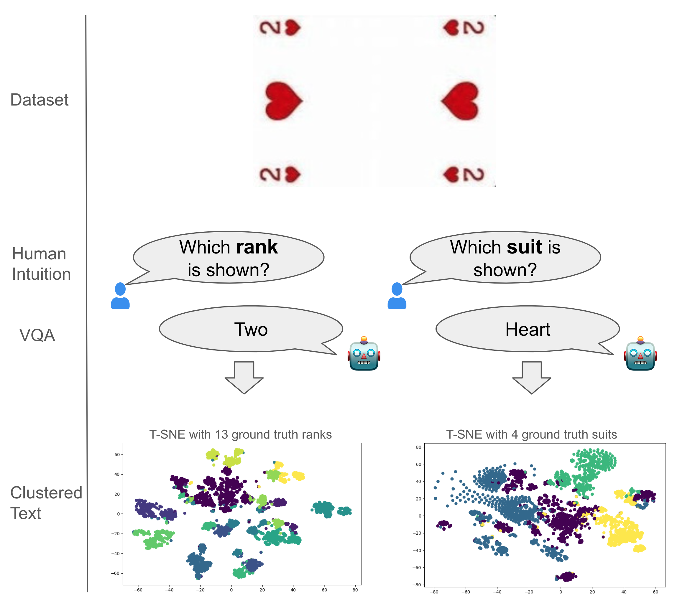
Exploratory data analysis (EDA) serves a crucial function in the comprehension and analysis of data Tukey (1970). Clustering arises as a cornerstone EDA methodology, facilitating the grouping of similar data points into coherent groups. A dataset of images, for example, can be clustered based on semantic similarities between the shown objects. Nevertheless, within applied contexts, variations in user requirements or foci demand distinct clustering formations. One might, for instance, cluster a dataset of cards by rank or by suit (see Figure 1). In such circumstances, it is advantageous to derive multifaceted insights into a dataset from diverse perspectives.
Current approaches in alternative image clustering either rely on image-based features Mautz et al. (2018); Miklautz et al. (2020) or utilize text through image-text bi-encoders, often with architectures resembling CLIP Radford et al. (2021); Yao et al. (2024). These methods, while powerful, neglect the rich insights that can be extracted by models explicitly trained to retrieve specific aspects of information from images using text (e.g., visual question answering (VQA) models Antol et al. (2015)). Stephan et al. (2024) demonstrate the effectiveness of using generated text descriptions to improve standard image clustering tasks, i.e. in scenarios where a single clustering structure is expected.
We aim to use image-to-text models to obtain alternative clusterings. By encoding visual content into text, similarity dimensions beyond the visual features can be explored, potentially uncovering interpretable relationships. We introduce TGAICC (Text-Guided Alternative Image Consensus Clustering), a clustering method that uses the generations of multiple image-to-text models to obtain alternative clusterings. TGAICC incorporates VQA models to generate multiple textual descriptions of images and then clusters the images based on the generated natural language descriptions. We identify similar clusterings using their mutual information, group them using hierarchical clustering and aggregate them using consensus clustering to form refined, alternative clusterings.
Our experimental setup employs four widely used alternative image clustering datasets, each possessing two or three ground truth labelings (e.g., playing cards clustered by rank or suit). We compare TGAICC against baselines for alternative clustering using image-only features and baselines that make use of the generated text. Our experiments demonstrate the following key findings: methods clustering the generated text outperform methods based on image features on these alternative clustering datasets, underscoring the power of textual representations in capturing diverse aspects of similarity. Further, TGAICC, on average, achieves superior results across the evaluated datasets and metrics when compared to all other methods, highlighting the effectiveness of our framework in leveraging image-to-text models to uncover alternative and insightful clusterings. Lastly, we can better interpret the clusterings by explaining the content using word statistics. Our case study on the cards dataset shows that text provides an opportunity to obtain an informative overview of the data.
In summary, our research provides the following contributions:
-
1.
We introduce a prompt-based setup to obtain alternative image clusterings.
-
2.
We introduce TGAICC, a method that combines ideas from multi-modality, hierarchical clustering, and consensus clustering to obtain alternative clusterings.
-
3.
Our experiments on four common alternative image clustering datasets show that our TGAICC outperforms our baselines
-
4.
Our methodology enables the ability to generate textual cluster explanations, offering a clear overview of the unique content captured within each alternative clustering.
2 Related Work
This work builds upon image clustering, consensus clustering, and alternative clustering approaches. We provide a brief overview of these relevant areas and describe the necessary background.
2.1 Image Clustering
Research in image clustering has addressed several standard issues, and a variety of techniques have been developed to tackle them. (Ezugwu et al., 2022) provide a survey on clustering approaches. Classic approaches like k-means Lloyd (1982) have demonstrated effectiveness but often struggle with complex or high-dimensional image data. To address these limitations, more recent work has explored deep clustering methods such as DEC Xie et al. (2016) and IDEC Guo et al. (2017). In addition to these core techniques, representation learning and more specifically, self-supervised learning Jaiswal et al. (2021) has emerged as a vital aspect of image clustering Lehner et al. (2023); Adaloglou et al. (2023). In Contrastive Clustering Li et al. (2021), the authors use one loss contrasting image features and another loss contrasting clustering features, i.e., the predicted cluster of two augmentations of the same image. A different approach is used in Text-Guided Image Clustering Stephan et al. (2024). This paradigm leverages image-to-text models and subsequently cluster text. The observation that text often outperforms image-based features motivates this work.
2.2 Consensus Clustering
Variability in clustering results arises from different clustering algorithms or variations in their initializations. Given that different clusterings potentially reveal different insights (e.g., accurately identifying a cluster representing "hearts"). Consensus clustering methods aim to aggregate results from multiple base clustering algorithms to produce a more robust and stable final clustering. The problem was formalized by (Strehl and Ghosh, 2002) and the authors introduce the Cluster-based Similarity Partitioning Algorithm (CSPA), HyperGraph Partitioning Algorithm (HGPA), and the Meta-CLustering Algorithm (MCLA). All three employ clustering similarity functions, e.g. Normalized Mutual Information (NMI), to construct a similarity graph and use graph theory to obtain a consensus clustering. In (Li and Ding, ), non-negative matrix factorization (NMF) is used to obtain a consensus clustering. The Hybrid Bipartite Graph Formulation (HBGF) Fern and Brodley (2004) employs a bipartite graph representation. In (Miklautz et al., 2022), the authors introduce DECCS, a deep learning-based consensus method, which learns a representation on which heterogeneous clustering algorithms share a consensus on the obtained clusterings.
2.3 Alternative Clustering
Clustering methods usually focus on finding a single optimal clustering solution. Motivated by the fact that there may be multiple meaningful ways to group data points, alternative clustering approaches aim to uncover multiple, diverse clustering structures within the same data Yu et al. (2024); Müller et al. (2012).
Cui et al. (2007) first apply a traditional clustering algorithm and then transform the dataset into a feature space orthogonal to the current clustering. Two strategies are proposed: orthogonal clustering (orth1) and clustering in orthogonal subspaces (orth2). In contrast, Non-redundant K-means (Nr-Kmeans) Mautz et al. (2018) simultaneously identifies multiple clusterings within a dataset by iteratively rotating the feature space and assigning features to specific clusterings. ENRC Miklautz et al. (2020) is a deep non-redundant clustering method that learns multiple clusterings from a dataset by (soft-)assigning each dimension of the embeddings space to a clustering. In (Kwon et al., 2024), the authors provide initial text criteria, e.g., suits and ranks, and use image-to-text models to extract information, and then GPT-4 to obtain cluster names and classify images into clusters. Thus, this approach is expensive. In concurrent work, (Yao et al., 2024) use GPT-4 to generate cluster name candidates and contrastively fine-tune CLIP Radford et al. (2021).
2.4 Image-To-Text Models
Recently, the development of multimodal models has seen rapid advancement. Image-to-text models, in particular, learn to associate visual content with corresponding textual descriptions, which is useful for, e.g., visual question-answering (VQA) Yin et al. (2023); Antol et al. (2015).
Flamingo Alayrac et al. (2022) allows interleaving images and text by using Perceiver Resamplers on top of pre-trained models. BLIP and BLIP2 Li et al. (2022, 2023a) employ a frozen image encoder along with a frozen LLM to generate text. LLaVA and LLaVA-NeXTLiu et al. (2023b, a) convert image patches into token embeddings using a fixed Vision Transformer encoder followed by a trained MLP. These tokens then become the input for the LLM, enhancing the descriptive results.
In this work, we use LLaVA to extract relevant information from images. More specifically, we frame the image-to-text generation as a VQA task: we prompt LLaVA with an image and corresponding questions about it to generate natural language descriptions of the image.
3 TGAICC
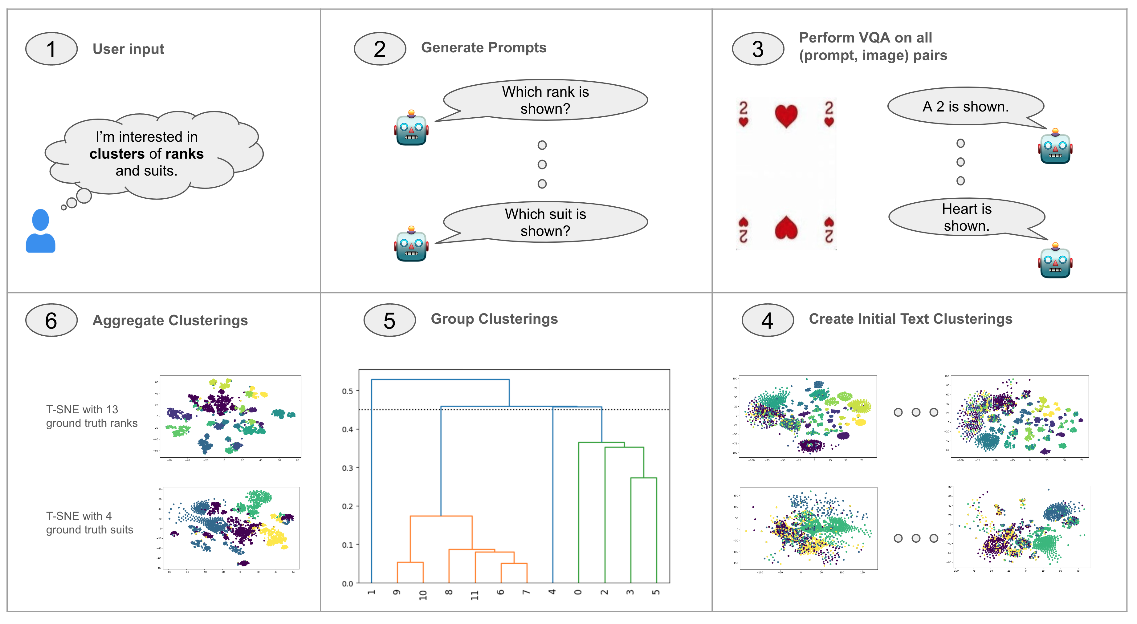
We use image-to-text models, specifically models that are able to describe specific aspects of information from images in order to obtain different clusterings. Thus, we design prompts to perform VQA. It is well known Bach et al. (2022); Sclar et al. (2024) that responses to seemingly semantically equal prompts might vary heavily. Thus, we use multiple formulations of each prompt and aggregate their clusterings afterward. Figure 2 gives an overview of the process.
Setup. The input to TGAICC is a dataset of datapoints, initial prompts, and, as common in the alternative-clustering literature, the number of clusters in the ground truth clusterings . E.g., means the algorithm should return one clustering with and one clustering with clusters. Note that the difference to the traditional alternative clustering setup is that we give additional initial prompts. The output is comprised of clusterings where the data points are grouped into clusters.
3.1 Initialization
The following two paragraphs describe the steps 1-4 in Figure 2.
Prompt Design We write a query and ask GPT-4 OpenAI et al. (2024) to automatically generate additional questions. The specific prompt is ’Generate three diverse paraphrases for the following question: {initial question}’. Further, we generate a variation of each prompt by appending the directive "Write concisely.", aiming to reduce the verbosity of the responses. This is based on the observation that image clusters are often described by succinct short descriptors, e.g., the datasets in our experiments or ImageNet-based Deng et al. (2009) clustering datasets. Thus, these prompts align with our knowledge about the clustering tasks.
Initial Clustering First, we perform VQA for each pair of images and prompts, generating responses relevant to the visual content. Next, we create text representations using both traditional TF-IDF Sparck Jones (1988) and an advanced sentence embedding model, namely gte-large Li et al. (2023b). Finally, we apply k-means to these text representations and obtain a clustering for each prompt and each representation.
3.2 Grouping
The input to the grouping stage are pairs of prompt and corresponding clustering and the number of ground truth clustering sizes , e.g. . The goal is to obtain groups of clusterings to later find consensus between the individual clusterings explaining the data from a similar perspective. This is displayed in step 5 of Figure 2. Specifically, we aim to connect semantically similar clusterings and detect potential outlier clusterings, which are caused by prompts leading to unexpected or inconsistent VQA outcomes and are not useful for our final clustering. Find examples of generated text in Table 6.
Therefore, we compute the similarity of two clusterings using Adjusted Mutual Information (AMI) Vinh et al. (2010). We choose AMI as it is a standard clustering metric based on information theory. Then, we use a spanning-tree-based hierarchical clustering Müllner (2011) algorithm222Algorithm is readily available in the Scipy library Virtanen et al. (2020): https://docs.scipy.org/doc/scipy/reference/generated/scipy.cluster.hierarchy.fcluster.html to systematically group similar prompts, facilitating a structured analysis of clustering behavior (see step 5 of Figure 2). The basic idea is that for a threshold , two clusterings are connected if their distance is less than , i.e. . Here, we use two strategies, which we call “min” and “max”. For “min”, we find a minimum threshold such that the resulting number of groups is equal to the number of expected groupings . For “max”, we find a maximum threshold such that this constraint is fulfilled. We use the trivial solution to iterate over all thresholds in in steps of as the runtime is negligible.
3.3 Aggregation
In the end, we synthesize each group of clusterings. Given that we aggregate potentially very different clusterings, it is beneficial to use different aggregation schemes. Therefore, we apply multiple consensus clustering algorithms for each group and choose the instance with the lowest clustering loss. Specifically, we employ MCLA, HBGF, CSPA, and NMF (Strehl and Ghosh, 2002; Li and Ding, ) to aggregate the clusterings within the groups333We used the library Cluster Ensembles: https://github.com/GGiecold-zz/Cluster_Ensembles. Thereby, we aim to use consensus clustering to combine the strength of multiple clusterings. In our ablation analysis we also test the simple solution where we concatenate the generated text of the prompts in each clustering group and perform k-means on the concatenated string.
4 Experiments
In this section, we introduce the experimental setup. Afterwards, we discuss the main results obtained, highlighting the performance of TGAICC and text-based methods. Additionally, we provide an ablation study, systematically analyzing the impact of various components and prompts on the overall performance. Finally, we perform a simple cluster explainability method to get a textual overview of the data.
| Dataset | #samples | #clusters | Size |
|---|---|---|---|
| Fruits-360 | 4856 | 4; 4 | 100x100 |
| Cards | 8029 | 3; 4 | 224x224 |
| GTSRB | 6720 | 4; 2 | 15x15 to 250x250 |
| NR-Objects | 10000 | 6; 2; 3 | 100x100 |
4.1 Experimental Setup
In this section, we outline the key components of our experimental setup, including the evaluation metrics, data representations, and models used. All experiments were run on a single A100 GPU. VQA took approximately 24 hours and TGAICC experiments took about the same time. Embedding text and running consensus clustering are the most time consuming elements. Each algorithm is executed 10 times with different random states, and we report the average performance across these runs.
| Image | TF-IDF | SBERT | TGAICC | |||||||||
| Dataset | Type | k-means | orth-1 | orth-2 | Nr-Kmeans | ENRC | Avg. Prompt | Concatenate | Avg. Prompt | Concatenate | ||
| Fruits-360 | fruit | ARI | 27.40 | 31.50 | 30.80 | 35.40 | 26.00 | 14.80 | 20.10 | 15.10 | 17.20 | 18.60 |
| AMI | 41.30 | 42.10 | 42.90 | 50.60 | 36.70 | 24.80 | 32.20 | 25.00 | 28.60 | 26.90 | ||
| colour | ARI | 33.20 | 35.40 | 33.50 | 40.90 | 39.70 | 40.00 | 54.60 | 47.40 | 51.60 | 54.70 | |
| AMI | 47.30 | 53.30 | 51.70 | 55.50 | 54.90 | 50.70 | 65.50 | 56.90 | 60.80 | 64.80 | ||
| GTSRB | type | ARI | 41.70 | 46.80 | 46.80 | 22.70 | 38.20 | 45.10 | 61.00 | 49.70 | 57.50 | 58.00 |
| AMI | 51.50 | 55.50 | 55.50 | 38.60 | 72.50 | 52.40 | 67.90 | 55.50 | 63.20 | 64.60 | ||
| colour | ARI | 23.00 | 0.10 | 0.10 | 49.00 | 55.90 | 79.20 | 87.40 | 88.50 | 90.00 | 88.00 | |
| AMI | 33.40 | 0.10 | 0.10 | 43.30 | 28.30 | 73.70 | 82.30 | 82.70 | 84.50 | 83.00 | ||
| Cards | rank | ARI | 30.10 | 29.70 | 26.70 | 35.70 | 33.10 | 24.30 | 24.70 | 33.00 | 50.70 | 34.70 |
| AMI | 47.80 | 47.60 | 41.70 | 55.20 | 52.40 | 41.30 | 41.60 | 50.00 | 68.40 | 50.20 | ||
| suit | ARI | 25.90 | 1.10 | 3.80 | 10.60 | 14.30 | 19.70 | 29.60 | 25.90 | 28.30 | 29.70 | |
| AMI | 34.40 | 1.20 | 8.20 | 16.60 | 19.80 | 27.40 | 37.10 | 33.60 | 35.40 | 38.30 | ||
| NR-Objects | shape | ARI | 95.30 | 94.40 | 94.40 | 76.00 | 72.70 | 65.70 | 94.50 | 75.90 | 95.00 | 100.00 |
| AMI | 96.20 | 95.10 | 95.10 | 82.20 | 82.70 | 71.30 | 96.50 | 79.40 | 95.80 | 100.00 | ||
| material | ARI | 0.00 | 26.70 | 30.60 | 30.70 | 31.60 | 9.20 | 1.60 | 14.80 | 0.00 | 9.00 | |
| AMI | 0.00 | 25.90 | 38.80 | 32.70 | 39.40 | 10.10 | 1.80 | 15.00 | 0.00 | 17.10 | ||
| colour | ARI | 9.70 | 87.00 | 75.10 | 50.40 | 45.70 | 66.80 | 91.10 | 81.20 | 83.70 | 97.80 | |
| AMI | 21.70 | 93.00 | 79.00 | 65.70 | 66.00 | 81.20 | 95.30 | 88.30 | 91.40 | 97.90 | ||
| Avg. | ARI | 31.81 | 39.19 | 37.98 | 39.04 | 39.69 | 40.53 | 51.62 | 47.94 | 52.67 | 54.50 | |
| AMI | 41.51 | 45.98 | 45.89 | 48.93 | 50.30 | 48.10 | 57.80 | 54.04 | 58.68 | 60.31 | ||
4.1.1 Metrics
We employ two widely used metrics to assess the performance of our clustering models. The Adjusted Rand Index (ARI) Rand (1971) measures the similarity between the predicted cluster assignments and the ground truth labels, adjusting for chance agreement. The Adjusted Mutual Information (AMI) Vinh et al. (2010) quantifies the shared information between the predicted clusters and the true labels. We multiply by 100 to increase readability.
4.1.2 Representations
We utilize image- and text-based representations to capture different aspects of the data.
Image Embeddings: We utilize the LLaVA-NeXT model Liu et al. (2023a), which incorporates the image encoder of a frozen CLIP model. This allows us to directly use the image embeddings learned during the contrastive pre-training of CLIP Radford et al. (2021) for our clustering tasks.
Statistical text embeddings: We employ Term Frequency-Inverse Document Frequency (TF-IDF) embeddings, a standard word frequency-based technique for representing documents.
Neural text embeddings: To better capture semantic relationships, we employ the “gte-large”444Model is available on Hugging Face (https://huggingface.co/thenlper/gte-large, and is used via the Sentence-BERT (SBERT) library Reimers and Gurevych (2019) model Li et al. (2023b), a state-of-the-art sentence encoder.
4.1.3 Datasets
In the following, we briefly describe the used datasets. Table 1 summarizes the relevant statistics for all datasets. More details about datasets and corresponding prompts are in Appendix B.
Cards Yao et al. (2023) This dataset is primarily used for classification tasks but contains attributes suitable for clustering based on card suit and rank.
Fruits-360 Mure\textcommabelowsan and Oltean (2018) The dataset is composed of images that can be clustered by fruit type (citrus, berries, etc.) and color.
NR-Objects Miklautz et al. (2020) The dataset contains images of objects (e.g., cubes), which can be clustered by shape, material, or color.
German Traffic Sign Recognition (GTSRB) Houben et al. (2013) This dataset contains traffic signs and can be clustered by color and traffic sign type.
4.1.4 Baselines
We use multiple image-based alternative clustering baselines and baselines using the generated text. The code is implemented using the ClustPy555https://github.com/collinleiber/ClustPy library Leiber et al. (2023). Additional details are given in Appendix C.
Orth Cui et al. (2007) iteratively identifies several clusterings by first clustering using PCA (keeping of the variance) in combination with k-means and then creating a new orthogonal feature space. There are two strategies for orthogonalization: orthogonal clustering (orth-1) and clustering in orthogonal subspaces (orth-2).
Nr-Kmeans Mautz et al. (2018) simultaneously optimizes several clusterings by assigning each clustering result a separate subspace in which k-means is executed.
ENRC Miklautz et al. (2020) is a deep clustering method that assigns multiple clusterings to a dataset by (soft-)assigning each dimension of the embeddings space to a clustering.
Avg. Prompt. We measure the performance of clustering each text generated per prompt and subsequentially report the average performance.
Concat. by Category. We manually group all prompts together that belong to the same clustering type (e.g., “rank” or “suit”), concatenate all generated text, and cluster it using k-means.
4.2 Main Experiments
The results of our main experiments are shown in Table 2. They reveal that, on average, text-based methods, including TGAICC, outperform image-based methods. Further, we observe that TGAICC, on average, demonstrates superiority over avg. prompting and concatenation baselines. In addition, we can see that clustering by material in the NR-Objects dataset does not work in the text domain.
| TF-IDF | SBERT | |||||||||
| selection | consensus | selection | consensus | |||||||
| min | max | min | max | min | max | min | max | |||
| Fruits-360 | fruit | ARI | 20.80 | 24.60 | 17.40 | 19.50 | 19.60 | 17.20 | 15.80 | 18.60 |
| AMI | 36.60 | 39.10 | 29.00 | 32.90 | 33.00 | 30.90 | 23.20 | 26.90 | ||
| colour | ARI | 51.80 | 52.20 | 51.10 | 51.90 | 58.60 | 57.20 | 54.30 | 54.70 | |
| AMI | 61.70 | 62.20 | 60.70 | 61.40 | 71.50 | 66.40 | 64.90 | 64.80 | ||
| GTSRB | type | ARI | 52.70 | 73.20 | 49.70 | 54.10 | 50.80 | 58.00 | 51.60 | 58.00 |
| AMI | 60.80 | 75.40 | 56.60 | 60.40 | 57.80 | 64.10 | 60.00 | 64.60 | ||
| colour | ARI | 74.70 | 74.00 | 87.10 | 87.30 | 73.10 | 70.20 | 88.90 | 88.00 | |
| AMI | 70.70 | 70.10 | 81.60 | 81.80 | 70.20 | 68.60 | 83.20 | 83.00 | ||
| Cards | rank | ARI | 28.60 | 28.00 | 27.00 | 26.90 | 40.30 | 56.00 | 36.30 | 34.70 |
| AMI | 48.30 | 47.00 | 47.60 | 46.20 | 58.50 | 72.20 | 51.30 | 50.20 | ||
| suit | ARI | 19.40 | 20.10 | 21.60 | 21.10 | 19.60 | 19.90 | 22.40 | 29.70 | |
| AMI | 29.30 | 28.90 | 23.60 | 23.70 | 30.50 | 27.30 | 27.40 | 38.30 | ||
| NR-Objects | shape | ARI | 98.70 | 98.90 | 99.30 | 99.30 | 100.00 | 100.00 | 100.00 | 100.00 |
| AMI | 97.60 | 97.90 | 98.90 | 98.70 | 100.00 | 100.00 | 100.00 | 100.00 | ||
| material | ARI | 23.10 | 22.40 | 0.10 | 1.00 | 0.00 | 0.00 | 9.00 | 9.00 | |
| AMI | 22.70 | 22.20 | 0.10 | 1.80 | 0.00 | 0.00 | 17.10 | 17.10 | ||
| colour | ARI | 33.30 | 33.30 | 80.00 | 84.10 | 43.60 | 43.60 | 97.80 | 97.80 | |
| AMI | 65.20 | 65.20 | 87.50 | 90.10 | 66.60 | 66.60 | 97.90 | 97.90 | ||
| Avg. | ARI | 44.79 | 47.41 | 48.14 | 49.47 | 45.07 | 46.90 | 52.90 | 54.50 | |
| AMI | 54.77 | 56.44 | 53.96 | 55.22 | 54.23 | 55.12 | 58.33 | 60.31 | ||
See Table 6 for VQA examples. The main takeaway is that, in many cases, the VQA model provides too much information, even information that should be used for a different clustering, e.g., color or shape. This highlights a core limitation of our methodology. If the text generation does not work sufficiently well, the subsequent clustering can not work.
| TF-IDF | SBERT | ||||
|---|---|---|---|---|---|
| Prompt | ARI | AMI | ARI | AMI | |
| suit | Can you tell me the suit of the playing card shown in the picture? | 25.42 | 31.25 | 25.42 | 31.25 |
| What suit does the playing card in the image belong to? | 25.59 | 33.53 | 25.59 | 33.53 | |
| Could you identify the suit of the playing card depicted in the photo? | 29.29 | 33.64 | 29.29 | 33.64 | |
| Can you tell me the suit of the playing card shown in the picture? Answer concisely. | 24.25 | 37.32 | 24.25 | 37.32 | |
| What suit does the playing card in the image belong to? Answer concisely. | 28.97 | 36.35 | 28.97 | 36.35 | |
| Could you identify the suit of the playing card depicted in the photo? Answer concisely. | 21.85 | 29.71 | 21.85 | 29.71 | |
| rank | Can you tell me the rank of the card shown in the picture? | 26.76 | 43.33 | 26.76 | 43.33 |
| What is the numerical or face value of the card displayed in the image? | 32.06 | 47.36 | 32.06 | 47.36 | |
| What level or position does the card in the photo hold? | 31.52 | 47.28 | 31.52 | 47.28 | |
| Can you tell me the rank of the card shown in the picture? Answer concisely. | 37.48 | 55.42 | 37.48 | 55.42 | |
| What is the numerical or face value of the card displayed in the image? Answer concisely. | 38.79 | 56.09 | 38.79 | 56.09 | |
| What level or position does the card in the photo hold? Answer concisely. | 31.15 | 50.44 | 31.15 | 50.44 | |
Nevertheless, TGAICC is model-agnostic and can be used with any VQA image-to-text system. In this way, it can make use of future advancements in VQA models.
4.3 Aggregation ablation
In this ablation study, we investigate the aggregation components of TGAICC. More specifically, we investigate the impact of the thresholding and aggregation strategies on clustering performance.
Setup. We ablate the “min” and “max” thresholding strategies, which find the minimum and maximum threshold such that the number of clustering groups corresponds to the expected number of alternative clusterings. We experiment with the consensus-clustering-based aggregation scheme used in TGAICC and compare it to the simple “concatenation” baseline, which concatenates the text of the corresponding clustering groups. Results are shown in Table 3. Note that TGAICC is consensus-max.
Results. Our analysis reveals that consensus clustering outperforms concatenation-based selection. Furthermore, SBERT-based clustering outperforms TF-IDF-based clustering. We observe that the performance of the ’min’ and the ’max’ strategy are very similar, which indicates the stability of the method w.r.t. the thresholding strategy.
4.4 Individual prompt analysis
TGAICC is based on the aggregation of multiple clusterings, which in turn are based on generated texts using different VQA prompts. As known from other tasks Sclar et al. (2024), different prompts potentially result in high-performance variance.
Setup. In Table 4 we analyze the clustering performance per prompt on the case study of the Cards dataset. Note that again we execute k-means 10 times and present the averaged results.
Results. In the case study, the addition of the prompt “Answer concisely” mostly yields similar clustering results, with a slight performance advantage when the “Answer concisely” prompt is included. Furthermore, we note a significant variation in clustering performance across different prompts.
4.5 Explainability
Our cluster explainability aims to provide insights into the different clustering possibilities. This understanding is essential for interpreting and validating clustering outcomes. We use a simple word frequency-based algorithm to explain the data.
| Suit | Rank | ||
| Truth | Top Words | Truth | Top Words |
| heart | heart | ace | ace |
| diamond | diamond | king | king |
| club | club | queen | queen |
| spade | spade | jack | jack |
| 5 | heart | ||
| 9 | spade | ||
| 3 | rank | ||
| 4 | club | ||
| 6 | diamond | ||
| 10 | 10 | ||
| 2 | twos | ||
| 8 | 8 | ||
| 7 | 7 | ||
| Material | Image | Question | Generated Text |
|---|---|---|---|
| Rubber |
![[Uncaptioned image]](/html/2406.18589/assets/figures/dataset_examples/CLEVR_train_000010.png)
|
What substance is the item in the picture made of? Answer concisely. | Plastic |
| What substance is the item in the picture made of? | The item in the picture appears to be a sphere made of a smooth, shiny material that could be plastic, metal, or a similar synthetic material. It’s difficult to determine the exact material without more information or a closer inspection. | ||
| Metal |
![[Uncaptioned image]](/html/2406.18589/assets/figures/dataset_examples/CLEVR_train_004915.png)
|
What substance is the item in the picture made of? Answer concisely. | The item in the picture is made of metal. |
| Can you identify the material used in the object shown in the image? Answer concisely. | The object in the image appears to be made of a shiny, reflective material, possibly metal or a metal-like material. | ||
| What is the composition of the object depicted in the photo? Answer concisely. | The object in the photo is a 3D rendering of a red cube. |
Setup. For a specific final clustering of TGAICC, we concatenate all generated texts belonging to the prompts used to obtain this clustering. The resulting text is changed to lowercase and made singular. Finally, to explain a final clusterings, we determine the most frequently occurring words, where is the number of clusters of the respective clustering. For instance for the suit clustering . Table 5 shows the resulting words for the Cards dataset. We reorder the ground truth cluster names suitably.
Analysis. Notably, the explainability method effectively identifies the “suits” cluster names, providing a comprehensive description of this clustering type, even though clustering performance has an AMI of less than 40%. Additionally, the frequency analysis exposed many of the card types in the dataset. However, suit names are also assigned as cluster names for the expected card ranking clusters (e.g., “heart” as the top word of the “10” cluster). Figure 6 presents concrete examples demonstrating that Visual Question Answering (VQA) models often provide additional information, such as suit, thereby explaining the inclusion of suits as rank names.
5 Discussion
5.1 Text-driven data interaction
Textual data, as a fundamental form of human communication, offers a natural and intuitive interface for interacting with complex datasets. Our method capitalizes on this inherent connection by utilizing textual prompts for VQA models to guide alternative clusterings. This approach aligns with real-world scenarios where users possess domain knowledge and seek answers to specific questions. We envision a future where users can explore datasets from diverse perspectives and test emerging hypotheses interactively, using text. Our research contributes to this scenario.
5.2 Domain Expertise
Our approach incorporates domain expertise, recognizing that users often either have specific questions or some knowledge about their data. This stands in contrast to the traditional clustering setup, which typically operates without user input. By leveraging domain knowledge, our approach aligns with real-world scenarios and allows for more targeted and insightful data exploration.
6 Conclusion
In conclusion, this research introduces TGAICC (Text-Guided Alternative Image Consensus Clustering), a novel approach that leverages prompting to inject domain knowledge and human intuition into the clustering process. The experiments on four common alternative image clustering benchmarks demonstrate that TGAICC outperforms competitive image- and text-based baselines. Furthermore, the inherent explainability of text enables a deeper understanding of the underlying data cluster formations.
By utilizing textual prompts, we can explicitly guide the clustering process from various angles simultaneously, aligning with human intuition. This approach offers a more comprehensive and flexible way to analyze visual data, revealing insights that might be missed by traditional clustering methods.
References
- Adaloglou et al. (2023) Nikolas Adaloglou, Felix Michels, Hamza Kalisch, and Markus Kollmann. 2023. Exploring the limits of deep image clustering using pretrained models. In 34th British Machine Vision Conference 2023, BMVC 2023, Aberdeen, UK, November 20-24, 2023. BMVA.
- Alayrac et al. (2022) Jean-Baptiste Alayrac, Jeff Donahue, Pauline Luc, Antoine Miech, Iain Barr, Yana Hasson, Karel Lenc, Arthur Mensch, Katherine Millican, Malcolm Reynolds, Roman Ring, Eliza Rutherford, Serkan Cabi, Tengda Han, Zhitao Gong, Sina Samangooei, Marianne Monteiro, Jacob L Menick, Sebastian Borgeaud, Andy Brock, Aida Nematzadeh, Sahand Sharifzadeh, Mikoł aj Bińkowski, Ricardo Barreira, Oriol Vinyals, Andrew Zisserman, and Karén Simonyan. 2022. Flamingo: a visual language model for few-shot learning. In Advances in Neural Information Processing Systems, volume 35, pages 23716–23736. Curran Associates, Inc.
- Antol et al. (2015) Stanislaw Antol, Aishwarya Agrawal, Jiasen Lu, Margaret Mitchell, Dhruv Batra, C. Lawrence Zitnick, and Devi Parikh. 2015. Vqa: Visual question answering. In Proceedings of the IEEE International Conference on Computer Vision (ICCV).
- Bach et al. (2022) Stephen H. Bach, Victor Sanh, Zheng-Xin Yong, Albert Webson, Colin Raffel, Nihal V. Nayak, Abheesht Sharma, Taewoon Kim, M Saiful Bari, Thibault Fevry, Zaid Alyafeai, Manan Dey, Andrea Santilli, Zhiqing Sun, Srulik Ben-David, Canwen Xu, Gunjan Chhablani, Han Wang, Jason Alan Fries, Maged S. Al-shaibani, Shanya Sharma, Urmish Thakker, Khalid Almubarak, Xiangru Tang, Xiangru Tang, Mike Tian-Jian Jiang, and Alexander M. Rush. 2022. Promptsource: An integrated development environment and repository for natural language prompts.
- Cui et al. (2007) Ying Cui, Xiaoli Z. Fern, and Jennifer G. Dy. 2007. Non-redundant multi-view clustering via orthogonalization. In Proceedings of the 7th IEEE International Conference on Data Mining (ICDM 2007), October 28-31, 2007, Omaha, Nebraska, USA, pages 133–142. IEEE Computer Society.
- Deng et al. (2009) Jia Deng, Wei Dong, Richard Socher, Li-Jia Li, Kai Li, and Li Fei-Fei. 2009. Imagenet: A large-scale hierarchical image database. In 2009 IEEE Conference on Computer Vision and Pattern Recognition, pages 248–255.
- Ezugwu et al. (2022) Absalom E. Ezugwu, Abiodun M. Ikotun, Olaide O. Oyelade, Laith Abualigah, Jeffery O. Agushaka, Christopher I. Eke, and Andronicus A. Akinyelu. 2022. A comprehensive survey of clustering algorithms: State-of-the-art machine learning applications, taxonomy, challenges, and future research prospects. Engineering Applications of Artificial Intelligence, 110:104743.
- Fern and Brodley (2004) Xiaoli Zhang Fern and Carla E. Brodley. 2004. Solving cluster ensemble problems by bipartite graph partitioning. In Proceedings of the Twenty-First International Conference on Machine Learning, ICML ’04, page 36, New York, NY, USA. Association for Computing Machinery.
- Guo et al. (2017) Xifeng Guo, Long Gao, Xinwang Liu, and Jianping Yin. 2017. Improved deep embedded clustering with local structure preservation. In Proceedings of the Twenty-Sixth International Joint Conference on Artificial Intelligence, IJCAI 2017, Melbourne, Australia, August 19-25, 2017, pages 1753–1759. ijcai.org.
- Houben et al. (2013) Sebastian Houben, Johannes Stallkamp, Jan Salmen, Marc Schlipsing, and Christian Igel. 2013. Detection of traffic signs in real-world images: The german traffic sign detection benchmark. In The 2013 International Joint Conference on Neural Networks (IJCNN), pages 1–8.
- Jaiswal et al. (2021) Ashish Jaiswal, Ashwin Ramesh Babu, Mohammad Zaki Zadeh, Debapriya Banerjee, and Fillia Makedon. 2021. A survey on contrastive self-supervised learning. Technologies, 9(1).
- Kwon et al. (2024) Sehyun Kwon, Jaeseung Park, Minkyu Kim, Jaewoong Cho, Ernest K. Ryu, and Kangwook Lee. 2024. Image clustering conditioned on text criteria. In The Twelfth International Conference on Learning Representations.
- Lehner et al. (2023) Johannes Lehner, Benedikt Alkin, Andreas Fürst, Elisabeth Rumetshofer, Lukas Miklautz, and Sepp Hochreiter. 2023. Contrastive tuning: A little help to make masked autoencoders forget. arXiv preprint arXiv:2304.10520.
- Leiber et al. (2023) Collin Leiber, Lukas Miklautz, Claudia Plant, and Christian Böhm. 2023. Benchmarking deep clustering algorithms with clustpy. In 2023 IEEE International Conference on Data Mining Workshops (ICDMW), pages 625–632. IEEE.
- Li et al. (2023a) Junnan Li, Dongxu Li, Silvio Savarese, and Steven Hoi. 2023a. Blip-2: Bootstrapping language-image pre-training with frozen image encoders and large language models.
- Li et al. (2022) Junnan Li, Dongxu Li, Caiming Xiong, and Steven Hoi. 2022. BLIP: Bootstrapping language-image pre-training for unified vision-language understanding and generation. In Proceedings of the 39th International Conference on Machine Learning, volume 162 of Proceedings of Machine Learning Research, pages 12888–12900. PMLR.
- (17) Tao Li and Chris Ding. Weighted Consensus Clustering, pages 798–809.
- Li et al. (2021) Yunfan Li, Peng Hu, Zitao Liu, Dezhong Peng, Joey Tianyi Zhou, and Xi Peng. 2021. Contrastive clustering. In Proceedings of the AAAI Conference on Artificial Intelligence, volume 35, pages 8547–8555.
- Li et al. (2023b) Zehan Li, Xin Zhang, Yanzhao Zhang, Dingkun Long, Pengjun Xie, and Meishan Zhang. 2023b. Towards general text embeddings with multi-stage contrastive learning. arXiv preprint arXiv:2308.03281.
- Liu et al. (2023a) Haotian Liu, Chunyuan Li, Yuheng Li, and Yong Jae Lee. 2023a. Improved baselines with visual instruction tuning.
- Liu et al. (2023b) Haotian Liu, Chunyuan Li, Qingyang Wu, and Yong Jae Lee. 2023b. Visual instruction tuning. In NeurIPS.
- Lloyd (1982) Stuart P. Lloyd. 1982. Least squares quantization in PCM. IEEE Trans. Inf. Theory, 28(2):129–136.
- Mautz et al. (2018) Dominik Mautz, Wei Ye, Claudia Plant, and Christian Böhm. 2018. Discovering non-redundant k-means clusterings in optimal subspaces. In Proceedings of the 24th ACM SIGKDD International Conference on Knowledge Discovery & Data Mining, KDD 2018, London, UK, August 19-23, 2018, pages 1973–1982. ACM.
- Miklautz et al. (2020) Lukas Miklautz, Dominik Mautz, Muzaffer Can Altinigneli, Christian Böhm, and Claudia Plant. 2020. Deep embedded non-redundant clustering. Proceedings of the AAAI Conference on Artificial Intelligence, 34(04):5174–5181.
- Miklautz et al. (2022) Lukas Miklautz, Martin Teuffenbach, Pascal Weber, Rona Perjuci, Walid Durani, Christian Böhm, and Claudia Plant. 2022. Deep clustering with consensus representations. In 2022 IEEE International Conference on Data Mining (ICDM), pages 1119–1124.
- Müller et al. (2012) Emmanuel Müller, Stephan Günnemann, Ines Färber, and Thomas Seidl. 2012. Discovering multiple clustering solutions: Grouping objects in different views of the data. In Proceedings of the 28th ICDE, Washington, DC, USA, 1-5 April, 2012, pages 1207–1210.
- Mure\textcommabelowsan and Oltean (2018) Horea Mure\textcommabelowsan and Mihai Oltean. 2018. Fruit recognition from images using deep learning. Acta Universitatis Sapientiae, Informatica, 10:26–42.
- Müllner (2011) Daniel Müllner. 2011. Modern hierarchical, agglomerative clustering algorithms.
- OpenAI et al. (2024) OpenAI, Josh Achiam, Steven Adler, Sandhini Agarwal, Lama Ahmad, Ilge Akkaya, Florencia Leoni Aleman, Diogo Almeida, Janko Altenschmidt, Sam Altman, Shyamal Anadkat, Red Avila, Igor Babuschkin, Suchir Balaji, Valerie Balcom, Paul Baltescu, Haiming Bao, Mohammad Bavarian, Jeff Belgum, Irwan Bello, Jake Berdine, Gabriel Bernadett-Shapiro, Christopher Berner, Lenny Bogdonoff, Oleg Boiko, Madelaine Boyd, Anna-Luisa Brakman, Greg Brockman, Tim Brooks, Miles Brundage, Kevin Button, Trevor Cai, Rosie Campbell, Andrew Cann, Brittany Carey, Chelsea Carlson, Rory Carmichael, Brooke Chan, Che Chang, Fotis Chantzis, Derek Chen, Sully Chen, Ruby Chen, Jason Chen, Mark Chen, Ben Chess, Chester Cho, Casey Chu, Hyung Won Chung, Dave Cummings, Jeremiah Currier, Yunxing Dai, Cory Decareaux, Thomas Degry, Noah Deutsch, Damien Deville, Arka Dhar, David Dohan, Steve Dowling, Sheila Dunning, Adrien Ecoffet, Atty Eleti, Tyna Eloundou, David Farhi, Liam Fedus, Niko Felix, Simón Posada Fishman, Juston Forte, Isabella Fulford, Leo Gao, Elie Georges, Christian Gibson, Vik Goel, Tarun Gogineni, Gabriel Goh, Rapha Gontijo-Lopes, Jonathan Gordon, Morgan Grafstein, Scott Gray, Ryan Greene, Joshua Gross, Shixiang Shane Gu, Yufei Guo, Chris Hallacy, Jesse Han, Jeff Harris, Yuchen He, Mike Heaton, Johannes Heidecke, Chris Hesse, Alan Hickey, Wade Hickey, Peter Hoeschele, Brandon Houghton, Kenny Hsu, Shengli Hu, Xin Hu, Joost Huizinga, Shantanu Jain, Shawn Jain, Joanne Jang, Angela Jiang, Roger Jiang, Haozhun Jin, Denny Jin, Shino Jomoto, Billie Jonn, Heewoo Jun, Tomer Kaftan, Łukasz Kaiser, Ali Kamali, Ingmar Kanitscheider, Nitish Shirish Keskar, Tabarak Khan, Logan Kilpatrick, Jong Wook Kim, Christina Kim, Yongjik Kim, Jan Hendrik Kirchner, Jamie Kiros, Matt Knight, Daniel Kokotajlo, Łukasz Kondraciuk, Andrew Kondrich, Aris Konstantinidis, Kyle Kosic, Gretchen Krueger, Vishal Kuo, Michael Lampe, Ikai Lan, Teddy Lee, Jan Leike, Jade Leung, Daniel Levy, Chak Ming Li, Rachel Lim, Molly Lin, Stephanie Lin, Mateusz Litwin, Theresa Lopez, Ryan Lowe, Patricia Lue, Anna Makanju, Kim Malfacini, Sam Manning, Todor Markov, Yaniv Markovski, Bianca Martin, Katie Mayer, Andrew Mayne, Bob McGrew, Scott Mayer McKinney, Christine McLeavey, Paul McMillan, Jake McNeil, David Medina, Aalok Mehta, Jacob Menick, Luke Metz, Andrey Mishchenko, Pamela Mishkin, Vinnie Monaco, Evan Morikawa, Daniel Mossing, Tong Mu, Mira Murati, Oleg Murk, David Mély, Ashvin Nair, Reiichiro Nakano, Rajeev Nayak, Arvind Neelakantan, Richard Ngo, Hyeonwoo Noh, Long Ouyang, Cullen O’Keefe, Jakub Pachocki, Alex Paino, Joe Palermo, Ashley Pantuliano, Giambattista Parascandolo, Joel Parish, Emy Parparita, Alex Passos, Mikhail Pavlov, Andrew Peng, Adam Perelman, Filipe de Avila Belbute Peres, Michael Petrov, Henrique Ponde de Oliveira Pinto, Michael, Pokorny, Michelle Pokrass, Vitchyr H. Pong, Tolly Powell, Alethea Power, Boris Power, Elizabeth Proehl, Raul Puri, Alec Radford, Jack Rae, Aditya Ramesh, Cameron Raymond, Francis Real, Kendra Rimbach, Carl Ross, Bob Rotsted, Henri Roussez, Nick Ryder, Mario Saltarelli, Ted Sanders, Shibani Santurkar, Girish Sastry, Heather Schmidt, David Schnurr, John Schulman, Daniel Selsam, Kyla Sheppard, Toki Sherbakov, Jessica Shieh, Sarah Shoker, Pranav Shyam, Szymon Sidor, Eric Sigler, Maddie Simens, Jordan Sitkin, Katarina Slama, Ian Sohl, Benjamin Sokolowsky, Yang Song, Natalie Staudacher, Felipe Petroski Such, Natalie Summers, Ilya Sutskever, Jie Tang, Nikolas Tezak, Madeleine B. Thompson, Phil Tillet, Amin Tootoonchian, Elizabeth Tseng, Preston Tuggle, Nick Turley, Jerry Tworek, Juan Felipe Cerón Uribe, Andrea Vallone, Arun Vijayvergiya, Chelsea Voss, Carroll Wainwright, Justin Jay Wang, Alvin Wang, Ben Wang, Jonathan Ward, Jason Wei, CJ Weinmann, Akila Welihinda, Peter Welinder, Jiayi Weng, Lilian Weng, Matt Wiethoff, Dave Willner, Clemens Winter, Samuel Wolrich, Hannah Wong, Lauren Workman, Sherwin Wu, Jeff Wu, Michael Wu, Kai Xiao, Tao Xu, Sarah Yoo, Kevin Yu, Qiming Yuan, Wojciech Zaremba, Rowan Zellers, Chong Zhang, Marvin Zhang, Shengjia Zhao, Tianhao Zheng, Juntang Zhuang, William Zhuk, and Barret Zoph. 2024. Gpt-4 technical report.
- Pedregosa et al. (2011) F. Pedregosa, G. Varoquaux, A. Gramfort, V. Michel, B. Thirion, O. Grisel, M. Blondel, P. Prettenhofer, R. Weiss, V. Dubourg, J. Vanderplas, A. Passos, D. Cournapeau, M. Brucher, M. Perrot, and E. Duchesnay. 2011. Scikit-learn: Machine learning in Python. Journal of Machine Learning Research, 12:2825–2830.
- Radford et al. (2021) Alec Radford, Jong Wook Kim, Chris Hallacy, Aditya Ramesh, Gabriel Goh, Sandhini Agarwal, Girish Sastry, Amanda Askell, Pamela Mishkin, Jack Clark, Gretchen Krueger, and Ilya Sutskever. 2021. Learning transferable visual models from natural language supervision. In Proceedings of the 38th International Conference on Machine Learning, volume 139 of Proceedings of Machine Learning Research, pages 8748–8763. PMLR.
- Rand (1971) William M Rand. 1971. Objective criteria for the evaluation of clustering methods. Journal of the American Statistical association, 66(336):846–850.
- Reimers and Gurevych (2019) Nils Reimers and Iryna Gurevych. 2019. Sentence-bert: Sentence embeddings using siamese bert-networks. In Proceedings of the 2019 Conference on Empirical Methods in Natural Language Processing. Association for Computational Linguistics.
- Sclar et al. (2024) Melanie Sclar, Yejin Choi, Yulia Tsvetkov, and Alane Suhr. 2024. Quantifying language models’ sensitivity to spurious features in prompt design or: How i learned to start worrying about prompt formatting. In The Twelfth International Conference on Learning Representations.
- Sparck Jones (1988) Karen Sparck Jones. 1988. A statistical interpretation of term specificity and its application in retrieval, page 132–142. Taylor Graham Publishing, GBR.
- Stephan et al. (2024) Andreas Stephan, Lukas Miklautz, Kevin Sidak, Jan Philip Wahle, Bela Gipp, Claudia Plant, and Benjamin Roth. 2024. Text-guided image clustering. In Proceedings of the 18th Conference of the European Chapter of the Association for Computational Linguistics (Volume 1: Long Papers), pages 2960–2976, St. Julian’s, Malta. Association for Computational Linguistics.
- Strehl and Ghosh (2002) Alexander Strehl and Joydeep Ghosh. 2002. Cluster ensembles - a knowledge reuse framework for combining multiple partitions. Journal of Machine Learning Research, 3:583–617.
- Tukey (1970) J.W. Tukey. 1970. Exploratory Data Analysis. Number v. 1 in Exploratory Data Analysis. Addison Wesley Publishing Company.
- Vinh et al. (2010) Nguyen Xuan Vinh, Julien Epps, and James Bailey. 2010. Information theoretic measures for clusterings comparison: Variants, properties, normalization and correction for chance. Journal of Machine Learning Research, 11(95):2837–2854.
- Virtanen et al. (2020) Pauli Virtanen, Ralf Gommers, Travis E. Oliphant, Matt Haberland, Tyler Reddy, David Cournapeau, Evgeni Burovski, Pearu Peterson, Warren Weckesser, Jonathan Bright, Stéfan J. van der Walt, Matthew Brett, Joshua Wilson, K. Jarrod Millman, Nikolay Mayorov, Andrew R. J. Nelson, Eric Jones, Robert Kern, Eric Larson, C J Carey, İlhan Polat, Yu Feng, Eric W. Moore, Jake VanderPlas, Denis Laxalde, Josef Perktold, Robert Cimrman, Ian Henriksen, E. A. Quintero, Charles R. Harris, Anne M. Archibald, Antônio H. Ribeiro, Fabian Pedregosa, Paul van Mulbregt, and SciPy 1.0 Contributors. 2020. SciPy 1.0: Fundamental Algorithms for Scientific Computing in Python. Nature Methods, 17:261–272.
- Xie et al. (2016) Junyuan Xie, Ross B. Girshick, and Ali Farhadi. 2016. Unsupervised deep embedding for clustering analysis. In Proceedings of the 33nd International Conference on Machine Learning, ICML 2016, New York City, NY, USA, June 19-24, 2016, volume 48 of JMLR Workshop and Conference Proceedings, pages 478–487. JMLR.org.
- Yao et al. (2023) Jiawei Yao, Enbei Liu, Maham Rashid, and Juhua Hu. 2023. Augdmc: Data augmentation guided deep multiple clustering. Procedia Computer Science, 222:571–580.
- Yao et al. (2024) Jiawei Yao, Qi Qian, and Juhua Hu. 2024. Multi-modal proxy learning towards personalized visual multiple clustering. arXiv preprint arXiv:2404.15655.
- Yin et al. (2023) Shukang Yin, Chaoyou Fu, Sirui Zhao, Ke Li, Xing Sun, Tong Xu, and Enhong Chen. 2023. A survey on multimodal large language models. arXiv preprint arXiv:2306.13549.
- Yu et al. (2024) Guoxian Yu, Liangrui Ren, Jun Wang, Carlotta Domeniconi, and Xiangliang Zhang. 2024. Multiple clusterings: Recent advances and perspectives. Computer Science Review, 52:100621.
Appendix A Example Appendix
Appendix B Datasets
In addition to the dataset description presented in Section 4.1, we provide the following supplementary materials to enhance the reader’s understanding. Table 7 shows examples of images from each dataset. Furthermore, Table 7 provides all prompts generated by GPT-4, paired with their corresponding ground truth cluster names for each clustering type. Together, they give a good insight into the datasets and a textual interaction with them.
| Dataset | Type | Cluster Names | Prompts |
| Fruits-360 | fruit | apple, banana, cherry, grape | What kind of produce is shown in the picture? |
| Can you identify the type of produce depicted in the image? | |||
| What category of produce does the image represent? | |||
| What kind of produce is shown in the picture? Answer concisely. | |||
| Can you identify the type of produce depicted in the image? Answer concisely. | |||
| What category of produce does the image represent? Answer concisely. | |||
| colour | burgundy, green, red, yellow | Can you tell me the color of the fruits and vegetables shown in the picture? | |
| What color is the produce displayed in the photo? | |||
| What hue are the items in the picture? | |||
| Can you tell me the color of the fruits and vegetables shown in the picture? Answer concisely. | |||
| What color is the produce displayed in the photo? Answer concisely. | |||
| What hue are the items in the picture? Answer concisely. | |||
| GTSRB | type | 70_limit, dont_overtake, go_right, go_straight | What kind of traffic sign is shown in the picture? |
| Can you identify the category of the traffic sign displayed in the image? | |||
| What class of traffic sign is depicted in the photo? | |||
| What kind of traffic sign is shown in the picture? Answer concisely. | |||
| Can you identify the category of the traffic sign displayed in the image? Answer concisely. | |||
| What class of traffic sign is depicted in the photo? Answer concisely. | |||
| colour | blue, red | What color is the traffic sign shown in the picture? | |
| Can you tell me the color of the traffic sign depicted in the image? | |||
| What hue is the traffic sign in the photograph? | |||
| What color is the traffic sign shown in the picture? Answer concisely. | |||
| Can you tell me the color of the traffic sign depicted in the image? Answer concisely. | |||
| What hue is the traffic sign in the photograph? Answer concisely. | |||
| NR-Objects | shape | cube, cylinder, sphere | Can you identify the form of the object shown in the picture? |
| What form does the object in the picture take? | |||
| Could you tell me the configuration of the object depicted in the image? | |||
| Can you identify the form of the object shown in the picture? Answer concisely. | |||
| What form does the object in the picture take? Answer concisely. | |||
| Could you tell me the configuration of the object depicted in the image? Answer concisely. | |||
| material | metal, rubber | What substance is the item in the picture made of? | |
| Can you identify the material used in the object shown in the image? | |||
| What is the composition of the object depicted in the photo? | |||
| What substance is the item in the picture made of? Answer concisely. | |||
| Can you identify the material used in the object shown in the image? Answer concisely. | |||
| What is the composition of the object depicted in the photo? Answer concisely. | |||
| colour | blue, gray, green, purple, red, yellow | What color is the item shown in the picture? | |
| Can you tell me the color of the object depicted in the image? | |||
| What hue does the object in the photo have? | |||
| What color is the item shown in the picture? Answer concisely. | |||
| Can you tell me the color of the object depicted in the image? Answer concisely. | |||
| What hue does the object in the photo have? Answer concisely. | |||
| Cards | rank | ace, eight, five, four, jack, king, nine, queen, seven, six, ten, three, two | Can you tell me the rank of the card shown in the picture? |
| What is the numerical or face value of the card displayed in the image? | |||
| What level or position does the card in the photo hold? | |||
| Can you tell me the rank of the card shown in the picture? Answer concisely. | |||
| What is the numerical or face value of the card displayed in the image? Answer concisely. | |||
| What level or position does the card in the photo hold? Answer concisely. | |||
| suit | clubs, diamonds, hearts, spades | Can you tell me the suit of the playing card shown in the picture? | |
| What suit does the playing card in the image belong to? | |||
| Could you identify the suit of the playing card depicted in the photo? | |||
| Can you tell me the suit of the playing card shown in the picture? Answer concisely. | |||
| What suit does the playing card in the image belong to? Answer concisely. | |||
| Could you identify the suit of the playing card depicted in the photo? Answer concisely. |
| dataset | Image 1 | Image 2 | Image 3 |
|---|---|---|---|
| Fruits-360 | ![[Uncaptioned image]](/html/2406.18589/assets/figures/dataset_examples/appendix/apple_burgundy_285.png) |
![[Uncaptioned image]](/html/2406.18589/assets/figures/dataset_examples/appendix/apple_yellow_236.png) |
![[Uncaptioned image]](/html/2406.18589/assets/figures/dataset_examples/appendix/cherry_yellow_367.png) |
| GTSRB | |||
| NR-Objects | ![[Uncaptioned image]](/html/2406.18589/assets/figures/dataset_examples/appendix/CLEVR_train_003078.png) |
![[Uncaptioned image]](/html/2406.18589/assets/figures/dataset_examples/appendix/CLEVR_train_007560.png) |
![[Uncaptioned image]](/html/2406.18589/assets/figures/dataset_examples/appendix/CLEVR_train_009794.png) |
| Cards | ![[Uncaptioned image]](/html/2406.18589/assets/figures/dataset_examples/appendix/nine_of_clubs_117.png) |
![[Uncaptioned image]](/html/2406.18589/assets/figures/dataset_examples/appendix/ace_of_spades_56.png) |
![[Uncaptioned image]](/html/2406.18589/assets/figures/dataset_examples/appendix/two_of_spades_162.png) |
Appendix C Baselines
In the following, additional details for the baselines are given. We employ all of the following ones on the image embedding of the CLIP encoder of LLaVA-NeXT:
K-means. For all k-means runs, we utilize the k-means++ initialization strategy and set the number of initializations to 1. The code was implemented using scikit-learn Pedregosa et al. (2011).
Nr-Kmeans. We set a limit of 300 maximum iterations.
Orth 1/2. We set the explained variance parameter to 90%.
ENRC. We try the learning rates to , use NR-Kmeans as initialization and batch size to , run the autoencoder for epochs.