\begin{overpic}[width=433.62pt]{images/teaser.png} \put(46.0,73.0){(a) Input} \put(40.0,52.0){(b) DSR \cite[citep]{(\@@bibref{AuthorsPhrase1Year}{sun2024dsr}{\@@citephrase{, }}{})}} \put(42.0,20.0){(c) {CanFields} (Ours)} \end{overpic}

Figure 1. Our method reconstructs a deforming shape (c) from a series of independently-sampled point clouds (a). Our method combines the implicit reconstruction of the canonical geometry of the shape, with the explicit reconstruction of the deformation represented as a velocity field. With this, we can mesh the object in a temporally-coherent way and accurately track deforming vertices (color points). We define a confidence-based consolidation of all input point clouds, which allows us to fit well to the fine details in the original geometry. This is in contrast to purely implicit methods (such as DSR (Sun et al., 2023) (b)), which reconstruct a 4D spacetime manifold. Such a representation does not enable temporally-coherent meshing (zoom-ins) and tends to over-smooth the result.

Canonical Consolidation Fields: Reconstructing Dynamic Shapes from Point Clouds

Abstract.

We present Canonical Consolidation Fields (CanFields): a method for reconstructing a time series of independently-sampled point clouds into a single deforming coherent shape. Such input often comes from motion capture. Existing methods either couple the geometry and the deformation, where by doing so they smooth fine details and lose the ability to track moving points, or they track the deformation explicitly, but introduce topological and geometric artifacts. Our novelty lies in the consolidation of the point clouds into a single canonical shape in a way that reduces the effect of noise and outliers, and enables us to overcome missing regions. We simultaneously reconstruct the velocity fields that guide the deformation. This consolidation allows us to retain the high-frequency details of the geometry, while faithfully reproducing the low-frequency deformation. Our architecture comprises simple components, and fits any single input shape without using datasets. We demonstrate the robustness and accuracy of our methods on a diverse benchmark of dynamic point clouds, including missing regions, sparse frames, and noise.

1. Introduction

Tracking and reproducing a real-world deformation, movement, or transformation digitally is a core task in geometry processing and physical simulation. For instance, in motion capture (e.g, (Li et al., 2022)), one expects a good reproduction of the geometry of a moving object, even when some regions of the objects are hidden or badly scanned due to poor environmental conditions. It is further desired to track moving points accurately, robustly, and with as little supervision as possible. Tracking aids in learning and reproducing the natural motions of objects and living beings (e.g., (Zuffi et al., 2024)). In medical imaging (e.g., (Canè et al., 2018)), it is often vital to model a dynamic object with a coherent single mesh corresponding to a scanned tissue, such that one can accurately assess changes in its volume or areas of stretching or shrinking. As another example, in autonomous driving (e.g., (Tan et al., 2023)), one would like to evaluate accurately (and quickly) the location and pose of moving entities.

The connecting challenge behind all these tasks is the need to obtain a time-continuous transformation of geometry, where it is possible to track the movement of individual points and measure the effects of deformation in terms of metric and volume changes. For this, obtaining a single deforming digital object as the output is a prized result. Furthermore, it is vital to reconstruct the geometry of the object with fidelity and adherence to fine details, and avoid introducing artifacts that usually result from imperfect or partial scans.

This paper addresses the challenge of reconstruction from dynamic point clouds provided in a sequence of time frames. Such point clouds may appear as the output of scanning a real-world deforming object, or sampling another representation (such as video) that tracks this object. We consider all single closed objects that do not change topology while deforming: that is, they do not split, break, or combine. Such objects can be either moving people or animals, for instance. We assume the point clouds represent the same deforming object, but are not otherwise correlated with each other, and each time frame may contain various noise, outliers, and missing regions. Other than topology, our working assumption is that the object transforms more or less elastically or isometrically.

Other methods that work on this task broadly categorize into two classes (see Sec. 2 for further details):

1. Spacetime methods that create a 4D shape space. They are robust, and easily accommodate topology changes, but tend to oversmooth the shape and do not provide explicit tracking of points (see Fig. 1).

2. Flow-based methods that reconstruct a canonical geometric shape for the object and its deformation separately. They allow for generating a coherent deforming mesh. However, the canonicalization is often sensitive to errors and noise in the input that manifest errors in the entire sequence (e.g., Figs. 8, 9, and 16).

Our method belongs to the latter class of methods, where we combine an implicit representation of the object in a canonical static state, with an explicit representation for the velocity field that encodes its instantaneous deformation. With this hybrid representation, we can effectively decouple geometry and deformation and optimize for their specific properties. Our major novelty is that we introduce a learnable consolidation step to the training pipeline that considerably mitigates the artifacts of canonical consolidation. It works by homogenizing the raw point clouds, and assessing the confidence of using them for fitting. This effectively and robustly guides the fitting of the canonical geometry and the deformation. Moreover, cashing on the decoupling of geometry from motion, we fuse our representation with a physically-plausible bias: we represent geometry using high-frequency favoring networks, and deformation using low- and medium-frequency favoring networks. As such, we are able to reproduce fine details in the canonical shape, and faithfully reproduce physical motion in time.

Our Contributions

• We present an implicit-explicit framework for dynamic shape reconstruction that decouples the canonical static shape representation from the deformation, and reconstructs them simultaneously.

• We encode deformation with low-frequency velocity fields that are regulated spatially and temporally to represent a physically-meaningful deformation through an ODE solver.

• We introduce a consolidator module to improve the fitting process. This both reduces the effect of noise and outliers, and allows us to reproduce intricate details in the deforming shape.

We demonstrate that our method is efficient, accurate, and thus ahead of the state of the art. We ablate our choices of hyperparameters, and validate our efficacy on real scanned data and in a few applications.

2. Related Work

Reconstruction from point clouds

The problem of reconstruction of shapes from point clouds is a staple problem of geometry processing. Classical methods such as RBF (Carr et al., 2001), MLS (Cheng et al., 2008) or Poisson surface reconstruction (Kazhdan et al., 2006) are widely used. The new generation of methods like self priors (Hanocka et al., 2020), multi-resolution grid (Müller et al., 2022; Chen et al., 2021), Triplane (Shue et al., 2023), vector-field divergence-based method (for unoriented point clouds) (Ben-Shabat et al., 2022) or Neural kernels (Huang et al., 2023; Williams et al., 2021) employ neural networks that are lauded for detecting and generating patterns of self-similarities, are able to fit intricate features, and can learn from datasets rather than just rely on smooth priors. However, these methods are designed with static point clouds in mind, and are not trivially generalizable to dynamic shape reconstruction.

Implicit 4D methods

A class of methods (e.g., (Cao and Johnson, 2023; Xian et al., 2021)) reconstructs a 4D (or spacetime) function that fits the deforming shape both spatially and temporally. To obtain a shape at a time point, one needs to extract the zero set of the time-sliced function. We focus on a recent example of 4D methods, DSR (Sun et al., 2023), which fits a purely implicit space-time function to the entire sequence. An advantage of these methods is simplicity, robustness (associated with implicit methods), and natural inferences of topology that might change throughout time. However, a disadvantage of mixing geometry and deformation is the tendency to oversmooth details both spatially and temporally. The ability to change topology is also a disadvantage, as such methods are susceptible to spurious uncontrollable topological artifacts during deformation. Finally, the necessity to do per-frame meshing does not allow for tracking points coherently through time, or provide a consistent deforming mesh.

Flow-based methods

Another class of methods, more closely related to our approach, attempts to encode the deformation directly through the explicit modeling of flows and often the establishing of a canonical shape. By doing so they, like us, fix the topology and make it possible to track moving points and mesh consistently. NVFi (Li et al., 2023) reconstructs dynamic shapes from video, encoding a dynamic 4D radiance field (outputting color and opacity), with an interframe velocity field. They propose a special encoding for velocity, denoted as the velocity basis field, that promotes rigid transformations. We explore their velocity architecture against ours with an adaptation we detail in Sec 7.2. OFlow(Niemeyer et al., 2019), and NDF (Sun et al., 2022) are more closely related to our task. OFlow is trained on a dataset of point clouds and images consisting of diverse human sequences, in order to predict motion for evaluation inputs. It uses a large-scale velocity network which we also adapt to our framework as a comparison. Conversely, our method does not use any training data, and fits to a single example. NDF (Sun et al., 2022) deforms SDF values (as a dense point cloud), and uses a small network (which they call the Conditional Quasi Time-varying Velocity Field). A connecting thread between these methods is that they are all, as we demonstrate in our work, sensitive to imperfections in the input, and fail to capture complex deformations. We design our consolidator module (Sec. 6) and our velocity encoding (Sec. 4) to overcome these effects.

In a different context, works like (Atzmon et al., 2021; Zhang et al., 2023) infer explicit deformation fields for the purpose of learning correspondences and latent representations of shape spaces interpolated from collections of shapes, in order to generate new shapes within these spaces.

4D-CR (Jiang et al., 2021) learns a latent pose transformer to fuse pose, motion, and identity latent codes from datasets, which is not suitable to our single-case fitting task. They also try to optimize for a better canonical shape, like us, where for that purpose they weigh the importance of the canonical time frame fitting higher than other times. However, this model is unsuitable to our fitting, as we demonstrate in Fig. 17.

We note that some methods target point-cloud interpolation, like IDEA-Net (Zeng et al., 2022), NeuralPCI (Zheng et al., 2023), and Pointinet (Lu et al., 2021). However their task is different from ours, and the technique is not comparable.

Other inputs and applications

We note that some methods target the representation of dynamic shapes from inputs that are not (necessarily) reconstructions from point clouds, or alternatively use related techniques to learn shape datasets. The works (Deng et al., 2021; Huang et al., 2024) use deformed implicit field (DIF) by predicting point-wise deformation and SDF value correction to the shared template SDF field. Deng et al. (2021) targets learning latent representations of shape classes for interpolation, while Huang et al. (2024) targets interaction transfer, using a deformation of implicit fields. GenCorres (Yang et al., 2023) builds a duality between adjacent implicit shapes by close latent codes and corresponding explicit meshes for the purpose of joint shape matching. EXIM (Liu et al., 2023) also uses a hybrid explicit-implicit shape representation to help 3D generation tasks where the explicit stage controls the topology of the generated 3D shapes and enables local modifications, whereas the implicit stage refines the shape and paints it with plausible textures.

CAPE (Pons-Moll et al., 2017) and BUFF (Zhang et al., 2017) represent a complex non-linear geometry of pose-dependent clothing based on 3D human body models, compared to minimal-closed human scans DFAUST (Bogo et al., 2017). In this line of works, and notable in our context is SCANimate (Saito et al., 2021) which also targets the generation of a canonical shape (a clothed human avatar) from raw scans to animate the model by learning its skinning, with the application of generating animation.

Li et al. (2021a) explicitly model backward flow and forward flow with cycle consistency term, for novel view synthesis from videos. SceNeRFlow (Tretschk et al., 2024) represents canonical scenes with NeRFs from which they can establish temporal coherency for the same purpose. However, unlike us, they first train the canonical implicit shape and then fit the shape per timestamp, which assumes the frame at canonical time is complete and clean. Specifically notable in our context is DG-Mesh (Liu et al., 2024) that introduces temporally coherent Gaussian-splatting reconstruction from video. Yang et al. (2024) also uses a Gaussian splatting model for dynamic reconstruction, but for monocular images. We believe such techniques could be useful for future integration with our task as well.

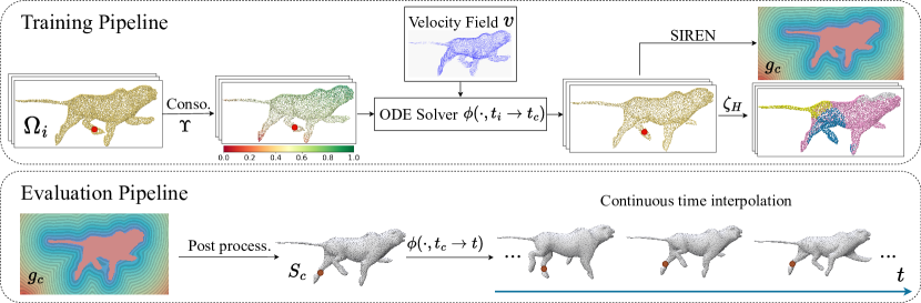
Figure 2. Our training and evaluation pipelines. In the training phase, the sequence of input point clouds $\Omega=\{\Omega_{i}\}$ is first adapted with the learnable dynamic consolidator module $\Upsilon$, which deforms points to reduce variance and provides confidence scoring (in color). The result is fed, along the learnable velocity network $v$, to an ODE solver that produces the flow $\phi$ which transforms the points to the canonical time $t=c$. The points are segmented with the learnable motion-segmentation network $\zeta_{H}$ to discover their articulation, and reconstructed with SIREN to form the implicit canonical function $g_{c}$. Our losses train these modules accordingly. Our evaluation pipeline first extracts the zero set $S_{c}$ of $g_{c}$ by marching cubes, remesh it in post-process to any desirable discretization $M_{c}$, and then uses the ODE solver to flow its vertices into shape $S_{t}$ for any prescribed time $t$.

3. Methodology

3.1. Representation

Input and Output

Our input comprises a time-stamped series of $N$ point clouds $\Omega=\left\{\Omega_{i}\right\},\ \Omega_{i}=\left\{\mathcal{P}_{i},\mathcal{N}_{i},t_{i}\right\}$ for $i\in[1,N]$, where $\mathcal{P}_{i}=\left\{x_{i,j}\in\mathbb{R}^{3}\right\}$ are individual point clouds, $\mathcal{N}_{i}=\left\{n_{i,j}\in\mathbb{S}^{2}\right\}$ are corresponding normals, and $t_{i}\in[0,1]$, so that $t_{1}=0$, $t_{N}=1$, and $\forall i,t_{i+1}>t_{i}$. We sometimes omit the point-cloud index $i$ to note point $x_{j}$ and $n_{j}$ for clarity when it is obvious from the context. Our working assumption is that point clouds represent a sampling of an unknown single deforming closed $2$-manifold surface $S(t)$ of an arbitrary topology, where its topology is constant over time. The sampling is independent for each time frame, and the point clouds are not assumed to correspond between frames; they can also vary in size and noise level.

Our output is a function $f(x,t):\mathbb{R}^{3}\times\mathbb{R}\rightarrow\mathbb{R}$ that represents $S(t)$ implicitly by its dynamic zero sets. Formally, define the single frame function $g_{t}(x)=f(x,t)$, then $S_{t}=g_{t}^{-1}(0)$.

Representing coherency with flows

As pointed out by (Eckstein et al., 2007; Atzmon et al., 2021; Stam and Schmidt, 2011; Tao et al., 2016), the implicit function $f$ can only describe the shape at every time point, but not unambiguously encode the pointwise deformation of $S_{t}$ through time: the tangential components of the deformation cannot be unambiguously inferred. Without the explicit deformation, a purely implicit representation would fail at a coherent and physically plausible interpolation of motion, and would consequently fail at completing missing regions or noise, or maintaining a consistent topology. See Fig. 14 and Fig. 15 for such examples. To counter this, we represent $f$ by decoupling it into two components:

1. Canonical shape: we pick the time $c=0.5$, in which we define $g_{c}(x):\mathbb{R}^{3}\rightarrow\mathbb{R}$ as the implicit canonical function, and where then the canonical shape is $S_{c}=g_{c}^{-1}(0)$.

2. Flow velocities: we define the velocity $v(x,t):\mathbb{R}^{3}\times\mathbb{R}\rightarrow\mathbb{R}^{3}$ of every point $x$ at time $t$, with which we advect $S_{c}$ through time.

Backward and forward flow maps

From the given velocity field $v(x,t)$, we can define a forward map $\phi^{\rightarrow}(x,t)$ such that a given point $x$ at time $0$ flows to point $y$ at time $t$ when:

$$\begin{cases}\frac{\partial\phi^{\rightarrow}(x,\tau)}{\partial\tau}&=v(\phi^{\rightarrow}(x,\tau),\tau),\ \ \tau\in[0,t)\\ \phi^{\rightarrow}(x,0)&=x\\ \phi^{\rightarrow}(x,t)&=y.\end{cases}$$

Similarly, we can define the backward map $\phi^{\leftarrow}(y,0)=x$ as in (Deng et al., 2023). Rather than represent $\phi^{\rightarrow}$ and $\phi^{\leftarrow}$ as independent functions, we only represent the velocity $v$, and numerically integrate it into the forward and backward flow. We do this by an off-the-shelf differential ODE solver that becomes part of our pipeline (Fig. 2). This allows us to track the flow of each point from each time frame automatically; as such, and for clarity, we abstract the flow map to the notation: $\phi(x,t\mapsto c)$ to denote the flow of point $x$ from any time $t$, before or after the canonical time $c$, to time $c$. During the evaluation phase, we use the opposite $\phi(x,c\mapsto t)$ to flow the canonical shape to all time frames.

Our definition of $f$ at time $t$ then comprises the pullback of $g_{c}$ by $\phi$ as follows:

$$f(x,t)=g_{c}\circ\phi(x,t\mapsto c)$$

This model mixes an implicit representation by $g_{c}$, and an explicit representation of deformation by integrating $v$ into $\phi$. Combining both for the high-fidelity reconstruction of deforming geometry allows us to introduce geometric priors that have the following advantages:

1. Integrating the velocity $v$ allows us to model the deformation explicitly, and thus naturally track any point through time, independent of any mesh used to represent $S_{t}$ (Figs. 1 and  19). Furthermore, representing the velocity avoids the need to train two flow networks and consequently avoids maintaining their cycle consistency (as in e.g., (Liu et al., 2024)).

2. The reconstruction of $g_{c}$ at the time point $c$ allows us to aggregate all samples from all time frames, by advecting them through the flow $\phi$. This consolidation allows us to aggregate geometric details from all time frames even with missing regions (Fig. 14), noise (Fig. 15), or sparse point clouds (Fig. 18).

3. Using an implicit representation for $g_{c}$ allows for inferring the original topology of $S$, for any possible such topology.

4. Finally, the decoupling of $g_{c}$ and $v$ allows for a hybrid representation: $g_{c}$ can be detailed and high-frequency, whereas the deformation $\phi$, capturing the motion of a physical object, is typically low-frequency. This is evident in all our examples.

3.2. Pipeline

Training pipeline

Given the input time-framed point clouds, our architecture is illustrated in Fig. 2 (top). Its goal is to train the velocity network $v$, and the canonical shape function $g_{c}$. Other than the ODE solver, the components in our training architecture are:

1. A dynamic consolidator module that adapts the input point clouds for a more coherent fitting (Sec.  6).

2. A velocity network $v$ that simulates the smooth and physically-plausible deformation (Sec. 4).

3. A SIREN-based (Sitzmann et al., 2020) implicit reconstruction module producing $g_{c}$. (Sec. 5).

4. A motion-segmentation network that segments the canonical shape, for a piecewise articulation of deformation. (Sec. 4.2).

Our training paradigm trains $g_{c}$ and $v$ simultaneously, with the following objectives:

• We fit the signed distance function $f(x,t)$ to each point cloud $\Omega_{i}$, as a composition of $g_{c}$ and the flow $\phi$, integrated from the velocity $v$ (Sec. 5).

• We regulate the spatial and temporal derivative of the velocity (Sec. 4).

Evaluation pipeline

Having trained the velocity network $v(x,t)$ and the implicit canonical function $g_{c}$, and given any prescribed time $t\in[0,1]$, we evaluate and output $S(t)$ as follows (Fig. 2 bottom):

1. Produce a mesh $M_{c}$ to discretize the explicit canonical shape $S_{c}$, at the canonical time $c$. We first extract a triangle mesh with marching cubes (Lorensen and Cline, 1998), and then remesh it to any desired mesh.

2. Flowing the vertices of $M_{c}$ through $\phi$, by the ODE solver, to obtain $M(t)$ (as a discrete representation of $S(t)$) as the output.

A major advantage of flow-based methods like ours is that the discretization $M_{t}$ is only done at the evaluation stage, and thus entirely decoupled from the training of $g_{c}$ and $v(x,t)$. We can then make an independent and design choice for this discretization, that does not bias our training (Fig. 19). We next detail the specific components of both the training and the evaluation pipelines. We then detail the complete aggregated loss function in Sec. 6.

4. Velocity Field Design

We next describe the design choices we make for the velocity field. The architecture of our velocity network is presented in Fig. 3, and explained in the following.

4.1. Smooth Representation

We guide the design of both our representation and our regularization loss terms by the following assumptions about the velocity fields:

• They are slowly varying both in space and in time.

• They describe the physical motion of a solid (or articulated) object, and thus favor isometric or elastic deformations.

Positional encoding

Consider a single coordinate $\eta=(x,t)\in\mathbb{R}^{4}$, coefficients $b_{i}\in\mathbb{R}^{4}$ that are sampled randomly from a multivariate Gaussian distribution, and a prescribed bandwidth $d\in\mathbb{N}$. Our Random Fourier Feature (RFF) $\gamma:\mathbb{R}^{4}\rightarrow\mathbb{R}^{d}$ that encodes the space-time coordinate $\eta$ is as follows (Fig. 3):

(1) $$\gamma(\eta)=[cos(b_{1}^{T}\eta),sin(b_{1}^{T}\eta),...,cos(b_{d/2}^{T}\eta),sin(b_{d/2}^{T}\eta)].$$

As $b_{i}$ are small (we set the variance $\sigma=0.4$ for the Gaussian distribution in our experiment), this encoding serves as a Fourier basis of our space-time domain, filtering out high frequencies.

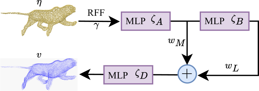
Figure 3. Our velocity network architecture, using positional encoding $\gamma$, and comprising the composition of low- and medium-frequency components controlled by weights $w_{M}$ and $w_{L}$, and followed by a decoder network to produce a spatial velocity field.

Velocity representation

We bias the representation towards a mixture of low- and medium-frequency velocities. With this, we mitigate deformation kinks and abrupt changes. In addition to the Fourier encoding in space-time coordinates, we use a mixture of two neural networks to represent the velocity field itself (see Fig. 3). Consider two fully connected single-layer networks $\zeta_{A}:\mathbb{R}^{d}\rightarrow\mathbb{R}^{h}$ and $\zeta_{B}:\mathbb{R}^{h}\rightarrow\mathbb{R}^{h}$ and with $h=512$. The network is defined as follows:

(2) $$\zeta_{LM}(\eta)=w_{M}\zeta_{A}(\gamma(\eta))+w_{L}\zeta_{B}(\zeta_{A}(\gamma(\eta))).$$

These MLP layers are activated by a SoftPlus (Dugas et al., 2000) function. The purpose of this composition is to use the smooth attenuation bias of neural networks, where $\zeta_{B}\circ\zeta_{A}$ serves as a low-frequency component; using it alone (i.e., $w_{M}=0$) would result in the loss of small details in the deformation. Using $\zeta_{A}$ alone (i.e., $w_{L}=0$), as the medium-frequency component, results in failure to capture global motion. In Fig. 4, we ablate these weights and demonstrate that the average weighting (i.e., $w_{L}=w_{M}=0.5$) is a successful choice, even when compared to the conventional skip connection $w_{L}=w_{M}=1$.

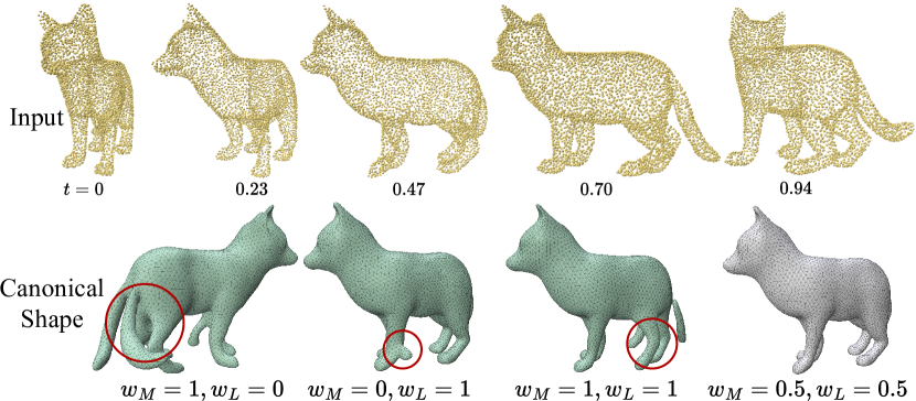
Figure 4. Given sequential point cloud inputs, different canonical shapes can be reconstructed when setting different $w_{M}$ and $w_{L}$ values. Experimentally, an average weighting scheme works the best, and we adopt it throughout our experiments.

Finally, a coordinate-based velocity decoder network (a single MLP layer) $\zeta_{D}:\mathbb{R}^{h}\rightarrow\mathbb{R}^{3}$ converts the output of $\zeta_{LM}$ into the field $v\in\mathbb{R}^{3}$.

4.2. Velocity Loss Functions

We next describe the components of the full loss function (Eq. 13) that regulate the deformation defined by the velocity field. All quantities use spatial ($x$) and temporal ($t$) derivatives of the velocity $v$ obtained by auto differentiation.

Isometric Energy

We use the Killing energy (Solomon et al., 2011; Tao et al., 2016; Slavcheva et al., 2017) as a first-order approximation for isometry. The killing energy of our velocity field $v(\cdot,t)$ at any time step $i$ is defined as:

(3) $$E_{\text{kill}}(i)=\frac{1}{2}\mathbb{E}_{x_{j}\in\mathcal{P}_{i}}\left\lVert\nabla v(x_{j},t_{i})+\nabla v(x_{j},t_{i})^{T}\right\rVert_{F}^{2},$$

where $\mathbb{E}$ denotes the average (expectancy) over each point cloud $\mathcal{P}_{i}$, and using the Frobenius 2-norm. $\nabla$ denotes the partial derivative of the spatial coordinates.

Dirichlet Energy

We also regulate the spatial variation of the deformation by introducing a Dirichlet energy as follows:

(4) $$E_{\text{diri}}(i)=\frac{1}{2}\mathbb{E}_{x_{j}\in\mathcal{P}_{i}}\left\lVert\nabla v(x_{j},t_{i})\right\rVert_{F}^{2}.$$

Consistent Speed. Consecutive frames may be unevenly spaced in time, which might result in sudden movement or stopping artifacts (Fig. 13). Thus, we regularize the speed of the deformation with

(5) $$E_{\text{speed}}(i)=\frac{1}{2}\mathbb{E}_{x_{j}\in\mathcal{P}_{i}}\left\lVert\frac{\partial v(x_{j},t_{i})}{\partial t}\right\rVert^{2}.$$

Articulated Rigidity

Following (Atzmon et al., 2021; Zhang et al., 2023), physical objects, especially live creatures, tend to move in (softly) rigid semantic parts, such as the limbs between the joints. These kinematic units constitute a quasi-articulated system. For this, we adapt a motion-segmentation module from (Zhang et al., 2023). For a prescribed number of segments $H=20$, we learn a motion-segmentation network that is implemented as a neural field $\zeta_{H}:\mathbb{R}^{3}\rightarrow[0,1]^{H}$, that for each location $x$ in the space of the canonical time $c$ outputs a probability $\zeta_{H,h}(x)$ of the point $x$ belonging to segment $h$ (as a partition of unity: $\sum_{h}{\zeta_{H,h}(x)}=1$). We add a loss term that regularizes the per-part rigidity, by computing a pair of the rotation matrix and translation vector $\left\{R_{h,i}\in SO(3),\ \tau_{h,i}\in\mathbb{R}^{3}\right\}$ per each segment $h$ and time frame $i$, where we seek that the flow from $t_{i}$ to $c$ is as-(part-wise)-rigid-as-possible (Sorkine and Alexa, 2007), weighted by the probability of $h$:

(6) $$\begin{split}E_{\text{rigid}}(i)=\mathbb{E}_{x_{j}\in\mathcal{P}_{i}}\sum_{h\in[1,H]}\zeta_{H,h}(\phi(x_{j},t_{i}\mapsto c))\\ \cdot\left\lVert(R_{h,i}x_{j}+\tau_{h,i})-\phi(x_{j},t_{i}\mapsto c)\right\rVert^{2},\end{split}$$

In each iteration, we compute the rigid transformation $\left\{R_{h,i},\tau_{h,i}\right\}$ in closed-form by SVD of the correlation matrix between the segment at time $t$ and that of time $c$ (the classical ARAP local step). As a by-product of this training, we get a segmentation of the moving object, by considering the highest probability of each point (Fig. 5).

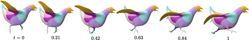
Figure 5. The motion-segmentation network learns the articulation of the object, and segments the (softly) piecewise-rigidly moving parts (different colors).

5. Fitting the 4D Function

We next introduce the fitting loss terms that govern both the reconstruction of the canonical function $g_{c}$ and the velocity field $v$. We choose to represent $g_{c}$ using SIREN  (Sitzmann et al., 2020). We find that using periodic (trigonometric) activation functions instead of ReLU tends to capture finer details, ensuring accurate fitting within our context.

Fitting SDFs

During the training stage, our 4D function $f(x,t)$ is obtained by the integration of velocity $v$ (through the ODE solver) which determines the deformation of points from the times $t_{i}$ to the canonical time $c$. We would like $f(x,t_{i})$ to be a signed distance function (SDF) for each time frame $t_{i}$, where its zero set should be fit to the point cloud $\mathcal{P}_{i}$, and its gradient should be fit to the normals $\mathcal{N}_{i}$. Therefore, our fitting loss is defined as:

(7) $$\begin{split}E_{\text{fit}}(i)=\mathbb{E}_{x_{j}\in\mathcal{P}_{i}}(|f(x_{j},t_{i})|^{2}+\lambda_{n}\left\lVert\nabla f(x_{j},t_{i})-n_{i,j}\right\rVert^{2}),\end{split}$$

where $n_{i,j}$ is the normal to point $x_{i,j}$ at time frame $i$, and $\lambda_{n}=0.1$ is a hyperparameter that governs the balance of zeroth- to first-order fitting. We further introduce an Eikonal term to control the unit-gradient property of SDFs anywhere. Given a sampling $\mathcal{Q}_{i}=\left\{q\right\}$ of points in the unit bounding box, at every time frame $i$ we define:

(8) $$E_{\text{eik}}(i)=\mathbb{E}_{q\in\mathcal{Q}_{i}}(\left\lVert\nabla f(q,t_{i})\right\rVert-1)^{2},$$

where $\mathcal{Q}$ is a sum of uniform sampling of $10K$ points inside the bounding box of $\Omega$, replaced in each iteration, and a mixture Gaussian distribution sampled near the point cloud. Concretely, one point in the latter distribution $q=x_{i,j}+\epsilon$ is sampled by adding a random displacement $\epsilon$, which is drawn from a mixture of two Gaussians, $\mathcal{N}(0,\sigma^{2}_{1}I)$ and $\mathcal{N}(0,\sigma^{2}_{2}I)$. The parameter $\sigma^{2}_{1}$ depends on each $x$ and is set to be the distance of the $10^{th}$ closet point to $x$, whereas $\sigma_{2}$ is set to a fixed $0.3$.

6. Dynamic Consolidator Module

Our fitting process is inherently ill-defined in that it tries to fit both the canonical shape and the velocity field simultaneously, without any other source of supervision. As such, inaccuracy in either the canonical fitting or the velocity field will easily manifest throughout the entire 4D reconstruction. A common example of such an artifact is an inaccurate registration of the advected point clouds at the canonical time, which might result in a shape that is a superposition of several shapes at once (see Fig. 17).

A chief reason for this artifact is weak signals on how to fit in-flowing shapes in the space of time $c$. This is especially true for fast-moving shapes, or with considerable noise and outliers in the input. It is common for backward-flow methods (Park et al., 2021; Sun et al., 2022; Niemeyer et al., 2019; Pumarola et al., 2021) to mitigate this by balancing the deformation function and the canonical implicit shape with repeated adjustments to the learning rate. However, there is an inherent source of inaccuracy and non-robustness in flow-based methods: the canonical shape is always decided by all point clouds, after advecting them to the canonical time. However, the flow is a learned quantity (potentially through learning the velocity field), and thus suffers from the smooth bias of networks, where the result is the flow from nearby time frames is considerably more correct in early iterations than that from the farthest frames. This causes an error in the registration from the distant frames. A mechanism to adaptively suppress the signals for the farthest frames, and rate their confidence, is thus required.

Our approach to dealing with these issues is introducing a learnable transformation of the input between the raw input and the rest of the pipeline. In addition, we add a learnable confidence-based weighting to the fitting process that dynamically dilutes the effect of outliers during the fitting process. Formally, we introduce a learnable dynamic consolidator module $\Upsilon:\mathbb{R}^{4}\rightarrow\mathbb{R}^{4}$ that has two outputs as follows:

(9) $$\Upsilon:(\eta_{i,j}|\theta_{i})\rightarrow(x_{i,j}+\delta_{i,j},p_{i,j}),$$

$\eta_{i,j}=(x_{i,j},t_{i})$ is the space-time coordinate of point $j$ in cloud $\mathcal{P}_{i}$, and $\theta_{i}\in\mathbb{R}^{128}$ is an independent learnable consolidator latent code for this cloud. One branch $\delta$ of the consolidator module $\Upsilon$ returns a small spatial deviation function $\delta_{i,j}=\delta(x_{i,j})$ to the raw data input. The other branch $p$ returns a confidence score function $p_{i,j}=p(x_{i,j})\in[0,1]$ for each input point $x_{i,j}$. With this, the function $f$ can be redefined as:

(10) $$\widehat{f}(x,t)=g_{c}\circ\phi(x+\delta,t\mapsto c).$$

The role of the deviation function $\delta$ is to transform the input points so that the consolidation of the point cloud at the canonical time $c$ is more homogeneous and amenable to fitting $g_{c}$. The confidence $p_{i,j}$ measures confidence at that point. We reformulate the corresponding fitting loss as follows:

(11) $$\widehat{E}_{\text{fit}}(i)=\mathbb{E}_{x_{j}\in\mathcal{P}_{i}}(p_{i,j}(|\widehat{f}(x_{j},t_{i})|^{2}+\lambda_{n}\left\lVert\nabla\widehat{f}(x_{j},t_{i})-n_{i,j}\right\rVert^{2})).$$

Regulating $\Upsilon$

Our scheduling of the training process is such that at the first $20\%$ of the training iterations (see concrete details in Sec. 7.1), we allow the dynamic consolidator to learn $\delta$ and $p$ with little regularization, and then gradually regulate it more to let it converge to the original input points. We regulate $\delta$ both in magnitude and in smoothness, with the following two loss terms:

$$E_{\text{mag}}(i) =\mathbb{E}_{x_{i,j}\in\Omega}||\delta_{i,j}||_{2}^{2}$$

$$E_{\text{var}}(i) =\mathbb{E}_{x_{i,j}\in\Omega}||\nabla\delta_{i,j}||_{F}^{2}.$$

In addition, we use the following log-likelihood loss to encourage the fitting to use all points from the raw consecutive frames:

(12) $$E_{\text{log}}(i)=-\mathbb{E}_{x_{j}\in\mathcal{P}_{i}}log(p_{i,j}),$$

which is zero if and only if all confidences are $1$.

Total energy

Finally, our complete energy function is as follows:

$$E(i)= \lambda_{\text{fit}}\widehat{E}_{\text{fit}}(i)+\lambda_{\text{eik}}E_{\text{eik}}(i)+\lambda_{\text{mag}}E_{\text{mag}}(i)+$$

$$\lambda_{\text{var}}E_{\text{var}}(i)+\lambda_{\text{log}}E_{\text{log}}(i)+\lambda_{\text{kill}}E_{\text{kill}}(i)+$$

$$\lambda_{\text{diri}}E_{\text{diri}}(i)+\lambda_{\text{speed}}E_{\text{speed}}(i)+\lambda_{\text{rigid}}E_{\text{rigid}}(i),$$

(13) $$E= \sum_{i}{E(i)}.$$

The first five terms are for the canonical fitting (Sec. 5), while the last four are for regulating the vector field (Sec. 4). $\lambda$ are hyperparameters that are scheduled as explained in Sec. 7.1.

Discussion

Our dynamic consolidator module embodies the adversarial training paradigm: To decrease the fitting loss, the dynamic consolidator is pushed to raise $\delta$ so that $f$ overfits the transformed point clouds as much as possible, producing smoothed motion. As training iterations increase, we keep raising the regularization weights $\lambda_{\text{mag}}$, $\lambda_{\text{var}}$, and $\lambda_{\text{log}}$. They in turn push back by reducing the magnitude and variance of the consolidator output, encouraging the optimization to better fit the original points and motion gradually. Together, they strike a balance to fit the original shape well, while effectively filtering out outliers and noise, and covering for missing regions. See Figs. 14, 15 and  17 for such examples. We note that 4D-CR (Jiang et al., 2021), while as a whole incompatible with our method, has a different approach for regulating consolidation that might have potentially fit our cause, but is not as effective; we ablate it in Sec 7.3.

7. Results and Evaluation

7.1. Implementation details

Code and hardware

We run all our experiments on a single NVIDIA A100 80GB GPU. Our code is based on PyTorch (Paszke et al., 2019) and uses the torchdiff (Chen, 2018) package to implement the ODE solver. We use Polyscope (Sharp et al., 2019) for visualization.

Dynamic consolidator

Our dynamic consolidator (Sec. 6) is built as illustrated in Fig. 6, where it accepts a spacetime coordinate $\eta=(x,t)$, and is conditioned on a learnable latent code $\theta$, to produce the outputs $\delta$ and $p$.

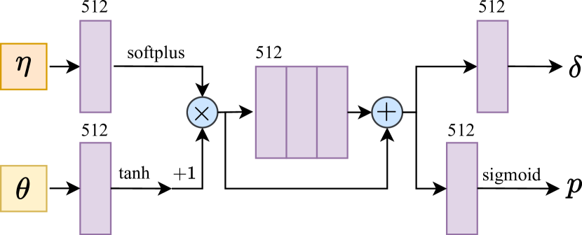
Figure 6. The dynamic consolidator. The inputs are the 4D position $\eta$ and learnable latent code $\theta$, and the output is the perturbation $\delta$ and the confidence $p$. The rectangles are MLP layers of 512 neurons.

ODE Solver

To integrate the flow $\phi$ from the velocity $v$, we use the Dormand–Prince method ’dopri5’ (Dormand and Prince, 1980), setting relative and absolute error tolerances to ${1}\mathrm{e}{-3}$ and ${1}\mathrm{e}{-5}$, respectively.

Hyperparameters and scheduling

Our experiments are run for 15000 full learning iterations. We implement a scheduling strategy for the velocity-network regularization weights $\lambda_{\text{kill}}$, $\lambda_{\text{diri}}$, and $\lambda_{\text{speed}}$ (Sec. 4.2) as follows: they are initially set to 0 for the first $7000$ iterations (during which we do not compute the unused associated derivatives); by doing so, the velocity field is only guided by $\widehat{E}_{\text{fit}}$, $E_{\text{eik}}$ and $E_{\text{rigid}}$. We subsequently increase them as follows: from $\lambda_{\text{kill}}={5}\mathrm{e}{-5}$, $\lambda_{\text{dir}}={8}\mathrm{e}{-5}$, and $\lambda_{\text{speed}}={1}\mathrm{e}{-3}$ to ${1.5}\mathrm{e}{-3}$, ${3.8}\mathrm{e}{-3}$, and ${2}\mathrm{e}{-2}$ respectively and uniformly over the next $5000$ iterations. We then maintain them at ${5}\mathrm{e}{-4}$, ${6.5}\mathrm{e}{-4}$, and ${5}\mathrm{e}{-3}$ respectively for the final $3000$ iterations. We set the fixed $\lambda_{\text{rigid}}={1}\mathrm{e}{3}$, based on (Zhang et al., 2023), and also set $\lambda_{\text{eik}}=0.1$. Our loss coefficients $\lambda_{\text{mag}}$, $\lambda_{\text{var}}$, and $\lambda_{\text{log}}$ for the dynamic consolidator, unless otherwise specified (e.g., Fig. 16), are initially set to $\lambda_{\text{mag}}=\lambda_{\text{var}}=0.01$, and $\lambda_{\text{log}}=0.10$ for the first $3000$ iterations. We then increase them to $0.4$, $30$, and $2.0$ respectively and uniformly over the next $9000$ iterations, maintaining these final values for the last $3000$ iterations.

We use the Adam optimizer (Kingma and Ba, 2014) with a Constant Learning Rate Schedule, reduced by $0.5$ every $500$ intervals for the velocity network. The initial learning rate for the velocity network is set to ${3}\mathrm{e}{-4}$. The initial learning rate for the SIREN decoder is ${3}\mathrm{e}{-6}$, and for all latent codes and the consolidator, it is set to ${1}\mathrm{e}{-3}$. Furthermore, for the fitting, we randomly sample 1000 points from raw 4000 points in each time frame, in each iteration.

7.2. Benchmark and Comparisons

Benchmark.

Niemeyer et al. (2019) evaluate their method on the human dataset DFAUST (Bogo et al., 2017). However, DFAUST only features simple movements performed by humans, which are not diverse enough to evaluate our model effectively. To address this, we chose 26 motion sequences from the synthetic DeformingThings4D dataset (Li et al., 2021b), covering a wide range of animal types and motions. In addition, we also select $8$ sampled consecutive frames from the cloth human motion dataset CAPE (Pons-Moll et al., 2017) as a real human action test set. For each test case, we clip and downsample (in the time axis) a subset of frames from the raw dataset, resulting in sequences of $10$ to $25$ frames per case. These frames are spatially sampled to build input sequential point clouds, which contain $4000$ points for each frame in our experiment. We provide iteration and evaluation times for our experiments in Table 4.

Baselines

We compare our method with state-of-the-art methods. In some of the following cases, the application and scope are different, but they have components that mirror ours (specifically, velocity networks). In these cases, we explain how we adapt them to fit our task:

1. NDF (Sun et al., 2022), which uses a similar reconstruction paradigm, and proposes a conditional quasi-time-varying velocity field, and uses DeepSDF to set as canonical shape representation.

2. DSR (Sun et al., 2023), which uses an SDF decoder network to predict SDF values for the spacetime input, without explicit deformation tracking.

3. OFlow (Niemeyer et al., 2019), which introduces ODE into 3D shape deformation. We adapt their proposed velocity field in our comparison, where we replace the shape and consequence identity-extracting network with two learnable latent codes. The purpose is to convert their pipeline that trains an entire dataset, to our case of fitting a single shape. Specifically, we test whether their (large) velocity network is competitive to our small one.

4. NVFi (Li et al., 2023), which model 3D scene dynamics from multi-view videos. We adapt their proposed velocity field to the OFlow pipeline described above.

Except for DSR, which is a 4D spacetime method, all other compared methods are flow-based, who first obtain the canonical shape, and then flow it to all other times. Another important difference between the flow-based methods and ours is that they all use DeepSDF (Park et al., 2019), whereas we use SIREN (Sitzmann et al., 2020). While SIREN is nominally more advanced, and promotes high-frequencies (and thus details), we empirically witness that it considerably degrades their results. We attribute this effect to the quick (in iteration number) fitting of SIREN; other methods lack a consolidator like ours, and thus when the velocity field is not well trained yet, SIREN converges prematurely on the wrong canonical shape (see Fig. 7). Our consolidator mitigates this effect for our method (see Fig. 17). As such, we use the originally-intended DeepSDF for their results, and SIREN for ours in all examples.

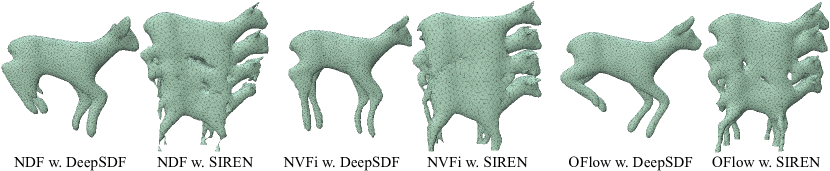
Figure 7. Using SIREN as we do considerably worsens the canonical shape of other methods, with evidently wrong consolidation.

In our visual examples, we show results from these methods, and often stress DSR more, as it is the most recent, and since its performance is the most consistently close to ours.

Setup

We synchronize all methods that use a canonical shape (not DSR) to use the same canonical time $c=0.5$. The number of iterations for NDF, NVFi, and our method is set at 15000. In contrast, we set it to 10000 for OFlow, considering its larger network parameters and training time (see Table 4) which are originally designed for training entire datasets.

Evaluation Metrics

We use the following common evaluation metrics: mean Intersection-over-union (IoU), Chamfer L1-Distance (CD), and Normal Consistency (NC). In our quantitative evaluation, we consider both the mean value and the worst score along the temporal axis, for a more rigorous evaluation. For each sequence, we interpolate 50 frames from the start time $t=0$ to the end time $t=1$, and each interpolated fitted frame is evaluated and compared against the ground truth mesh at the temporally nearest time (under the assumption that the difference is relatively negligible (as done in (Sun et al., 2023, 2022; Zeng et al., 2022)).

Results

In Table 1 and Table 2, we demonstrate that our method outperforms other methods in all metrics, both for the synthetic animals’ dataset and the real human motion datasets. We show the visual comparisons in Fig. 8 and Fig. 9, where our temporal coherency is evident by the deformation mesh. The use of SIREN as the representation for our canonical shape helps reproduce its high-frequency features. Additionally, the velocity network proposed for NDF and NVFi can not correctly align the same parts of different frames, compared to OFlow with a deep velocity network and DSR when the sequence is fast and complex (see woman in Fig. 9). However, DSR uses a single SDF network to fit all frames which results in over-smoothing and loss of details especially for the complex object (see the elephant case in Fig. 8, and the teaser Fig. 1).

Table 1. Quantitative results for the animals dataset (Fig. 8). The best method and values are bold and colored.

	Method	IoU(%)		CD($\times 10^{-4}$)		NC($\times 10^{-2}$)
		Mean$\uparrow$	Min$\uparrow$	Mean $\downarrow$	Max$\downarrow$	Mean$\uparrow$	Min$\uparrow$
	NDF (Sun et al., 2022)	74.43	58.45	14.20	70.40	75.82	68.27
	DSR (Sun et al., 2023)	75.26	69.50	6.762	15.81	77.59	72.68
	OFlow (Niemeyer et al., 2019)	78.47	71.56	8.012	32.28	77.17	72.37
	NVFi (Li et al., 2023)	75.59	68.95	12.00	44.12	75.50	71.50
	Ours w/o Consolidator	81.66	73.28	16.16	80.66	77.37	72.14
	Ours	82.84	74.12	4.606	15.28	78.21	73.37

Table 2. Quantative Results for the human data set (Fig. 9).

	Method	IoU(%)		CD($\times 10^{-4}$)		NC($\times 10^{-2}$)
		Mean$\uparrow$	Min$\uparrow$	Mean $\downarrow$	Max$\downarrow$	Mean$\uparrow$	Min$\uparrow$
	NDF (Sun et al., 2022)	79.55	59.30	14.03	84.71	82.96	73.76
	DSR (Sun et al., 2023)	80.23	77.42	10.13	14.38	83.35	81.93
	OFlow (Niemeyer et al., 2019)	77.15	73.38	28.55	35.00	81.61	80.08
	NVFi (Li et al., 2023)	81.50	75.73	21.62	25.39	82.85	80.73
	Ours	84.17	80.94	6.554	11.23	84.98	83.06

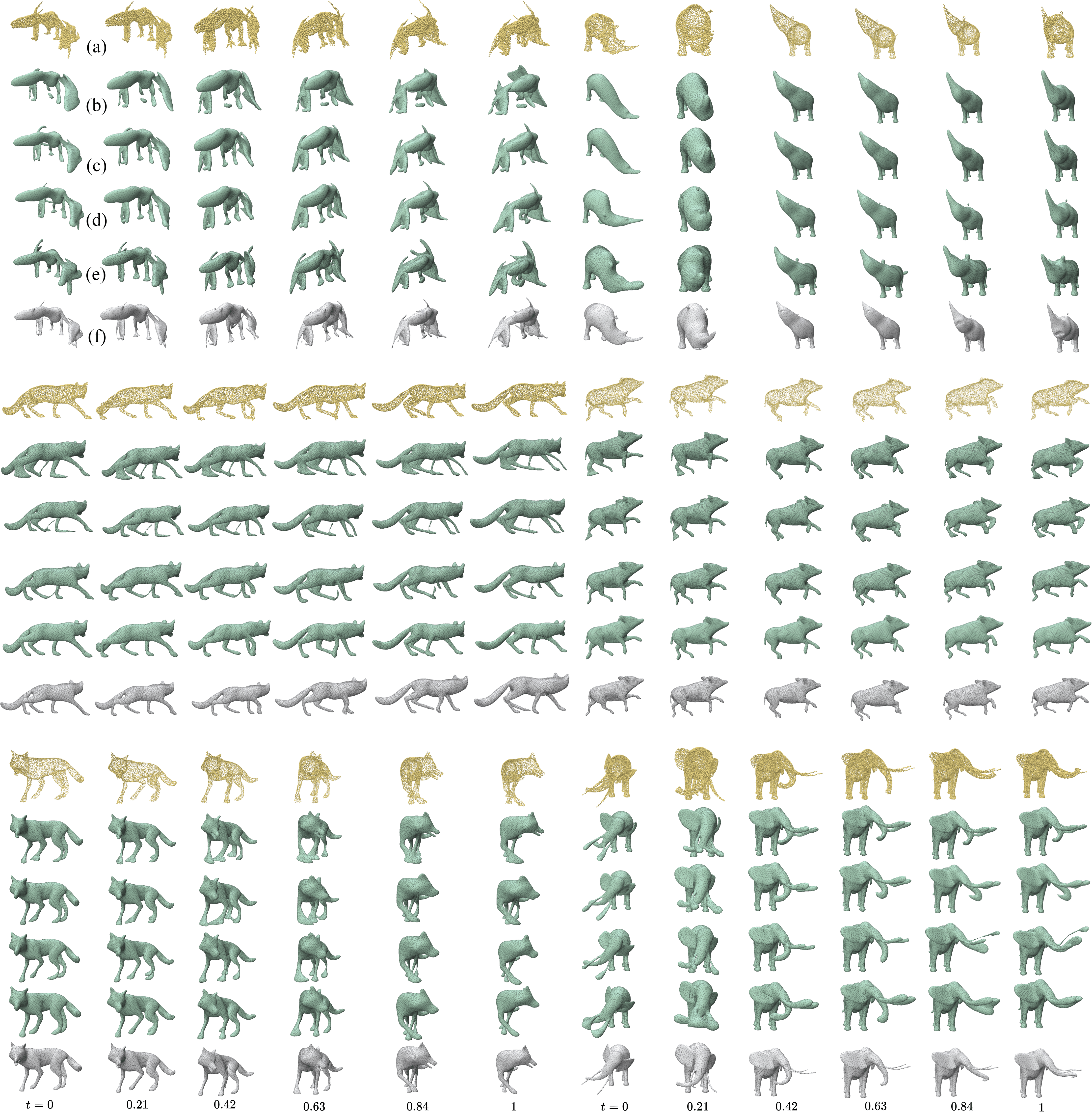
Figure 8. Qualitative results of synthetic animals motions from the Deformingthings4D (Li et al., 2021b) dataset in our experiments. (a): input sequences, (b) OFlow (Niemeyer et al., 2019)+NVFi velocity (Li et al., 2023), (c): NDF (Sun et al., 2022), (d): OFlow (Niemeyer et al., 2019), (e) DSR (Sun et al., 2023), (f) Ours. Ours reproduces a natural temporal deformation with correct spatial details without oversmoothing, or introducing topology or geometric artifacts.

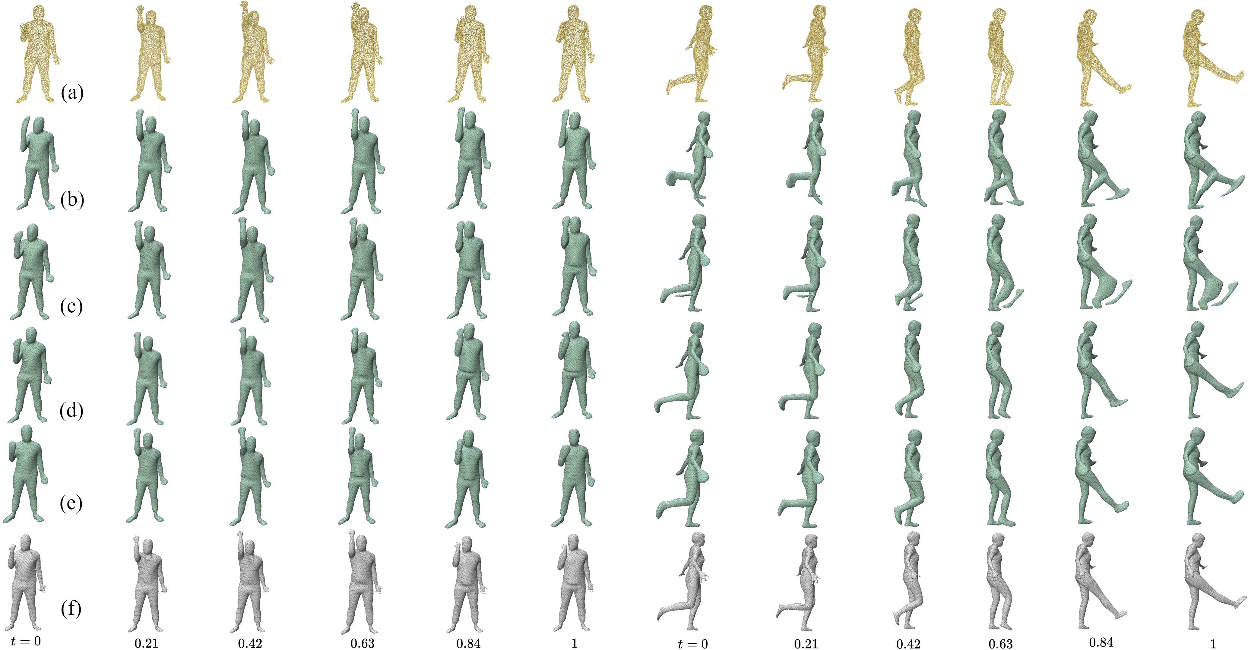
Figure 9. Qualitative results of real human motions from CAPE dataset (Pons-Moll et al., 2017). (a): input sequences, (b): OFlow (Niemeyer et al., 2019)+NVFi velocity (Li et al., 2023), (c): NDF (Sun et al., 2022), (d): OFlow (Niemeyer et al., 2019), (e) DSR (Sun et al., 2023),(f) Ours. Note again that our work is the only one that consistently reproduces both spatial and temporal details accurately.

7.3. Analysis and Ablation

We next explore how our choices of hyper-parameters, loss components, and architectural choices affect our results. We refer the reader to the video which shows animated versions of these examples.

Reproducing rigid motions

We demonstrate the importance of our Killing energy ($E_{\text{kill}}$) for reproducing isometric and rigid motions in Fig. 10. For this, we use a Genus-2 mesh from Thingi10K (Zhou and Jacobson, 2016) (ID: 83024), which we transform by a rotation around the center of mass, and sample spatially and temporally to a point-cloud sequence. We show the result in Fig. 10. It is evident that with the energy, we reproduce the motion almost perfectly, whereas without it, we get deformation artifacts.

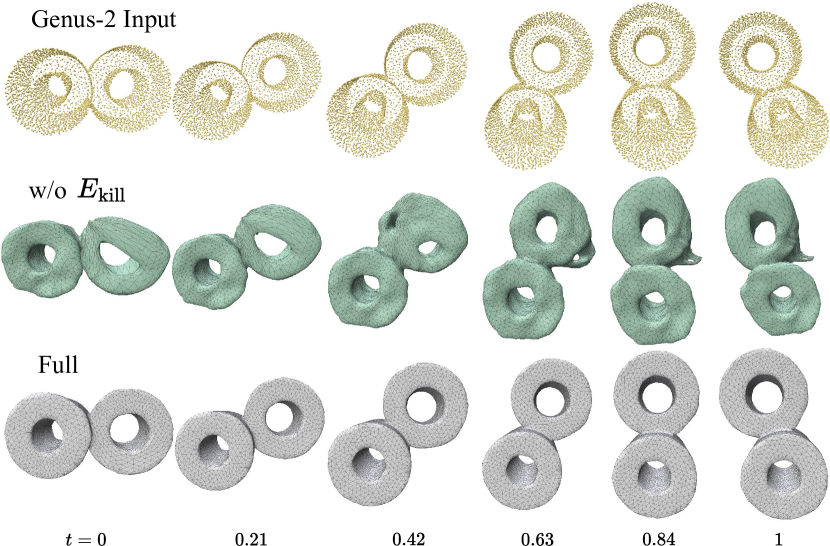
Figure 10. $E_{\text{kill}}$ encourages the reproduction of rigid transformation, reducing deformation artifacts.

Dirichlet Energy

We show how $E_{\text{diri}}$, by regulating the spatial smoothness of the deformation, can reproduce the gentle deformation of the wrist in Fig. 11, avoiding kinks and irregularities.

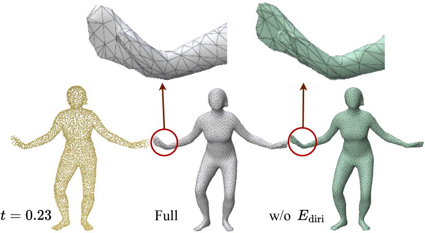
Figure 11. The Dirichlet energy $E_{\text{diri}}$ helps keep the same local shape under deformation. The unnaturally deforming parts are circled by red.

Sparse Frames

In Fig. 12, we demonstrate how our algorithm can reproduce movements smoothly even with considerably fewer frames than provided in the input. We further compare this to the performance of DSR (Sun et al., 2023) in Fig. 13. Note that DSR does not reproduce near-isometric motions during the deformation, likely since their deformation moves along the steepest gradient of the network, rather than the correct physical move. This result further ablates the speed-consistency loss term $E_{\text{speed}}$, which evidently serves to keep finer details without blur (see the rabbit eyes in Fig. 13) and reduce sparse-frame artifacts.

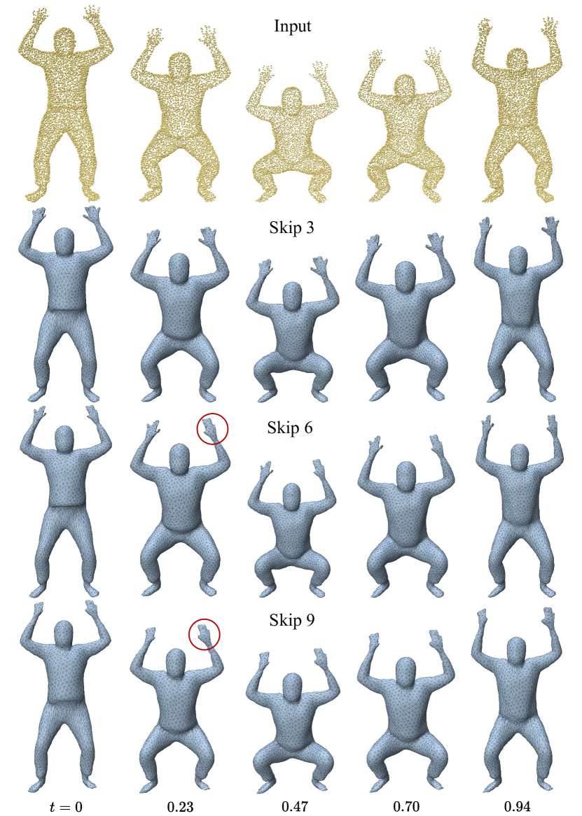
Figure 12. Our method is robust to using fewer frames. We show the results in the same (marked) interpolated time frames, where the point clouds are the closest original input. “Skip” is the stride used to temporally sample from the raw sequence (e.g., skip 3 = using frames $1,4,7,\ldots$). Our method is still able to reproduce the motion.

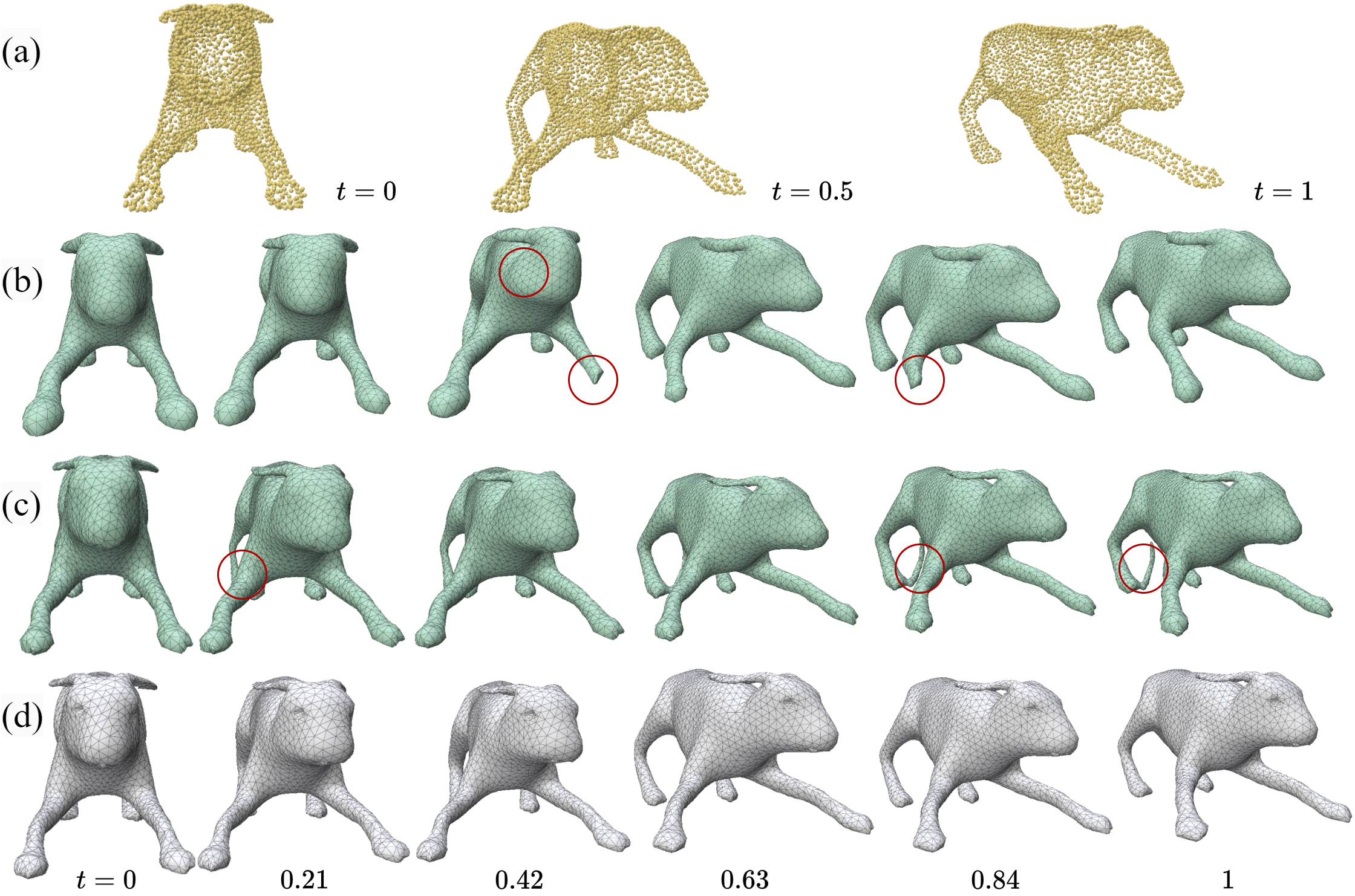
Figure 13. Our method is robust even when using only three frames of a sequence. (a) Input sequence with three frames, (b) DSR, (c) Ours w/o Consistent speed ($E_{\text{speed}}$), (d) Ours full. Artifacts are circled.

Missing Regions

To test whether our method can aggregate partial information from different frames to compensate for missing parts, we manually crop different parts for all input frames. As shown in Fig. 14. Owing to the explicit modeling of the velocity field and its regularization, our canonical frame can be completely recovered by the advection of all details along the raw sequence. We further compare this scenario with DSR, with a quantitative measure in Table 3.

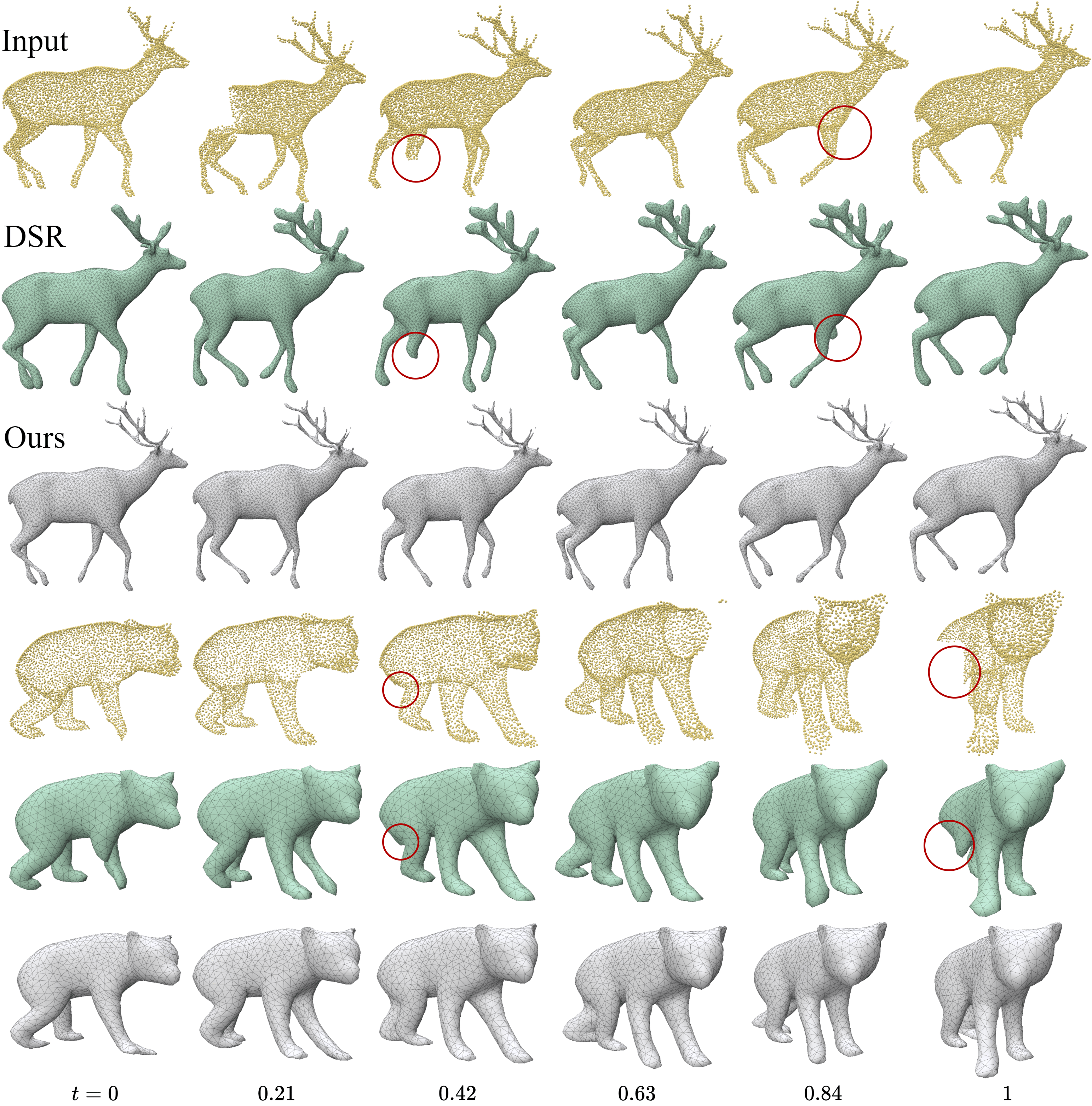
Figure 14. Our method (gray) is robust to missing regions and can recover the geometry and its deformation from other time frames effectively. The missing regions are circled in red for both raw input sequence and DSR results (green).

Table 3. Quantitative results for inputs with missing regions. The inputs are from the animals’ dataset, corresponding to Fig. 14.

	Sequence Name	Method	IoU(%)		CD($\times 10^{-5}$)
			Mean$\uparrow$	Min$\uparrow$	Mean $\downarrow$	Max$\downarrow$
	deerFEL_WalkhuntedRM	DSR(Sun et al., 2023)	80.01	74.95	65.72	168.0
		Ours	89.06	82.19	6.819	19.39
	bear3EP_WalkrightRM	DSR(Sun et al., 2023)	83.11	78.71	118.0	441.8
		Ours	89.38	86.21	36.80	90.90

Robustness to noise

We demonstrate this in Fig. 15, where we add Gaussian noises to randomly selected 4 frames out of 13 input point clouds to simulate realistic capture, with varying standard deviations, and compare against both DSR and our method without the consolidator module. The ablation shows that our consolidator module is helpful to smooth noises and then reduce artifacts, and is more robust to noise than DSR. This is as DSR produces a smooth solution that tries to fit the entire input sequence.

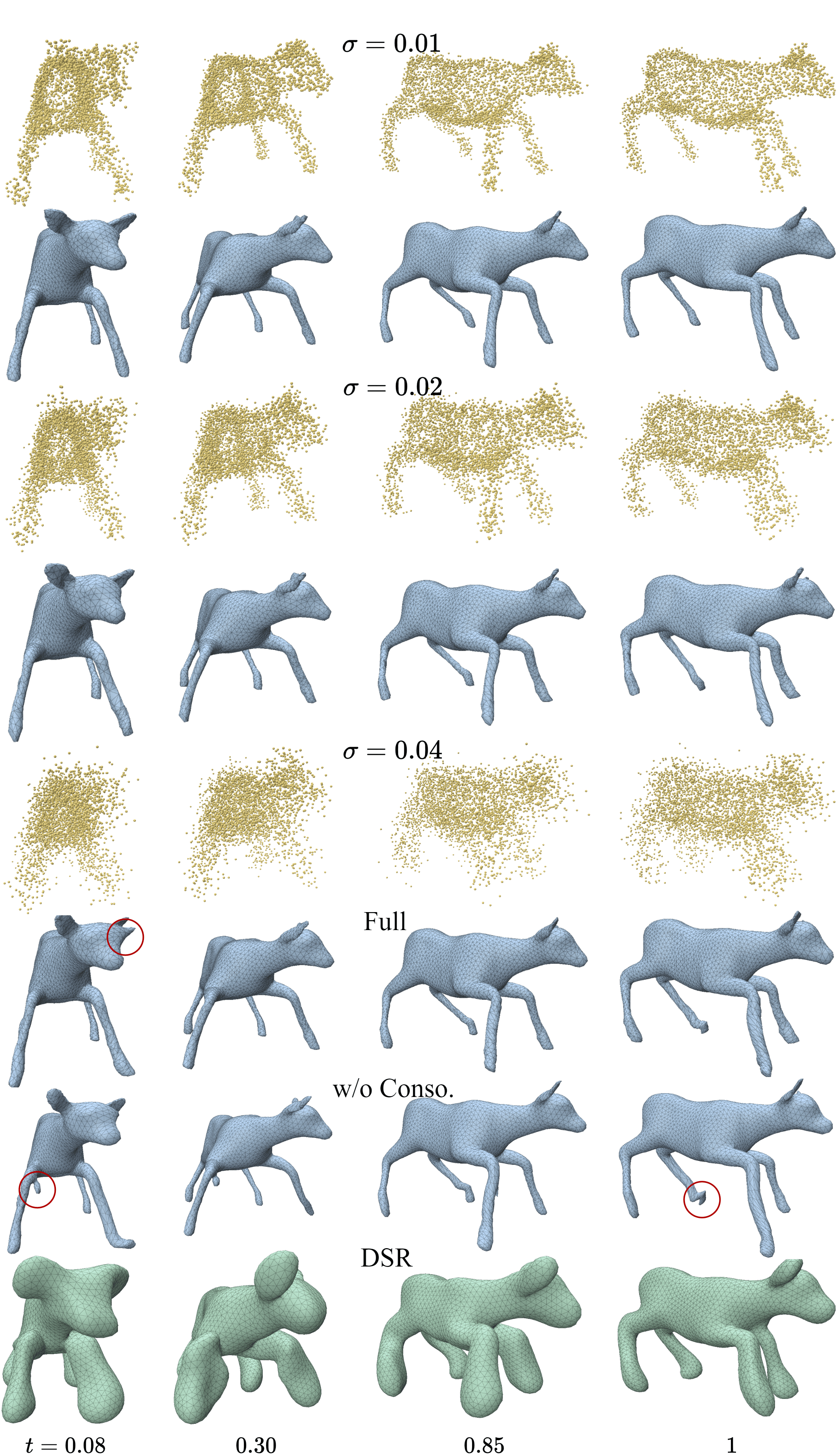
Figure 15. Our methods colored in blue is robust to different levels of noises. The green meshes are results using the $\sigma=0.04$ noisy input where the results of not using the dynamic consolidator module have artifacts, and DSR (green mesh) is easily influenced by noises. Artifacts are circled in red.

Topological artifacts

As we explain in Sec. 2, one major issue with flow-based methods, and the motivation for our consolidator module, is that they are very sensitive to errors in the inferred geometry and topology in the canonical shape. In Fig. 16 we show an example of how inferring the wrong topology in the canonical shape leads to errors in the entire deformation. The case here is that through the early-time frames, the process might mistake the hand to be connected to the sides of the body. We both compare this to our adaption of NVFi, which infers the wrong topology, and ablate this to our framework without the consolidator, which infers the proper topology, but introduces geometric artifacts. Our full framework more accurately reproduces the motion with very few artifacts. Note that here we change the default $w_{\text{log}}$ to be $0.005$, resulting in trusting the raw points a bit less in the early iteration.

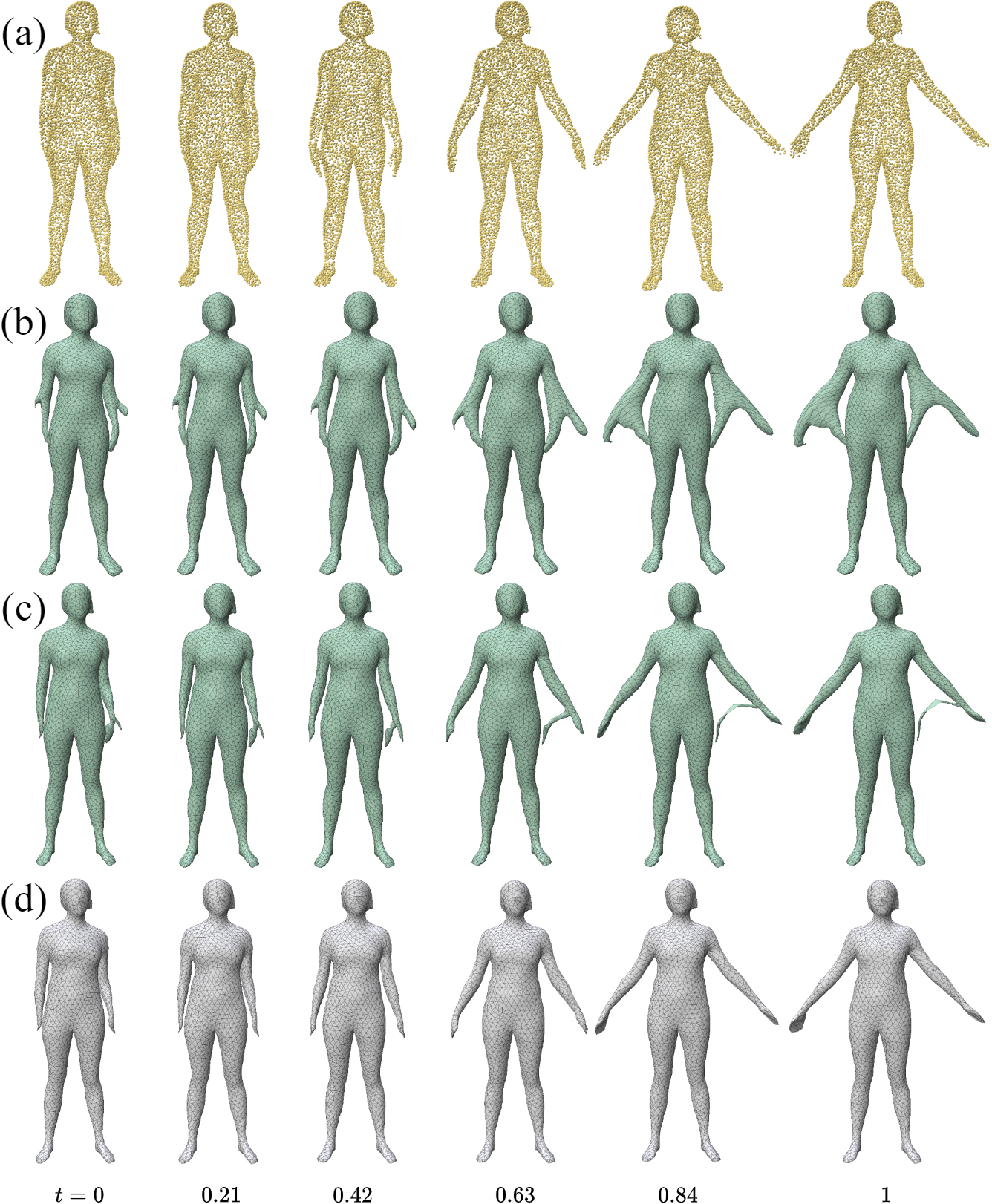
Figure 16. Our method is robust to topological artifacts inferred from the input. (a) Input sequence, (b) OFlow (Niemeyer et al., 2019)+NVFi velocity (Li et al., 2023), (c) Ours w/o consolidator, and (d) Our full method, where the default $w_{\text{log}}$ is altered to $0.005$ to keep a small fraction of points for fitting in the early stage.

Dynamic consolidator

In Fig. 17, we ablate the starting weights $\lambda_{\text{mag}}=\lambda_{\text{var}}$. Here, larger weights mean smaller deviation to the raw inputs in the early training, which results in mismatched fitting. Smaller initial weights can help alleviate the errors, especially for fast-moving during the early fitting iterations. We compare our consolidation approach to the strategy offered by 4D-CR (Jiang et al., 2021), which fails to correctly consolidate the shape. In essence, they offer to weigh the fitting energy of the canonical time against all other time frames combined: $E=E(t_{c})+\frac{1}{N-1}\sum_{i\neq c}E(t_{i})$. However, we demonstrate that this strategy is ineffective for consolidation in our examples, and specifically ablate it in Fig. 17.

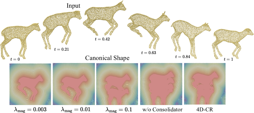
Figure 17. We ablate the initial weights $\lambda_{\text{mag}}=\lambda_{\text{var}}$ in our dynamic consolidator module. The second row depicts the implicit canonical function $g_{c}$. We choose $\lambda_{\text{mag}}=\lambda_{\text{var}}=0.01$ as the default, based on this case.

Sparser point clouds

In Fig. 18, we keep the same 14 number of frames as input and show how our method is robust to using fewer points for each frame. Even with 200 points per frame, we can still recover the correct shape and deformation, though some high-frequency details are naturally lost. This is because our consolidation effectively fills in the details. We note that using 20K points per frame in this case does not add more details—this, however, might be attributed to the SIREN representation.

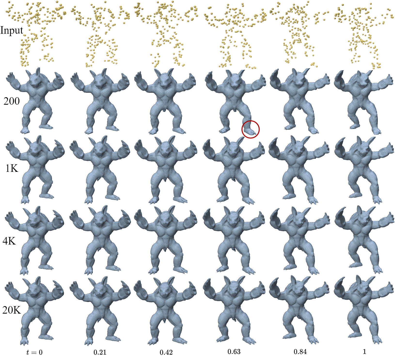
Figure 18. Our method is robust to the input with 200 points (top), albeit gradually losing details. Results with either 4k or 20k are almost indistinguishable.

Efficiency

We test timings on an A100 80G card estimated using the sequence object rabbit7L6_HiderotL, shown in Table. 4 and we also provide statistics for the learnable parameters of velocity. It is noted that NVFi has the fewest velocity parameters, but their proposed positional encoding (denoted as “velocity basis field”) of the input to the velocity field is more time-consuming, albeit with the learnable parameters. Our evaluation time for flow methods is summed by first extracting a mesh of the canonical shape by marching cubes, and then flowing this mesh to all 50 interpolated frames. In the case of DSR, one has to extract a mesh per frame individually, and thus the evaluation time is substantially higher. We note that we report average iteration time, but that our earlier iterations are considerably faster than the later ones since in the early stage we do not compute velocity derivatives.

Table 4. Comparing timings. #velo denotes the number of learnable parameters in the velocity networks (when applicable). The Fitting time is reported per 100 iterators on average.

Method	#velo$\downarrow$	FitTime(s)$\downarrow$	EvalTime(s)$\downarrow$
OFlow(Niemeyer et al., 2019)	3,291,395	83.4	42.8
NDF(Sun et al., 2022)	1,591,564	27.0	20.0
NVFi(Li et al., 2023)	70,534	36.2	24.1
DSR(Sun et al., 2023)	-	5.29	251
Ours	285,187	30.1	16.9

Different meshes

The geometric output to our method is just the implicit function $g_{c}$, which can be fitted with any desirable mesh post-process, that represents $S_{c}$. The vertices are advected with the velocity field as for triangle meshes without change. In Fig. 19, we demonstrate how our method uses different meshes with intuitive deformations. The quad mesh is obtained by using Instant Meshes (Jakob et al., 2015) from the triangle mesh of the canonical shape.

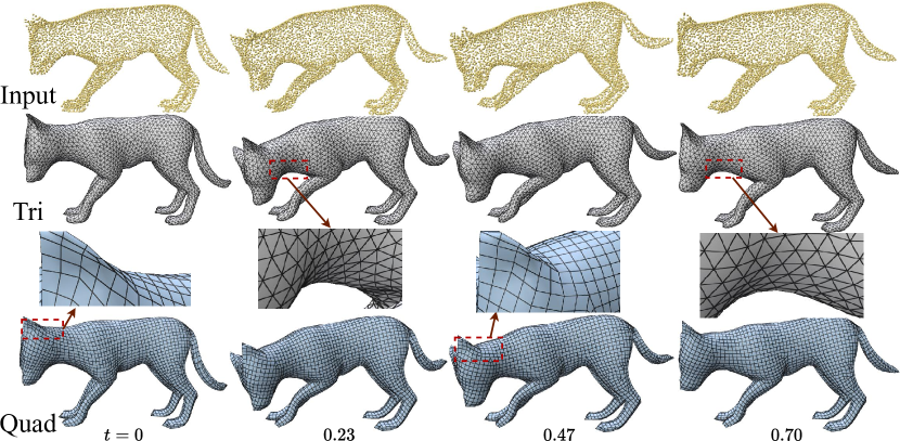
Figure 19. Our representation is invariant to post-process meshing, and we demonstrate how our deformation presents naturally for both triangle and quad meshes, where the smooth velocity does not introduce considerable tangential distortion to the mesh.

7.4. Applications

Real scan mesh

Our explicit modeling of flow can be used to advect features on geometry through time. As an example, we use the CAPE (Pons-Moll et al., 2017) raw scans with texture, where we sample 4K points for each textured raw mesh shown in Fig. 20. We then directly project the nearest raw frame textures to our fitted canonical shape per vertex by the trained velocity field and then advect the texture to different frames. We use a similar process with NVFi, and demonstrate that our texture deformation is reliable and accurate.

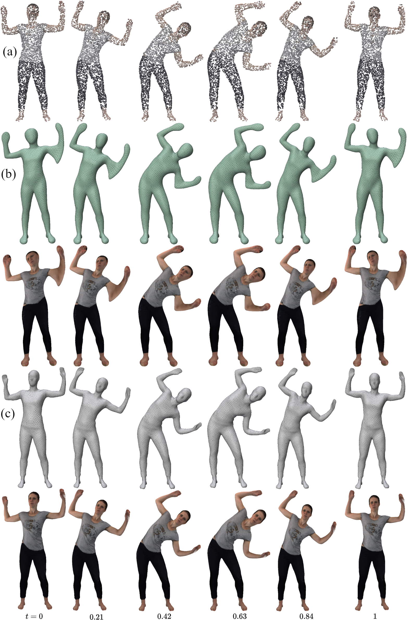
Figure 20. Raw and Textured scans. (a) The sampled 4K points from raw scans with texture. (b) The NVFi predicted results. (c) Ours. Both with and without texture.

Texturing dynamic meshes

Our work can be combined with a mesh-texturing tool. We first generate a texture from various prompts on the canonical shape, using Meshy (LLC, 2024), and then advect it through time. See Fig. 21 for the result.

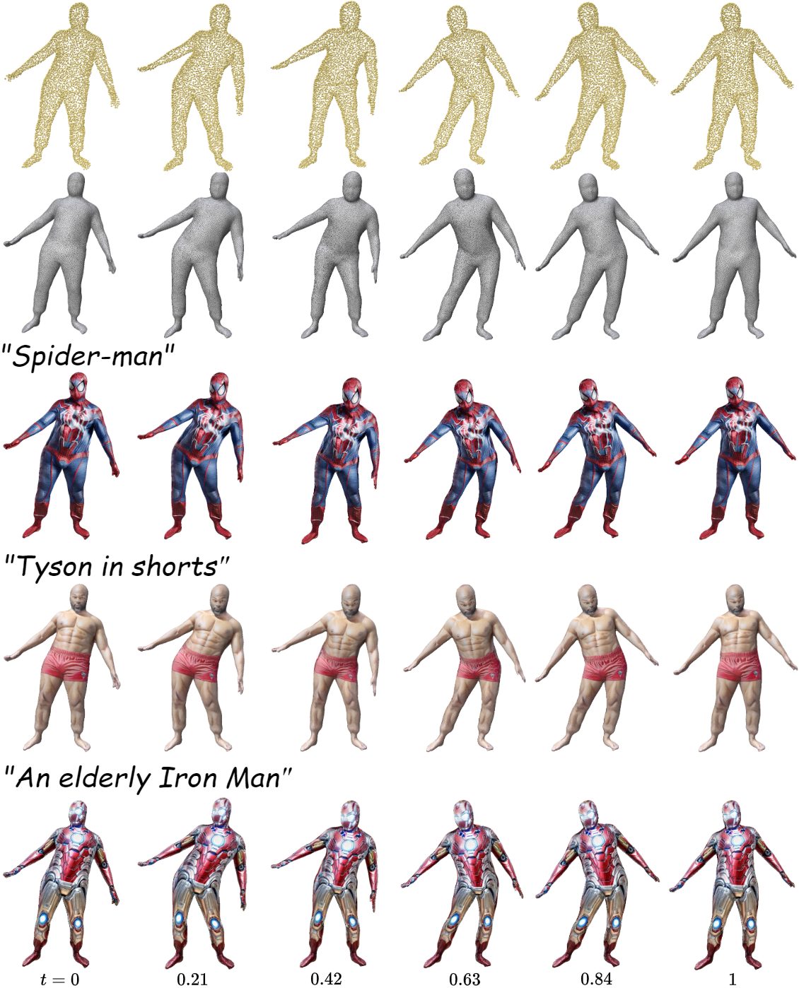
Figure 21. Our work can be used for dynamic texture generation by first generating texture for the canonical frame, and then advecting it through time.

8. Discussion

We presented a hybrid implicit-explicit scheme, with a novel consolidation process that accurately reconstructs both the geometry and the motion of a deforming object. Our results demonstrate the promise of this paradigm. Nevertheless, some issues are still left open for future work, described as follows.

8.1. Limitations

Topological changes

Purely implicit methods like DSR are inherently more general than ours, since they allow for topological changes throughout time. Keeping topology consistent through time is vital for applications like motion capture, or in general studying the deformation of a single consistent object. However, many deformations in the real world require the modeling of splitting and unification. A notable example is molecular dynamics, modeling the process of recombination of proteins and breaking of peptide bonds, which our method cannot handle. See our video for such an example.

Fast transitions

If the velocity is too fast between time frames, even if the deformation is relatively isometric and the topology is clear, our algorithm might fail to capture the correct geometry of the deforming object; see Fig. 22 for such an example. It might be that a different regularization balance can mitigate this effect, but we leave such exploration to future work.

Figure 22. A failure case for our method, where the fast movement between the middle frames introduces artifacts to the geometry (circles).

8.2. Future work

We see several possible directions for extending this work, other than those mentioned above. One interesting direction is to include textures, and other possible signals, as part of the training process itself (rather than just advect texture during the evaluation as we do in Fig. 20). This is likely to improve the consolidation. Another interesting direction is to consider different inputs that convey dynamic geometry other than point clouds, such as videos. Finally, we would like to explore the canonical consolidation presented in our work as a means to reduce a dynamic object to a representation of its articulation, that would help in automatic rigging and animation.

References

- (1)
- Atzmon et al. (2021) Matan Atzmon, David Novotny, Andrea Vedaldi, and Yaron Lipman. 2021. Augmenting implicit neural shape representations with explicit deformation fields. arXiv preprint arXiv:2108.08931 (2021).
- Ben-Shabat et al. (2022) Yizhak Ben-Shabat, Chamin Hewa Koneputugodage, and Stephen Gould. 2022. DiGS: Divergence guided shape implicit neural representation for unoriented point clouds. In Proceedings of the IEEE/CVF Conference on Computer Vision and Pattern Recognition. 19323–19332.
- Bogo et al. (2017) Federica Bogo, Javier Romero, Gerard Pons-Moll, and Michael J. Black. 2017. Dynamic FAUST: Registering Human Bodies in Motion. In IEEE Conf. on Computer Vision and Pattern Recognition (CVPR).
- Canè et al. (2018) Federico Canè, Benedict Verhegghe, Matthieu De Beule, Philippe B Bertrand, Rob J Van der Geest, Patrick Segers, Gianluca De Santis, et al. 2018. From 4D medical images (CT, MRI, and ultrasound) to 4D structured mesh models of the left ventricular endocardium for patient-specific simulations. BioMed research international 2018 (2018).
- Cao and Johnson (2023) Ang Cao and Justin Johnson. 2023. Hexplane: A fast representation for dynamic scenes. In Proceedings of the IEEE/CVF Conference on Computer Vision and Pattern Recognition. 130–141.
- Carr et al. (2001) Jonathan C Carr, Richard K Beatson, Jon B Cherrie, Tim J Mitchell, W Richard Fright, Bruce C McCallum, and Tim R Evans. 2001. Reconstruction and representation of 3D objects with radial basis functions. In Proceedings of the 28th annual conference on Computer graphics and interactive techniques. 67–76.
- Chen (2018) Ricky T. Q. Chen. 2018. torchdiffeq. https://github.com/rtqichen/torchdiffeq
- Chen et al. (2021) Zhang Chen, Yinda Zhang, Kyle Genova, Sean Fanello, Sofien Bouaziz, Christian Häne, Ruofei Du, Cem Keskin, Thomas Funkhouser, and Danhang Tang. 2021. Multiresolution deep implicit functions for 3d shape representation. In Proceedings of the IEEE/CVF International Conference on Computer Vision. 13087–13096.
- Cheng et al. (2008) Zhi-Quan Cheng, Yanzhen Wang, Bao Li, Kai Xu, Gang Dang, and Shiyao Jin. 2008. A Survey of Methods for Moving Least Squares Surfaces.. In VG/PBG@ SIGGRAPH. 9–23.
- Deng et al. (2021) Yu Deng, Jiaolong Yang, and Xin Tong. 2021. Deformed implicit field: Modeling 3d shapes with learned dense correspondence. In Proceedings of the IEEE/CVF Conference on Computer Vision and Pattern Recognition. 10286–10296.
- Deng et al. (2023) Yitong Deng, Hong-Xing Yu, Diyang Zhang, Jiajun Wu, and Bo Zhu. 2023. Fluid Simulation on Neural Flow Maps. ACM Transactions on Graphics (TOG) 42, 6 (2023), 1–21.
- Dormand and Prince (1980) John R Dormand and Peter J Prince. 1980. A family of embedded Runge-Kutta formulae. Journal of computational and applied mathematics 6, 1 (1980), 19–26.
- Dugas et al. (2000) Charles Dugas, Yoshua Bengio, François Bélisle, Claude Nadeau, and René Garcia. 2000. Incorporating second-order functional knowledge for better option pricing. Advances in neural information processing systems 13 (2000).
- Eckstein et al. (2007) I. Eckstein, J.-P. Pons, Y. Tong, C.-C. J. Kuo, and M. Desbrun. 2007. Generalized surface flows for mesh processing. In Proceedings of the Fifth Eurographics Symposium on Geometry Processing (¡conf-loc¿, ¡city¿Barcelona¡/city¿, ¡country¿Spain¡/country¿, ¡/conf-loc¿) (SGP ’07). Eurographics Association, Goslar, DEU, 183–192.
- Hanocka et al. (2020) Rana Hanocka, Gal Metzer, Raja Giryes, and Daniel Cohen-Or. 2020. Point2Mesh: a self-prior for deformable meshes. ACM Trans. Graph. 39, 4, Article 126 (aug 2020), 12 pages. https://doi.org/10.1145/3386569.3392415
- Huang et al. (2023) Jiahui Huang, Zan Gojcic, Matan Atzmon, Or Litany, Sanja Fidler, and Francis Williams. 2023. Neural Kernel Surface Reconstruction. In Proceedings of the IEEE/CVF Conference on Computer Vision and Pattern Recognition. 4369–4379.
- Huang et al. (2024) Zeyu Huang, Honghao Xu, Haibin Huang, Chongyang Ma, Hui Huang, and Ruizhen Hu. 2024. Spatial and Surface Correspondence Field for Interaction Transfer. ACM Transactions on Graphics (Proceedings of SIGGRAPH) 43, 4 (2024), 83:1–83:12.
- Jakob et al. (2015) Wenzel Jakob, Marco Tarini, Daniele Panozzo, Olga Sorkine-Hornung, et al. 2015. Instant field-aligned meshes. ACM Trans. Graph. 34, 6 (2015), 189–1.
- Jiang et al. (2021) Boyan Jiang, Yinda Zhang, Xingkui Wei, Xiangyang Xue, and Yanwei Fu. 2021. Learning compositional representation for 4d captures with neural ode. In Proceedings of the IEEE/CVF Conference on Computer Vision and Pattern Recognition. 5340–5350.
- Kazhdan et al. (2006) Michael Kazhdan, Matthew Bolitho, and Hugues Hoppe. 2006. Poisson surface reconstruction. In Proceedings of the fourth Eurographics symposium on Geometry processing, Vol. 7.
- Kingma and Ba (2014) Diederik P Kingma and Jimmy Ba. 2014. Adam: A method for stochastic optimization. arXiv preprint arXiv:1412.6980 (2014).
- Li et al. (2023) Jinxi Li, Ziyang Song, and Bo Yang. 2023. NVFi: Neural Velocity Fields for 3D Physics Learning from Dynamic Videos. Advances in Neural Information Processing Systems 36 (2023).
- Li et al. (2022) Jialian Li, Jingyi Zhang, Zhiyong Wang, Siqi Shen, Chenglu Wen, Yuexin Ma, Lan Xu, Jingyi Yu, and Cheng Wang. 2022. LiDARCap: Long-range Marker-less 3D Human Motion Capture with LiDAR Point Clouds. arXiv:2203.14698 [cs.CV]
- Li et al. (2021b) Yang Li, Hikari Takehara, Takafumi Taketomi, Bo Zheng, and Matthias Nießner. 2021b. 4dcomplete: Non-rigid motion estimation beyond the observable surface. In Proceedings of the IEEE/CVF International Conference on Computer Vision. 12706–12716.
- Li et al. (2021a) Zhengqi Li, Simon Niklaus, Noah Snavely, and Oliver Wang. 2021a. Neural scene flow fields for space-time view synthesis of dynamic scenes. In Proceedings of the IEEE/CVF Conference on Computer Vision and Pattern Recognition. 6498–6508.
- Liu et al. (2024) Isabella Liu, Hao Su, and Xiaolong Wang. 2024. Dynamic Gaussians Mesh: Consistent Mesh Reconstruction from Monocular Videos. arXiv:2404.12379 [cs.CV]
- Liu et al. (2023) Zhengzhe Liu, Jingyu Hu, Ka-Hei Hui, Xiaojuan Qi, Daniel Cohen-Or, and Chi-Wing Fu. 2023. EXIM: A Hybrid Explicit-Implicit Representation for Text-Guided 3D Shape Generation. ACM Transactions on Graphics (TOG) 42, 6 (2023), 1–12.
- LLC (2024) Meshy LLC. 2024. Create Stunning 3D Models with AI. https://www.meshy.ai/
- Lorensen and Cline (1998) William E Lorensen and Harvey E Cline. 1998. Marching cubes: A high resolution 3D surface construction algorithm. In Seminal graphics: pioneering efforts that shaped the field. 347–353.
- Lu et al. (2021) Fan Lu, Guang Chen, Sanqing Qu, Zhijun Li, Yinlong Liu, and Alois Knoll. 2021. Pointinet: Point cloud frame interpolation network. In Proceedings of the AAAI Conference on Artificial Intelligence, Vol. 35. 2251–2259.
- Müller et al. (2022) Thomas Müller, Alex Evans, Christoph Schied, and Alexander Keller. 2022. Instant Neural Graphics Primitives with a Multiresolution Hash Encoding. ACM Trans. Graph. 41, 4, Article 102 (July 2022), 15 pages. https://doi.org/10.1145/3528223.3530127
- Niemeyer et al. (2019) Michael Niemeyer, Lars Mescheder, Michael Oechsle, and Andreas Geiger. 2019. Occupancy flow: 4d reconstruction by learning particle dynamics. In Proceedings of the IEEE/CVF international conference on computer vision. 5379–5389.
- Park et al. (2019) Jeong Joon Park, Peter Florence, Julian Straub, Richard Newcombe, and Steven Lovegrove. 2019. Deepsdf: Learning continuous signed distance functions for shape representation. In Proceedings of the IEEE/CVF conference on computer vision and pattern recognition. 165–174.
- Park et al. (2021) Keunhong Park, Utkarsh Sinha, Jonathan T Barron, Sofien Bouaziz, Dan B Goldman, Steven M Seitz, and Ricardo Martin-Brualla. 2021. Nerfies: Deformable neural radiance fields. In Proceedings of the IEEE/CVF International Conference on Computer Vision. 5865–5874.
- Paszke et al. (2019) Adam Paszke, Sam Gross, Francisco Massa, Adam Lerer, James Bradbury, Gregory Chanan, Trevor Killeen, Zeming Lin, Natalia Gimelshein, Luca Antiga, et al. 2019. Pytorch: An imperative style, high-performance deep learning library. Advances in neural information processing systems 32 (2019).
- Pons-Moll et al. (2017) Gerard Pons-Moll, Sergi Pujades, Sonny Hu, and Michael J Black. 2017. ClothCap: Seamless 4D clothing capture and retargeting. ACM Transactions on Graphics (ToG) 36, 4 (2017), 1–15.
- Pumarola et al. (2021) Albert Pumarola, Enric Corona, Gerard Pons-Moll, and Francesc Moreno-Noguer. 2021. D-nerf: Neural radiance fields for dynamic scenes. In Proceedings of the IEEE/CVF Conference on Computer Vision and Pattern Recognition. 10318–10327.
- Saito et al. (2021) Shunsuke Saito, Jinlong Yang, Qianli Ma, and Michael J Black. 2021. SCANimate: Weakly supervised learning of skinned clothed avatar networks. In Proceedings of the IEEE/CVF Conference on Computer Vision and Pattern Recognition. 2886–2897.
- Sharp et al. (2019) Nicholas Sharp et al. 2019. Polyscope. www.polyscope.run.
- Shue et al. (2023) J Ryan Shue, Eric Ryan Chan, Ryan Po, Zachary Ankner, Jiajun Wu, and Gordon Wetzstein. 2023. 3d neural field generation using triplane diffusion. In Proceedings of the IEEE/CVF Conference on Computer Vision and Pattern Recognition. 20875–20886.
- Sitzmann et al. (2020) Vincent Sitzmann, Julien Martel, Alexander Bergman, David Lindell, and Gordon Wetzstein. 2020. Implicit neural representations with periodic activation functions. Advances in neural information processing systems 33 (2020), 7462–7473.
- Slavcheva et al. (2017) Miroslava Slavcheva, Maximilian Baust, Daniel Cremers, and Slobodan Ilic. 2017. Killingfusion: Non-rigid 3d reconstruction without correspondences. In Proceedings of the IEEE Conference on Computer Vision and Pattern Recognition. 1386–1395.
- Solomon et al. (2011) Justin Solomon, Mirela Ben-Chen, Adrian Butscher, and Leonidas Guibas. 2011. As-killing-as-possible vector fields for planar deformation. In Computer Graphics Forum, Vol. 30. Wiley Online Library, 1543–1552.
- Sorkine and Alexa (2007) Olga Sorkine and Marc Alexa. 2007. As-rigid-as-possible surface modeling. In Symposium on Geometry processing, Vol. 4. Citeseer, 109–116.
- Stam and Schmidt (2011) Jos Stam and Ryan Schmidt. 2011. On the velocity of an implicit surface. ACM Transactions on Graphics (TOG) 30, 3 (2011), 1–7.
- Sun et al. (2023) Daiwen Sun, He Huang, Yao Li, Xinqi Gong, and Qiwei Ye. 2023. DSR: Dynamical Surface Representation as Implicit Neural Networks for Protein. Advances in Neural Information Processing Systems 36 (2023).
- Sun et al. (2022) Shanlin Sun, Kun Han, Deying Kong, Hao Tang, Xiangyi Yan, and Xiaohui Xie. 2022. Topology-preserving shape reconstruction and registration via neural diffeomorphic flow. In Proceedings of the IEEE/CVF Conference on Computer Vision and Pattern Recognition. 20845–20855.
- Tan et al. (2023) Bin Tan, Zhixiong Ma, Xichan Zhu, Sen Li, Lianqing Zheng, Libo Huang, and Jie Bai. 2023. Tracking of Multiple Static and Dynamic Targets for 4D Automotive Millimeter-Wave Radar Point Cloud in Urban Environments. Remote Sensing 15, 11 (2023), 2923.
- Tao et al. (2016) Michael Tao, Justin Solomon, and Adrian Butscher. 2016. Near-Isometric Level Set Tracking. In Computer Graphics Forum, Vol. 35. Wiley Online Library, 65–77.
- Tretschk et al. (2024) Edith Tretschk, Vladislav Golyanik, Michael Zollhöfer, Aljaz Bozic, Christoph Lassner, and Christian Theobalt. 2024. SceNeRFlow: Time-Consistent Reconstruction of General Dynamic Scenes. In International Conference on 3D Vision (3DV).
- Williams et al. (2021) Francis Williams, Matthew Trager, Joan Bruna, and Denis Zorin. 2021. Neural splines: Fitting 3d surfaces with infinitely-wide neural networks. In Proceedings of the IEEE/CVF Conference on Computer Vision and Pattern Recognition. 9949–9958.
- Xian et al. (2021) Wenqi Xian, Jia-Bin Huang, Johannes Kopf, and Changil Kim. 2021. Space-time neural irradiance fields for free-viewpoint video. In Proceedings of the IEEE/CVF Conference on Computer Vision and Pattern Recognition. 9421–9431.
- Yang et al. (2023) Haitao Yang, Xiangru Huang, Bo Sun, Chandrajit L Bajaj, and Qixing Huang. 2023. GenCorres: Consistent Shape Matching via Coupled Implicit-Explicit Shape Generative Models. In The Twelfth International Conference on Learning Representations.
- Yang et al. (2024) Ziyi Yang, Xinyu Gao, Wen Zhou, Shaohui Jiao, Yuqing Zhang, and Xiaogang Jin. 2024. Deformable 3D Gaussians for High-Fidelity Monocular Dynamic Scene Reconstruction. In IEEE Conf. on Computer Vision and Pattern Recognition (CVPR).
- Zeng et al. (2022) Yiming Zeng, Yue Qian, Qijian Zhang, Junhui Hou, Yixuan Yuan, and Ying He. 2022. Idea-net: Dynamic 3d point cloud interpolation via deep embedding alignment. In Proceedings of the IEEE/CVF Conference on Computer Vision and Pattern Recognition. 6338–6347.
- Zhang et al. (2023) Baowen Zhang, Jiahe Li, Xiaoming Deng, Yinda Zhang, Cuixia Ma, and Hongan Wang. 2023. Self-supervised Learning of Implicit Shape Representation with Dense Correspondence for Deformable Objects. In Proceedings of the IEEE/CVF International Conference on Computer Vision. 14268–14278.
- Zhang et al. (2017) Chao Zhang, Sergi Pujades, Michael J. Black, and Gerard Pons-Moll. 2017. Detailed, Accurate, Human Shape Estimation From Clothed 3D Scan Sequences. In The IEEE Conference on Computer Vision and Pattern Recognition (CVPR).
- Zheng et al. (2023) Zehan Zheng, Danni Wu, Ruisi Lu, Fan Lu, Guang Chen, and Changjun Jiang. 2023. NeuralPCI: Spatio-temporal Neural Field for 3D Point Cloud Multi-frame Non-linear Interpolation. In Proceedings of the IEEE/CVF Conference on Computer Vision and Pattern Recognition. 909–918.
- Zhou and Jacobson (2016) Qingnan Zhou and Alec Jacobson. 2016. Thingi10K: A Dataset of 10,000 3D-Printing Models. arXiv preprint arXiv:1605.04797 (2016).
- Zuffi et al. (2024) Silvia Zuffi, Ylva Mellbin, Ci Li, Markus Hoeschle, Hedvig Kjellström, Senya Polikovsky, Elin Hernlund, and Michael J. Black. 2024. VAREN: Very Accurate and Realistic Equine Network. In IEEE/CVF Conference on Computer Vision and Pattern Recognition (CVPR). https://varen.is.tue.mpg.de