Modeling the amplitude and energy decay of a weakly damped harmonic oscillator using the energy dissipation rate and a simple trick

Abstract

We demonstrate how to derive the exponential decrease of amplitude and an excellent approximation of the energy decay of a weakly damped harmonic oscillator. This is achieved using a basic understanding of the undamped harmonic oscillator and the connection between the damping force’s power and the energy dissipation rate. The trick is to add the energy dissipation rates corresponding to two specific pairs of initial conditions with the same initial energy. In this way, we obtain a first-order differential equation from which we quickly determine the time-dependent amplitude and the energies corresponding to each pair of considered initial conditions. Comparing the results of our model to the exact solutions and energies yielded an excellent agreement. The physical concepts and mathematical tools we utilize are familiar to first-year undergraduates.

I Introduction

The damped harmonic oscillator is a topic regularly covered in physics textbooks for the first year of undergraduate studies, e.g., see [1, 2, 3]. Sometimes, only figures with a graphic representation of solutions of the corresponding equation of motion are given [1], and occasionally, analytical expressions of these solutions are given along with such figures [2, 3]. Still, none of these books show the derivation of these solutions. The reason for this is that the equation of motion of the damped harmonic oscillator is a second-order differential equation, the solution of which requires mathematical tools that students at that level are not yet familiar with. Thus, solutions are just given, and usually, only the exponential approximation of the energy decay in the weak damping limit is discussed [2, 3].

On the other hand, in these same books [1, 2, 3], before getting to the part with the damped harmonic oscillator, the simple harmonic oscillator (i.e., undamped harmonic oscillator) is treated in great detail. Students know the solutions of an undamped harmonic oscillator and how to relate the amplitude and phase of the undamped solution to the initial conditions. Another important concept that students learn even before learning about undamped harmonic motion is the concept of instantaneous power and its connection to the rate of change of the system’s energy [2, 3].

In this paper, we show how to model the solutions and complete behavior of the energy of a weakly damped harmonic oscillator, using only prior knowledge about the undamped harmonic oscillator and the connection between the power of the damping force and the energy dissipation rate. Of course, we must also have some physical insight into the behavior of the system we are modeling. Therefore, it would be best to start by providing students with figures of the results of carefully conducted experiments on systems described by the damped harmonic oscillator model, such as experiments with mechanical oscillatory systems [4, 5] or with an oscillating RLC circuits [6], in a weakly damped regime. Another option we choose in this paper is to show graphically the exact solutions of the equation of motion of a weakly damped harmonic oscillator as a substitute for the experimental results to gain insight into its behavior and the approximations we can use.

This paper is organized into five sections. In section II, we present the theory needed for modeling a weakly damped harmonic oscillator, and we state the problem we are dealing with in this paper. In section III, we explain the approximations we use in our model and derive the exponential decrease of the amplitude and the corresponding expressions for the energies for the two pairs of initial conditions we consider. In section IV, we compare the results of our model with exact solutions and energies. In section V, we comment on a simpler version of our model and derivation, which are more suitable for high school students.

II Basic theory and the statement of the problem

As an example of a damped harmonic oscillator, we consider a block of mass $m$ that oscillates under the influence of the restoring force of an ideal spring of stiffness $k$ and the damping force $F_{d}(t)=-bv(t)$, where $b$ is the damping constant and $v(t)$ is the velocity of the block. The equation of motion of this system is [2]

$$ma(t)=-bv(t)-kx(t)\,,$$ (1)

where $x(t)$ is the block’s displacement from the equilibrium position, and $a(t)$ is its acceleration. Since $v(t)=dx(t)/dt$ and $a(t)=d^{2}x(t)/dt^{2}$, (1) is a second-order linear differential equation. The methods for finding its solutions are not given in physics textbooks for the first year of undergraduate studies, e.g., see [1, 2, 3]. For any $b\geq 0$, the energy (potential plus kinetic) of the block-spring system is given by

$$E(t)=\frac{kx^{2}(t)}{2}+\frac{mv^{2}(t)}{2}\,.$$ (2)

If we put $b=0$ in (1) we get the equation of the undamped harmonic oscillator [2], with general solution $x(t)=A_{0}\cos(\omega_{0}t+\phi_{0})$, where $\omega_{0}=\sqrt{k/m}$ is the angular frequency of the undamped system, while $A_{0}$ and $\phi_{0}$ are constants (amplitude and phase) that are determined from the initial conditions. The undamped system oscillates with conserved, i.e., constant, energy [2]. For the damped systems, i.e., for $b>0$, the energy is not conserved due to the power of the damping force $P_{d}(t)=F_{d}(t)v(t)$, and the energy dissipation rate is given by [3]

$$\frac{dE(t)}{dt}=P_{d}(t)=-bv^{2}(t)\,.$$ (3)

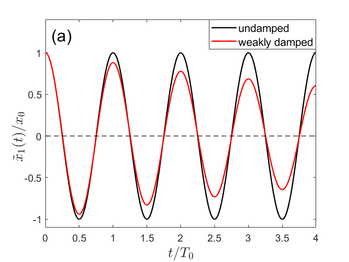
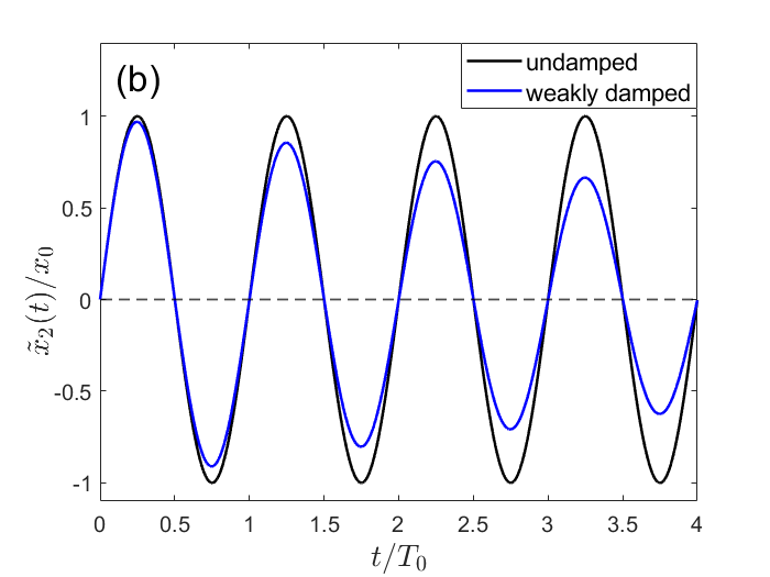
Figure 1: (a) The red curve shows the displacement $\tilde{x}_{1}(t)$ of weakly damped system (with some $m$, $k$ and $b$) for initial conditions $\tilde{x}_{1}(0)=x_{0}$ and $\tilde{v}_{1}(0)=0$. For comparison, the black curve shows the undamped solution with the same initial conditions, i.e., $x(t)=x_{0}\cos(\omega_{0}t)$. (b) The blue curve shows the displacement $\tilde{x}_{2}(t)$ of the same weakly damped system for initial conditions $\tilde{x}_{2}(0)=0$ and $\tilde{v}_{2}(0)=v_{0}=\omega_{0}x_{0}$, while the black curve shows the undamped solution with these initial conditions, i.e., $x(t)=x_{0}\sin(\omega_{0}t)$, for comparison. In both figures, the time is in $T_{0}=2\pi/\omega_{0}$ units, and the displacement is in $x_{0}$ units.

Let’s imagine that the instructor gives his students Fig. 1 with graphic representations of the exact solutions of equation (1) for a weakly damped system and an undamped system, for two pairs of initial conditions, which have the same initial energy $E_{0}$. One pair of initial conditions has a purely potential initial energy, while the other pair of initial conditions has a purely kinetic initial energy. The analytical expressions of the damped solutions used in Fig. 1 are given in section IV. Now comes the statement of the problem. The instructor says to the students: ”Find the expression for the energy decay of weakly damped system, using the insights provided by Fig. 1 and the energy dissipation rate (3). Furthermore, find what condition $b$ must satisfy, compared to $m$ and $k$, for the system to be weakly damped.”

III Modeling of the amplitude decrease and the energy decay of weakly damped harmonic oscillator

In Fig. 1(a) and (b), we see that the frequency and phase of $\tilde{x}_{1}(t)$ and $\tilde{x}_{2}(t)$ remain unchanged compared to the undamped solutions (at least as far as we can see from Fig. 1(a) and (b)), while the amplitudes of $\tilde{x}_{1}(t)$ and $\tilde{x}_{2}(t)$ slowly decrease with time in the same fashion. It is reasonable to describe the slow decay of the amplitudes of $\tilde{x}_{1}(t)$ and $\tilde{x}_{2}(t)$ with the same function, even though we can notice that the first few extremes of $\tilde{x}_{2}(t)$ are slightly smaller in magnitude than the extremes of $\tilde{x}_{1}(t)$ (for later times, the difference in the magnitude of extremes is hardly visible), since this can be explained by the fact that $\tilde{x}_{2}(t)$ reaches each extreme $T_{0}/4$ time later than $\tilde{x}_{1}(t)$, so $\tilde{x}_{2}(t)$ is exposed to damping for more extended time up to the moment of reaching the extremes compared to $\tilde{x}_{1}(t)$. These insights suggest that the weakly damped displacements shown in Fig. 1(a) and (b) can be modeled with

$$x_{1}(t)=f(t)x_{0}\cos(\omega_{0}t)\,$$ (4)

and

$$x_{2}(t)=f(t)x_{0}\sin(\omega_{0}t)\,$$ (5)

where function $f(t)$ describes the amplitude decrease in time. From (4) and (5) we calculate the corresponding velocities

$$v_{1}(t)=\frac{dx_{1}(t)}{dt}=-f(t)\omega_{0}x_{0}\sin(\omega_{0}t)+\dot{f}(t)x_{0}\cos(\omega_{0}t)$$ (6)

and

$$v_{2}(t)=\frac{dx_{2}(t)}{dt}=f(t)\omega_{0}x_{0}\cos(\omega_{0}t)+\dot{f}(t)x_{0}\sin(\omega_{0}t)\,,$$ (7)

where we used notation $\dot{f}(t)=df(t)/dt$. Since $\tilde{x}_{1}(0)=x_{0}$ and $\tilde{v}_{2}(0)=\omega_{0}x_{0}$ we can easily see that $f(0)=1$ must hold in order that our modeled solutions $x_{1}(t)$ and $x_{2}(t)$ satisfy these initial conditions. Furthermore, our modeled solution $x_{1}(t)$ has a initial velocity, i.e. $v_{1}(0)=\dot{f}(0)x_{0}$, while $\tilde{x}_{1}(t)$ has zero initial velocity. We deal with this issue in the following two paragraphs.

It is clear from Fig. 1(a) and (b) that the amplitudes of $\tilde{x}_{1}(t)$ and $\tilde{x}_{2}(t)$ change very slowly in time in comparison to the oscillating parts. Therefore, the rate of change of function $f(t)$ over time has to be much slower than the rate of change of $\cos(\omega_{0}t)$ and $\sin(\omega_{0}t)$, which is of the order $\omega_{0}$. We can conclude that $|\dot{f}(t)|\ll\omega_{0}$ holds for weak damping for all time, i.e., for $t\geq 0$ (we have put absolute value because we can expect the negative derivative of $f(t)$ since the amplitude decreases with time).

Regarding the discrepancy of our modeled solution $x_{1}(t)$, i.e., (4), and $\tilde{x}_{1}(t)$ in initial velocity, we can easily see that adding a phase $\phi$ to cosine in $x_{1}(t)$ could resolve this issue since it would lead to the initial velocity of the form

$$v_{1}(0)=-f(0)\omega_{0}x_{0}\sin(\phi)+\dot{f}(0)x_{0}\cos(\phi)$$ (8)

and, by setting $v_{1}(0)=0$, one easily gets that $\phi=\arctan(\dot{f}(0)/\omega_{0}))$ resolves this issue, but, due to the condition $|\dot{f}(0)|\ll\omega_{0}$, we can see that $\phi\ll 1$ holds. This leads us to the conclusion that $\tilde{x}_{1}(t)$ has a phase, but which is so small that it is unobservable in Fig. 1(a). Thus, adding this phase into our model would be an unnecessary complication, i.e., (4) is a valid model of $\tilde{x}_{1}(t)$.

By using our modeled displacements and velocities in (2), we get the corresponding energies

$$E_{1}(t)=E_{0}\left[f^{2}(t)-f(t)\left(\frac{\dot{f}(t)}{\omega_{0}}\right)\sin(2\omega_{0}t)+\left(\frac{\dot{f}(t)}{\omega_{0}}\right)^{2}\cos^{2}(\omega_{0}t)\right]$$ (9)

and

$$E_{2}(t)=E_{0}\left[f^{2}(t)+f(t)\left(\frac{\dot{f}(t)}{\omega_{0}}\right)\sin(2\omega_{0}t)+\left(\frac{\dot{f}(t)}{\omega_{0}}\right)^{2}\sin^{2}(\omega_{0}t)\right]\,,$$ (10)

where $E_{0}=m\omega_{0}^{2}x_{0}^{2}/2$ is the initial energy, and we used well know trigonometric identities $\sin^{2}(\omega_{0}t)+\cos^{2}(\omega_{0}t)=1$ and $\sin(2\omega_{0}t)=2\sin(\omega_{0}t)\cos(\omega_{0}t)$ in deriving (9) and (10). We can see that our modeled solution $x_{2}(t)$ has the right initial energy, i.e. $E_{2}(0)=E_{0}$, while $x_{1}(t)$ has initial energy $E_{1}(0)=E_{0}\left(1+(\dot{f}(0)/\omega_{0})^{2}\right)$. Since $|\dot{f}(t)|\ll\omega_{0}$ holds for weak damping, we can safely neglect the terms of the order $(\dot{f}(t)/\omega_{0})^{2}$ in (9) and (10). Thus, to the first order in $(\dot{f}(t)/\omega_{0})$, our modeled expressions for the energies are

$$E_{1}(t)=E_{0}\left[f^{2}(t)-f(t)\left(\frac{\dot{f}(t)}{\omega_{0}}\right)\sin(2\omega_{0}t)\right]$$ (11)

and

$$E_{2}(t)=E_{0}\left[f^{2}(t)+f(t)\left(\frac{\dot{f}(t)}{\omega_{0}}\right)\sin(2\omega_{0}t)\right]\,.$$ (12)

Both (11) and (12) have the correct initial energy. Now we focus on determining the $f(t)$.

If one would put, e.g., the energy (11) into the equation (3), i.e., $dE_{1}(t)/dt=-bv_{1}(t)^{2}$, it would lead to a very complicated differential equation for $f(t)$, but instead of that we can use the following trick. We add the dissipation rates corresponding to two pairs of initial conditions, i.e.

$$\frac{d}{dt}\left(E_{1}(t)+E_{2}(t)\right)=-b\left(v_{1}^{2}(t)+v_{2}^{2}(t)\right)\,.$$ (13)

Since $E_{1}(t)+E_{2}(t)=2E_{0}f(t)^{2}$, and $v_{1}^{2}(t)+v_{2}^{2}(t)=\omega_{0}^{2}x_{0}^{2}f^{2}(t)$ (in adding the squared velocities we again neglected the terms of the order $(\dot{f}(t)/\omega_{0})^{2}$) we get the differential equation

$$\frac{d}{dt}f^{2}(t)=-\frac{b}{m}f^{2}(t)\,.$$ (14)

Using substitutions $F(t)=f^{2}(t)$ and $\alpha=-b/m$, (14) becomes $dF(t)/dt=\alpha F(t)$, and first year undergraduates know that the function $F(t)=e^{\alpha t}$ satisfies this differential equation [3]. Thus, we obtain

$$f(t)=\sqrt{F(t)}=e^{-\frac{b}{2m}t}$$ (15)

as the slowly decaying amplitude of our modeled solutions (4) and (5). Using (15), and its time derivative, in (11) and (12) we get

$$E_{1}(t)=E_{0}e^{-\frac{b}{m}t}\left[1+\frac{b}{2m\omega_{0}}\sin(2\omega_{0}t)\right]$$ (16)

and

$$E_{2}(t)=E_{0}e^{-\frac{b}{m}t}\left[1-\frac{b}{2m\omega_{0}}\sin(2\omega_{0}t)\right]\,$$ (17)

as final expressions for the energies in our model.

We can now easily find what condition $b$ must satisfy, compared to $m$ and $k$, for the system to be weakly damped. As we stated before, for weak damping condition $|\dot{f}(t)|\ll\omega_{0}$ holds. This condition holds for all $t$, thus, if we consider $t=0$, for which $\dot{f}(0)=-b/(2m)$, we get

$$\frac{b}{2m}\ll\omega_{0}$$ (18)

as the condition of weak damping. Since $\omega_{0}=\sqrt{k/m}$, (18) can be rewritten as $b\ll 2\sqrt{mk}$, which is a common form of the weak damping condition in physics textbooks [3].

IV Comparison of our model with exact results

The exact solution of differential equation (1), for general initial conditions, is given, e.g., in [6]. For a pair of initial conditions, which we considered in Fig. 1(a) and (b), the exact solutions are

$$\tilde{x}_{1}(t)=\frac{\omega_{0}x_{0}}{\omega}e^{-\frac{b}{2m}t}\cos\left(\omega t-\arctan\left(\frac{b}{2m\omega}\right)\right)\,$$ (19)

and

$$\tilde{x}_{2}(t)=\frac{\omega_{0}x_{0}}{\omega}e^{-\frac{b}{2m}t}\sin\left(\omega t\right)\,$$ (20)

where $\omega=\sqrt{\omega_{0}^{2}-\left(\frac{b}{2m}\right)^{2}}$ is the damped angular frequency. In Fig. 1(a) and (b) we took $\frac{b}{2m}=0.02\omega_{0}$, which is in good agreement with weak damping condition (18). In this case, (19) and (20) become

$$\tilde{x}_{1}(t)=1.0002\,e^{-0.02\omega_{0}t}x_{0}\cos\left(0.9998\,\omega_{0}t-0.0020\right)\,$$ (21)

and

$$\tilde{x}_{1}(t)=1.0002\,e^{-0.02\omega_{0}t}x_{0}\sin\left(0.9998\,\omega_{0}t\right)\,,$$ (22)

where we rounded numbers to four decimals, thus, even without showing a graphical comparison, it is clear that our modeled solution (4) and (5), with $f(t)=e^{-0.02\omega_{0}t}$, approximate excellently the exact solutions (21) and (22). To further test the validity, but also to gain insight into the limits of our model, in Fig. 2 we show the modeled solutions (4) and (5) for $\frac{b}{2m}=0.1\omega_{0}$, and the corresponding exact solutions (19) and (20). We see only a slight mismatch between the modeled and the exact solutions. Thus, our model describes well the exact solutions (at least) for $0<\frac{b}{2m}\leq 0.1\omega_{0}$.

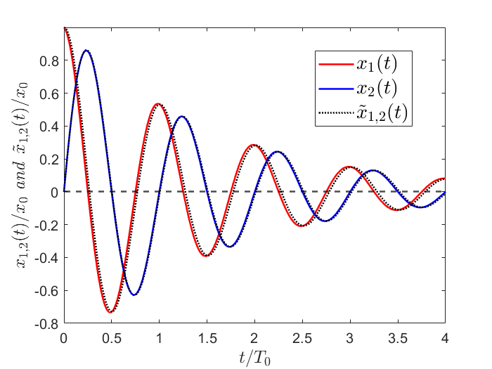
Figure 2: Modeled solutions $x_{1}(t)$ (red curve) and $x_{2}(t)$ (blue curve) given by (4) and (5) for $\frac{b}{2m}=0.1\omega_{0}$. The corresponding exact solutions $\tilde{x}_{1}(t)$ and $\tilde{x}_{2}(t)$ given by (19) and (20) are shown as dotted curves.

The exact expression for the energy of the damped harmonic oscillator, for general initial conditions, is given, e.g., in [7]. For a pair of initial conditions, which we considered in Fig. 1(a) and (b), the exact energies are

$$\tilde{E}_{1,2}(t)=E_{0}e^{-\frac{b}{m}t}\left[\cos^{2}(\omega t)\pm\frac{b}{2m\omega}\sin(2\omega t)+\frac{\omega_{0}^{2}+\left(\frac{b}{2m}\right)^{2}}{\omega^{2}}\sin^{2}(\omega t)\right]\,,$$ (23)

where the upper sign in $\pm$ corresponds to $\tilde{E}_{1}(t)$, and lower sign to $\tilde{E}_{2}(t)$. In Fig. 3 we show the modeled energies and the exact energies for $\frac{b}{2m}=\{0.02\omega_{0},0.05\omega_{0},0.1\omega_{0}\}$. We can see excellent agreement between our modeled energies and the exact energies.

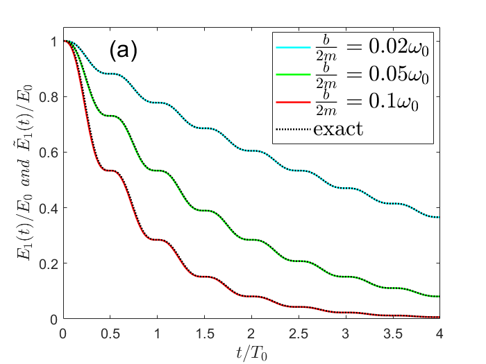
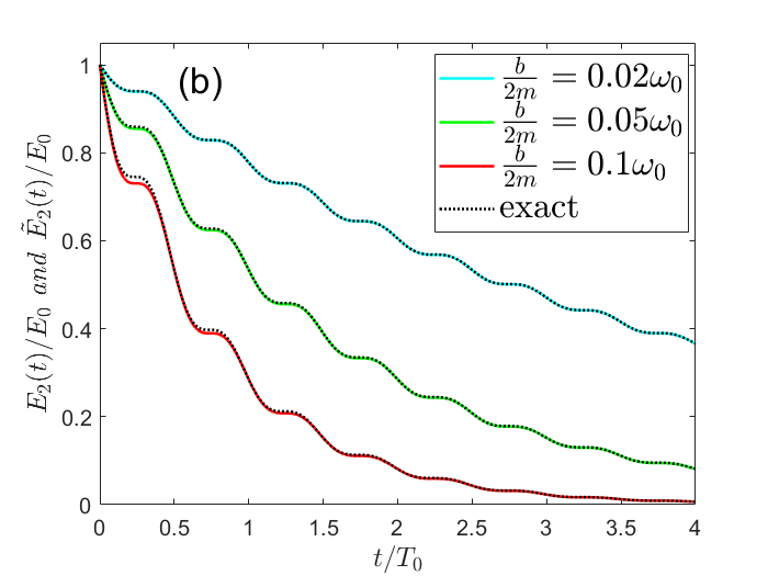
Figure 3: (a) Modeled energy $E_{1}(t)$, i.e. (16). (b) Modeled energy $E_{2}(t)$, i.e. (17). Both figures show the behavior for $\frac{b}{2m}=\{0.02\omega_{0},0.05\omega_{0},0.1\omega_{0}\}$. The corresponding exact energies $\tilde{E}_{1}(t)$ and $\tilde{E}_{2}(t)$, given by (23), are shown as dotted curves on both figures.

V A simpler version of our model

Exponential amplitude decay and purely exponential approximation of the energy decay of weakly damped harmonic oscillator have recently been derived using the energy dissipation rate averaged over one period of the corresponding undamped system, i.e. $T_{0}$, with the approximation that the amplitude remains constant over time intervals $\Delta t\sim T_{0}$ [8]. In our model, this approximation corresponds to neglecting terms with $\dot{f}(t)$ in the velocities (6) and (7), while the displacements (4) and (5) remain the same. In this case, it is easy to show that the modeled energies for both pairs of initial conditions are the same, i.e.

$$E_{1}(t)=E_{2}(t)=\frac{m\omega_{0}^{2}x_{0}^{2}}{2}f^{2}(t)\,,$$ (24)

and the corresponding dissipation rates are

$$\frac{dE_{1}(t)}{dt}=-bf^{2}(t)\omega_{0}^{2}x_{0}^{2}\sin^{2}(\omega_{0}t)\,$$ (25)

and

$$\frac{dE_{2}(t)}{dt}=-bf^{2}(t)\omega_{0}^{2}x_{0}^{2}\cos^{2}(\omega_{0}t)\,.$$ (26)

Now, it is even easier to see that the sum of (25) and (26) leads to equation (14). Thus, we obtain $f(t)=e^{-\frac{b}{2m}t}$ again, but in this case, we only get the exponential energy decay, i.e., $E_{1}(t)=E_{2}(t)=E_{0}e^{-\frac{b}{m}t}$, which is a good approximation of the exact energies (23), with $\frac{b}{2m}\ll\omega_{0}$, only if one is interested in behavior of the energy on time scales greater than $T_{0}$. This simplified version of our derivation is suitable for high school students, i.e., from a mathematical point of view, it is at a slightly lower level of difficulty than the method presented in [8] since there is no need to calculate the time integral of the energy dissipation rate if our trick is used.

VI Conclusion

We showed how to obtain an excellent approximation of the solutions and the energy of a weakly damped harmonic oscillator without solving the differential equation of the second order, i.e., equation (1), and without any previous insights into the analytical form of the solutions of that equation. The model we introduced and the trick we used are suitable for first-year undergraduates. In addition, we commented on a simplified version of our model and derivation, which are more suitable for high school students.

VII Acknowledgments

This work was supported by the QuantiXLie Center of Excellence, a project co-financed by the Croatian Government and European Union through the European Regional Development Fund, the Competitiveness and Cohesion Operational Programme (Grant No. KK.01.1.1.01.0004).

References

- [1] J.D. Cutnell and K.W. Johnson. Physics. John Wiley & Sons, 2009.
- [2] David Halliday, Robert Resnick, and Jearl Walker. Fundamentals of Physics. John Wiley & Sons, 2013.
- [3] Hugh D. Young and Roger A. Freedman. University Physics with Modern Physics. Pearson, 2020.
- [4] Peter F. Hinrichsen. Acceleration, Velocity, and Displacement for Magnetically Damped Oscillations. The Physics Teacher, 57(4):250–253, 04 2019.
- [5] Manuel I González and Alfredo Bol. Controlled damping of a physical pendulum: experiments near critical conditions. European Journal of Physics, 27(2):257, jan 2006.
- [6] Karlo Lelas, Nikola Poljak, and Dario Jukić. Damped harmonic oscillator revisited: The fastest route to equilibrium. American Journal of Physics, 91(10):767–775, 10 2023.
- [7] K. Lelas and I. Nakić. Optimal damping of vibrating systems: Dependence on initial conditions. Journal of Sound and Vibration, 576:118303, 2024.
- [8] Stylianos-Vasileios Kontomaris and Anna Malamou. An elementary proof of the amplitude’s exponential decrease in damped oscillations. Physics Education, 59(2):025030, feb 2024.