Bayesian inverse Navier–Stokes problems:
joint flow field reconstruction and parameter learning

Abstract

We formulate and solve a Bayesian inverse Navier–Stokes (N–S) problem that assimilates velocimetry data in order to jointly reconstruct a 3D flow field and learn the unknown N–S parameters, including the boundary position. By hardwiring a generalised N–S problem, and regularising its unknown parameters using Gaussian prior distributions, we learn the most likely parameters in a collapsed search space. The most likely flow field reconstruction is then the N–S solution that corresponds to the learned parameters. We develop the method in the variational setting and use a stabilised Nitsche weak form of the N–S problem that permits the control of all N–S parameters. To regularise the inferred the geometry, we use a viscous signed distance field (vSDF) as an auxiliary variable, which is given as the solution of a viscous Eikonal boundary value problem. We devise an algorithm that solves this inverse problem, and numerically implement it using an adjoint-consistent stabilised cut-cell finite element method. We then use this method to reconstruct magnetic resonance velocimetry (flow-MRI) data of a 3D steady laminar flow through a physical model of an aortic arch for two different Reynolds numbers and signal-to-noise ratio (SNR) levels (low/high). We find that the method can accurately i) reconstruct the low SNR data by filtering out the noise/artefacts and recovering flow features that are obscured by noise, and ii) reproduce the high SNR data without overfitting. Although the framework that we develop applies to 3D steady laminar flows in complex geometries, it readily extends to time-dependent laminar and Reynolds-averaged turbulent flows, as well as non-Newtonian (e.g. viscoelastic) fluids.

1 Introduction

For inverse problems in flow field imaging (velocimetry), a priori knowledge takes the form of a Navier–Stokes (N–S) problem. The problem of reconstructing and segmenting a flow image can then be expressed as a generalised inverse Navier–Stokes problem whose flow domain, boundary conditions, and model parameters have to be inferred in order for the modelled velocity (i.e. the reconstruction) to approximate the measured velocity in an appropriate metric space. This approach not only produces a reconstruction that can be made to be an accurate fluid flow inside or around the object, but also provides additional physical knowledge (e.g. pressure, wall shear stress, and effective viscosity field/tensor), which is otherwise difficult or impossible to measure. Inverse N–S problems have been intensively studied during the last decade, mainly enabled by the increase of available computing power. Recent applications in fluid dynamics range from the forcing inference problem [Fou+14, HLS14], to the reconstruction of scalar image velocimetry (SIV) [Gil+18, Sha+19] and particle image velocimetry (PIV) [GBY19] data, and the identification of optimal sensor arrangements [MCS17, Ver+19]. Regularisation methods that can be used to reduce the search space of model parameters are reviewed in [Stu10] from a Bayesian perspective, and in [BB18] from a variational perspective. The well-posedness of Bayesian inverse N–S problems has been addressed in [Cot+09].

1.1 Flow field reconstruction

In [KB18] the authors treat the reduced inverse N–S problem of finding the Dirichlet boundary condition for the inlet velocity that matches the modelled velocity field to flow-MRI data for a steady 3D flow in a glass replica of the human aorta. They measure the model-data discrepancy using the $L^{2}$-norm and introduce additional variational regularisation terms for the Dirichlet boundary condition. The same formulation is extended to periodic flows in [Kol19, KCH19], using the harmonic balance method for the temporal discretisation of the N–S problem. In [Fun+19] the authors address the problem of inferring both the inlet velocity (Dirichlet) boundary condition and the initial condition, for unsteady blood flows and 4D flow-MRI data in a cerebral aneurysm. Note that the above studies consider rigid boundaries and require a priori an accurate, and time-averaged, geometric representation of the blood vessel, which is a severe constraint on the inverse problem of finding the velocity field.

To find the shape of the flow domain, e.g. the blood vessel boundaries, computed tomography (CT) or magnetic resonance angiography (MRA) is often used. The acquired image is then reconstructed, segmented, and smoothed. This process not only requires substantial effort and the design of an additional experiment (e.g. CT, MRA), but it also introduces geometric uncertainties [Mor+16, San+16], which, in turn, affect the predictive confidence of arterial wall shear stress distributions and their mappings [Kat+07, Sot+16]. For example, in [Fun+19] the authors report discrepancies between the modelled and the measured velocity fields near the flow boundaries, and they suspect they are caused by geometric errors that were introduced during the boundary segmentation process. In general, the assumption of rigid boundaries either implies that a time-averaged geometry has to be used, or that an additional experiment (e.g. CT, MRA) has to be conducted to register the moving boundaries to the flow measurements. A more consistent approach to this problem is to treat the blood vessel geometry as an unknown when solving the generalised inverse N–S problem [Kon+22]. In this way, the method simultaneously reconstructs and segments the velocity fields and can better adapt to the velocimetry experiment by correcting the geometric errors and improving the reconstruction. In other words, the velocity field is used to find the boundary, and the boundary is used to find the velocity field. This is a neater optimisation problem since it removes the severe constraint of fixing the boundary before assimilating the velocity field.

In this study we build upon the work in [Kon+22]. In particular, we extend the methodology from 2D to 3D flows, revise and improve the implicit representation of the geometry by incorporating the viscous Eikonal equation as an additional constraint to the problem, and design an adjoint-consistent discrete formulation (i.e. the discretised continuous adjoint operator is equivalent to the discrete adjoint operator). We then devise an algorithm that solves this Bayesian inverse N–S problem, and demonstrate it on flow-MRI data of a 3D steady laminar flow through a physical model of an aortic arch.

1.1.1 Deep learning reconstruction algorithms

Artificial intelligence (AI) algorithms, such as deep neural networks (NNs), are versatile, relatively simpler to implement, and have revolutionised the field of computer vision. There are, however, fundamental problems that still need to be addressed for their application to physics-based problems such as flow field reconstruction (e.g. AI-generated hallucinations, and the problem of existence of stable computational algorithms) [Muc+21, CAH22]. Physics-informed NNs (PINNs) cannot yet solve boundary value problems, (e.g the N–S problem) more efficiently than finite element methods [Gro+23]. Further, PINNs contain orders of magnitude more degrees of freedom than the method in this paper, with a corresponding increase in the required amounts of data and training time. The method in this paper is, in contrast, formulated from a N–S boundary value problem in a variational framework. The physics is hardwired into the model, meaning that the search space is restricted to solutions that satisfy the N–S problem. This is a key-difference between PINNs and the approach in this study: while PINNs solve a minimisation problem, we solve a saddle point problem. In other words, PINNs do not hardwire the N–S problem; they simply penalise its residuals (i.e. they treat the N–S problem as a soft constraint). In our experience, solving the saddle point problem, even though more computationally expensive, leads to superior flow field reconstructions and more accurate inferred parameters. Unlike NNs [Fer+20, RRAJ21] and PINNs [Sai+24, Zhu+24], our model is relatively small, physically interpretable, amenable to mathematical analysis, extrapolatable, and will reconstruct flows that it has not seen before, thus enabling digital twin applications in engineering design and patient-specific cardiovascular modelling.

1.2 Outline

• In section 2 we present the general framework for the Bayesian inversion of nonlinear models.

• In section 3 we formulate the Bayesian inversion of the Navier–Stokes problem, in a continuous, variational setting, and devise an algorithm that solves it.

• In section 4 we formulate the discrete Bayesian inverse N–S problem, and discuss the details of its numerical implementation.

• In section 5 we use the algorithm to reconstruct flow-MRI data of a 3D steady laminar flow through a physical model of an aortic arch.

1.3 Notation

In what follows, $L^{2}(\Omega)$ denotes the space of square-integrable functions in $\Omega$, with inner product $\big{\langle}\cdot,\cdot\big{\rangle}$ and norm $\lVert\cdot\rVert_{L^{2}(\Omega)}$, and $H^{k}(\Omega)$ denotes the space of square-integrable functions with $k$ square-integrable derivatives. For a given covariance operator, $\mathcal{C}$, we also define the covariance-weighted $L^{2}(\Omega)$ spaces, endowed with the inner product ${\big{\langle}\cdot,\cdot\big{\rangle}_{\mathcal{C}(\Omega)}:=\big{\langle}\mathcal{C}^{-1/2}\cdot,\mathcal{C}^{-1/2}\cdot\big{\rangle}}_{\Omega}$, which generates the norm $\lVert\cdot\rVert_{\mathcal{C}(\Omega)}$ (or the semi-norm $|{\cdot}|_{\mathcal{C}(\Omega)}$ if $\mathcal{C}^{-1}$ has a non-trivial kernel). The Euclidean norm in the space of real numbers $\mathbb{R}^{n}$ is denoted by $\lvert\cdot\rvert_{\mathbb{R}^{n}}$, and the measure (volume) of the domain $\Omega$ by $\lvert\Omega\rvert$. The first variation of a functional $\mathscr{J}:L^{2}\to\mathbb{R}$ is defined by

$$\delta_{z}\mathscr{J}\equiv\frac{d}{d\tau}\mathscr{J}({z}+\tau{z}^{\prime})\Big{|}_{\tau=0}=\big{\langle}D_{z}\mathscr{J},z^{\prime}\big{\rangle}\quad,$$ (1)

where $\tau\in\mathbb{R}$, $z\in L^{2}$, $z^{\prime}\in L^{2}$ is an allowed perturbation of $z$, and $D_{z}\mathscr{J}$ is the generalised gradient. We use the superscript $(\cdot)^{*}$ to denote the adjoint of an operator, $(\cdot)^{\star}$ to denote a measurement, and $(\cdot)^{\circ}$ to denote a reconstruction. For instance, $\bm{u}^{\star}$ denotes the measured velocity obtained from a velocimetry experiment, $\bm{u}^{\circ}$ denotes the corresponding reconstructed velocity field, and $\bm{u}$ denotes a (modelled) velocity field obtained from the N–S problem.

2 Bayesian inversion of nonlinear models

Given experimental, possibly noisy and sparse, vector field data of a physical quantity, $\bm{u}^{\star}$, we assume that we already know a physical model, $\bm{u}=\bm{u}(\bm{x})$, that can fit the data for suitable, physically-interpretable parameters, $\bm{x}$. In other words, there exist parameters $\bm{x}^{\circ}$ such that

$$\bm{u}^{\star}\simeq\mathcal{Z}\bm{x}^{\circ}=\big{(}\mathcal{S}\mathcal{Q}\big{)}\bm{x}^{\circ}=\mathcal{S}\bm{u}^{\circ}\quad,$$ (2)

where $\mathcal{Z}\coloneqq\mathcal{S}\mathcal{Q}$ is the operator that maps model parameters to model solutions projected into the data space, $\mathcal{S}$ is the model space to data space projection operator, which is linear and non-invertible, and $\mathcal{Q}$ is the operator that encapsulates the physical model, which is nonlinear and invertible. Under this assumption, the main goal is to find $\bm{x}^{\circ}$, which is of interest because it often pertains to physical quantities that cannot be directly measured, and which are instead inferred from the data. At the same time, we obtain the reconstructed (model-filtered) velocity field, $\bm{u}^{\circ}\equiv\mathcal{Q}\bm{x}^{\circ}$, which fits the noisy, sparse, and under-resolved data. Starting from the assumptions that i) the model explains the data, and ii) the data noise is Gaussian, we write

$$\bm{u}^{\star}-\mathcal{Z}\bm{x}=\bm{\varepsilon}\sim\mathcal{N}(\bm{0},\mathcal{C}_{\bm{u}^{\star}})\quad,$$ (3)

where $\bm{\varepsilon}\sim\mathcal{N}(\bm{0},\mathcal{C}_{\bm{u}^{\star}})$ is Gaussian noise with zero mean and with covariance operator $\mathcal{C}_{\bm{u}^{\star}}$. We also assume that we have prior knowledge of the probability distribution of the model parameters, $\bm{x}$. We call this the prior parameter distribution, $\mathcal{N}(\bar{\bm{x}},\mathcal{C}_{\bar{\bm{x}}})$, which we assume to be Gaussian with prior mean $\bar{\bm{x}}$, and prior covariance operator $\mathcal{C}_{\bar{\bm{x}}}$. We then use Bayes’ theorem, which states that the posterior probability density function (p.d.f.) of $\bm{x}$, given the data $\bm{u}^{\star}$, $\pi\big{(}\bm{x}\big{|}\bm{u}^{\star}\big{)}$, is proportional to the data likelihood, $\pi\big{(}\bm{u}^{\star}\big{|}\bm{x}\big{)}$, times the prior p.d.f. of $\bm{x}$, $\pi\big{(}\bm{x}\big{)}$, i.e.

$$\pi\big{(}\bm{x}\big{|}\bm{u}^{\star}\big{)} \propto\pi\big{(}\bm{u}^{\star}\big{|}\bm{x}\big{)}~{}\pi(\bm{x})$$

$$=\exp\Big{(}-\frac{1}{2}\lVert\bm{u}^{\star}-\mathcal{Z}\bm{x}\rVert^{2}_{\mathcal{C}_{\bm{u}^{\star}}}-\frac{1}{2}\lVert\bm{x}-\bar{\bm{x}}\rVert^{2}_{\mathcal{C}_{\bar{\bm{x}}}}\Big{)}$$ (4)

where $\pi(\cdot)$ is the Gaussian p.d.f., and $\lVert\cdot,\cdot\rVert^{2}_{\mathcal{C}}\coloneqq\big{\langle}\cdot,\mathcal{C}^{-1}\cdot\big{\rangle}$ is the covariance-weighted $L^{2}$-norm. The most likely parameters $\bm{x}^{\circ}$, in the sense that they maximise the posterior p.d.f. (maximum a posteriori probability, or MAP estimator), are given implicitly as the solution of the nonlinear optimisation problem

$$\quad\bm{x}^{\circ}\equiv\underset{\bm{x}}{\mathrm{argmin}}\mathscr{J}(\bm{x})\quad,\quad\text{where}\quad\mathscr{J}\coloneqq-\log\pi\big{(}\bm{x}\big{|}\bm{u}^{\star}\big{)}\quad.$$ (5)

2.1 Nonlinearity and optimisation

In order to solve problem (5) we first linearise $\mathcal{Q}$ around $\bm{x}_{k}$, i.e.

$$\bm{u}=\mathcal{Q}\bm{x}\simeq\mathcal{Q}\bm{x}_{k}+\mathcal{A}_{k}\big{(}\bm{x}-\bm{x}_{k})\quad,$$ (6)

where $\mathcal{A}_{k}\equiv\big{(}D^{\bm{u}}_{\bm{x}}\big{)}_{k}$ is the Jacobian of $\bm{u}$ with respect to $\bm{x}$. In the same spirit, we obtain

$$\mathcal{Z}\bm{x}\simeq\mathcal{Z}\bm{x}_{k}+\mathcal{G}_{k}\big{(}\bm{x}-\bm{x}_{k})\quad,\quad\mathcal{G}_{k}\coloneqq\mathcal{S}\mathcal{A}_{k}\quad.$$ (7)

The first order optimality conditions of problem (5) then lead to the following update rule [Tar05]

$$\bm{x}_{k+1}\mathrel{\reflectbox{$\mapsto$}}\bm{x}_{k}+\tau_{k}~{}\mathcal{C}_{\bm{x}_{k}}~{}\big{(}D_{\bm{x}}\mathscr{J}\big{)}_{k}\quad,$$ (8)

where $\tau_{k}$ is the step size at iteration $k$, which is determined by a line search algorithm, $\mathcal{C}_{\bm{x}_{k}}$ is the posterior (parameter) covariance operator at iteration $k$, which is given by

$$\mathcal{C}_{\bm{x}_{k}}\coloneqq\big{(}\mathcal{G}_{k}^{*}~{}\mathcal{C}_{\bm{u}^{\star}}^{-1}~{}\mathcal{G}_{k}+\mathcal{C}_{\bar{\bm{x}}}^{-1}\big{)}^{-1}\quad,$$ (9)

where $\mathcal{G}^{*}_{k}$ is the adjoint of $\mathcal{G}_{k}$, and $\big{(}D_{\bm{x}}\mathscr{J}\big{)}_{k}$ is the gradient of the objective, $\mathscr{J}$, with respect to the parameters, $\bm{x}$, which is given by

$$\big{(}D_{\bm{x}}\mathscr{J}\big{)}_{k}\coloneqq\underbrace{\mathcal{G}_{k}^{*}~{}\mathcal{C}_{\bm{u}^{\star}}^{-1}\big{(}\bm{u}^{\star}-\mathcal{Z}\bm{x}_{k}\big{)}}_{\text{model term}}+\underbrace{\mathcal{C}_{\bar{\bm{x}}}^{-1}\big{(}\bm{x}_{k}-\bar{\bm{x}}\big{)}}_{\text{prior term}}\quad.$$ (10)

2.2 Posterior distribution and the Gaussian assumption

For $\bm{x}$ in a neighbourhood of the MAP point, $\bm{x}^{\circ}$, we can furthermore write

$$\pi\big{(}\bm{x}\big{|}\bm{u}^{\star}\big{)}\simeq\widetilde{\pi}\big{(}\bm{x}\big{|}\bm{u}^{\star}\big{)}\coloneqq\exp\Big{(}-\frac{1}{2}\lVert\bm{x}-\bm{x}^{\circ}\rVert^{2}_{\mathcal{C}_{\bm{x}^{\circ}}}-\textrm{const.}\Big{)}\quad,$$ (11)

which is known as the Laplace approximation [Mac03, Chapter 27], and is exact when $\mathcal{Z}$ is a linear operator. Figure 1 illustrates the conceptual difference between linear, weakly nonlinear, and strongly nonlinear operators $\mathcal{Z}$. In this study, $\mathcal{Z}$ encodes a Navier–Stokes problem, and the ‘strength’ of the nonlinearity depends on the flow conditions (e.g. on the geometry and the boundary conditions) and the Reynolds number, $\mathit{Re}$. Note that, for $\mathit{Re}\ll 1$, the N–S problem can be approximated well enough by the Stokes problem, which is linear. At the other end of the spectrum, for sufficiently large $\mathit{Re}$, the flow becomes turbulent, which is a strongly nonlinear phenomenon. It should be emphasised that what matters is the behaviour of $\mathcal{Z}$ around the MAP point, $\bm{x}^{\circ}$, and within the $\sim 3\sigma$ support of the joint density, $\pi(\bm{x},\bm{u}^{\star})$. If $\mathcal{Z}$ is to be linearised around $\bm{x}^{\circ}$, the greater the spread of $\pi(\bm{x},\bm{u}^{\star})$, the less accurate the approximation will be. Also, the spread of $\pi(\bm{x},\bm{u}^{\star})$ depends on i) the noise level in the data, and ii) the assumed prior distribution of the N–S unknowns, $\bm{x}$. This implies that, when $\mathcal{Z}$ is strongly nonlinear, we may require higher-quality data and/or more informative priors in order to regularise the inverse problem. Alternatively, we can simplify or reformulate the model such that $\mathcal{Z}$ exhibits smoother behaviour. In turbulent flows, for example, the large scales will depend on the geometry and the boundary conditions of the problem, while the small scales of turbulence exhibit a universal behaviour that is not directly linked to these parameters. Hence, inferring the evolution of the averaged velocity and pressure fields using the Reynolds-averaged Navier–Stokes (RANS) equations, instead of the instantaneous fields that are governed by the N–S equations, can lead to a well-posed inverse problem. In this paper, however, we only consider laminar flow with a Newtonian viscosity model.

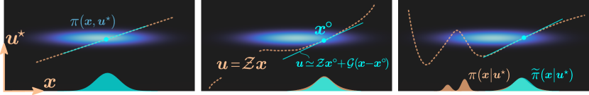
Figure 1: When $\mathcal{Z}$ is linear (left), $\pi(\bm{x}|\bm{u}^{\star})$ is Gaussian. When $\mathcal{Z}$ is weakly nonlinear (middle), $\pi(\bm{x}|\bm{u}^{\star})$ can be approximated reasonably well by a Gaussian p.d.f., $\widetilde{\pi}(\bm{x}|\bm{u}^{\star})$, around $\bm{x}^{\circ}$ (Laplace approximation). When $\mathcal{Z}$ is strongly nonlinear (right), $\pi(\bm{x}|\bm{u}^{\star})$ can even be multimodal, in which case there are multiple critical points which will yield different approximations $\widetilde{\pi}(\bm{x}|\bm{u}^{\star})$ (even locally, the approximation may be inaccurate).

2.3 Posterior covariance approximation

Instead of using formula (9) to compute the exact posterior parameter covariance operator, $\mathcal{C}_{\bm{x}_{k}}$, which is computationally expensive, we can approximate it using a quasi-Newton method (e.g. BFGS) [Fle00]. Quasi-Newton methods use the states, $\bm{x}_{k}$, and the gradients, $\big{(}D_{\bm{x}}\mathscr{J}\big{)}_{k}$, to reconstruct the Hessian operator or its inverse. In the case of the quadratic problem (5), the inverse Hessian operator, $H_{k}$, is identical to $\mathcal{C}_{\bm{x}_{k}}$. To derive the matrix-free (large-scale optimisation) BFGS formula [YJH96][Tar05, Chapter 6.22.8] for the inverse Hessian operator, we first set

$$\bm{s}_{k}\mathrel{\reflectbox{$\mapsto$}}\bm{x}_{k}-\bm{x}_{k-1}\quad\text{and}\quad\bm{y}_{k}\mathrel{\reflectbox{$\mapsto$}}\big{(}D_{\bm{x}}\mathscr{J}\big{)}_{k}-\big{(}D_{\bm{x}}\mathscr{J}\big{)}_{k-1}\quad.$$ (12)

The reconstructed inverse Hessian, $\widetilde{H}_{k}$, which is equivalent to the reconstructed posterior (parameter) covariance, $\widetilde{\mathcal{C}}_{k}$, is then given by the recursive formula

$$\widetilde{\mathcal{C}}_{k}~{}\square=\mathcal{C}_{\bar{\bm{x}}}~{}\square +\sum_{j=1}^{k-1}\big{(}1+\omega_{j}\rho_{j}\big{)}\rho_{j}~{}\big{\langle}\bm{s}_{j},\square\big{\rangle}~{}\bm{s}_{j}$$

$$+\sum_{j=1}^{k-1}-\rho_{j}~{}\big{\langle}\square,\bm{\alpha}_{j}\big{\rangle}~{}\bm{s}_{j}-\rho_{j}~{}\big{\langle}\bm{s}_{j},\square\big{\rangle}~{}\bm{\alpha}_{j}\quad,$$ (13)

where $\square$ is a placeholder for the argument, and $\omega_{j}\equiv\big{\langle}\bm{y}_{j},\widetilde{\mathcal{C}}_{j}\bm{y}_{j}\big{\rangle}$, $\rho_{j}\equiv 1/\big{\langle}\bm{y}_{j},\bm{s}_{j}\big{\rangle}$, and $\bm{\alpha}_{j}\equiv\widetilde{\mathcal{C}}_{j}\bm{y}_{j}$, are quantities that are computed only once and stored in memory. Note that we here choose to initialise the posterior covariance using the prior covariance, i.e. $\mathcal{C}_{0}\mathrel{\reflectbox{$\mapsto$}}\mathcal{C}_{\bar{\bm{x}}}$, but the best initialisation strategy depends on the specifics of the problem.

2.3.1 Uncertainty estimation

To estimate the predicted uncertainty around the MAP solution, we can use Arnoldi iteration to compute the eigendecomposition of either the exact posterior covariance, which is given by (9), or the approximated posterior covariance, which is given by (13). A third option is to reconstruct $\mathcal{C}_{\bm{x}^{\circ}}$ using the eigendecompositions of $\mathcal{G}_{\bm{x}^{\circ}}$, $\mathcal{G}^{*}_{\bm{x}^{\circ}}$, $\mathcal{C}_{\bm{u}^{\star}}^{-1}$, $\mathcal{C}_{\bar{\bm{x}}}^{-1}$, which may be simpler to compute. Once the eigenvalue/eigenvector pairs, $(\lambda,\bm{v})_{\ell}$, of the covariance operator are obtained, we find

$$\mathcal{C}_{\bm{x}^{\circ}}=\sum^{\infty}_{\ell}\lambda_{\ell}~{}\bm{v}_{\ell}\otimes\bm{v}_{\ell}\quad.$$ (14)

The pointwise variance, $\textrm{var}(\bm{x})$, which is often used to quantify uncertainty, is then given by

$$\mathrm{var}(\bm{x})=\sum^{\infty}_{\ell}\lambda_{\ell}~{}\bm{v}^{2}_{\ell}\quad,$$ (15)

and the total variance is given by

$$\lVert\bm{x}-\bm{x}^{\circ}\rVert^{2}_{\mathcal{C}_{\bm{x}^{\circ}}}=\sum^{\infty}_{\ell}\lambda_{\ell}\quad.$$ (16)

Samples, $\bm{x}^{s}$, can be drawn using the Karhunen–Loève (K–L) expansion

$$\bm{x}^{s}=\bm{x}^{\circ}+\sum^{\infty}_{\ell}\eta_{\ell}~{}\sqrt{\lambda_{\ell}}~{}\bm{v}_{\ell}\quad,\quad\text{with}\quad\mathbb{R}\ni\eta_{\ell}\sim\mathcal{N}(0,1)\quad,$$ (17)

in order to further inspect the posterior distribution around the MAP point. Likewise, the posterior covariance of the model solution at iteration $k$, which is given by

$$\mathcal{C}_{\bm{u}_{k}}\coloneqq\mathcal{A}_{\bm{x}_{k}}{\mathcal{C}}_{\bm{x}_{k}}\mathcal{A}_{\bm{x}_{k}}^{*}\quad,$$ (18)

can be reconstructed from the eigendecompositions of $\mathcal{C}_{\bm{x}_{k}}$, $\mathcal{A}_{k}$, and $\mathcal{A}^{*}_{k}$.

3 Bayesian inversion of the Navier–Stokes problem

In section 2 we discussed the general Bayesian inversion problem and the MAP estimator, given by (5), which can be iteratively solved by using the update rule (8) along with the objective gradients (10) and the posterior covariance (9) (or its BFGS-approximation) when the operators $\mathcal{C}_{\bm{u}^{\star}}$, $\mathcal{C}_{\bar{\bm{x}}}$, $\mathcal{S}$, $\mathcal{G}$, and $\mathcal{Q}$ are precisely defined. In order to obtain these operators for the Bayesian inversion of the generalised Navier–Stokes problem, we need to derive the first order optimality conditions of the following saddle point problem

$$\text{find}\quad\bm{x}^{\circ}\equiv\mathrm{arg}\ \underset{\bm{x}}{\mathrm{min}}\ \underset{\bm{v},q,r}{\mathrm{max}}~{}\mathscr{J}(\bm{u},p,\bm{v},q,r;\bm{x})\quad,$$ (19)

where

$${\mathscr{J}}(\bm{u},p,\bm{v},q,r;\bm{x})={\mathscr{U}}(\bm{u})+{\mathscr{M}}(\bm{u},p,\bm{v},q;\bm{x})+\mathscr{D}(r,\varphi_{\pm})+\mathscr{R}_{\bm{x}}(\bm{x})\quad.$$ (20)

The augmented objective functional, $\mathscr{J}$, incorporates the model-data discrepancy, $\mathscr{U}$, the generalised Navier–Stokes boundary value problem, $\mathscr{M}$, the viscous signed distance field (vSDF) boundary value problem, $\mathscr{D}$, and the priors of the N–S parameters, $\mathscr{R}_{\bm{x}}$. The vSDF, ${\varphi_{\pm}}$, is an auxiliary variable that we use to implicitly define and control the geometry. The Lagrange multipliers, $(\bm{v},q,r)$, also known as adjoint variables, are used to enforce the two model constraints: i) $(\bm{v},q)$ enforce the N–S b.v.p. for $(\bm{u},p)$, and ii) $r$ enforces the vSDF b.v.p. for ${\varphi_{\pm}}$. In this section, we first define $\mathcal{C}_{\bm{u}^{\star}}$ and $\mathcal{S}$, then we use variational calculus to construct $\mathcal{G}$ and $\mathcal{Q}$, and lastly we define $\mathcal{C}_{\bar{\bm{x}}}$. We further devise an algorithm that solves the Bayesian inverse N–S problem, which is presented at the end of this section.

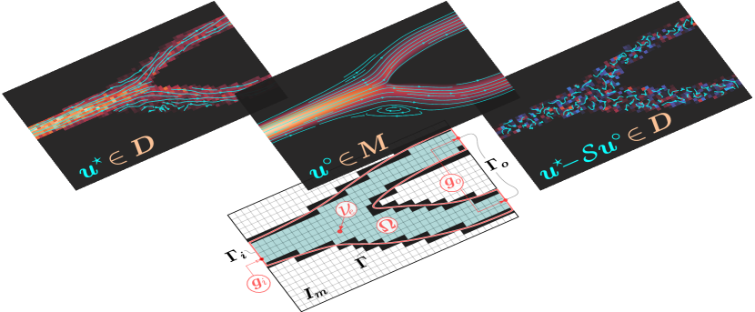
Figure 2: The Bayesian inverse N–S problem assimilates velocimetry data, $\bm{u}^{\star}$, in order to jointly reconstruct the flow field, $\bm{u}$, and learn the unknown N–S parameters, $\bm{x}$. The MAP estimator of the unknown N–S parameters, $\bm{x}^{\circ}$, is found by solving problem (19), and the reconstructed velocity field is given by $\bm{u}^{\circ}=\mathcal{Q}\bm{x}^{\circ}$.

3.1 Data-model discrepancy: operators $\mathcal{S}$, $\mathcal{C}_{\bm{u}^{\star}}$

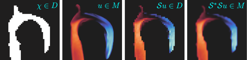
Figure 3: The projection operator $\mathcal{S}:\bm{M}\to\bm{D}$ is used to project the modelled velocity field, $\bm{u}\in\bm{M}$, to $\mathcal{S}\bm{u}\in\bm{D}$, so that it can be compared with the velocity data, $\bm{u}^{\star}$. A mask, $\chi$, is commonly used after pre-processing the data to remove irregularities such as outliers (e.g. defective pixels), or regions with no signal. The adjoint operator $\mathcal{S}^{*}$ is used to project from $\bm{D}$ to $\bm{M}$ (the inverse of $\mathcal{S}$ does not exist).

We define the data space $\bm{D}\equiv\bm{L}^{2}(I_{d})$, and the model space $\bm{M}\equiv\bm{L}^{2}(I_{m})$, where $I_{d}$, $I_{m}$ are bounded subsets of $\mathbb{R}^{3}$. The size of $I_{d}$ depends on the field of view (FOV) of the experiment, and the size of $I_{m}$ depends on the field of view of the model. For problems in velocity imaging, such as flow-MRI, the data domain, $I_{d}$, is a uniform tessellation consisting of $N$ (disjoint) voxels (or pixels in 2D), $\{V_{i}\}_{i=1}^{N}$, such that

$$I_{d}=\bigcup_{i=1}^{N}V_{i}\quad,\quad\text{and}\quad V_{i}\cap V_{j}=\varnothing\quad\text{for}~{}i\neq j\quad.$$ (21)

The data space, $\bm{D}$, is the function space on $I_{d}$ that is comprised of all piecewise constant functions

$$\bm{u}_{d}(x)=\sum_{i=1}^{N}\bm{\varphi}_{i}(x)~{}{\bm{u}^{i}_{d}}\quad,$$ (22)

where $\bm{\varphi}_{i}(x)\equiv(1,1,1)$ for $x\in V_{i}$ and $\bm{\varphi}_{i}(x)\equiv\bm{0}$ otherwise, and $\bm{u}^{i}_{d}\in\mathbb{R}^{3}$. In general, the model space, $\bm{M}$, is a subspace of $\bm{L}^{2}(I_{m})$, but more can be said about $\bm{M}$ and $I_{m}$ after discretising the N–S problem, which we will address in section 4.1. The data-model discrepancy is measured on the data space, and is given by

$$\mathscr{U}(\bm{u})\coloneqq\frac{1}{2}~{}\big{\lVert}\bm{u}^{\star}-\mathcal{S}\bm{u}\big{\rVert}^{2}_{{\mathcal{C}_{\bm{u}^{\star}}}}\quad,$$ (23)

where $\bm{u}=(u_{x},u_{y},u_{z})$, $\bm{u}^{\star}=(u^{\star}_{x},u^{\star}_{y},u^{\star}_{z})$, and $\mathcal{S}:\bm{M}\to\bm{D}$ is the model-to-data projection operator such that

$$\mathcal{S}\bm{u}_{m}\coloneqq\sum_{i=1}^{N}\chi_{i}\bm{\varphi}_{i}(x)~{}\bigg{(}\frac{1}{\lvert V_{i}\rvert}\int_{V_{i}}\bm{u}_{m}\bigg{)}\quad,\quad\bm{u}_{m}\in\bm{M}\quad,$$ (24)

where $\chi=\sum_{i=1}^{N}\chi_{i}\varphi_{i}(x)$ is a mask. Then the adjoint operator $\mathcal{S}^{*}$ satisfies

$$\big{\langle}\bm{u}_{d},\mathcal{S}\bm{u}_{m}\big{\rangle}_{\bm{D}}=\big{\langle}\mathcal{S}^{*}\bm{u}_{d},\bm{u}_{m}\big{\rangle}_{\bm{M}}\quad,\quad\text{for all}\quad\bm{u}_{m}\in\bm{M},~{}\bm{u}_{d}\in\bm{D}\quad.$$ (25)

We further assume that the noise colour in the velocity images is white, and define the covariance operator

$$\mathcal{C}_{\bm{u}^{\star}}=\mathrm{diag}\big{(}\sigma^{2}_{u^{\star}_{x}}\mathrm{I},~{}\sigma^{2}_{u^{\star}_{y}}\mathrm{I},~{}\sigma^{2}_{u^{\star}_{z}}\mathrm{I}\big{)}\quad,$$ (26)

where $\sigma_{u^{\star}_{x}}^{2},\sigma_{u^{\star}_{y}}^{2},\sigma_{u^{\star}_{z}}^{2}$ are the variances of $u^{\star}_{x},u^{\star}_{y},u^{\star}_{z}$, respectively, and $\mathrm{I}$ is the identity operator. The Gaussian white noise assumption is valid for velocity images obtained from phase-contrast MRI when the signal-to-noise ratio (SNR) is above 3 and the frequency ($\bm{k}$-) space is fully sampled [GP95]. If the noise is Gaussian but coloured (i.e. correlated), $\mathcal{C}_{\bm{u}^{\star}}$ has to be revised [KJ23]. Having defined $\mathcal{S}$, $\mathcal{S}^{*}$, and $\mathcal{C}_{\bm{u}^{\star}}$, the first variation of $\mathscr{U}$ with respect to the velocity field is then given by

$$\delta_{\bm{u}}\mathscr{U}\coloneqq~{} \big{\langle}D_{\bm{u}}\mathscr{U},\bm{u}^{\prime}\big{\rangle}_{I_{m}}\quad,\quad\text{where}\quad D_{\bm{u}}\mathscr{U}\equiv-\mathcal{S}^{\ast}\mathcal{C}_{\bm{u}^{\star}}^{-1}(\bm{u}^{\star}-\mathcal{S}\bm{u})\quad.$$ (27)

In what follows we will show that the discrepancy, $D_{\bm{u}}\mathscr{U}\in\bm{M}$, is the forcing term of the adjoint N–S problem, whose solution plays an important role in obtaining the model term of the objective gradient (10).

3.2 Generalised N–S problem: operators $\mathcal{G}$, $\mathcal{Q}$

The generalised Navier–Stokes boundary value problem (b.v.p.) in $\Omega\subset I_{m}\subset\mathbb{R}^{3}$ is given by

$$\left\{\begin{aligned} \bm{u}\bm{\cdot}\nabla\bm{u}-\nabla\bm{\cdot}\big{(}2{\color[rgb]{0.6,0,0}\nu_{e}}\nabla^{s}\bm{u}\big{)}+\nabla p&=\bm{0}\quad&&\textrm{in}\quad{\color[rgb]{0.6,0,0}\Omega}\\ \nabla\bm{\cdot}\bm{u}&=0\quad&&\textrm{in}\quad{\color[rgb]{0.6,0,0}\Omega}\\ \bm{u}&=\bm{0}\quad&&\textrm{on}\quad{\color[rgb]{0.6,0,0}\Gamma}\\ \bm{u}&=T_{\Gamma_{i}}~{}{\color[rgb]{0.6,0,0}\bm{g}_{i}}\quad&&\textrm{on}\quad{\color[rgb]{0.6,0,0}\Gamma_{i}}\\ -2{\color[rgb]{0.6,0,0}\nu_{e}}\nabla^{s}\bm{u}\bm{\cdot}\bm{\nu}+p\bm{\nu}&=T_{\Gamma_{o}}~{}{\color[rgb]{0.6,0,0}\bm{g}_{o}}\quad&&\textrm{on}\quad{\color[rgb]{0.6,0,0}\Gamma_{o}}\end{aligned}\right.\quad,\quad\underbrace{{\color[rgb]{0,0,0}\bm{x}}=({\color[rgb]{0.6,0,0}\bm{g}_{i}},{\color[rgb]{0.6,0,0}\bm{g}_{o}},{\color[rgb]{0.6,0,0}\nu_{e}},{\color[rgb]{0.6,0,0}\Omega})}_{\text{unknown parameters}}\quad,$$ (28)

where $\bm{u}$ is the velocity, $p\mathrel{\reflectbox{$\mapsto$}}p/\rho$ is the reduced pressure, $\rho$ is the density, $\nu_{e}$ is the effective (kinematic) viscosity, $\nabla^{s}\bm{u}\equiv(\nabla^{s}\bm{u})_{ij}\coloneqq\frac{1}{2}(\partial_{j}u_{i}+\partial_{i}u_{j})$ is the strain-rate tensor, $\bm{g}_{i}$ is the Dirichlet boundary condition (b.c.) at the inlet $\Gamma_{i}$, $\bm{g}_{o}$ is the natural b.c. at the outlet $\Gamma_{o}$, and $\bm{\nu}$ is the unit normal vector on the boundary $\partial\Omega=\Gamma\cup\Gamma_{i}\cup\Gamma_{o}$, where $\Gamma$ is the part of the boundary where a no-slip b.c. is imposed. The trace operators, $T_{\Gamma_{i}}$ and $T_{\Gamma_{o}}$, are defined in appendix A. We call this N–S b.v.p. ‘generalised’ because all of its input parameters, namely the shape of the domain $\Omega$, the boundary conditions $\bm{g}_{i},\bm{g}_{o}$, and the viscosity field $\nu_{e}$, are considered to be unknown. Consequently, problem (28) can explain many different wall-bounded incompressible flows for Newtonian or generalised Newtonian fluids (i.e. ‘power-law’ non-Newtonian fluids).

3.2.1 Weak form using Nitsche’s method

To construct $\mathcal{Q}$, $\mathcal{G}$, we start from the weak form of the Navier–Stokes problem, $\mathscr{M}$, for velocity test functions $\bm{v}\in\bm{H}^{1}(\Omega)$, and pressure test functions $q\in L^{2}(\Omega)$. We weakly enforce Dirichlet (essential) velocity boundary conditions on $\Gamma_{e}\coloneqq\Gamma\cup\Gamma_{i}$ using Nitsche’s method [Nit71], which was initially formulated for the Poisson problem and later on extended to the linearised N–S (Oseen) problem [BFH06, BH07, MSW18]. This is done by augmenting $\mathscr{M}$ with the following terms

$$\mathscr{N}_{\Delta}(\bm{v},q,\bm{u};\bm{g}_{i}) \coloneqq\big{\langle}~{}\underbrace{-2\nu_{e}~{}\bm{\nu}\bm{\cdot}\nabla^{s}\bm{v}-q\bm{\nu}}_{\text{symmetry}}+\underbrace{\eta_{\Delta}\bm{v}}_{\text{penalty}},~{}\underbrace{\bm{u}-\chi_{\Gamma_{i}}\bm{g}_{i}}_{\text{b.c.}}\big{\rangle}_{\Gamma_{e}}\quad,$$ (29a)

$$\mathscr{N}_{\nabla}(\bm{v},\bm{u};\bm{g}_{i}) \coloneqq\big{\langle}\bm{v},(\bm{u}-\chi_{\Gamma_{i}}\bm{g}_{i})(\bm{u}\bm{\cdot}\bm{\nu})\big{\rangle}_{\Gamma_{\text{in}}}+\big{\langle}\eta_{\nabla}~{}\bm{v}\bm{\cdot}\bm{\nu},(\bm{u}-\chi_{\Gamma_{i}}\bm{g}_{i})\bm{\cdot}\bm{\nu}\big{\rangle}_{\Gamma_{e}}\quad,$$ (29b)

where $\mathscr{N}_{\Delta}$ is the Stokes problem Nitsche term, and $\mathscr{N}_{\nabla}$ is the extra Nitsche term needed to impose the b.c. in convection-dominant flows. The characteristic function, $\chi_{\Gamma_{i}}$, takes the value of $1$ on $\Gamma_{i}$, and $0$ otherwise, and the inflow boundary, $\Gamma_{\text{in}}$, is such that

$$\Gamma_{\text{in}}\coloneqq\big{\{}x\in\Gamma_{e}~{}:~{}\bm{u}\bm{\cdot}\bm{\nu}<0\big{\}}\quad.$$ (30)

The Nitsche penalty parameters, $\eta_{\Delta}$ and $\eta_{\nabla}$, will, in general, scale with the flow, and they will be precisely defined in section 4, where we discuss the discrete form of $\mathscr{M}$. It is also worth noting that the terms $\mathscr{N}_{\Delta},\mathscr{N}_{\nabla}$ vanish when $\bm{u}\equiv\chi_{\Gamma_{i}}\bm{g}_{i}$ (consistency), and that the Stokes Nitsche term, $\mathscr{N}_{\Delta}$, is designed such that the Stokes b.v.p. produces a symmetric weak form. The weak form of the N–S problem, $\mathscr{M}$, is then given by

$$\mathscr{M}(\bm{u},p,\bm{v},q;\bm{x})\coloneqq\underbrace{a(\bm{v},\bm{u};\bm{x})+b(p,\bm{v};\bm{x})}_{\text{momentum},~{}\mathscr{M}_{\text{I}}}~{}\underbrace{-~{}b(q,\bm{u};\bm{x})}_{\textrm{div}\text{-free},~{}\mathscr{M}_{\text{II}}}~{}\underbrace{-j_{\bm{u}}(\bm{v};\bm{x})-j_{p}(q;\bm{x})}_{\text{inhomogeneous b.c.}}=0\quad.$$ (31)

The velocity-velocity bilinear form, $a$, consists of the convective form, $a_{\nabla}$, the viscous form, $a_{\Delta}$, and the Nitsche form, $a_{\mathscr{N}}$, which are given by

$$a(\bm{v},\bm{u};\bm{x})\coloneqq~{} a_{\nabla}+a_{\Delta}+a_{\mathscr{N}}\quad,$$ (32)

$$a_{\nabla}(\bm{v},\bm{u};\bm{x})\coloneqq~{} \big{\langle}\bm{v},\bm{u}\bm{\cdot}\nabla\bm{u}\big{\rangle}_{\Omega}-\big{\langle}\bm{v},(\bm{u}\bm{\cdot}\bm{\nu})\bm{u}\big{\rangle}_{\Gamma_{\text{in}}}\quad,$$ (32a)

$$a_{\Delta}(\bm{v},\bm{u};\bm{x})\coloneqq~{} \big{\langle}2\nu_{e}\nabla^{s}\bm{v},\nabla^{s}\bm{u}\big{\rangle}_{\Omega}-\big{\langle}2\nu_{e}\bm{v},\bm{\nu}\bm{\cdot}\nabla^{s}\bm{u}\big{\rangle}_{\Gamma_{e}}-\big{\langle}2\nu_{e}\bm{\nu}\bm{\cdot}\nabla^{s}\bm{v},\bm{u}\big{\rangle}_{\Gamma_{e}}\quad,$$ (32b)

$$a_{\mathscr{N}}(\bm{v},\bm{u};\bm{x})\coloneqq~{} \big{\langle}\eta_{\Delta}\bm{v},\bm{u}\big{\rangle}_{\Gamma_{e}}+\big{\langle}\eta_{\nabla}\bm{v},(\bm{u}\bm{\cdot}\bm{\nu})\bm{\nu}\big{\rangle}_{\Gamma_{e}}\quad.$$ (32c)

The velocity-pressure bilinear form, $b$, which encapsulates the divergence-free constraint on $\bm{u}$, is given by

$$b(q,\bm{u};\bm{x})\coloneqq-\big{\langle}q,\nabla\bm{\cdot}\bm{u}\big{\rangle}_{\Omega}+\big{\langle}q\bm{\nu},\bm{u}\big{\rangle}_{\Gamma_{e}}\quad.$$ (33)

The linear forms $j_{\bm{u}}$, $j_{p}$, are due to the inhomogeneous inlet and outlet b.c., and are given by

$$j_{\bm{u}}(\bm{v};\bm{x})\coloneqq~{} -\big{\langle}\bm{v},(\bm{u}\bm{\cdot}\bm{\nu})T_{\Gamma_{i}}\bm{g}_{i}\big{\rangle}_{\Gamma_{\text{in}}}-\big{\langle}2\nu_{e}\bm{\nu}\bm{\cdot}\nabla^{s}\bm{v},T_{\Gamma_{i}}\bm{g}_{i}\big{\rangle}_{\Gamma_{i}}+\big{\langle}\eta_{\Delta}\bm{v},T_{\Gamma_{i}}\bm{g}_{i}\big{\rangle}_{\Gamma_{i}}$$

$$+\big{\langle}\eta_{\nabla}\bm{v},(T_{\Gamma_{i}}\bm{g}_{i}\bm{\cdot}\bm{\nu})\bm{\nu}\big{\rangle}_{\Gamma_{i}}-\big{\langle}\bm{v},T_{\Gamma_{o}}\bm{g}_{o}\big{\rangle}_{\Gamma_{o}}\quad,$$ (34)

$$j_{p}(q;\bm{x})\coloneqq~{} \big{\langle}-q\bm{\nu},T_{\Gamma_{i}}\bm{g}_{i}\big{\rangle}_{\Gamma_{i}}\quad.$$ (35)

3.2.2 Linearised N–S problem

The first order Taylor expansion of the weak form of the N–S b.v.p., $\mathscr{M}$, around $\bm{u}_{k}$, can be written as

$$\bm{y}^{\prime}=\mathcal{A}_{k}~{}\bm{x}^{\prime}\quad\text{or}\quad\bm{y}\simeq\bm{y}_{k}+\mathcal{A}_{k}~{}\big{(}\bm{x}-\bm{x}_{k}\big{)}\quad,$$ (36)

where $\bm{y}\equiv(\bm{u},p)$ is the N–S state, $\bm{y}^{\prime}\equiv(\bm{u}^{\prime},p^{\prime})$ is the N–S state perturbation, and $\bm{x}^{\prime}$ is the N–S parameter perturbation (see also formulas (6), (7) in section 2.1). The operator $\mathcal{A}_{k}$ can be split such that

$$\mathcal{A}_{k}\equiv\big{(}D^{\bm{y}}_{\bm{x}}\big{)}_{k}\coloneqq\big{(}D^{\mathscr{M}}_{\bm{y}}\big{)}^{-1}_{k}~{}\big{(}D^{\mathscr{M}}_{\bm{x}}\big{)}_{k}\quad.$$ (37)

We therefore proceed to define $(D^{\mathscr{M}}_{\bm{y}})_{k}$ by linearising $\mathscr{M}$ around $\bm{u}_{k}$ such that

$$\delta_{\bm{u}}\mathscr{M}\coloneqq~{} \big{\langle}\bm{v},(D^{\mathscr{M}_{\text{I}}}_{\bm{u}})_{k}~{}\bm{u}^{\prime}\big{\rangle}_{\Omega}+\big{\langle}q,(D^{\mathscr{M}_{\text{II}}}_{\bm{u}})_{k}~{}\bm{u}^{\prime}\big{\rangle}_{\Omega} =\delta_{\bm{u}}\alpha(\bm{v},\bm{u}^{\prime})-\delta_{\bm{u}}b(q,\bm{u}^{\prime})\quad,$$ (38)

$$\delta_{p}\mathscr{M}\coloneqq~{} \big{\langle}\bm{v},(D^{\mathscr{M}_{\text{I}}}_{p})_{k}~{}p^{\prime}\big{\rangle}_{\Omega} =\delta_{p}b(p^{\prime},\bm{v})\quad,$$ (39)

where

$$\delta_{\bm{u}}a=\delta_{\bm{u}}a_{\nabla}+\delta_{\bm{u}}a_{\Delta}+\delta_{\bm{u}}a_{\mathscr{N}}\quad,$$ (40a)

$$\delta_{\bm{u}}a_{\nabla}=\big{\langle}\bm{v},\bm{u}^{\prime}\bm{\cdot}\nabla\bm{u}_{k}\big{\rangle}_{\Omega}+\big{\langle}\bm{v},\bm{u}_{k}\bm{\cdot}\nabla\bm{u}^{\prime}\big{\rangle}_{\Omega}-\big{\langle}\bm{v},(\bm{u}^{\prime}\bm{\cdot}\bm{\nu})~{}\bm{u}_{k}\big{\rangle}_{\Gamma_{\text{in}}}-\big{\langle}\bm{v},(\bm{u}_{k}\bm{\cdot}\bm{\nu})~{}\bm{u}^{\prime}\big{\rangle}_{\Gamma_{\text{in}}}\quad,$$ (40b)

$$\delta_{\bm{u}}a_{\Delta}=a_{\nabla}(\bm{v},\bm{u}^{\prime})\quad,\quad\delta_{\bm{u}}a_{\mathscr{N}}=a_{\mathscr{N}}(\bm{v},\bm{u}^{\prime})\quad,\quad\delta_{\bm{u}}b=b(q,\bm{u}^{\prime})\quad,\quad\delta_{p}b=b(p^{\prime},\bm{v})\quad.$$ (40c)

The operator $(D^{\mathscr{M}}_{\bm{y}})_{k}$ is then given by

$$(D^{\mathscr{M}}_{\bm{y}})_{k}\equiv(D^{\mathscr{M}}_{(\bm{u},p)})_{k}\coloneqq\begin{pmatrix}D^{\mathscr{M}_{\text{I}}}_{\bm{u}}&D^{\mathscr{M}_{\text{I}}}_{p}\\ D^{\mathscr{M}_{\text{II}}}_{\bm{u}}&0\end{pmatrix}_{k}\quad.$$ (41)

We proceed to define $\big{(}D^{\mathscr{M}}_{\bm{x}}\big{)}_{k}$ for each N–S parameter, but first we must introduce the adjoint N–S problem. Given that the optimality conditions are based on a linearisation around $\bm{u}_{k}$, in the following subsections the subscript $(.)_{k}$ will often be omitted for the sake of clarity.

3.2.3 Adjoint N–S problem

For any N–S parameter, $x$, we have

$$\delta_{x}(\mathscr{U}+\mathscr{M})=\underbrace{\big{\langle}D_{\bm{u}}\mathscr{U},\bm{u}^{\prime}\big{\rangle}_{I_{m}}+\big{\langle}\bm{y}^{*},D^{\mathscr{M}}_{\bm{y}}\bm{y}^{\prime}\big{\rangle}_{\Omega}}_{\text{variations that depend on }\bm{y}^{\prime}}+\big{\langle}\bm{y}^{*},D^{\mathscr{M}}_{x}x^{\prime}\big{\rangle}$$ (42)

where $\bm{u}^{\prime}={D}^{\bm{u}}_{x}~{}x^{\prime}$, $p^{\prime}={D}^{p}_{x}~{}x^{\prime}$, and $\bm{y}^{*}\equiv(\bm{v},q)$. In order to eliminate the dependence of $\delta_{x}\mathscr{J}$ on state perturbations, $\bm{y}^{\prime}\equiv(\bm{u}^{\prime},p^{\prime})$, we set

$$\big{\langle}D_{\bm{u}}\mathscr{U},\bm{u}^{\prime}\big{\rangle}_{I_{m}}+\big{\langle}\bm{y}^{*},D^{\mathscr{M}}_{\bm{y}}\bm{y}^{\prime}\big{\rangle}_{I_{m}}=0\quad.$$ (43)

In particular, we demand that

$$\Bigg{\{}\begin{pmatrix}D_{\bm{u}}\mathscr{U}\\ 0\end{pmatrix}+\begin{pmatrix}D^{\mathscr{M}_{\text{I}}}_{\bm{u}}&D^{\mathscr{M}_{\text{I}}}_{p}\\ D^{\mathscr{M}_{\text{II}}}_{\bm{u}}&0\end{pmatrix}^{*}\begin{pmatrix}\bm{v}\\ q\end{pmatrix}\Bigg{\}}\bm{\cdot}\bm{y}^{\prime}=0\quad\text{for all}\quad\bm{y}^{\prime}\in\bm{H}^{1}(\Omega)\times L^{2}(\Omega)\quad.$$ (44)

The adjoint state, $\bm{y}^{*}$, is then obtained by solving the following operator equation

$$A\bm{y}^{*}=b\quad,\quad\text{where}\quad A\equiv\big{(}D^{\mathscr{M}}_{\bm{y}}\big{)}^{*}\quad,\quad\text{and}\quad b\equiv\begin{pmatrix}-D_{\bm{u}}\mathscr{U}&0\end{pmatrix}^{T}\quad,$$ (45)

which we call the adjoint N–S problem, and whose strong form is given by

$$\left\{\begin{aligned} -\bm{u}_{k}\bm{\cdot}\big{(}2\nabla^{s}\bm{v}\big{)}-\nabla\bm{\cdot}\big{(}2{\nu_{e}}\nabla^{s}\bm{v}\big{)}+\nabla q&=-\big{(}D_{\bm{u}}\mathscr{U}\big{)}_{k}\quad&&\textrm{in}\quad\Omega\\ \nabla\bm{\cdot}\bm{v}&=0\quad&&\textrm{in}\quad\Omega\\ \bm{v}&=\bm{0}\quad&&\textrm{on}\quad\Gamma\cup\Gamma_{i}\\ {(\bm{u}_{k}\bm{\cdot}\bm{\nu})\bm{v}}+{(\bm{u}_{k}\bm{\cdot}\bm{v})\bm{\nu}}+2{\nu_{e}}\nabla^{s}\bm{v}\bm{\cdot}\bm{\nu}-q\bm{\nu}&=\bm{0}\quad&&\textrm{on}\quad\Gamma_{o}\end{aligned}\right.\quad.$$ (46)

Note that, $\bm{v}\equiv\bm{0}$ and $q\equiv 0$ when $\big{(}D_{\bm{u}}\mathscr{U}\big{)}_{k}\equiv\bm{0}$. Also, on the boundary $\Gamma_{e}$, the inhomogeneous Dirichlet b.c. in the N–S problem produces an homogeneous Dirichlet b.c. in the adjoint N–S problem. By solving equation (45) for $\bm{y}^{*}$ we eliminate the dependence of $\delta_{x}\mathscr{J}$ to state perturbations, $\bm{y}^{\prime}$. This allows us to define $D^{\mathscr{M}}_{\bm{x}}$ using only the state, $\bm{y}_{k}$, and the adjoint state, $\bm{y}^{*}$. We therefore proceed to define $D^{\mathscr{M}}_{x}$ for the N–S parameters $x\in\big{(}\bm{g}_{i},\bm{g}_{o},\nu_{e},\Omega\big{)}$.

3.2.4 Inlet boundary condition $\bm{g}_{i}$

The generalised gradient, $D_{x}\mathscr{M}$, and the operator $D_{x}^{\mathscr{M}}$ of the inlet b.c. are given by

$$\big{\langle}D_{\bm{g}_{i}}\mathscr{M},~{}\bm{g}^{\prime}_{i}\big{\rangle}_{I_{m}} =\delta_{\bm{g}_{i}}(-j_{\bm{u}}-j_{p})$$

$$\simeq\big{\langle}2\nu_{e}\bm{\nu}\bm{\cdot}\nabla^{s}\bm{v}+q\bm{\nu},~{}T_{\Gamma_{i}}\bm{g}^{\prime}_{i}\big{\rangle}_{\Gamma_{i}}$$

$$=\big{\langle}T^{*}_{\Gamma_{i}}\big{(}2\nu_{e}\bm{\nu}\bm{\cdot}\nabla^{s}\bm{v}+q\bm{\nu}\big{)},~{}\bm{g}^{\prime}_{i}\big{\rangle}_{I_{m}}$$ (47)

$$\equiv\big{\langle}\big{(}D_{\bm{g}_{i}}^{\mathscr{M}}\big{)}^{*}\bm{y}^{*},~{}\bm{g}^{\prime}_{i}\big{\rangle}_{I_{m}}=\big{\langle}\bm{y}^{*},~{}D_{\bm{g}_{i}}^{\mathscr{M}}\bm{g}^{\prime}_{i}\big{\rangle}_{I_{m}}\quad.$$

The approximation in (47) is due to the fact that the adjoint N–S b.c. on $\Gamma_{e}$, $\bm{v}|_{\Gamma_{e}}\equiv\bm{0}$, is weakly imposed. Boundary terms involving $\bm{v}$ on $\Gamma_{e}$ can be assumed to be negligible, but not exactly zero (because the penalisation parameters $\eta_{\nabla},\eta_{\Delta}$ are finite).

3.2.5 Outlet boundary condition $\bm{g}_{o}$

For the outlet b.c. we find

$$\big{\langle}D_{\bm{g}_{o}}\mathscr{M},~{}\bm{g}^{\prime}_{o}\big{\rangle}_{I_{m}} =\delta_{\bm{g}_{o}}(-j_{\bm{u}})$$

$$=\big{\langle}\bm{v},~{}T_{\Gamma_{o}}\bm{g}^{\prime}_{o}\big{\rangle}_{\Gamma_{o}}$$

$$=\big{\langle}T^{*}_{\Gamma_{o}}\bm{v},~{}\bm{g}^{\prime}_{o}\big{\rangle}_{I_{m}}$$ (48)

$$\equiv\big{\langle}\big{(}D_{\bm{g}_{o}}^{\mathscr{M}}\big{)}^{*}\bm{y}^{*},~{}\bm{g}^{\prime}_{o}\big{\rangle}_{I_{m}}=\big{\langle}\bm{y}^{*},~{}D_{\bm{g}_{o}}^{\mathscr{M}}\bm{g}^{\prime}_{o}\big{\rangle}_{I_{m}}\quad.$$

3.2.6 Effective viscosity field $\nu_{e}$

For the effective viscosity field we find

$$\big{\langle}D_{\nu_{e}}\mathscr{M},~{}\nu^{\prime}_{e}\big{\rangle}_{\Omega} =\delta_{\nu_{e}}a_{\Delta}$$

$$\simeq\big{\langle}2~{}\nabla^{s}\bm{v}\nabla^{s}\bm{u},\nu^{\prime}_{e}\big{\rangle}_{\Omega}$$ (49)

$$\equiv\big{\langle}\big{(}D_{\nu_{e}}^{\mathscr{M}}\big{)}^{*}\bm{y}^{*},~{}\nu_{e}^{\prime}\big{\rangle}_{\Omega}=\big{\langle}\bm{y}^{*},~{}D_{\nu_{e}}^{\mathscr{M}}\nu^{\prime}_{e}\big{\rangle}_{\Omega}\quad,$$

where the approximation in (49) is again due to the fact that $\bm{v}|_{\Gamma_{e}}\equiv\bm{0}$ is weakly imposed, similarly to equation (47). The generalised gradient of the effective viscosity field, $D_{\nu_{e}}\mathscr{M}$, which is given by equation (49), is, in general, a function in $L^{2}(\Omega)$. For Newtonian fluids $\nu_{e}$ is constant (i.e. $\nu_{e}\in\mathbb{R}$) and the generalised gradient is

$$\big{\langle}D_{\nu_{e}}\mathscr{M},~{}\nu^{\prime}_{e}\big{\rangle}_{\mathbb{R}}=\Big{\langle}2~{}\int_{\Omega}\nabla^{s}\bm{v}\bm{:}\nabla^{s}\bm{u},~{}\nu^{\prime}_{e}\Big{\rangle}_{\mathbb{R}}\quad.$$ (50)

For ‘power-law’ non-Newtonian fluids, also known as generalised Newtonian fluids, the effective viscosity field is an explicit function of the shear-strain magnitude, $\dot{\gamma}\coloneqq\sqrt{2\nabla^{s}\bm{v}\bm{:}\nabla^{s}\bm{u}}$, and the $n$ rheological parameters of the fluid, $\bm{p}_{\nu}\in\mathbb{R}^{n}$, such that

$$\nu_{e}=\nu_{e}(\dot{\gamma};\bm{p}_{\nu})\quad.$$ (51)

In that case, the N–S unknown is $\bm{p}_{\nu}$ instead of $\nu_{e}$, and the generalised gradient is thus given by

$$\big{\langle}D_{\bm{p}_{\nu}}\mathscr{M},~{}\bm{p}^{\prime}_{\nu}\big{\rangle}_{\mathbb{R}^{n}}=\Big{\langle}2~{}\int_{\Omega}\big{(}D_{\bm{p}_{\nu}}\nu_{e}\big{)}\big{(}\nabla^{s}\bm{v}\bm{:}\nabla^{s}\bm{u}\big{)},~{}\bm{p}^{\prime}_{\nu}\Big{\rangle}_{\mathbb{R}^{n}}\quad,$$ (52)

where $D_{\bm{p}_{\nu}}\nu_{e}$ is obtained by differentiating the algebraic relation $\nu_{e}(\dot{\gamma};\bm{p}_{\nu})$.

It is worth mentioning that viscoelastic non-Newtonian fluids and Reynolds-averaged turbulent flows can be modelled using an effective viscosity field that is implicitly defined by one or more boundary value problems. The present formulation can therefore be extended to such problems by augmenting the objective functional, $\mathscr{J}$, which is given by equation (20), with the weak form of the model that governs $\nu_{e}\in L^{2}(\Omega)$. This is out of the scope of the present study. Here, we assume that the fluid is Newtonian. Nevertheless, the same framework has been applied to infer the rheological parameters of a power-law non-Newtonian fluid in [KHM24].

3.2.7 Geometry $\Omega$

The geometry, $\Omega$, is implicitly defined by the viscous signed distance field (vSDF), ${\varphi_{\pm}}$, such that

$$\Omega\coloneqq\big{\{}x\in\Omega~{}:~{}{\varphi_{\pm}}(x)<0\big{\}}\quad\text{and}\quad\Gamma\coloneqq\big{\{}x\in\Omega~{}:~{}{\varphi_{\pm}}(x)=0\big{\}}\quad.$$ (53)

The vSDF is a viscosity solution of an Eikonal problem whose boundary value problem is given by

$$\left\{\begin{aligned} \textrm{sgn}({\varphi_{\pm}})~{}\big{(}\lvert\nabla{\varphi_{\pm}}\rvert-1\big{)}-\varepsilon_{\varphi_{\pm}}\Delta{\varphi_{\pm}}&=0\quad&&\textrm{in}\quad I_{m}\\ {\varphi_{\pm}}&=0\quad&&\textrm{on}\quad\Gamma\\ \end{aligned}\right.\quad,$$ (54)

where $\textrm{sgn}(\bm{\cdot})$ is the sign function, and $\varepsilon_{\varphi_{\pm}}$ is the (artificial) viscosity. With the aid of ${\varphi_{\pm}}$, we can furthermore define the unit normal vector extension, ${\mathring{\bm{\nu}}}$, and the unit normal outward-facing vector extension, ${\mathring{\bm{\nu}}}_{o}$, such that

$${\mathring{\bm{\nu}}}\coloneqq\frac{\nabla{\varphi_{\pm}}}{\lvert\nabla{\varphi_{\pm}}\rvert}\quad\text{and}\quad{\mathring{\bm{\nu}}}_{o}\coloneqq\textrm{sgn}({\varphi_{\pm}})~{}{\mathring{\bm{\nu}}}\quad.$$ (55)

A common approach to modelling geometric (shape) perturbations in shape optimisation [SZ92, Wal15], is by introducing the speed field

$$\mathscr{V}\coloneqq\zeta\bm{\nu}\quad,\quad\zeta\in{L}^{2}(\Gamma)\quad,$$ (56)

where $\zeta$ is the shape perturbation magnitude, and $\bm{\nu}$ is the unit normal vector on $\Gamma$. Then, the vSDF perturbation problem for $\varphi^{\prime}_{\pm}$, due to $\Gamma$-perturbations induced by $\mathscr{V}$, is given by

$$\left\{\begin{aligned} {\mathring{\bm{\nu}}}_{o}\bm{\cdot}\nabla\varphi^{\prime}_{\pm}-\varepsilon_{\varphi_{\pm}}\Delta\varphi^{\prime}_{\pm}&=0\quad&&\textrm{in}\quad I_{m}\\ \varphi^{\prime}_{\pm}+\zeta\partial_{\bm{\nu}}{\varphi_{\pm}}&=0\quad&&\textrm{on}\quad\Gamma\\ \end{aligned}\right.\quad.$$ (57)

Problem (57) models the convection-diffusion of $\varphi^{\prime}_{\pm}$ with unit velocity, since $\lvert{\mathring{\bm{\nu}}}_{o}\rvert\equiv 1$. Thus it makes sense to define the Reynolds number

$$Re_{\varphi_{\pm}}\coloneqq\ell_{\Gamma}~{}\varepsilon_{\varphi_{\pm}}^{-1}\quad,$$ (58)

where $\ell_{\Gamma}$ is a characteristic length scale. The dissipation of small-scale (geometric) features away from $\Gamma$ can then be explained by the scaling

$$\delta\sim\big{(}\varepsilon_{\varphi_{\pm}}\ell_{\Gamma}\big{)}^{\frac{1}{2}}=\mathit{Re}^{-\frac{1}{2}}_{\varphi_{\pm}}~{}\ell_{\Gamma}\quad,$$ (59)

where $\delta$ is the diffusion width of geometric details at distance $\ell_{\Gamma}$ from $\Gamma$. The use of artificial dissipation, $\varepsilon_{\varphi_{\pm}}$, is thus particularly useful in mitigating non-physical, small-scale geometric perturbations, when the position of $\Gamma$ is inferred from noisy velocity fields, $\bm{u}^{\star}$.

Figure 4: The geometry, $\Omega\subset I_{m}$, is implicitly defined using a viscous signed distance field (vSDF), ${\varphi_{\pm}}\in L^{2}(I_{m})$, which generates an extension of the unit normal vector on $\partial\Omega$ to the whole domain, $I_{m}$. The shape gradient, $\zeta\in L^{2}(\Gamma)$, is then extended to the whole domain, $I_{m}$, along the ${\mathring{\bm{\nu}}}$-streamlines, by solving a convection-diffusion problem. This produces a perturbation of the vSDF, ${\varphi_{\pm}^{\prime}}\in L^{2}(I_{m})$, which models the flow of geometry. The artificial viscosity coefficient, $\varepsilon_{\varphi_{\pm}}$, controls the regularity of the shape $\partial\Omega$ by dissipating small-scale features when assimilating noisy velocimetry data, $\bm{u}^{\star}$.

We now proceed to define the generalised gradient $D_{x}\mathscr{M}$, and the operator $D_{x}^{\mathscr{M}}$, for the vSDF. To compute the shape derivatives of the weak form $\mathscr{M}$, due to $\Gamma$-perturbations induced by ${\mathscr{V}}$, we use the Leibniz–Reynolds transport theorem (see appendix B) to obtain

$$\big{\langle}D_{\zeta}\mathscr{M},~{}\zeta\big{\rangle}_{\Gamma} \simeq\big{\langle}\partial_{\bm{\nu}}\bm{u}_{k}\bm{\cdot}\big{(}-2\nu_{e}~{}\bm{\nu}\bm{\cdot}\nabla^{s}\bm{v}-q\bm{\nu}\big{)},\zeta\big{\rangle}_{\Gamma}$$ (60)

$$\equiv\big{\langle}\big{(}D_{\zeta}^{\mathscr{M}}\big{)}^{*}\bm{y}^{*},~{}\zeta\big{\rangle}_{\Gamma}=\big{\langle}\bm{y}^{*},~{}D_{\zeta}^{\mathscr{M}}\zeta\big{\rangle}_{\Gamma}\quad,$$

where the approximation in (60) is because the homogeneous Dirichlet boundary conditions $\bm{u}_{k}=\bm{v}=\bm{0}$ are weakly satisfied on $\Gamma$. The weak form of the vSDF b.v.p. (54), $\mathscr{D}$, for test functions $r\in H^{1}(I_{m})$, is given by

$$\mathscr{D}(r,{\varphi_{\pm}})\coloneqq \big{\langle}r,\textrm{sgn}({\varphi_{\pm}})~{}\big{(}\lvert\nabla{\varphi_{\pm}}\rvert-1\big{)}\big{\rangle}_{I_{m}}+\big{\langle}\varepsilon_{\varphi_{\pm}}\nabla r,\nabla{\varphi_{\pm}}\big{\rangle}_{I_{m}}$$

$$- \big{\langle}\varepsilon_{\varphi_{\pm}}r,\partial_{\bm{\nu}}{\varphi_{\pm}}\big{\rangle}_{\partial I_{m}}+\big{\langle}\eta_{\Delta}r,{\varphi_{\pm}}\big{\rangle}_{\Gamma}=0\quad,$$ (61)

where the homogeneous Dirichlet b.c. is imposed using the penalty term on $\Gamma$. The shape derivatives of the weak form $\mathscr{D}$, due to $\Gamma$-perturbations induced by ${\mathscr{V}}$, are then given by

$$\delta_{\varphi_{\pm}}\mathscr{D}= \big{\langle}r~{}{\mathring{\bm{\nu}}}_{o},\nabla\varphi^{\prime}_{\pm}\big{\rangle}_{I_{m}}+\big{\langle}\varepsilon_{\varphi_{\pm}}\nabla r,\nabla\varphi^{\prime}_{\pm}\big{\rangle}_{I_{m}}$$

$$- \big{\langle}\varepsilon_{\varphi_{\pm}}r,\partial_{\bm{\nu}}\varphi^{\prime}_{\pm}\big{\rangle}_{\partial I_{m}}+\big{\langle}\eta_{\Delta}r,\varphi^{\prime}_{\pm}\big{\rangle}_{\Gamma}+\big{\langle}\eta_{\Delta}r,\partial_{\bm{\nu}}{\varphi_{\pm}}~{}\zeta\big{\rangle}_{\Gamma}$$ (62)

$$\coloneqq \big{\langle}r,D^{\mathscr{D}}_{\varphi_{\pm}}~{}\varphi^{\prime}_{\pm}\big{\rangle}_{I_{m}}+\big{\langle}r,D^{\mathscr{D}}_{\zeta}~{}\zeta\big{\rangle}_{\Gamma}\quad,$$

for a given $\zeta\in L^{2}(\Gamma)$, noting that the weak form (62) corresponds to the boundary value problem (57). We then set

$$\text{i)}~{}\delta_{\varphi_{\pm}}\mathscr{D}=0\quad\text{for all}\quad r\in L^{2}(I_{m})\quad\text{and}\quad\text{ii)}~{}\zeta=D_{\zeta}\mathscr{M}=\partial_{\bm{\nu}}\bm{u}_{k}\bm{\cdot}\big{(}-2\nu_{e}~{}\bm{\nu}\bm{\cdot}\nabla^{s}\bm{v}-q\bm{\nu}\big{)}\quad.$$ (63)

The generalised gradient $D_{\varphi_{\pm}}\mathscr{M}\in L^{2}(I_{m})$ is therefore implicitly obtained as the solution of the operator equation

$$A\big{(}D_{\varphi_{\pm}}\mathscr{M}\big{)}=b\quad,\quad\text{where}\quad A\equiv D^{\mathscr{D}}_{\varphi_{\pm}}\quad,\quad\text{and}\quad b\equiv D^{\mathscr{D}}_{\zeta}~{}D_{\zeta}\mathscr{M}\quad,$$ (64)

which is equivalent to solving (62) (or (57) if $\eta_{\Delta}\to\infty$) for $\zeta=D_{\zeta}\mathscr{M}$, where $D_{\zeta}\mathscr{M}$ is given by (60).

3.2.8 Assembling operator $\mathcal{G}$

Using the above results we can precisely define $\mathcal{G}^{*}_{k}$ (and thus $\mathcal{G}_{k}$) for the inverse N–S problem. Since $\mathcal{G}_{k}\coloneqq\mathcal{S}\mathcal{A}_{k}$, where $\mathcal{S}$ is given by (24), and $\mathcal{A}_{k}\equiv\big{(}D^{\bm{y}}_{\bm{x}}\big{)}_{k}$ is given by (37), we find

$$\mathcal{G}^{*}_{k}\coloneqq\big{(}\mathcal{S}D^{\bm{y}}_{\bm{x}}\big{)}^{*}_{k}=\Big{(}\mathcal{S}\big{(}D^{\mathscr{M}}_{\bm{y}}\big{)}^{-1}_{k}~{}\big{(}D^{\mathscr{M}}_{\bm{x}}\big{)}_{k}\Big{)}^{*}=\big{(}D^{\mathscr{M}}_{\bm{x}}\big{)}^{*}_{k}~{}\Big{(}\big{(}D^{\mathscr{M}}_{\bm{y}}\big{)}^{*}_{k}\Big{)}^{-1}\mathcal{S}^{*}\quad,$$ (65)

where $(D^{\mathscr{M}}_{\bm{y}})_{k}$ is the Jacobian of the N–S problem around $\bm{u}_{k}$, with respect to the flow variables, which is given by (41), and

$$(D^{\mathscr{M}}_{\bm{x}})_{k}^{*}\coloneqq\mathrm{diag}\Big{(}D^{\mathscr{M}}_{\bm{g}_{i}},D^{\mathscr{M}}_{\bm{g}_{o}},D^{\mathscr{M}}_{\nu_{e}},D^{\mathscr{M}}_{{\varphi_{\pm}}}\Big{)}_{k}^{*}$$ (66)

is the Jacobian of the N–S problem around $\bm{u}_{k}$, with respect to the N–S parameters, where $D^{\mathscr{M}}_{\bm{g}_{i}}$ is given by (47), $D^{\mathscr{M}}_{\bm{g}_{o}}$ is given by (48), $D^{\mathscr{M}}_{\nu_{e}}$ is given by either (49), (50), or (52), and $D^{\mathscr{M}}_{{\varphi_{\pm}}}$ is given by (64). It is worth noting that $(D^{\mathscr{M}}_{\bm{x}})_{k}^{*}$ depends on the the flow variables at iteration $k$, $\bm{y}_{k}$, which are known, and the adjoint flow variables, $\bm{y}^{*}$, which are found by solving the adjoint problem (45).

3.2.9 Solving the (forward) N–S problem: operator $\mathcal{Q}$

The N–S problem (31) is nonlinear owing to $a_{\nabla}$ and $\mathscr{N}_{\nabla}$ being nonlinear. The equivalent Oseen problem, which is linear, is obtained by replacing the nonlinear terms $\bm{u}\bm{\cdot}\nabla\bm{u}$ and $(\bm{u}-\chi_{\Gamma_{i}}\bm{g}_{i})(\bm{u}\bm{\cdot}\bm{\nu})$ with $\bm{\beta}\bm{\cdot}\nabla\bm{u}$ and $(\bm{u}-\chi_{\Gamma_{i}}\bm{g}_{i})(\bm{\beta}\bm{\cdot}\bm{\nu})$, respectively, where $\bm{\beta}$ is a known velocity field. Also, the inflow boundary definition (30) becomes $\bm{\beta}\bm{\cdot}\bm{\nu}<0$. The Oseen problem can then be recast as the linear system

$$\begin{pmatrix}A_{\bm{\beta}}&B\\ -B^{*}&0\end{pmatrix}\begin{pmatrix}\bm{u}\\ p\end{pmatrix}=\begin{pmatrix}J_{\bm{u}}\\ J_{p}\end{pmatrix}\quad,$$ (67)

where the operators $A_{\bm{\beta}},B$ and the vectors $J_{\bm{u}},J_{p}$, correspond to the Oseen linearisation of (31).

The N–S problem can be solved using Picard iteration. Starting from an initial guess of the velocity field, $\bm{u}_{0}$, we solve (67) with $\bm{\beta}\mathrel{\reflectbox{$\mapsto$}}\bm{u}_{0}$ in order to obtain a new velocity field, $\bm{u}_{1}$. This leads to an iterative process that under certain conditions converges to a fixed point such that $\lVert\bm{u}_{k+1}-\bm{u}_{k}\rVert\to 0$ when $k\to\infty$. The initial guess, $\bm{u}_{0}$, can be obtained by solving the Stokes problem that corresponds to (31). Picard iteration is robust and easy to implement, but converges slowly. In contrast, Newton iteration convergences faster, but requires a good initial approximation of the velocity field. Consequently, to solve N–S we first perform a few Picard iterations in order to obtain a good initial approximation of the velocity field, and then switch to Newton iterations. The Newton iteration is defined through the following update rule

$$\bm{u}_{k+1}\mathrel{\reflectbox{$\mapsto$}}\bm{u}_{k}+\tau\bm{u}^{\prime}\quad,\quad p_{k+1}\mathrel{\reflectbox{$\mapsto$}}{p}_{k}+\tau p^{\prime}\quad,$$

where $\bm{u}^{\prime}$, $p^{\prime}$ are the velocity and pressure perturbations, and $\tau$ is a line search step size. The line search step is initially taken as $\tau=1$ but it can be reduced via a backtracking line search algorithm to facilitate convergence when the initial guess is far away from the solution. The velocity and pressure perturbations are obtained after solving the Newton problem

$$\begin{pmatrix}D^{\mathscr{M}_{\text{I}}}_{\bm{u}}&D^{\mathscr{M}_{\text{I}}}_{p}\\ D^{\mathscr{M}_{\text{II}}}_{\bm{u}}&0\end{pmatrix}_{k}\begin{pmatrix}\bm{u}^{\prime}\\ \ {p}^{\prime}\end{pmatrix}=\begin{pmatrix}-R_{\bm{u}_{k}}\\ \ -R_{p_{k}}\end{pmatrix}\quad,$$ (68)

where

$$R_{\bm{u}_{k}} \coloneqq A_{\bm{u}_{k}}\bm{u}_{k}+Bp-J_{\bm{u}}\quad,$$ (69a)

$$R_{p_{k}} \coloneqq-B^{*}\bm{u}_{k}-J_{p}\quad,$$ (69b)

are the momentum and mass conservation residuals of the N–S problem, respectively. The Newton problem for the perturbations $\bm{y}^{\prime}$ can also be written in compact form as $D^{\mathscr{M}}_{\bm{y}}~{}\bm{y}^{\prime}=-\bm{R}$, where $D^{\mathscr{M}}_{\bm{y}}$ is given by (41).

To simplify the formulation, and to remain consistent with the operator-based approach we have adopted in this study, we use the nonlinear operator $\mathcal{Q}$, which maps N–S parameters, $\bm{x}$, to N–S velocity and pressure fields, $\bm{y}$, to denote the Picard/Newton iteration approach to solving the N–S problem. When we write

$$\bm{y}=\mathcal{Q}~{}\bm{x}\quad,$$ (70)

we therefore imply that an iterative approach is used to solve the N–S problem for given parameters, $\bm{x}$. Note that, in order to simplify the exposition in section 2, we defined $\mathcal{Q}$ as the operator that maps parameters, $\bm{x}$, to velocity fields, $\bm{u}$, instead of N–S solutions $(\bm{u},p)$. This abuse of notation, however, does not introduce any problems or inconsistencies in the formulation because $p$ is simply an (internal) Lagrange multiplier that enforces the divergence-free constraint of the N–S problem.

3.2.10 Solving the viscous Eikonal problem: operator $\mathcal{Q}_{\varphi_{\pm}}$

The viscous signed distance field, ${\varphi_{\pm}}$, is a solution of the viscous Eikonal equation (54), which is nonlinear. We therefore define, similarly to operator $\mathcal{Q}$, an operator $\mathcal{Q}_{{\varphi_{\pm}}}$ that maps functions $\psi$, whose zeroth level-set is $\partial\Omega$, to viscous signed distance fields (that correspond to $\partial\Omega$), i.e.

$${\varphi_{\pm}}=\mathcal{Q}_{{\varphi_{\pm}}}~{}\psi\quad.$$ (71)

Note that $\psi$ encodes the position of the boundary $\Gamma$, which is the input parameter of (54). Equation (71) implies a standard Newton iteration that solves the weak form of (54), given by (61), starting from an approximation of the vSDF, $\psi$. If $\psi$ is not readily available, an initial approximation is obtained by using the heat method [Kon+22, Section 2.4], which involves the solution of two linear and elliptic boundary value problems.

3.3 N–S parameters prior: operator $\mathcal{C}_{\bar{\bm{x}}}$

The N–S parameter prior terms are given by

$$\mathscr{R}_{\bm{x}}\coloneqq\frac{1}{2}\sum_{x\in\bm{x}}\big{\lVert}x-\bar{x}\big{\rVert}^{2}_{\mathcal{C}_{\bar{x}}(V_{x})}\quad,$$ (72)

where $\bm{x}=(\bm{g}_{i},\bm{g}_{o},\nu_{e},{\varphi_{\pm}})$, $\bar{x}$ is the prior mean, $V_{x}$ is the domain, and $\mathcal{C}_{\bar{x}}:L^{2}(V_{x})\to L^{2}(V_{x})$ is the prior covariance operator. For the inlet and outlet boundary conditions, $\bm{g}_{i}$ and $\bm{g}_{o}$, we set [Kon+22]

$$\mathcal{C}_{\bar{x}}=\sigma_{x}^{2}~{}\big{(}\mathrm{I}-\ell_{x}^{2}\widetilde{\Delta}\big{)}^{-1}\quad,$$ (73)

where $\sigma^{2}_{x}$ is the prior variance, $\ell_{x}$ is a characteristic length, and $\widetilde{\Delta}$ is the Laplacian operator with zero natural (Neumann) boundary conditions on $\partial V_{x}$. For the effective viscosity, $\nu_{e}$, and the geometry, ${\varphi_{\pm}}$, we set $\mathcal{C}_{\bar{x}}=\sigma^{2}_{x}~{}\mathrm{I}$. The domain $V_{x}$ is set to $I_{m}$ if the unknown is a field, and to $\mathbb{R}^{n}$, for $n\geq 1$, if the unknown is a parameter vector (e.g. viscosity model parameters, or constant viscosity field).

3.4 Inverse problem solution algorithm

In section 2 we formulated the general Bayesian inversion problem (MAP estimator) (5), which is solved using the update rule (8), alongside (9) and (10). In the start of section 3 we formulated the Bayesian inverse Navier–Stokes problem (MAP estimator) using Lagrange multipliers to impose the model constraints. This produced the saddle point problem (19), whose first order optimality conditions were derived in this section. Algorithm 1 summarises the iterative procedure that solves this saddle point problem by collecting the results obtained in section 3, and closely follows the nonlinear update rule (8).

1 Input: data, $\bm{u}^{\star}$, data cov., $\mathcal{C}_{\bm{u}^{\star}}$, prior mean, $\bar{\bm{x}}$, prior cov. $\mathcal{C}_{\bar{\bm{x}}}$, projection operator, $\mathcal{S}$

2 Initialisation: Solve $\bar{\varphi}_{\pm}=\mathcal{Q}_{{\varphi_{\pm}}}~{}\psi$, $\bar{\bm{y}}=\mathcal{Q}~{}\bar{\bm{x}}$, and set $\bm{x}_{0}\mathrel{\reflectbox{$\mapsto$}}\bar{\bm{x}}$, $\bm{u}_{0}\mathrel{\reflectbox{$\mapsto$}}\bar{\bm{u}}$, $\widetilde{\mathcal{C}}_{\bm{x}_{0}}\mathrel{\reflectbox{$\mapsto$}}\mathcal{C}_{\bar{\bm{x}}}$, $k\mathrel{\reflectbox{$\mapsto$}}0$

3 while $\mathtt{termination\_criterion\_is\_not\_met}$ do

4       $\makebox[0.0pt][l]{$\bm{y}^{*}$}\phantom{\hskip 49.79231pt}\mathrel{\reflectbox{$\mapsto$}}$ $((D^{\mathscr{M}}_{\bm{y}})_{k}^{*})^{-1}\mathcal{S}^{*}\mathcal{C}_{\bm{u}^{\star}}^{-1}(\bm{u}^{\star}-\mathcal{S}\bm{u}_{k})\qquad$                                                      (solve adjoint N–S problem, eq. (45))

5       $\makebox[0.0pt][l]{$(D_{\bm{x}}\mathscr{M})_{k}$}\phantom{\hskip 49.79231pt}\mathrel{\reflectbox{$\mapsto$}}$ $(D^{\mathscr{M}}_{\bm{x}})_{k}^{*}~{}\bm{y}^{*}$                                                      (get grad. model term, eq. (47),(48),(50),(64))

6       $\makebox[0.0pt][l]{$(D_{\bm{x}}\mathscr{J})_{k}$}\phantom{\hskip 49.79231pt}\mathrel{\reflectbox{$\mapsto$}}$ $(D_{\bm{x}}\mathscr{M}\big{)}_{k}+\mathcal{C}_{\bar{\bm{x}}}^{-1}(\bm{x}_{k}-\bar{\bm{x}})\qquad$                                                      (total gradient, eq. (10))

7       $\makebox[0.0pt][l]{$\widetilde{\mathcal{C}}_{\bm{x}_{k+1}}$}\phantom{\hskip 49.79231pt}\mathrel{\reflectbox{$\mapsto$}}$ $(\bm{x}_{k},(D_{\bm{x}}\mathscr{J})_{k}))$                                                      (BFGS post. cov. approx., eq. (13))

8       $\makebox[0.0pt][l]{$\bm{x}^{\prime}$}\phantom{\hskip 49.79231pt}\mathrel{\reflectbox{$\mapsto$}}$ $\widetilde{\mathcal{C}}_{\bm{x}_{k}}(D_{\bm{x}}\mathscr{J})_{k}$                                                      (parameter perturbation)

9       $\makebox[0.0pt][l]{$\bm{y}^{\prime}$}\phantom{\hskip 49.79231pt}\mathrel{\reflectbox{$\mapsto$}}$ $\mathcal{A}_{k}~{}\bm{x}^{\prime}$                                                      (solve for state perturbation, eq. (36))

10       $\makebox[0.0pt][l]{$\tau$}\phantom{\hskip 49.79231pt}\mathrel{\reflectbox{$\mapsto$}}$ $f(\bm{x}^{\prime},\bm{y}^{\prime})$                                                      (initial step size)

11       do

12             $\makebox[0.0pt][l]{$\bm{x}_{k+1}$}\phantom{\hskip 31.2982pt}\mathrel{\reflectbox{$\mapsto$}}$ $\bm{x}_{k}+\tau\bm{x}^{\prime}$                                                      (update N–S parameters)

13             $\makebox[0.0pt][l]{$\bm{y}_{k+1}$}\phantom{\hskip 31.2982pt}\mathrel{\reflectbox{$\mapsto$}}$ $\bm{y}_{k}+\tau\bm{y}^{\prime}$                                                      (update N–S solution)

14             $\makebox[0.0pt][l]{${\varphi_{\pm}}_{k+1}$}\phantom{\hskip 31.2982pt}\mathrel{\reflectbox{$\mapsto$}}$ $\mathcal{Q}_{{\varphi_{\pm}}}~{}\psi_{k+1}$                                                      (reproject to vSDF space, eq. (71))

15             $\makebox[0.0pt][l]{$\bm{y}_{k+1}$}\phantom{\hskip 31.2982pt}\mathrel{\reflectbox{$\mapsto$}}$ $\mathcal{Q}~{}\bm{x}_{k+1}$                                                      (reproject to N–S space, eq. (70))

16             $\makebox[0.0pt][l]{$\tau$}\phantom{\hskip 31.2982pt}\mathrel{\reflectbox{$\mapsto$}}$ $\tau/2$                                                      (reduce step size)

17      while $\mathscr{J}_{k}<\mathscr{J}_{k+1}$;

18      $\makebox[0.0pt][l]{$k$}\phantom{\hskip 7.11317pt}\mathrel{\reflectbox{$\mapsto$}}$ $k+1$                                                     

19      

Output: parameters, $\bm{x}^{\circ}\mathrel{\reflectbox{$\mapsto$}}\bm{x}_{k}$, $\widetilde{\mathcal{C}}_{\bm{x}^{\circ}}\mathrel{\reflectbox{$\mapsto$}}\widetilde{\mathcal{C}}_{\bm{x}_{k}}$, and state, $\bm{y}^{\circ}\mathrel{\reflectbox{$\mapsto$}}\bm{y}_{k}$ (MAP estimates)

Algorithm 1 Bayesian inversion of the Navier–Stokes problem

It is worth noting that in order to compute the model term of the gradient, $\mathcal{G}^{*}_{k}\mathcal{S}^{*}\mathcal{C}_{\bm{u}^{\star}}^{-1}(\bm{u}^{\star}-\mathcal{S}\bm{u}_{k})$, which appears in (10), we use the adjoint state, $\bm{y}^{*}$, as an auxiliary variable. This is because, if the algorithm is to be discretised and solved by a computer, the operator $\mathcal{G}^{*}_{k}$, as defined by (65), is constructed using the inverse of $(D^{\mathscr{M}}_{\bm{y}})_{k}^{*}$, which is not necessarily sparse and thus prohibitively expensive (or impossible for large-scale problems) to store in computer memory, even with state-of-the-art hardware. The operator $(D^{\mathscr{M}}_{\bm{y}})_{k}^{*}$, however, is known to be sparse and can thus be stored in computer memory. Once the total gradient is computed, gradient information is used to update the posterior parameter covariance approximation, $\widetilde{\mathcal{C}}_{\bm{x}_{k+1}}$, using the BFGS quasi-Newton method. To accelerate the algorithm we do not impose the Wolfe conditions [Fle00] (since they require additional evaluations of the N–S and the adjoint N–S problems). We, however, use damping [GRB20] to ensure $\mathcal{C}_{\bm{x}_{k}}$ remains positive definite, and its approximation remains numerically stable. The initial step size of the backtracking line search, $\tau$, is obtained by $f(\bm{x}^{\prime},\bm{y}^{\prime})$, which is a problem-dependent user-input functional that depends on the parameter and state perturbations norms. During the line search, the perturbed parameters and the state are reprojected to their corresponding constraints (i.e. $\psi_{k+1}\equiv({\varphi_{\pm}})_{k+1}$ must be a vSDF and $\bm{y}$ must be a N–S solution), and the new value of the objective functional, $\mathscr{J}_{k+1}$, is computed. The algorithm terminates if one of the following criteria is met: i) the optimality condition is satisfied within a tolerance $\varepsilon$, i.e. $\delta_{\bm{x}}\mathscr{J}\leq\varepsilon$, ii) $\mathscr{J}$ reduces below a specified tolerance $\varepsilon$, i.e. $\mathscr{J}\leq\varepsilon$, iii) the line search fails to reduce $\mathscr{J}$ further.

The output of algorithm 1 is the posterior (MAP) parameter mean, $\bm{x}^{\circ}$, the approximated posterior parameter covariance, $\widetilde{\mathcal{C}}_{\bm{x}^{\circ}}$, and the posterior (MAP) state mean $\bm{y}^{\circ}$. The approximated posterior state covariance, $\widetilde{\mathcal{C}}_{\bm{y}^{\circ}}$, is given by (18). We thus obtain the following approximations for the posterior probability density functions

$$\pi(\bm{x}|\bm{u}^{\star})\simeq\mathcal{N}(\bm{x}^{\circ},\widetilde{\mathcal{C}}_{\bm{x}^{\circ}})\quad,\quad\pi(\bm{y}|\bm{x})\simeq\mathcal{N}(\bm{y}^{\circ},\widetilde{\mathcal{C}}_{\bm{y}^{\circ}})\quad.$$ (74)

The Gaussian approximation of the posterior distribution was discussed in section 2.2, and uncertainty estimation from covariance operators was discussed in section 2.3. Note that the accuracy of the computed uncertainties relies on i) the accuracy of the BFGS approximation of ${\mathcal{C}}_{\bm{x}^{\circ}}$, and ii) the accuracy of the Laplace approximation (11).

4 Discretised operators and numerics

We numerically solve the boundary value problems of section 3 using a ‘meshless’ finite element method (FEM) [BBO03]. In particular, we implement the fictitious domain cut-cell finite element method, introduced by [Bur10, BH12] for the Poisson problem, and later on extended to the Stokes and the Oseen problems [SW14, Mas+14, BCM15, MSW18]. This method has certain advantages over traditional mesh-dependent methods when working with complicated, moving geometries, since it does not require a body fitted mesh. Rather, it uses a fixed Cartesian mesh and thus requires special handling of the cut-cell region. We ensure consistency between the continuous and discrete formulations of the inverse problem (19) by discretising the weak forms derived in section 3 and adding symmetric numerical stabilisation terms that vanish as the background mesh size tends to zero. The numerical stabilisation that is introduced, and the weak imposition of the boundary conditions using Nitsche terms, lead to an adjoint-consistent formulation, i.e. the discretised continuous adjoint operator is equivalent to the discrete adjoint operator.

4.1 Stabilised cut-cell finite element method

In the context of cut-cell FEM, we consider a geometry of interest $\Omega$, immersed in a global domain $I_{m}\subset\mathbb{R}^{3}$. The geometry $\Omega$, and its boundary, $\Gamma$, are implicitly defined by a viscous signed distance field, ${\varphi_{\pm}}\in L^{2}(I_{m})$. We define $\mathcal{T}_{h}$ to be a tessellation of $I_{m}$ produced by cuboid cells (voxels), $K\in\mathcal{T}_{h}$, having sides of length $h$. This tessellation is comprised of cut-cells, $\mathcal{T}_{h}^{\triangleright}$, which are cells that are cut by the boundary, $\Gamma$, and of intact cells, $\mathcal{T}_{h}^{\scaleobj{0.7}{\Box}}$, which are found either inside or outside of $\Omega$, and are not cut by the boundary, $\Gamma$ (see figure 2). We assume that the boundary, $\Gamma$, is well-resolved, i.e. $\ell/h\gg 1$, where $\ell$ is the smallest length scale of $\Gamma$. Because of this assumption, the intersection $\mathcal{T}_{h}^{\triangleright}\equiv\mathcal{T}_{h}\cap\Gamma$ is comprised of specific types of polyhedral elements, $\mathcal{P}$, which are shown in figure 5(b). The discretised model space, $M_{h}$, is generated by assigning a trilinear finite element, $\mathcal{Q}_{1}$, to every cell $K\in\mathcal{T}_{h}$, i.e.

$$M_{h}=\Big{\{}u\in\mathscr{C}^{0}(I_{m})~{}:~{}u|_{K}\in\mathcal{Q}_{1}~{}\text{for all}~{}K\in\mathcal{T}_{h}\Big{\}}\quad,$$ (75)

where $\mathscr{C}^{0}$ is the space of continuous functions, and

$$\mathcal{Q}_{1}\coloneqq\Big{\{}\sum_{\ell}c_{\ell}~{}p_{\ell}(x)q_{\ell}(y)r_{\ell}(z),~{}p_{\ell},q_{\ell},r_{\ell}~{}\text{polynomials of deg.}\leq 1,~{}c_{\ell}\in\mathbb{R}\Big{\}}\quad.$$ (76)

The discrete velocity-pressure pair is defined in the same space, i.e. $(\bm{u}_{h},p_{h})\in\bm{M}_{h}\times M_{h}$, which leads to an inf-sup unstable formulation [Bre08]. We therefore use the continuous interior penalty (CIP) method for pressure and velocity (convective) stabilisation [BFH06], and $\nabla$-div stabilisation for both stabilisation and preconditioning of the Schur complement [BO06, Ols+09, HR13]. The behaviour of the numerical solution in the vicinity of the intersection $\mathcal{T}_{h}\cap\Gamma$ is stabilised using a CIP-like approach, known as the ghost-penalty method [Bur10, BH12, MSW18].

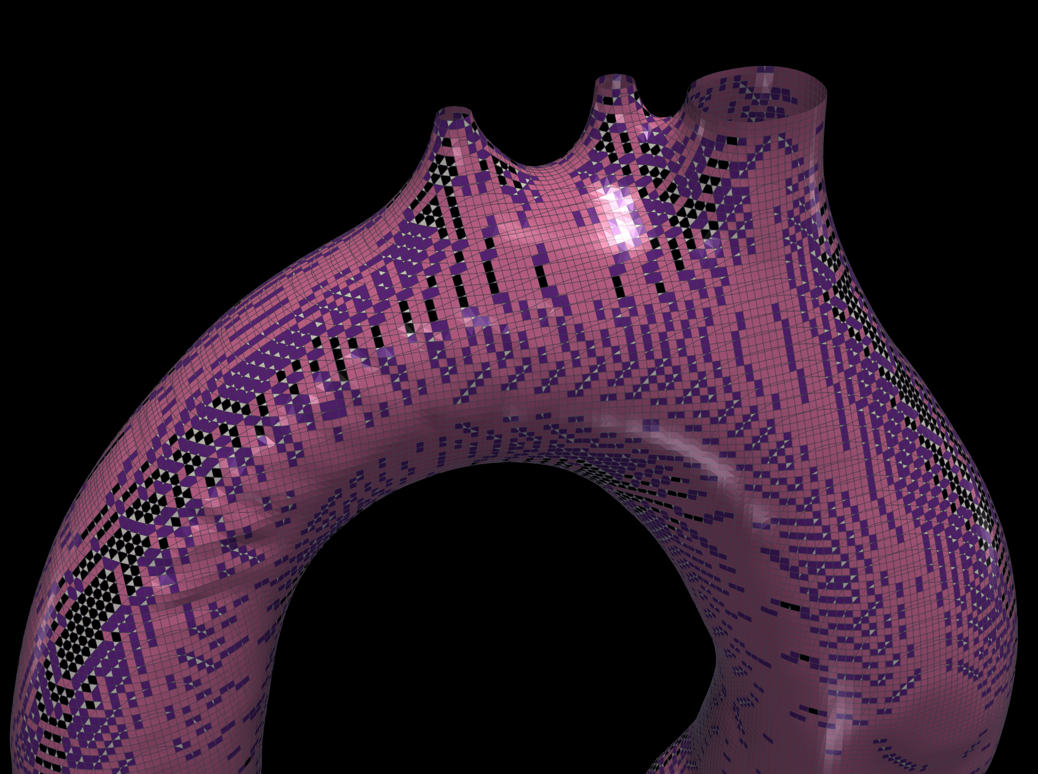
(a) Cut-cell facets forming the discretised boundary $\Gamma_{h}$.

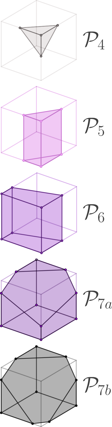
(b) Cut-cell types

Figure 5: In cut-cell FEM the boundary, $\Gamma$, is implicitly defined by the zeroth level-set of ${\varphi_{\pm}}$. The discretised boundary, $\Gamma_{h}$, consists of the facets of the cut-cells. Under the assumption of a geometry-resolving mesh, there are only a few different cut-cell types (polyhedra, $\mathcal{P}$, formed by cuboid-plane intersections).

4.1.1 Discrete weak form of the Navier–Stokes problem

The discrete weak form of the N–S problem, $\mathscr{M}_{h}$, is given by

$$\mathscr{M}_{h}\coloneqq\mathscr{M}(\bm{u}_{h},p_{h},\bm{v}_{h},q_{h};\bm{x})+\underbrace{s^{\nabla\text{div}}_{{u}_{h}}(\bm{v}_{h},\bm{u}_{h})+s^{\text{CIP}}_{{u}_{h}}(\bm{v}_{h},\bm{u}_{h})+s^{\text{CIP}}_{p_{h}}(q_{h},p_{h})}_{\text{numerical stabilisation terms}}=0\quad,$$ (77)

where $\mathscr{M}$ is given by (31), and the numerical stabilisation terms are given by

$$s^{\nabla\text{div}}_{{u}_{h}}(\bm{v}_{h},\bm{u}_{h})\coloneqq \sum_{{\mathchoice{\makebox[25.72093pt]{$\displaystyle K\in\mathcal{T}_{h}\cap\Omega$}}{\makebox[25.72093pt]{$\textstyle K\in\mathcal{T}_{h}\cap\Omega$}}{\makebox[16.0878pt]{$\scriptstyle K\in\mathcal{T}_{h}\cap\Omega$}}{\makebox[11.88501pt]{$\scriptscriptstyle K\in\mathcal{T}_{h}\cap\Omega$}}}}{{c_{\nabla\text{div},K}}}\ \big{\langle}\nabla\bm{\cdot}\bm{v}_{h},\nabla\bm{\cdot}\bm{u}_{h}\big{\rangle}_{K\cap\Omega}\quad,$$ (78a)

$$s^{\text{CIP}}_{{u}_{h}}(\bm{v}_{h},\bm{u}_{h})\coloneqq \sum_{F\in\mathcal{F}_{i}}{\mathchoice{\makebox[23.32869pt]{$\displaystyle c_{{u},F}$}}{\makebox[23.32869pt]{$\textstyle c_{{u},F}$}}{\makebox[16.60152pt]{$\scriptstyle c_{{u},F}$}}{\makebox[15.73601pt]{$\scriptscriptstyle c_{{u},F}$}}}\ \big{\langle}[\nabla\bm{v}_{h}],[\nabla\bm{u}_{h}]\big{\rangle}_{F}\quad,$$ (78b)

$$s^{\text{CIP}}_{p_{h}}(q_{h},p_{h})\coloneqq \sum_{F\in\mathcal{F}_{i}}{\mathchoice{\makebox[23.32869pt]{$\displaystyle c_{p,F}$}}{\makebox[23.32869pt]{$\textstyle c_{p,F}$}}{\makebox[16.60152pt]{$\scriptstyle c_{p,F}$}}{\makebox[15.73601pt]{$\scriptscriptstyle c_{p,F}$}}}\ \big{\langle}[\nabla q_{h}],[\nabla p_{h}]\big{\rangle}_{F}\quad.$$ (78c)

where $\mathcal{F}_{i}$ is the set of interior facets, and $[\cdot]$ is the jump of a function along the face $F$, as defined in [MSW18]. For the numerical method to be robust in a variety of flow conditions, the Nitsche penalty parameters, $\eta_{\Delta}$, $\eta_{\nabla}$, and the stabilisation coefficients, $c_{\nabla\text{div},K}$, $c_{{u},F}$, and $c_{p,F}$, must all scale with the flow. Appropriate voxel-wise constant formulas are given by [Cod02, MSW18]

$$\eta_{\Delta}=\gamma_{\mathscr{N}}~{}h^{-1}\lVert\nu_{e}\rVert_{L^{\infty}(K)}\quad,\quad\eta_{\nabla}=\gamma_{\mathscr{N}}~{}h^{-1}\phi_{u,K}\quad,$$ (79a)

$$c_{\nabla\text{div},K}\coloneqq{\gamma_{\nabla\text{div}}}~{}\big{(}\lVert\nu_{e}\rVert_{L^{\infty}(K)}+h\lVert\bm{u}_{k}\rVert_{L^{\infty}(K)}\big{)}\quad,$$ (79b)

$$c_{u,F}\coloneqq\left\{\begin{array}[]{ll}c_{u,F_{i}}&,~{}F\in\mathcal{F}_{i}\setminus\mathcal{F}_{\Gamma}\\ {\gamma_{\nu}}~{}h\lVert\nu_{e}\rVert_{L^{\infty}(K)}+{c_{{u},F_{i}}}&,~{}F\in\mathcal{F}_{\Gamma}\\ \end{array}\right.\quad,\quad c_{u,F_{i}}\coloneqq{\gamma_{{u}}}~{}h\lVert\bm{u}_{k}\rVert_{L^{\infty}(F)}^{2}~{}\langle\phi_{p}\rangle\lvert_{F}\quad,$$ (79e)

$$\phi_{p,K}\coloneqq{h^{2}\phi_{{u},K}^{-1}}\quad,\quad\phi_{{u},K}\coloneqq\lVert\nu_{e}\rVert_{L^{\infty}(K)}+{c_{{u}}}h\lVert\bm{u}_{k}\rVert_{L^{\infty}(K)}\quad,\quad{c_{p,F}}\coloneqq{\gamma_{p}}~{}h\langle\phi_{p}\rangle\lvert_{F}\quad,$$ (79f)

where $\bm{u}_{k}$ is the velocity field at iteration $k$, $\mathcal{F}_{\Gamma}\subset\mathcal{F}_{i}$ is the set of boundary facets, and $\langle\cdot\rangle\lvert_{F}$ is the face average value between two neighboring voxels [MSW18]. Typical values for the numerical parameters are

$$\begin{array}[]{c c c c c c}\gamma_{\mathscr{N}}&\gamma_{\nabla\text{div}}&\gamma_{u}&\gamma_{p}&\gamma_{\nu}&c_{u}\\ (30,100)&(0.1,1)&(0.01,0.1)&(0.01,0.1)&(0.01,0.1)&(0.1,1)\end{array}\quad.$$ (82)

The numerical (Galerkin) problem is thus to find $(\bm{u}_{h},p_{h})\in\bm{M}_{h}\times M_{h}$ such that (77) holds true for all $(\bm{v}_{h},q_{h})\in\bm{M}_{h}\times M_{h}$. The stabilised cut-cell finite element method is adopted from [MSW18]. In this study we slightly modify the formulation by including $\nabla$-div stabilisation in order to improve the condition number of the Schur complement [BO06, Ols+09, HR13].

4.1.2 Discrete weak form of the viscous Eikonal problem

The discrete weak form of the viscous Eikonal problem, $\mathscr{D}_{h}$, is given by

$$\mathscr{D}_{h}\coloneqq\mathscr{D}(r_{h},{\varphi_{\pm}}_{h})+s^{\text{CIP}}_{u_{h}}(r_{h},{\varphi_{\pm}}_{h})=0\quad,$$ (83)

where $\mathscr{D}$ is given by (61), and the CIP stabilisation term, $s^{\text{CIP}}_{u_{h}}(\cdot,\cdot)$, was defined in section 4.1.1. We further define the smoothed sign function

$$\mathrm{sgn}_{h}({\varphi_{\pm}}_{h})\coloneqq\frac{{\varphi_{\pm}}_{h}}{\sqrt{{\varphi^{2}_{\pm}}_{h}+h^{2}}}\quad,$$ (84)

which replaces the sign function, $\mathrm{sgn}(x)\coloneqq x/\lvert x\rvert$, of (61) in the case of the discrete problem. As in section 4.1.1, the numerical (Galerkin) problem is to find ${\varphi_{\pm}}_{h}\in M_{h}$ such that (83) holds true for all $r_{h}\in M_{h}$.

4.2 Cut-cell integration

For the numerical evaluation of integrals we use standard Gaussian quadrature for intact cells, $K\in\mathcal{T}_{h}^{\scaleobj{0.7}{\Box}}$. For cut-cells, $K\in\mathcal{T}_{h}^{\triangleright}$, however, integration must be considered only on the intersection $K\cap\Omega$ for volumetric integrals and on $K\cap\Gamma$ for surface integrals. We therefore generalise the approach of [Mir96], which relies on the divergence theorem and replaces the integral over $K\cap\Omega$ with an integral over $\partial\big{(}K\cap\Omega\big{)}$. The boundary integral on $\partial\big{(}K\cap\Omega\big{)}$ is then easily computed using one-dimensional Gaussian quadrature [MLL13]. For instance, let us consider that we want to compute the integral of the Laplacian in a cut-voxel, $\mathcal{P}$, given by

$$A_{pq}=\int_{\mathcal{P}}\nabla\varphi_{p}\bm{\cdot}\nabla\varphi_{q}\quad.$$ (85)

If $\varphi$ is a polynomial test function, we can find coefficients ${\color[rgb]{0,0,0}c_{pqk}}$ such that

$$A_{pq}=\sum_{k}{\color[rgb]{0,0,0}c_{pqk}}\int_{\mathcal{P}}x^{\alpha^{k}}\quad,$$ (86)

for a multi-index $\alpha^{k}$. In general, any integral of the weak (Galerkin) formulation can be expressed in the form of (86). The problem is then to i) find the coefficients $c_{pqk}$, and ii) compute the monomial integrals

$$I^{\mathcal{P}}_{k}=\int_{\mathcal{P}}x^{\alpha^{k}}\quad.$$ (87)

For polynomial test functions, the coefficients $c_{pqk}$ are easily obtained using symbolic mathematics [Meu+17]. They only depend on the integrand, which depends on the boundary value problem at hand, and can thus be stored in a computer file. The monomial integrals, $I^{\mathcal{P}}_{k}$, depend on the geometry, $\mathcal{P}$, and therefore need to be computed as a pre-processing step before assembling the FEM system matrix. For every cut-cell, the monomial integrals that are needed can be computed only once and stored in memory in order to avoid unnecessary extra calculations. The monomial integrals are evaluated only for the cut-cells, $K\in\mathcal{T}_{h}^{\triangleright}$. Hence, the numerical cost is negligible compared to other bottlenecks in the algorithm, such as the linear system solution. The algorithm to compute $I^{\mathcal{P}}_{k}$, which generalises the methodology presented originally in [Mir96], is described in [Kon23, Appendix D].

4.3 Exact pressure projection via the Schur complement

The ($\bm{u}_{h}$,$p_{h}$)-system that results after assembling the discrete weak form (31), is given by

$$\begin{pmatrix}A&B\\ -B^{*}&D\end{pmatrix}\begin{pmatrix}\bm{u}_{h}\\ p_{h}\end{pmatrix}=\begin{pmatrix}\bm{f}\\ g\end{pmatrix}\quad,$$ (88)

and has a non-zero pressure-pressure block, i.e. $D\neq 0$ (in contrast to (67)) due to the pressure stabilisation term, $s^{\text{CIP}}_{p_{h}}(q_{h},p_{h})$, which has been added in the discrete weak form. Multiplying the first equation of (88) by $A^{-1}$, and substituting it into the second equation, we obtain

$$Sp_{h}=-B^{*}A^{-1}\bm{f}-g\quad,$$ (89)

where $S\equiv\big{(}-B^{*}A^{-1}B-D\big{)}$ is the Schur complement. After solving (89) for $p_{h}$, $\bm{u}_{h}$ can be obtained by solving

$${A\bm{u}_{h}=\bm{f}-Bp_{h}}\quad.$$ (90)

Equivalently, we can write the coupled system (88) in its decoupled form

$$\begin{pmatrix}A&0\\ 0&S\end{pmatrix}\begin{pmatrix}\bm{u}_{h}\\ p_{h}\end{pmatrix}=\begin{pmatrix}\bm{f}-BS^{-1}\big{(}-B^{*}A^{-1}\bm{f}-g\big{)}\\ -B^{*}A^{-1}\bm{f}-g\end{pmatrix}\quad.$$ (91)

It is worth noting that $S$ is not necessarily sparse, and thus it cannot be assembled. Instead, $S$ is treated as a matrix-vector product operator. This implies that, when an iterative algorithm is used for (89), a linear system with the velocity-velocity subblock, $A$, is solved at every pressure iteration. For the exact projection method to be efficient we therefore require good preconditioners for both $S$ and $A$. We also use $\nabla$-div stabilisation for Schur-complement preconditioning, which amounts to adding $s^{\nabla\text{div}}_{{u}_{h}}(\bm{v}_{h},\bm{u}_{h})$ to the discrete weak form [HR13]. We then use the approximation of $S$,

$$\widetilde{S}\coloneqq-B^{*}\big{(}\textrm{diag}(A)\big{)}^{-1}B-D\quad,$$ (92)

as the preconditioner of the iterative pressure solver.

4.4 Implementation

The Bayesian inverse Navier–Stokes solver, which incorporates the cut-cell FEM solver, is implemented in Python using MPI (mpi4py, [DPS05]) and PETSc (petsc4py) [Bal+22, Bal+22a]. We solve (89) using FGMRES [Saa93] for the outer iterations (pressure iterations), and GMRES [SS86] for the inner iterations (velocity subblock, $A$, iterations). We precondition the inner solver using either the overlapping additive Schwarz method (ASM) [WD87], with ILU(0) for each subdomain, or generalised algebraic multigrid (GAMG). In our implementation, ASM is more efficient when run on a workstation, and for relatively small problems, while GAMG performs and scales better in high performance computing clusters. When solving with $\widetilde{S}$, we use GMRES with GAMG. A similar setup is used to solve the viscous Eikonal problem. The uncertainties around the MAP solution can be estimated by computing the eigendecomposition of either the exact or the approximated posterior covariance operators, as was described in section 2.3.1. This requires the integration of a large-scale eigenvalue problem solver, such as SLEPc [HRV05] (slepc4py), into the current software, which is the subject of future work.

5 Reconstruction of flow-MRI data in an aortic arch

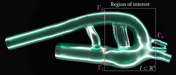
(a) Physical model and b.c. setup

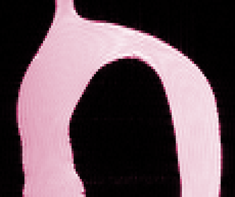
(b) spin density (2D slice of ROI)

Figure 6: 3D-printed (rigid) physical model of an aortic arch and boundary condition setup (figure 6(a)). We have obtained flow-MRI data of the full geometry, but we only reconstruct the flow in the region of interest (ROI), $I$, which is enclosed in a cuboid in $\mathbb{R}^{3}$. To reconstruct the flow in $I$, we only use the flow-MRI data inside $I$. That is, $I_{d}\equiv I_{m}\equiv I$.

In this section we demonstrate algorithm 1 by reconstructing flow-MRI data of a steady laminar flow through a physical model of an aortic arch at two different flow conditions: i) low $\mathit{Re}$ and ii) high $\mathit{Re}$, and for two different signal-to-noise ratios (SNR): i) low SNR ($\sim 5$) and ii) high SNR ($>200$).

5.1 Problem setup

The model geometry, which is shown in figure 6(a), is taken from a computed tomography scan and was 3D-printed using stereolithography (resin-printing). The characteristic length, based on the inlet diameter, is $L=1.3$ cm, and the characteristic velocity is defined as $U\equiv Q/A$, where $Q$ is the volumetric flow rate, and $A$ is the cross-sectional area of the inlet, $\Gamma_{i}$. In the low $\mathit{Re}$ case we have $\mathit{Re}=554$ ($=UL/\nu$), where $U=4.26$ cm/s, and in the high $\mathit{Re}$ case we have $\mathit{Re}=1526$ ($=UL/\nu$), where $U=11.74$ cm/s. The field of view (FOV) is $5.39\times 2.53\times 4.51$ cm, which is the region of interest (ROI) (shown in figure 6(a)), and is the same for both the data space and the model space. That is, we reconstruct the flow in the ROI using only the flow-MRI data inside the ROI. The number of voxels and the resolution in the data space and the model space are shown in table 1. Note that, the total number of active voxels in the model space are $\sim 670\times 10^{3}$, consisting of $\sim 590\times 10^{3}$ interior intact voxels and $\sim 80\times 10^{3}$ cut voxels. For this geometry we have obtained quantitatively accurate high SNR ($>200$) flow-MRI (phase-contrast MRI) data, which we corrupt with Gaussian white noise in order to generate the low SNR ($\sim 5$) flow-MRI data. (Further details regarding the flow-MRI experiment can be found in [Kon23, Appendix E.2], and the SNR is computed as in [KJ23, Section III.A].) The noise magnitude of the low SNR and the high SNR data is shown in table 1. In the N–S problem (28), we set a no-slip (zero-Dirichlet) b.c. on the aorta walls, $\Gamma$, a Dirichlet (velocity) boundary condition, $\bm{g}_{i}$, on the ascending aorta inlet, $\Gamma_{i}$, and natural boundary conditions, $\bm{g}_{o}$, on the aorta outlets, $\Gamma_{o}$, which are four in total, consisting of the three upper branches and the descending aorta (shown in figure 6(a)).

data and model domain
data voxels	data resolution	model voxels	model resolution
$115\times 54\times 77$	$469\times 469\times 586$ $\mu$m	$207\times 97\times 174$	$260\times 260\times 260$ $\mu$m

data noise level $(\sigma_{u^{\star}_{x}},\sigma_{u^{\star}_{y}},\sigma_{u^{\star}_{z}})/U$
	low SNR	high SNR	$U$ (cm/s)
low $\mathit{Re}$	$(0.519,0.519,0.519)$	$(0.011,0.010,0.011)$	$4.26$
high $\mathit{Re}$	$(0.544,0.544,0.545)$	$(0.012,0.012,0.020)$	$11.74$

prior covariance ($\mathcal{C}_{\bar{\bm{x}}}$) and vSDF parameters
$\sigma_{\varphi_{\pm}}$	$\sigma_{\bm{g}_{i}}/U$	$\sigma_{\bm{g}_{o}}L/U$	$\sigma_{\nu}$	$\ell_{\bm{g}_{i}}$	$\ell_{\bm{g}_{o}}$	$\mathit{Re}_{\varphi_{\pm}}$	$\ell_{\Gamma}$
$h^{\text{max}}_{\text{MRI}}\simeq 2.25h$	$(\sigma_{u^{\star}_{x}},\sigma_{u^{\star}_{y}},\sigma_{u^{\star}_{z}})$	$(10,10,10)$	$10^{-4}$	$h$	$h$	$4$	$h$

numerical parameters (cut-cell FEM)
$\gamma_{\mathcal{N}}$	$\gamma_{\nu}$	$\gamma_{u}$	$\gamma_{p}$	$\gamma_{\nabla\text{div}}$	$c_{u}$
$100$	$0.05$	$0.05$	$0.05$	$1$	$1/6$

Table 1: Problem setup and input parameters for the Bayesian inverse N–S problem.

5.2 Prior means for the N–S unknowns

We obtain a level-set function, $\psi$, of the prior mean geometry, $\bar{\Omega}$, using Chan–Vese segmentation [CV01, Get12] on the magnitude images (spin density) of the flow-MRI data (see figure 6(b)). We then solve the vSDF problem (71) to obtain the prior mean of the vSDF, $\bar{\varphi}_{\pm}$. The prior mean of the inlet b.c., $\bar{\bm{g}}_{i}$, is obtained by solving

$$\big{(}\mathrm{I}-\ell_{0}^{2}\widetilde{\Delta}\big{)}\,\bar{\bm{g}}_{i}=\big{(}\mathcal{S}^{*}\bm{u}^{\star}\big{)}\big{|}_{\Gamma_{i}}\quad\text{on}\quad\Gamma_{i}\quad,$$ (93)

where $\ell_{0}=3h$, $\widetilde{\Delta}$ is the ${L}^{2}$-extension of the Laplacian that incorporates the zero-Dirichlet (no-slip) b.c. on $\partial\Gamma_{i}$, and $\big{(}\mathcal{S}^{*}\bm{u}^{\star}\big{)}\big{|}_{\Gamma_{i}}$ is the restriction of the model-space projection of the flow-MRI data on the inlet, $\Gamma_{i}$. The prior mean of the outlet (natural) b.c., $\bar{\bm{g}}_{0}$, is set to $\bar{\bm{g}}_{0}\equiv(0,0,0)$ due to lack of information, hence the high uncertainty (see table 1). Because we used a Newtonian fluid (water) in the flow-MRI experiments, the effective viscosity, $\nu_{e}$, is assumed to be constant in $\Omega$, and is set to $\bar{\nu}_{e}=UL/\mathit{Re}$. The prior covariance operator, $\mathcal{C}_{\bar{\bm{x}}}$, is constructed using the values of table 1, as explained in section 3.3. It is important to note that the prior means for ${\varphi_{\pm}}$ and $\bm{g}_{i}$ are generated from the flow-MRI data that we reconstruct. That is, we do not perform any additional experiment in order to obtain higher-quality priors (e.g. a computed tomography scan for the geometry or a high-resolution flow-MRI scan for the geometry and the inlet b.c.). The prior means for $\bm{g}_{o}$ and $\nu_{e}$, however, cannot be extracted from the flow-MRI scans, and, therefore, depend on the prior knowledge of the problem.

5.3 Reconstruction results

We demonstrate algorithm 1 at two different flow conditions and two different SNRs for the 3D steady laminar flow in the ROI of the aortic arch (see table 2 for notation). We apply the algorithm on low SNR flow-MRI data, $\bm{u}^{\star}$, in order to infer the maximum a posteriori (MAP) estimate, $\bm{u}^{\circ}$, which is the most probable reconstructed velocity field. This highlights the capability of algorithm 1 to accurately reconstruct flow features that are obscured by noise, which relies on the explanatory power of the generalised Navier–Stokes problem. We also apply the algorithm on high SNR flow-MRI data, $\bm{u}^{\bullet}$, (i.e. $\bm{u}^{\star}\mathrel{\reflectbox{$\mapsto$}}\bm{u}^{\bullet}$ in algorithm 1) in order to infer the MAP estimate, $\bm{u}^{\mathbin{\text{\ooalign{\raisebox{0.0pt}{\leavevmode\leavevmode\hbox{ \leavevmode\hbox to3.5pt{\vbox to3.11pt{\text{[drawing]}}}}}\cr$\circ$\cr}}}}$. This highlights the capability of algorithm 1 to reproduce (fit) the high-quality velocity images, and helps us identify model-data discrepancies other than Gaussian white noise (i.e. modelling and/or experimental biases).

data	prior	reconstruction
$\bm{u}^{\star}/\bm{u}^{\bullet}$	$\bar{\bm{u}}/\widetilde{\bm{u}}$	$\bm{u}^{\circ}$/$\bm{u}^{\mathbin{\text{\ooalign{\raisebox{0.0pt}{\leavevmode\leavevmode\hbox{ \leavevmode\hbox to3.15pt{\vbox to2.8pt{\text{[drawing]}}}}}\cr$\circ$\cr}}}}$

Table 2: Notation for the low$/$high SNR reconstruction cases.

5.3.1 Velocity field reconstruction at low $\mathit{Re}$

The reconstruction results for the low $\mathit{Re}$ ($=554$) case are shown in figure 7. We observe that the low SNR reconstruction, $\bm{u}^{\circ}$, obtained from the low SNR data, $\bm{u}^{\star}$, is almost indistinguishable from the high SNR data, $\bm{u}^{\bullet}$, and the high SNR reconstruction, $\bm{u}^{\mathbin{\text{\ooalign{\raisebox{0.0pt}{\leavevmode\leavevmode\hbox{ \leavevmode\hbox to3.5pt{\vbox to3.11pt{\text{[drawing]}}}}}\cr$\circ$\cr}}}}$, except for minor discrepancies. Also, the high SNR reconstruction, $\bm{u}^{\mathbin{\text{\ooalign{\raisebox{0.0pt}{\leavevmode\leavevmode\hbox{ \leavevmode\hbox to3.5pt{\vbox to3.11pt{\text{[drawing]}}}}}\cr$\circ$\cr}}}}$, obtained from the high SNR data, $\bm{u}^{\bullet}$, fits the data with visually imperceptible error. We reach the same conclusions by inspecting the data-model discrepancies of figure 8. In the low SNR case, algorithm 1 manages to assimilate physically relevant information, which appears in the form of coherent structures immersed in Gaussian white noise, while filtering out noise and artefacts. The same applies to the high SNR case, the only difference being that model and/or flow-MRI experimental biases dominate the data-MAP residuals over white noise. For this reason, the characteristic scale for the discrepancy is chosen to be $U$, instead of the noise variance, $\sigma^{2}$. For this $\mathit{Re}$ number, it is sensible to assume that the bias comes mainly from the flow-MRI experiment because the flow is steady and laminar, and the Newtonian viscosity model describes water to high accuracy. Consequently, the N–S problem (28) can model the velocity field to high accuracy.

5.3.2 Velocity field reconstruction at high $\mathit{Re}$

The reconstruction results for the high $\mathit{Re}$ ($=1526$) case, shown in figures 9 and 10, can be interpreted in the same way. In the high $\mathit{Re}$ case, however, the velocity field has a richer, finer structure, and sharper gradients compared with the low $\mathit{Re}$ case. This showcases the capability of algorithm 1 to reconstruct details of the flow that are completely obscured by noise. In the low SNR case, we observe that the data-MAP residuals (figure 10) approximate white noise almost everywhere except for two regions: i) the upper main branch, and ii) the descending aorta. Both regions involve recirculation zones and local flow separation (see $\bm{u}^{\bullet}$ and $\bm{u}^{\mathbin{\text{\ooalign{\raisebox{0.0pt}{\leavevmode\leavevmode\hbox{ \leavevmode\hbox to3.5pt{\vbox to3.11pt{\text{[drawing]}}}}}\cr$\circ$\cr}}}}$ in figure 9). In the high SNR case, we observe that the data-MAP residuals are, in contrast to the low $\mathit{Re}$ case, non-negligible, and that their peak magnitude is at the recirculation region of the descending aorta. For this near-critical $\mathit{Re}$ number, it is possible that the laminar flow transitions to (weakly) turbulent flow in the vicinity of the recirculation bubbles, particularly at the descending aorta [Man+24, Figure 5]. Since flow-MRI data are, to a certain extent, averaged (e.g. due to cross-voxel motion and asynchronous spatial and velocity encoding in the MRI sequence), and given that the high SNR flow-MRI scan acquisition time was $\sim 3.5$ hours per velocity component [Kon23, Appendix E.2], it is possible that flow fluctuations during the course of the experiment (e.g. due to temperature and flow rate changes or bubbles) have slightly distorted the velocity images. It is also expected for this averaging bias to increase in magnitude as the $\mathit{Re}$ number increases, since the flow becomes more susceptible to external perturbations.

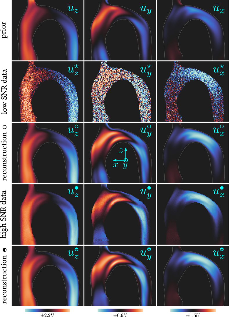
Figure 7: We apply algorithm 1 on low/high SNR data $\bm{u}^{\star}$/$\bm{u}^{\bullet}$ for the low $\mathit{Re}$ flow ($U=4.26$ cm/s). The algorithm first generates a prior velocity field, $\bar{\bm{u}}/\widetilde{\bm{u}}$, and then solves a Bayesian inverse N–S problem in order to find the most likely (MAP) reconstruction, $\bm{u}^{\circ}$/$\bm{u}^{\mathbin{\text{\ooalign{\raisebox{0.0pt}{\leavevmode\leavevmode\hbox{ \leavevmode\hbox to3.15pt{\vbox to2.8pt{\text{[drawing]}}}}}\cr$\circ$\cr}}}}$. The prior $\widetilde{\bm{u}}$, which is generated from the high SNR data, $\bm{u}^{\bullet}$, is similar to $\bar{\bm{u}}$ and thus not shown.

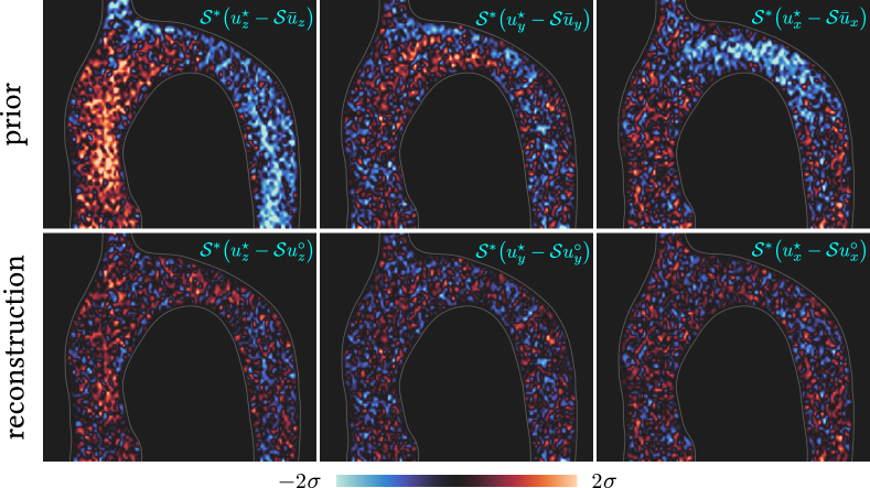
(a) velocity residuals at low SNR

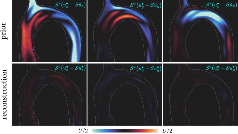
(b) velocity residuals at high SNR

Figure 8: Data-model discrepancies (reconstruction residuals) projected onto the model space, $\bm{M}$, for the low SNR case (figure 8(a)) and the high SNR case (figure 8(b)) of the low $\mathit{Re}$ flow. In the low SNR case, coherent structures in the initial residual (data-prior discrepancy) are assimilated and the final residual (data-MAP discrepancy) approximates Gaussian white noise with variance $\sigma^{2}$. In the high SNR case the results are similar with the exception that experimental (flow-MRI) biases dominate over noise and the characteristic scale of the error is based on $U$.

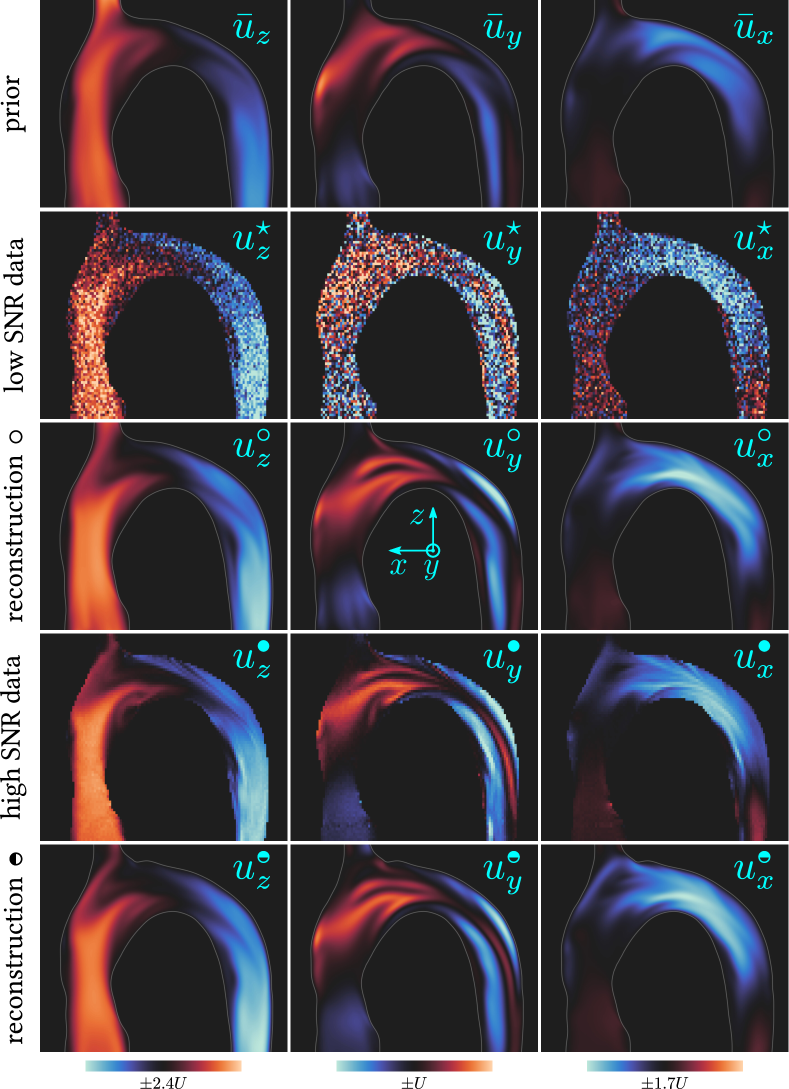
Figure 9: As for figure 7 but for the high $\mathit{Re}$ flow ($U=11.74$ cm/s).

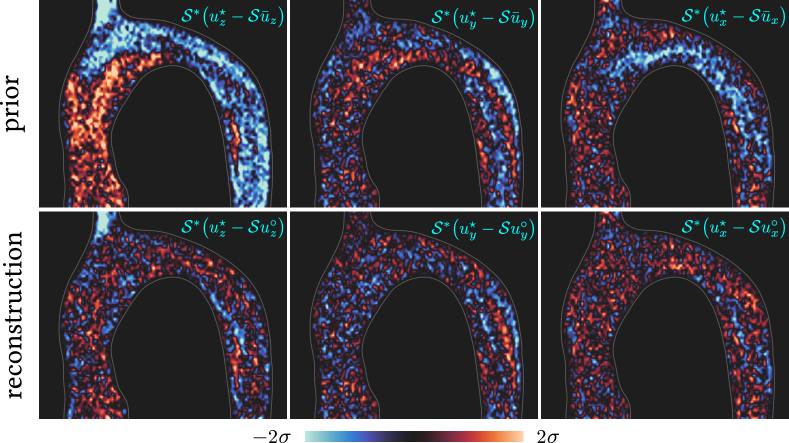
(a) velocity residuals at low SNR

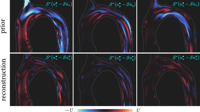
(b) velocity residuals at high SNR

Figure 10: As for figure 8 but for the high $\mathit{Re}$ flow.

5.3.3 Mean reconstruction errors

We quantitatively compare the reconstructions by defining the mean reconstruction error

$$\bm{\mathcal{E}}\coloneqq\lvert{\Omega}\rvert^{-1}\big{\|}\bm{u}_{\text{data}}-\mathcal{S}\bm{u}_{\text{model}}\big{\|}_{L^{2}(I_{d})}\quad,$$ (94)

where $\bm{u}_{\text{data}}\in(\bm{u}^{\star},\bm{u}^{\bullet})$, $\bm{u}_{\text{model}}\in(\bar{\bm{u}},\widetilde{\bm{u}},\bm{u}^{\circ},\bm{u}^{\mathbin{\text{\ooalign{\raisebox{0.0pt}{\leavevmode\leavevmode\hbox{ \leavevmode\hbox to3.5pt{\vbox to3.11pt{\text{[drawing]}}}}}\cr$\circ$\cr}}}})$, and $\lvert\Omega\rvert$ is the volume of $\Omega$.

For the low SNR case, we examine the $\sigma_{u^{\star}}$-normalised errors, $(\mathcal{E}/{\sigma}_{u^{\star}})_{i}$, because the noise dominates the residuals (see figures 8(a), 10(a)). Under the assumption of Gaussian white noise, an ideal reconstruction of the low SNR data (i.e. one that perfectly assimilates the data without fitting noise) is expected to have a mean reconstruction error $(\mathcal{E}/{\sigma}_{u^{\star}})_{i}=1$. In practice, however, imperfections in the data, such as artefacts, outliers, and interference noise, increase the kurtosis of the distribution (fat-tailed distribution). Thus, values higher than $1$ may correspond to an ideal reconstruction. In general, under the assumption of Gaussian white noise, $(\mathcal{E}/{\sigma}_{u^{\star}})_{i}\gg 1$ implies that the reconstruction algorithm did not succeed in assimilating all the information (e.g. due to experimental or model biases), while $(\mathcal{E}/{\sigma}_{u^{\star}})_{i}\ll 1$ implies that the reconstruction overfits the data. In the extreme case of $(\mathcal{E}/{\sigma}_{u^{\star}})_{i}=0$, we have that $\bm{u}_{\text{data}}\equiv\mathcal{S}\bm{u}_{\text{model}}$, i.e. there is no reconstruction. For the low $\mathit{Re}$ case, we find that the MAP reconstruction is ideal, in the sense that the MAP mean errors are near $1.00$ (see table 3). For the high $\mathit{Re}$ case, the mean errors are larger than $1.00$, which is due to the model/experimental biases that we have attributed to the $\mathit{Re}$ number being near-critical (see section 5.3.2). However, the MAP mean errors are significantly lower than the prior mean errors, showing that the algorithm has managed to assimilate useful information.

For the high SNR case, we examine the errors $(\mathcal{E}/U)_{i}$ because the experimental/model bias dominates the residuals (see figures 8(b), 10(b)). We find that for both the low and high $\mathit{Re}$ cases there is a significant reduction in the mean error (see table 3). For the low $\mathit{Re}$ case, the MAP reconstruction fits the high SNR data with high accuracy and the mean errors are negligible. For the high $\mathit{Re}$ case, the mean errors are non-negligible due to the model/experimental biases that we have attributed to the near-critical $\mathit{Re}$ number (see section 5.3.2). For comparison, volumetric flow rates calculated from the flow-MRI images, in the ascending portion of the aorta, agreed with volumetric flow rates measured from the pump outlet within an average error of $\pm 0.04U$.

prior velocity field
	low SNR ($\bm{\mathcal{E}}/\bm{\sigma}_{u^{\star}}$)	high SNR ($\bm{\mathcal{E}}/U$)
low $\mathit{Re}$	$(1.09,1.04,1.23)$	$(0.21,0.14,0.30)$
high $\mathit{Re}$	$(1.20,1.21,1.54)$	$(0.32,0.34,0.52)$
posterior (MAP) velocity field
	low SNR ($\bm{\mathcal{E}}/\bm{\sigma}_{u^{\star}}$)	high SNR ($\bm{\mathcal{E}}/U$)
low $\mathit{Re}$	$(1.00,1.00,1.02)$	$(0.04,0.04,0.06)$
high $\mathit{Re}$	$(1.07,1.06,1.12)$	$(0.17,0.15,0.24)$

Table 3: Mean reconstruction errors for the prior and the posterior (MAP) velocity fields.

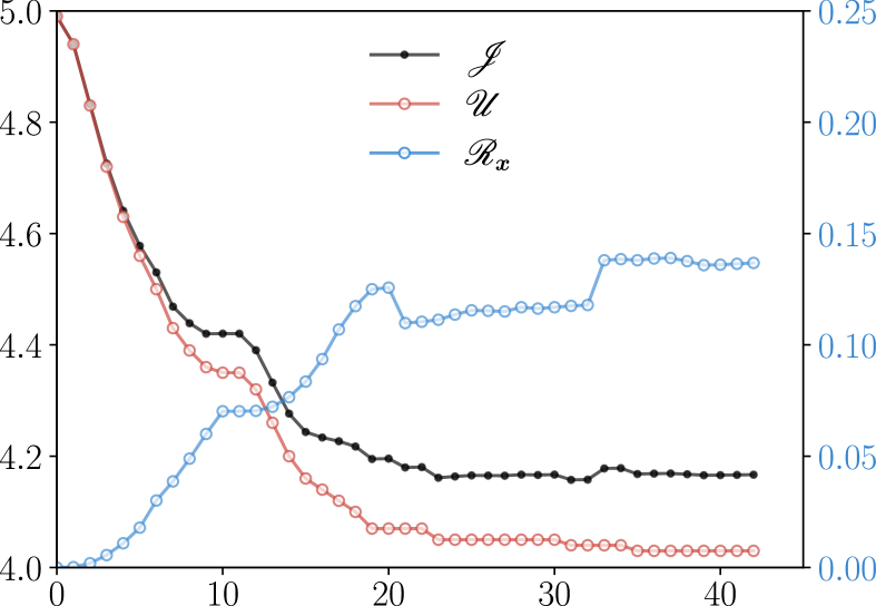
(a) low $\mathit{Re}$, low SNR

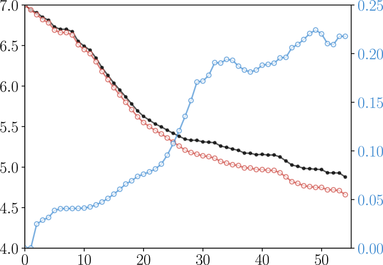
(b) high $\mathit{Re}$, low SNR

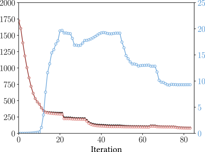
(c) low $\mathit{Re}$, high SNR

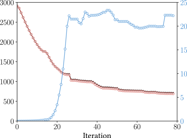
(d) high $\mathit{Re}$, high SNR

Figure 11: Optimisation log depicting the evolution of the objective functional, $\mathscr{J}$, the model-data discrepancy, $\mathscr{U}$, and the priors, $\mathscr{R}_{\bm{x}}$, for the four different inverse problems.

Figure 11 shows the optimisation logs of the four reconstruction problems. Note that the high SNR reconstruction problems converge more slowly than the low SNR reconstruction problems because there is more information to be assimilated.

5.4 Explanatory power and interpretability of the N–S problem

It is worth noting that the N–S unknowns, $\bm{x}$, as chosen in this study, correspond to physical quantities that are interpretable. For example, in cardiovascular applications, the fluid domain, $\Omega$, defines the geometry of the blood vessel, the boundary condition $\bm{g}_{i}$ defines the inlet velocity, the boundary condition $\bm{g}_{o}$ defines the fluid stresses at the outlets, and the effective kinematic viscosity, $\nu_{e}$, depends on the rheological properties of the fluid [KHM24]. Although we have neglected the equations of elastodynamics, we have not fixed the shape of $\Omega$. Therefore, for unsteady flows and compliant walls, we can still infer the movement of the geometry and its influence on the velocity field, but we cannot yet infer the elastic properties of the walls.

Another important aspect regarding the choice of the N–S parameters, $\bm{x}$, is that they have limited control over the modelled velocity field, $\bm{u}$. More precisely, every N–S unknown is a function defined on a $(d-1)$-manifold, where $d$ is the dimension of the problem. This means that the inverse N–S problem is a sparsifying transform [KJ23] that maps velocity fields, defined on a subset of $\mathbb{R}^{d}$, to N–S unknowns, defined on a subset of $\mathbb{R}^{d-1}$ (see table 4). In contrast, the inverse, forced N–S problem, which is obtained after adding a volumetric forcing term, $\bm{f}$, to the momentum equation in order to enhance control (i.e. increase model flexibility to fit the data), is no longer a sparse transformation. It can be made sparse, however, if $\bm{f}$ is parameterised such that $\bm{f}=\bm{f}(\bm{z})$, where $\bm{z}$ is an unknown defined on a $(d-1)$-manifold or a subset thereof. In addition, the inverse problem is more interpretable if $z$ has a physical meaning, which is preferable.

Because we limit the control to physically-interpretable parameters in $\mathbb{R}^{d-1}$, we rely on the explanatory power of the N–S problem, which relies on first principles, such as momentum and mass conservation, and explains much from little. This an advantage because it provides insight into the physical problem. If the model cannot explain the data then it has to be revised, which leads to an improved physical model and the advancement of fluid dynamics modelling. The process of model selection can be made even more rigorous using Bayesian inference [Mac03, Chapter 28][JY22, YJ24].

unknowns (search space)				model states		voxels
$\Gamma$	$\bm{g}_{i}$	$\bm{g}_{o}$	$\nu_{e}$	$(\bm{u},p)$	${\varphi_{\pm}}$	$\lvert\mathcal{T}_{h}\rvert$
$\mathcal{O}(n^{2})$	$\mathcal{O}(n^{2})$	$\mathcal{O}(n^{2})$	$\mathcal{O}(1)$	$\mathcal{O}(n^{3})$	$\mathcal{O}(n^{3})$	$\mathcal{O}(n^{3})$

Table 4: Dimensionality of the problem assuming a discrete domain of $\mathcal{O}(n^{3})$ voxels.

6 Summary and conclusions

We have formulated a Bayesian inverse N–S problem that assimilates noisy and sparse velocimetry data in order to jointly reconstruct the flow field and infer the unknown N–S parameters. By hardwiring a generalised N–S problem and regularising its unknown parameters using Gaussian prior distributions, the method learns the most likely (MAP) parameters in a collapsed search space. The most likely (MAP) velocity field reconstruction is then the N–S solution that corresponds to the MAP parameters. Working in a variational setting, we use a stabilised Nitsche weak form of the N–S problem that permits control of all N–S parameters, and, in particular, the Dirichlet (inlet velocity) boundary condition. We implicitly define the geometry using a viscous signed distance field, and control its regularity by choosing an appropriate artificial diffusion coefficient based on (prior) boundary smoothness assumptions. The vSDF is also implicitly defined as the solution of a viscous Eikonal boundary value problem, which is incorporated as a second constraint (the first being the N–S problem) in the saddle point problem. To solve the Bayesian inverse N–S problem we devise an iterative algorithm that searches for saddle points of the objective functional by attempting to satisfy the first order optimality conditions (i.e. solves the Euler–Lagrange system). We approximate the inverse Hessian operator of the N–S parameters, which is equivalent to the posterior covariance parameter operator, using a quasi-Newton method (BFGS). This allows us to: i) accelerate the iterative procedure using curvature information (gradient preconditioning), and ii) estimate parameter uncertainties around the MAP point (Laplace approximation). We numerically implement the algorithm using a fictitious domain cut-cell finite element method, and stabilise the numerical problem by adding symmetric and consistent stabilisation terms ($\nabla$-div and CIP) to the continuous weak form. Consequently, the numerical solution converges to the continuous solution as the background mesh size tends to zero, and the discrete formulation can be shown to be adjoint-consistent (i.e. the discretised continuous adjoint operator, $(\mathcal{G}^{*})_{h}$, is equivalent to the discrete adjoint operator, $(\mathcal{G}_{h})^{*}$).

We then apply the method to the reconstruction of flow-MRI data of a steady laminar flow through a 3D-printed physical model of an aortic arch for two different Reynolds numbers and SNR levels (low/high). We find that the method can accurately i) reconstruct the low SNR data by filtering out the noise/artefacts and recover flow features that are completely obscured by noise, and ii) reproduce (fit) the high SNR data using limited control and without overfitting (e.g. there is no volumetric forcing term in the N–S problem). In the low $\mathit{Re}$ case, the reconstructed (MAP) low SNR data are indistinguishable from the high SNR data, and the mean error of the reconstructed (MAP) high SNR data is approximately equal to the mean error of the flow-MRI experiment (as seen through the volumetric flow rate comparison between flow-MRI data and pump outlet). In the high $\mathit{Re}$ case the results are similar, but the mean reconstruction errors, although small, are non-negligible due to model/experimental biases (i.e. flow-MRI averaging and, possibly, locally turbulent flow) that we have attributed to the $\mathit{Re}$ number being near-critical.

The method described herein can increase the accuracy and the spatiotemporal resolution of velocity imaging (e.g. flow-MRI, PIV, and Doppler velocimetry) and/or significantly decrease scanning times, thus enabling the imaging of flows whose short length and/or time scales cannot be captured using state-of-the-art imaging techniques (e.g. smaller vessels such as those found in neonatal and fetal cardiology). By jointly reconstructing the flow field and learning the unknown N–S parameters, as well as their uncertainties, the method provides quantitative estimates of other derived flow quantities that are difficult to measure (e.g. pressure, wall shear stress and rheological parameters). The method requires no training, can explain much from little, is extrapolatable and is interpretable, because it hardwires prior fluid dynamics knowledge in the form of a generalised N–S problem. Consequently, it learns the most likely digital twin of the experiment, which has interesting applications in engineering design and patient-specific cardiovascular modelling. Lastly, by appropriately choosing the N–S unknowns, the inverse N–S problem is shown to be a sparsifying transform of the 3D (or 4D) velocity field. Since only the most likely (MAP) N–S unknowns need be stored to generate the flow field reconstruction, this allows the simultaneous reconstruction and compression of velocimetry data.

6.1 Future work: extensions and other applications

In this paper, we have limited our study to 3D steady laminar flows. The framework that we develop, however, readily extends to time-dependent laminar and turbulent flows, be they periodic or unsteady flows, and compliant walls. In particular, the formulation can be extended to reconstruct Reynolds-averaged turbulent flows and non-Newtonian fluid flows. This has already been done for power law fluids [KHM24], and it further extends to viscoelastic fluids. Concerning the numerics, i.e. the discrete formulation, the algorithm can greatly benefit from adaptive discretisation and multiresolution methods (in this study we used a uniform Cartesian mesh, which is suboptimal and computationally expensive). Even though the algorithm in this paper reconstructs velocimetry data, it can be extended to reconstruct raw, sparse, and noisy flow-MRI data in frequency space, as in [KJ23]. Lastly, the Bayesian inversion framework that we adopt is already set up for model comparison (e.g. ranking different viscoelastic or turbulence models based on their evidence), experimental/model bias learning (i.e. inferring the unknown unknowns) [YJ24, Section 4.2.3], and optimal experiment design [YJ24a] (e.g. design of optimal $\bm{k}$-space sampling patterns in order to accelerate flow-MRI scanning for specific types of flows).

Author contributions

AK. conceptualization, formal analysis, funding acquisition, investigation, methodology, project administration, software, validation, visualization, writing – original draft, writing – review & editing. SVE. data curation, investigation, writing – review & editing. AJS. funding acquisition, project administration, resources, supervision, writing – review & editing. MPJ. conceptualization, funding acquisition, project administration, resources, supervision, writing – review & editing.

Author ORCIDs

Alexandros Kontogiannis https://orcid.org/0000-0001-6353-3427;
Scott V. Elgersma https://orcid.org/0009-0002-4179-9747;
Andrew J. Sederman https://orcid.org/0000-0002-7866-5550;
Matthew P. Juniper https://orcid.org/0000-0002-8742-9541.

Acknowledgement

AK is supported by EPSRC National Fellowships in Fluid Dynamics (NFFDy), grant EP/X028232/1.

Appendix A Trace operators

In order to smoothly extend the boundary conditions $\bm{g}_{i}$, $\bm{g}_{o}$ to the whole domain, $I_{m}$, we introduce a modified adjoint of the trace operator. We define this adjoint trace operator, $T^{*}_{A}$, such that $\bm{v}\equiv T^{*}_{A}~{}\bm{g}$ is equivalent to solving the boundary value problem

$$\big{(}\bm{{\mathring{\bm{\nu}}}\bm{\cdot}}\nabla-\varepsilon\Delta\big{)}\bm{v}=\bm{0}\quad\text{in}~{}\Omega\quad,\quad\bm{v}=\bm{g}\quad\text{on}~{}A\quad,$$ (95)

where ${\mathring{\bm{\nu}}}$ is outward-facing unit normal vector extension, which is given by (55), and $\mathbb{R}^{+}\ni\varepsilon\ll 1$ (in this study we take $\varepsilon=h$, where $h$ is the mesh size).

Appendix B Leibniz–Reynolds transport theorem

To find the shape derivative of an integral defined in $\Omega$, when the boundary $\partial\Omega$ deforms with speed ${\mathscr{V}}$, we use the Leibniz–Reynolds transport theorem. For the bulk integral of $f:\Omega\to\mathbb{R}$, we find

$$\frac{d}{d\tau}\bigg{(}\int_{\Omega(\tau)}f\bigg{)}\bigg{|}_{\tau=0}=\int_{\Omega}f^{\prime}+\int_{\partial\Omega}f~{}({\mathscr{V}}\bm{\cdot}\bm{\nu})\quad,$$ (96)

while for the boundary integral of $f$ we find [Wal15, Chapter 5.6]

$$\frac{d}{d\tau}\bigg{(}\int_{\partial\Omega(\tau)}f\bigg{)}\bigg{|}_{\tau=0}=\int_{\partial\Omega}f^{\prime}+(\partial_{\bm{\nu}}+\kappa)f~{}({\mathscr{V}}\bm{\cdot}\bm{\nu})\quad,$$ (97)

where $f^{\prime}$ is the shape derivative of $f$ (due to ${\mathscr{V}}$), $\kappa$ is the summed curvature of $\partial\Omega$, and ${\mathscr{V}}\equiv\zeta\bm{\nu}$, with $\zeta\in L^{2}(\partial\Omega)$, is the Hadamard parameterisation of the speed field. Any boundary that is a subset of $\partial I_{m}$, i.e. the boundary of the model space $I_{m}$, is non-deforming and therefore the second term of the above integrals vanishes. The only boundary that deforms is $\Gamma$ ($\Gamma\subset\partial\Omega\subset I_{m}$).

References

• [Nit71] J. Nitsche “Über ein Variationsprinzip zur Lösung von Dirichlet-Problemen bei Verwendung von Teilräumen, die keinen Randbedingungen unterworfen sind” In Abhandlungen aus dem Mathematischen Seminar der Universität Hamburg 36.1, 1971, pp. 9–15 DOI: 10.1007/BF02995904
• [SS86] Youcef Saad and Martin H. Schultz “GMRES: A Generalized Minimal Residual Algorithm for Solving Nonsymmetric Linear Systems” In SIAM Journal on Scientific and Statistical Computing 7.3, 1986, pp. 856–869 DOI: 10.1137/0907058
• [WD87] Olof Widlund and M Dryja “An additive variant of the Schwarz alternating method for the case of many subregions”, Technical Report 339, Ultracomputer Note 131 Department of Computer Science, Courant Institute, 1987
• [SZ92] Jan Sokolowski and Jean-Paul Zolesio “Introduction to Shape Optimization” Springer Series in Computational Mathematics, Springer-Verlag, Berlin, Germany, 1992
• [Saa93] Youcef Saad “A Flexible Inner-Outer Preconditioned GMRES Algorithm” In SIAM Journal on Scientific Computing 14.2, 1993, pp. 461–469 DOI: 10.1137/0914028
• [GP95] HáKon Gudbjartsson and Samuel Patz “The Rician Distribution of Noisy MRI Data” In Magnetic Resonance in Medicine 34.6, 1995, pp. 910–914 DOI: 10.1002/mrm.1910340618
• [Mir96] Brian Mirtich “Fast and Accurate Computation of Polyhedral Mass Properties” In Journal of Graphics Tools 1.2, 1996, pp. 31–50 DOI: 10.1080/10867651.1996.10487458
• [YJH96] Lilai Yan, C. James Li and Tung Yung Huang “Function space BFGS quasi-Newton learning algorithm for time-varying recurrent neural networks” In Journal of Dynamic Systems, Measurement and Control, Transactions of the ASME 118.1, 1996, pp. 132–138 DOI: 10.1115/1.2801133
• [Fle00] R. Fletcher “Practical Methods of Optimization” John Wiley & Sons, 2000 DOI: 10.1002/9781118723203
• [CV01] Tony F. Chan and Luminita A. Vese “Active contours without edges” In IEEE Transactions on Image Processing 10.2, 2001, pp. 266–277 DOI: 10.1109/83.902291
• [Cod02] Ramon Codina “Stabilized finite element approximation of transient incompressible flows using orthogonal subscales” In Computer Methods in Applied Mechanics and Engineering 191.39-40, 2002, pp. 4295–4321 DOI: 10.1016/S0045-7825(02)00337-7
• [BBO03] Ivo Babuška, Uday Banerjee and John E. Osborn “Survey of meshless and generalized finite element methods: A unified approach” In Acta Numerica 12.2003, 2003, pp. 1–125 DOI: 10.1017/S0962492902000090
• [Mac03] David J. C. MacKay “Information Theory, Inference and Learning Algorithms” Cambridge University Press, 2003
• [DPS05] Lisandro Dalcín, Rodrigo Paz and Mario Storti “MPI for Python” In Journal of Parallel and Distributed Computing 65.9, 2005, pp. 1108–1115 DOI: https://doi.org/10.1016/j.jpdc.2005.03.010
• [HRV05] Vicente Hernandez, Jose E. Roman and Vicente Vidal “SLEPc: A scalable and flexible toolkit for the solution of eigenvalue problems” In ACM Trans. Math. Software 31.3, 2005, pp. 351–362 DOI: https://doi.org/10.1145/1089014.1089019
• [Tar05] Albert Tarantola “Inverse Problem Theory and Methods for Model Parameter Estimation” SIAM, 2005 DOI: 10.1137/1.9780898717921
• [BO06] Michele Benzi and Maxim A. Olshanskii “An augmented Lagrangian-based approach to the Oseen problem” In SIAM Journal on Scientific Computing 28.6, 2006, pp. 2095–2113 DOI: 10.1137/050646421
• [BFH06] Erik Burman, Miguel A. Fernández and Peter Hansbo “Continuous interior penalty finite element method for Oseen’s equations” In SIAM Journal on Numerical Analysis 44.3, 2006, pp. 1248–1274 DOI: 10.1137/040617686
• [BH07] Y. Bazilevs and T.J.R. Hughes “Weak imposition of Dirichlet boundary conditions in fluid mechanics” Challenges and Advances in Flow Simulation and Modeling In Computers & Fluids 36.1, 2007, pp. 12–26 DOI: https://doi.org/10.1016/j.compfluid.2005.07.012
• [Kat+07] Demosthenes Katritsis et al. “Wall Shear Stress: Theoretical Considerations and Methods of Measurement” In Progress in Cardiovascular Diseases 49.5, 2007, pp. 307–329 DOI: 10.1016/j.pcad.2006.11.001
• [Bre08] Ridgway Brenner, Susanne, Scott “The Mathematical Theory of Finite Element Methods” In Computers & Mathematics with Applications 15 Texts in Applied Mathematics, Springer, 2008
• [Cot+09] S. L. Cotter, M. Dashti, J. C. Robinson and A. M. Stuart “Bayesian inverse problems for functions and applications to fluid mechanics” In Inverse Problems 25.11, 2009 DOI: 10.1088/0266-5611/25/11/115008
• [Ols+09] Maxim Olshanskii, Gert Lube, Timo Heister and Johannes Löwe “Grad-div stabilization and subgrid pressure models for the incompressible Navier-Stokes equations” Publisher: Elsevier B.V. In Computer Methods in Applied Mechanics and Engineering 198.49-52, 2009, pp. 3975–3988 DOI: 10.1016/j.cma.2009.09.005
• [Bur10] Erik Burman “La pénalisation fantôme” In Comptes Rendus Mathematique 348.21-22 Elsevier Masson SAS, 2010, pp. 1217–1220 DOI: 10.1016/j.crma.2010.10.006
• [Stu10] A. M. Stuart “Inverse problems: A Bayesian perspective” In Acta Numerica 19.2010, 2010, pp. 451–459 DOI: 10.1017/S0962492910000061
• [BH12] Erik Burman and Peter Hansbo “Fictitious domain finite element methods using cut elements: II. A stabilized Nitsche method” In Applied Numerical Mathematics 62.4 Elsevier B.V., 2012, pp. 328–341 DOI: 10.1016/j.apnum.2011.01.008
• [Get12] Pascal Getreuer “Chan–Vese Segmentation” In Image Processing On Line 2, 2012, pp. 214–224 DOI: 10.5201/ipol.2012.g-cv
• [HR13] Timo Heister and Gerd Rapin “Efficient augmented Lagrangian-type preconditioning for the Oseen problem using Grad-Div stabilization” In International Journal for Numerical Methods in Fluids 71.1, 2013, pp. 118–134 DOI: 10.1002/fld.3654
• [MLL13] André Massing, Mats G. Larson and Anders Logg “Efficient implementation of finite element methods on nonmatching and overlapping meshes in three dimensions” In SIAM Journal on Scientific Computing 35.1, 2013 DOI: 10.1137/11085949X
• [Fou+14] Dimitry P. G. Foures, Nicolas Dovetta, Denis Sipp and Peter J. Schmid “A data-assimilation method for Reynolds-averaged Navier–Stokes-driven mean flow reconstruction” In Journal of Fluid Mechanics 759, 2014, pp. 404–431 DOI: 10.1017/jfm.2014.566
• [HLS14] Viet Ha Hoang, Kody J.H. Law and Andrew M. Stuart “Determining white noise forcing from Eulerian observations in the Navier–Stokes equation” In Stochastics and Partial Differential Equations: Analysis and Computations 2.2, 2014, pp. 233–261 DOI: 10.1007/s40072-014-0028-4
• [Mas+14] André Massing, Mats G. Larson, Anders Logg and Marie E. Rognes “A Stabilized Nitsche Fictitious Domain Method for the Stokes Problem” In Journal of Scientific Computing 61.3, 2014, pp. 604–628 DOI: 10.1007/s10915-014-9838-9
• [SW14] B. Schott and W. A. Wall “A new face-oriented stabilized XFEM approach for 2D and 3D incompressible Navier-Stokes equations” In Computer Methods in Applied Mechanics and Engineering 276 Elsevier B.V., 2014, pp. 233–265 DOI: 10.1016/j.cma.2014.02.014
• [BCM15] Erik Burman, Susanne Claus and André Massing “A stabilized cut finite element method for the three field stokes problem” In SIAM Journal on Scientific Computing 37.4, 2015, pp. A1705–A1726 DOI: 10.1137/140983574
• [Wal15] Shawn W. Walker “The Shapes of Things: A Practical Guide to Differential Geometry and the Shape Derivative” Advances in DesignControl, SIAM, Philadelphia, PA, 2015
• [Mor+16] Paul D. Morris et al. “Computational fluid dynamics modelling in cardiovascular medicine” In Heart 102.1, 2016, pp. 18–28 DOI: 10.1136/heartjnl-2015-308044
• [San+16] Sethuraman Sankaran, Hyun Jin Kim, Gilwoo Choi and Charles A. Taylor “Uncertainty quantification in coronary blood flow simulations: Impact of geometry, boundary conditions and blood viscosity” In Journal of Biomechanics 49.12, 2016, pp. 2540–2547 DOI: 10.1016/j.jbiomech.2016.01.002
• [Sot+16] Julio Sotelo et al. “3D Quantification of Wall Shear Stress and Oscillatory Shear Index Using a Finite-Element Method in 3D CINE PC-MRI Data of the Thoracic Aorta” In IEEE Transactions on Medical Imaging 35.6, 2016, pp. 1475–1487 DOI: 10.1109/TMI.2016.2517406
• [Meu+17] Aaron Meurer et al. “SymPy: symbolic computing in Python” In PeerJ Computer Science 3, 2017, pp. e103 DOI: 10.7717/peerj-cs.103
• [MCS17] Vincent Mons, Jean Camille Chassaing and Pierre Sagaut “Optimal sensor placement for variational data assimilation of unsteady flows past a rotationally oscillating cylinder” In Journal of Fluid Mechanics 823, 2017, pp. 230–277 DOI: 10.1017/jfm.2017.313
• [BB18] Martin Benning and Martin Burger “Modern regularization methods for inverse problems” In Acta Numerica 27, 2018, pp. 1–111 DOI: 10.1017/S0962492918000016
• [Gil+18] Jurriaan J.J. Gillissen et al. “A space-time integral minimisation method for the reconstruction of velocity fields from measured scalar fields” In Journal of Fluid Mechanics 854, 2018, pp. 348–366 DOI: 10.1017/jfm.2018.559
• [KB18] Taha S. Koltukluoğlu and Pablo J. Blanco “Boundary control in computational haemodynamics” In Journal of Fluid Mechanics 847, 2018, pp. 329–364 DOI: 10.1017/jfm.2018.329
• [MSW18] A. Massing, B. Schott and W. A. Wall “A stabilized Nitsche cut finite element method for the Oseen problem” In Computer Methods in Applied Mechanics and Engineering 328 Elsevier B.V., 2018, pp. 262–300 DOI: 10.1016/j.cma.2017.09.003
• [Fun+19] Simon Wolfgang Funke et al. “Variational data assimilation for transient blood flow simulations: Cerebral aneurysms as an illustrative example” In International Journal for Numerical Methods in Biomedical Engineering 35.1, 2019, pp. 1–27 DOI: 10.1002/cnm.3152
• [GBY19] Jurriaan J. J. Gillissen, Roland Bouffanais and Dick K. P. Yue “Data assimilation method to de-noise and de-filter particle image velocimetry data” In Journal of Fluid Mechanics 877, 2019, pp. 196–213 DOI: 10.1017/jfm.2019.602
• [Kol19] Taha S. Koltukluoğlu “Fourier Spectral Dynamic Data Assimilation : Interlacing CFD with 4D Flow MRI”, 2019
• [KCH19] Taha S. Koltukluoğlu, Gregor Cvijetić and Ralf Hiptmair “Harmonic Balance Techniques in Cardiovascular Fluid Mechanics” In Medical Image Computing and Computer Assisted Intervention – MICCAI 2019 Cham: Springer International Publishing, 2019, pp. 486–494
• [Sha+19] Arjun Sharma, Irina I. Rypina, Ruth Musgrave and George Haller “Analytic reconstruction of a two-dimensional velocity field from an observed diffusive scalar” In Journal of Fluid Mechanics 871, 2019, pp. 755–774 DOI: 10.1017/jfm.2019.301
• [Ver+19] Siddhartha Verma et al. “Optimal sensor placement for artificial swimmers” In Journal of Fluid Mechanics 884, 2019 DOI: 10.1017/jfm.2019.940
• [Fer+20] Edward Ferdian et al. “4DFlowNet: Super-Resolution 4D Flow MRI Using Deep Learning and Computational Fluid Dynamics” In Frontiers in Physics 8, 2020 DOI: 10.3389/fphy.2020.00138
• [GRB20] Donald Goldfarb, Yi Ren and Achraf Bahamou “Practical Quasi-Newton Methods for Training Deep Neural Networks” In Advances in Neural Information Processing Systems 33 Curran Associates, Inc., 2020, pp. 2386–2396 URL: https://proceedings.neurips.cc/paper_files/paper/2020/file/192fc044e74dffea144f9ac5dc9f3395-Paper.pdf
• [Muc+21] Matthew J. Muckley et al. “Results of the 2020 fastMRI Challenge for Machine Learning MR Image Reconstruction” In IEEE Transactions on Medical Imaging 40.9, 2021, pp. 2306–2317 DOI: 10.1109/TMI.2021.3075856
• [RRAJ21] David R. Rutkowski, Alejandro Roldán-Alzate and Kevin M. Johnson “Enhancement of cerebrovascular 4D flow MRI velocity fields using machine learning and computational fluid dynamics simulation data” In Scientific Reports 11.10240, 2021 DOI: https://doi.org/10.1038/s41598-021-89636-z
• [Bal+22] Satish Balay et al. “PETSc Web page”, https://petsc.org/, 2022 URL: https://petsc.org/
• [Bal+22a] Satish Balay et al. “PETSc/TAO Users Manual”, 2022
• [CAH22] Matthew J. Colbrook, Vegard Antun and Anders C. Hansen “The difficulty of computing stable and accurate neural networks: On the barriers of deep learning and Smale’s 18th problem” In Proceedings of the National Academy of Sciences 119.12, 2022, pp. e2107151119 DOI: 10.1073/pnas.2107151119
• [JY22] Matthew P. Juniper and Matthew Yoko “Generating a physics-based quantitatively-accurate model of an electrically-heated Rijke tube with Bayesian inference” In Journal of Sound and Vibration 535, 2022, pp. 117096 DOI: https://doi.org/10.1016/j.jsv.2022.117096
• [Kon+22] Alexandros Kontogiannis, Scott V. Elgersma, Andrew J. Sederman and Matthew P. Juniper “Joint reconstruction and segmentation of noisy velocity images as an inverse Navier–Stokes problem” In Journal of Fluid Mechanics 944 Cambridge University Press, 2022, pp. A40 DOI: 10.1017/jfm.2022.503
• [Gro+23] Tamara G. Grossmann, Urszula Julia Komorowska, Jonas Latz and Carola-Bibiane Schönlieb “Can Physics-Informed Neural Networks beat the Finite Element Method?”, 2023 DOI: https://doi.org/10.48550/arXiv.2302.04107
• [Kon23] Alexandros Kontogiannis “Inverse problems in fluid dynamics for magnetic resonance velocimetry”, 2023 DOI: 10.17863/CAM.106671
• [KJ23] Alexandros Kontogiannis and Matthew P. Juniper “Physics-Informed Compressed Sensing for PC-MRI: An Inverse Navier-Stokes Problem” In IEEE Transactions on Image Processing 32, 2023, pp. 281–294 DOI: 10.1109/TIP.2022.3228172
• [KHM24] Alexandros Kontogiannis, Richard Hodgkinson and Emily Manchester “Learning the rheological parameters of a blood analogue from velocimetry data” In Proceedings of the NFFDy Summer Programme on ‘Data in Fluids’, 2024 DOI: 10.17863/CAM.107271
• [Man+24] Emily Louise Manchester et al. “Aortic valve neocuspidization and bioprosthetic valves: Evaluating turbulence haemodynamics” In Computers in Biology and Medicine 171, 2024, pp. 108123 DOI: https://doi.org/10.1016/j.compbiomed.2024.108123
• [Sai+24] Simone Saitta et al. “Implicit neural representations for unsupervised super-resolution and denoising of 4D flow MRI” In Computer Methods and Programs in Biomedicine 246, 2024, pp. 108057 DOI: https://doi.org/10.1016/j.cmpb.2024.108057
• [YJ24] Matthew Yoko and Matthew P. Juniper “Adjoint-accelerated Bayesian inference applied to the thermoacoustic behaviour of a ducted conical flame” In Journal of Fluid Mechanics 985, 2024, pp. A38 DOI: 10.1017/jfm.2024.276
• [YJ24a] Matthew Yoko and Matthew P. Juniper “Optimal experiment design with adjoint-accelerated Bayesian inference” In Data-Centric Engineering 5, 2024, pp. e17 DOI: 10.1017/dce.2024.16
• [Zhu+24] Lu Zhu et al. “New insights into experimental stratified flows obtained through physics-informed neural networks” In Journal of Fluid Mechanics 981, 2024, pp. R1 DOI: 10.1017/jfm.2024.49