Boundary detection algorithm inspired by locally linear embedding

Abstract.

In the study of high-dimensional data, it is often assumed that the data set possesses an underlying lower-dimensional structure. A practical model for this structure is an embedded compact manifold with boundary. Since the underlying manifold structure is typically unknown, identifying boundary points from the data distributed on the manifold is crucial for various applications. In this work, we propose a method for detecting boundary points inspired by the widely used locally linear embedding algorithm. We implement this method using two nearest neighborhood search schemes: the $\epsilon$-radius ball scheme and the $K$-nearest neighbor scheme. This algorithm incorporates the geometric information of the data structure, particularly through its close relation with the local covariance matrix. We discuss the selection the key parameter and analyze the algorithm through our exploration of the spectral properties of the local covariance matrix in both neighborhood search schemes. Furthermore, we demonstrate the algorithm’s performance with simulated examples.

1. Introduction

In modern data analysis, it is common to assume that high-dimensional data concentrate around a low-dimensional structure. A typical model for this low-dimensional structure is an unknown manifold, which motivates manifold learning techniques. However, many approaches in manifold learning assume the underlying manifold of the data to be closed (compact and without boundary), which does not always align with realistic scenarios where the manifold may have boundaries. This work aims to address the identification of boundary points for data distributed on an unknown compact manifold with boundary.

Due to the distinct geometric properties of boundary points compared to interior points, boundary detection is crucial for developing non-parametric statistical methods (see [3] and Proposition A.1 in the Supplementary Material for kernel density estimation) and dimension reduction techniques. Moreover, it plays an important role in kernel-based methods for approximating differential operators on manifolds under various boundary conditions ([18, 15, 25]). However, identifying boundary points on an unknown manifold presents significant challenges. Traditional methods for boundary detection may struggle due to the extrinsic geometric properties of the underlying manifold and the non-uniform distribution of data.

Locally Linear Embedding(LLE)[21] is a widely applied nonlinear dimension reduction technique. In this work, we propose a Boundary Detection algorithm inspired by Locally Linear Embedding (BD-LLE). BD-LLE leverages barycentric coordinates within the framework of the LLE, implemented via either an $\epsilon$-radius ball scheme or a $K$-nearest neighbor (KNN) scheme. It incorporates manifold’s geometry through its relation with the local covariance matrix. Across sampled data points, BD-LLE approximates a bump function that concentrates at the boundary of the manifold, exhibiting a constant value on the boundary and zero within the interior. This characteristic remains consistent regardless of extrinsic curvature and data distribution. The clear distinction in bump function values between the boundary and the interior facilitates straightforward identification of points in a small neighborhood of the boundary by applying a simple threshold. Particularly in the $\epsilon$-radius scheme, BD-LLE identifies points within a narrow, uniform collar region of the boundary.

We outline our theoretical contributions in this work. Utilizing results from [28], we present the bias and variance analyses of the local covariance matrix constructed under both the $\epsilon$-radius ball scheme and the KNN scheme, for data sampled from manifolds with boundary. We explore the spectral properties of the local covariance matrix to aid in parameter selection and analyze the BD-LLE algorithm. Previous theoretical analyses of manifold learning algorithms have predominantly focused on the $\epsilon$-radius ball search scheme, with fewer results available for the KNN scheme. (Refer to [6, 8] for analyses of the Diffusion maps (Graph Laplacians) on a closed manifold in the KNN scheme.) The framework developed in this paper provides useful tools for analyzing kernel-based manifold learning algorithms in the KNN scheme applicable to manifolds with boundary.

We provide a brief overview of the related literature concerning the local covariance matrix constructed from samples on embedded manifolds in Euclidean space. Most research focuses on closed manifolds. [2] explicitly calculates a higher order expansion in the bias analysis of the local covariance matrix using the $\epsilon$-radius ball scheme. [24] studies the spectral properties of the local covariance matrix in the $\epsilon$-radius ball scheme for data under specific distributions on the closed manifold. [26] presents the bias and variance analyses of the local covariance matrix in the $\epsilon$-radius ball scheme. Notably, [22] provides the bias and variance analyses of the local covariance matrix constructed using a smooth kernel for samples on manifolds with and without boundary. Recent studies include considerations of noise. [16] investigates the local covariance matrix in the KNN scheme, focusing on data sampled from a specific class of closed manifolds contaminated by Gaussian noise. [17, 12] explore the spectral properties of the local covariance matrix constructed in the $\epsilon$-radius ball scheme, for data sampled on closed manifolds with Gaussian noise.

We further review the boundary detection methods developed in recent decays. The $\alpha$-shape algorithm and its variations [13, 14, 9] are widely applied in boundary detection. Other approaches [11, 4, 10] utilize convexity and concavity relative to the inward normal direction of the boundary. However, these methods are most effective when applied to data on manifolds with boundary of the same dimension as the ambient Euclidean space. Several methods [30, 29, 19, 7, 20] are developed based on the asymmetry and the volume variation near the boundary; e.g. as a point moves from the boundary to the interior, its neighborhood should encompass more points. Nevertheless, the performance of these algorithms is sensitive to the manifold’s extrinsic geometry and data distribution. Recently, [1] proposes identifying boundary points using Voronoi tessellations over projections of neighbors onto estimated tangent spaces. [5] detects boundary points by directly estimating the distance to the boundary function for points near the boundary.

The remainder of the paper is structured as follows. We review the LLE algorithm and its relation with the local covariance matrix in Section 2. In Section 3.1, we define the detected boundary points based on the manifold with boundary setup and introduce the BD-LLE algorithm in both the $\epsilon$-radius ball and KNN schemes. Section 3.2 discusses the relation between BD-LLE and the local covariance matrix. In Section 3.3, we propose the selection of a key parameter for BD-LLE based on the spectral properties of the local covariance matrix. Section 4 presents the bias and variance analyses of the local covariance matrix and BD-LLE in both the $\epsilon$-radius ball and KNN schemes. Section 5 provides numerical simulations comparing the performance of BD-LLE with different boundary detection algorithms. Table 1 summarizes the commonly used notations.

Table 1. Commonly used notations in this paper.

$Symbol$	$Meaning$
$M$	$d$-dimensional compact smooth manifold with smooth boundary
$\partial M$	The boundary of $M$
$\iota$	An isometric embedding of $M$ in $\mathbb{R}^{p}$
$P$	P.d.f. on $M$ with lower and upper bounds $P_{m}$ and $P_{M}$ respectively
$\{x_{i}\}_{i=1}^{n}$	Points sampled based on $P$ from $M$
$\mathcal{X}=\{z_{i}=\iota(x_{i})\}_{i=1}^{n}$	The point cloud
$\epsilon$, $K$	The scale parameters
$\mathcal{O}_{k}$	The nearest neighbors of $z_{k}$
$B_{k}$	The value of the boundary indicator at $z_{k}$
$B(x)$, $\tilde{B}(x)$	The bump functions in the analyses of BD-LLE in different
	nearest neighborhood search schemes

2. Review of the Locally Linear Embedding

Recall the definitions of the following two nearest neighborhood search schemes.

Definition 2.1.

Suppose $\mathcal{X}=\{z_{i}\}_{i=1}^{n}\subset\mathbb{R}^{p}$. Denote the nearest neighbor of $z_{k}\in\mathcal{X}$ as $\mathcal{O}_{k}=\{z_{k,i}\}_{i=1}^{N_{k}}$ with $N_{k}$ to be the number of points in $\mathcal{O}_{k}$.

In the $\epsilon$-radius ball scheme with $\epsilon>0$,

$$\mathcal{O}_{k}=\{z_{i}\in\mathcal{X}|0<\|z_{i}-z_{k}\|_{\mathbb{R}^{p}}\leq\epsilon\}.$$

In the KNN scheme with $1\leq K\leq n-1$, for any $z_{k}\in\mathcal{X}$, we rearrange $\mathcal{X}\setminus\{z_{k}\}=\{z^{\prime}_{i}\}_{i=1}^{n-1}$ based on their distances to $z_{k}$, i.e. $\|z^{\prime}_{1}-z_{k}\|_{\mathbb{R}^{p}}\leq\cdots\leq\|z^{\prime}_{K}-z_{k}\|_{\mathbb{R}^{p}}\leq\cdots\leq\|z^{\prime}_{n-1}-z_{k}\|_{\mathbb{R}^{p}}$. Then

$$\mathcal{O}_{k}=\{z_{i}\in\mathcal{X}|0<\|z_{i}-z_{k}\|_{\mathbb{R}^{p}}\leq\|z^{\prime}_{K}-z_{k}\|_{\mathbb{R}^{p}}\}.$$

Remark 2.1.

In the KNN scheme, if there are $z_{i}\not=z_{j}$ in $\mathcal{X}$ with $\|z_{i}-z_{k}\|_{\mathbb{R}^{p}}=\|z_{j}-z_{k}\|_{\mathbb{R}^{p}}=\|z^{\prime}_{K}-z_{k}\|_{\mathbb{R}^{p}}$, then $N_{k}\not=K$. Otherwise $N_{k}=K$.

We summarize the essential details of the LLE and direct readers to [21, 26, 28] for an in-depth discussion. For the point cloud $\mathcal{X}=\{z_{i}\}_{i=1}^{n}\subset\mathbb{R}^{p}$, we apply either the $\epsilon$-radius ball scheme or the KNN scheme to determine $\mathcal{O}_{k}$. The barycentric coordinates of $z_{k}$ associated with $\mathcal{O}_{k}=\{z_{k,i}\}_{i=1}^{N_{k}}$, denoted as $w_{k}$, are defined as the solution of the following optimization problem:

(2.1) $$w_{k}=\mathop{\arg\min}_{w\in\mathbb{R}^{N_{k}},\,w^{\top}\bm{1}_{N_{k}}=1}\Big{\|}z_{k}-\sum_{j=1}^{N_{k}}w(j)z_{k,j}\Big{\|}^{2}=\mathop{\arg\min}_{w\in\mathbb{R}^{N_{k}},\,w^{\top}\bm{1}_{N_{k}}=1}w^{\top}G_{n,k}^{\top}G_{n,k}w\in\mathbb{R}^{N_{k}},$$

where $\bm{1}_{N_{k}}$ is a vector in $\mathbb{R}^{N_{k}}$ with all entries $1$ and

(2.2) $$G_{n,k}:=\begin{bmatrix}|&&|\\ z_{k,1}-z_{k}&\ldots&z_{k,N_{k}}-z_{k}\\ |&&|\end{bmatrix}\in\mathbb{R}^{p\times{N_{k}}}$$

is called the local data matrix. By employing the Lagrange multiplier method, solving optimization problem (2.1) is reformulated as finding the solution to the following equation:

(2.3) $$G_{n,k}^{\top}G_{n,k}y_{k}=\bm{1}_{N_{k}}\,,\quad w_{k}=\frac{y_{k}}{y_{k}^{\top}\bm{1}_{N_{k}}}.$$

Since $G_{n,k}^{\top}G_{n,k}$ might be singular, it is suggested in [21] to stabilize above equation through a regularization and solve

(2.4) $$(G_{n,k}^{\top}G_{n,k}+cI_{N_{k}\times N_{k}})y_{k}=\bm{1}_{N_{k}}\,,\quad w_{k}=\frac{y_{k}}{y_{k}^{\top}\bm{1}_{N_{k}}},$$

where $c>0$ is the regularizer chosen by the user. As shown in [26], the regularizer plays a critical role in LLE. The LLE matrix $W\in\mathbb{R}^{n\times n}$ is defined through the barycentric coordinates of $z_{k}$ for $k=1,\ldots,n$ as

(2.5) $$W_{ki}=\left\{\begin{array}[]{ll}w_{k}(j)&\mbox{if $z_{i}=z_{k,j}\in\mathcal{O}_{k}$};\\ 0&\mbox{otherwise}.\end{array}\right.$$

To reduce the dimension of $\mathcal{X}$, it is suggested in [21] to embed $\mathcal{X}$ into a low dimension Euclidean space via

(2.6) $$z_{k}\mapsto Y_{k}=[v_{1}(k),\cdots,v_{\ell}(k)]^{\top}\in\mathbb{R}^{\ell}$$

for each $z_{k}\in\mathcal{X}$, where $\ell\in\mathbb{N}$ is the dimension of the embedded points chosen by the user and $v_{1},\cdots,v_{\ell}\in\mathbb{R}^{n}$ are the eigenvectors of $(I-W)^{\top}(I-W)$ corresponding to the $\ell$ smallest eigenvalues.

Next, we discuss the relation between the LLE and the local covariance matrix. Let $G_{n,k}$ be the local data matrix around $z_{k}$ defined in (2.2) which is constructed through either the $\epsilon$ radius ball scheme or the KNN scheme. Define

(2.7) $$C_{n,k}=G_{n,k}G_{n,k}^{\top}=\sum_{i=1}^{N_{k}}(z_{k,i}-z_{k})(z_{k,i}-z_{k})^{\top}\in\mathbb{R}^{p\times p}.$$

Then $\frac{1}{n}C_{n,k}$ is the local covariance at $z_{k}$ matrix constructed in the nearest neighborhood search scheme. If $r_{n}=\texttt{rank}(G_{n,k}^{\top}G_{n,k})$, then $r_{n}=\texttt{rank}(G_{n,k})=\texttt{rank}(G_{n,k}^{\top}G_{n,k})=\texttt{rank}(G_{n,k}G_{n,k}^{\top})\leq min(N_{k},p)\leq p$ and $G_{n,k}G_{n,k}^{\top}$ is positive semidefinite. Denote the eigen-decomposition of the matrix $G_{n,k}G_{n,k}^{\top}$ as $U_{n,k}\Lambda_{n,k}U_{n,k}^{\top}$, where $\Lambda_{n,k}=\texttt{diag}(\lambda_{n,1}(z_{k}),{\lambda}_{n,2}(z_{k}),\ldots,{\lambda}_{n,p}(z_{k}))$,

(2.8) $${\lambda}_{n,1}(z_{k})\geq{\lambda}_{n,2}(z_{k})\geq\cdots\geq{\lambda}_{n,r_{n}}(z_{k})>{\lambda}_{n,r_{n}+1}(z_{k})=\cdots={\lambda}_{n,p}(z_{k})=0,$$

and $U_{n,k}\in O(p)$. Let $I_{p,r_{n}}:=\begin{bmatrix}I_{r_{n}}&0\\ 0&0\\ \end{bmatrix}\in\mathbb{R}^{p\times p}$. Define the regularized pseudo inverse of $C_{n,k}$ to be

(2.9) $$\mathcal{I}_{c}(C_{n,k}):=U_{n,k}I_{p,r_{n}}(\Lambda_{n,k}+cI_{p\times p})^{-1}U_{n,k}^{\top},$$

where $c$ is the regularizer of the LLE. Note that $\mathcal{I}_{c}(C_{n,k})$ is symmetric, e.g. $\mathcal{I}_{c}(C_{n,k})=\mathcal{I}_{c}(C_{n,k})^{\top}$. Define

(2.10) $$\mathbf{T}_{n,x_{k}}:=\mathcal{I}_{c}(C_{n,k})G_{n,k}\bm{1}_{N_{k}}\,.$$

Then, it is shown in [26, Section 2] that the solution to (2.4) is

(2.11) $$y_{k}= \,c^{-1}\bm{1}_{N_{k}}-c^{-1}G_{n,k}^{\top}\mathbf{T}_{n,x_{k}},$$

and hence

(2.12) $$w_{k} \,=\frac{\bm{1}_{N_{k}}-G_{n,k}^{\top}\mathbf{T}_{n,x_{k}}}{N_{k}-\bm{1}_{N_{k}}^{\top}G_{n,k}^{\top}\mathbf{T}_{n,x_{k}}}=\frac{\bm{1}_{N_{k}}^{\top}-G_{n,k}^{\top}\mathcal{I}_{c}(C_{n,k})G_{n,k}\bm{1}_{N_{k}}}{N_{k}-\bm{1}_{N_{k}}^{\top}G_{n,k}^{\top}\mathcal{I}_{c}(C_{n,k})G_{n,k}\bm{1}_{N_{k}}}\,.$$

Note that $N_{k}-\bm{1}_{N_{k}}^{\top}G_{n,k}^{\top}\mathbf{T}_{n,x_{k}}$ in the denominator of (2.12) is the sum of entries of $\bm{1}_{N_{k}}-G_{n,k}^{\top}\mathbf{T}_{n,x_{k}}$ in the numerator, so we could view $y_{k}$ in (2.11) as the kernel function associated with LLE, and $w_{k}$ in (2.12) as the normalized kernel.

3. Boundary detection algorithm inspired by the LLE

3.1. Setup of the problem and the main idea of the algorithm

In this section, we focus on the identification of boundary points distributed on a manifold with boundary. Prior to delving into the BD-LLE algorithm, we introduce the following model of a manifold with boundary.

Assumption 3.1.

Let $(M,g)$ be a d-dimensional compact, smooth Riemannian manifold with boundary isometrically embedded in $\mathbb{R}^{p}$ via $\iota:M\hookrightarrow\mathbb{R}^{p}$. We assume the boundary of $M$, denoted as $\partial M$, is smooth. Denote the pushforward as $\iota_{*}$.

Since $\iota$ is an embedding, the boundary of $\iota(M)$ satisfies $\partial\iota(M)=\iota(\partial M)$. Next, we provide the following assumption about the samples on the manifold with boundary $M$.

Assumption 3.2.

Suppose $(\Omega,\mathcal{F},\texttt{P})$ is a probability space, where P is a probability measure defined on the Borel sigma algebra $\mathcal{F}$ on $\Omega$. Let $X$ be a random variable on $(\Omega,\mathcal{F},\texttt{P})$ with the range on $(M,g)$. We assume $\mathsf{P}:=X_{*}\texttt{P}$ is absolutely continuous with respect to the volume measure on $M$ associated with $g$ so that $d\mathsf{P}=PdV$ by the Radon-Nikodym theorem, where $dV$ is the volume form of $M$ and $P$ is a non-negative function defined on $M$. We call $P$ the probability density function (p.d.f.) associated with $X$. We further assume $P\in C^{2}(M)$ and $0<P_{m}\leq P(x)\leq P_{M}$ for all $x\in M$. We assume $\{x_{1}\cdots,x_{n}\}\subset M$ are i.i.d. sampled from $P$.

Under Assumptions 3.1 and 3.2, we consider the point cloud $\mathcal{X}=\{z_{i}=\iota(x_{i})\}_{i=1}^{n}$. In this work, the geometric information of $\iota(M)$ is not accessible, and we propose the BD-LLE algorithm to detect the boundary points on $\iota(M)$ through the Euclidean coordinates of $\mathcal{X}$. Since $\partial M$ is a measure $0$ subset of $M$ and $\mathsf{P}$ is absolutely continuous with respect to the volume measure on $M$, the probability for a sample in $\mathcal{X}$ to lie on $\partial\iota(M)$ is $0$. The best we can do is finding all points $\partial\mathcal{X}$ from $\mathcal{X}$ lying in a small neighborhood of $\partial\iota(M)$ in $\iota(M)$. We call $\partial\mathcal{X}$ the detected boundary points from $\mathcal{X}$.

The BD-LLE algorithm includes the construction of a boundary indicator (BI) over $\mathcal{X}$ using the barycentric coordinates of each sample point $z_{k}$. We describe the intuition behind this construction. Specifically, the value of the BI at $z_{k}$, $B_{k}$, approximates the value of a function $B(x)$ on $M$ at $x=x_{k}$. The function $B(x)$ is constant on $\partial M$ and attains maximum on $\partial M$. It decreases rapidly along the normal direction of $\partial M$ towards the interior of $M$. The value of $B(x)$ at a point $x$ is $0$ whenever $x$ is away from $\partial M$. If we choose a threshold, then the preimage of the values larger than the threshold under $B(x)$ is a neighborhood of $\partial M$. In the context of the $\epsilon$ radius ball scheme, this preimage is a narrow, uniform collar region of $\partial M$. Refer to (6) in Theorem 4.2 for a precise description. Therefore, points $z_{k}$ corresponding to $B_{k}$ greater than the threshold are identified as boundary points.

We summarize the steps of BD-LLE in Algorithm 1. The inputs of the algorithm include the point cloud $\mathcal{X}$, the scale parameters $\epsilon$ or $K$, and the regularizer $c$. The outputs of the algorithm are the detected boundary points $\partial\mathcal{X}\subset\mathcal{X}$.

11:  Inputs: $\mathcal{X}$, $\epsilon$ or $K$, and $c$

22:  For each $k$, find the neighborhood $\mathcal{O}_{k}=\{z_{k,i}\}_{i=1}^{N_{k}}\subset\mathcal{X}$ of $z_{k}$ through either the $\epsilon$-ball scheme or the KNN scheme.

33:  Construct $G_{n,k}=\begin{bmatrix}|&|&|\\ \ldots&z_{k,j}-z_{k}&\ldots\\ |&|&|\end{bmatrix}.\quad z_{k,j}\in\mathcal{O}_{k}$.;

4

54:  Let $y_{k}=(G_{n,k}^{\top}G_{n,k}+cI_{N_{k}\times N_{k}})^{-1}\bm{1}_{N_{k}}$. Let $B_{k}=\frac{N_{k}-cy_{k}^{\top}\bm{1}_{N_{k}}}{N_{k}}$.

65:  Set $\partial\mathcal{X}:=\{x_{k}|\,B_{k}\geq\frac{1}{2}\max_{k}{B_{k}}\}$.;

Algorithm 1 BD-LLE algorithm

3.2. Relation between the local covariance matrix and the boundary indicator

We express BI explicitly through the local data matrix $G_{n,k}$ and the local covariance matrix $\frac{1}{n}C_{n,k}$ defined in (2.2) and (2.7) respectively. Since $G_{n,k}$ is invariant under translation, and $G_{n,k}^{\top}G_{n,k}$ is invariant under orthogonal transformation on $\mathbb{R}^{p}$, $y_{k}$ in Step 3 of Algorithm 1 is invariant under orthogonal transformation and translation. Hence, $B_{k}$ is invariant under translation and orthogonal transformation on $\mathbb{R}^{p}$. Moreover, $B_{k}$ is related to the local covariance matrix $\frac{1}{n}C_{n,k}$ through (2.10) and (2.11). We summarize the fact as the following proposition.

Proposition 3.1.

The values of the BI in Algorithm 1 at each $z_{k}$, $B_{k}$, is invariant under translation of $\mathcal{X}$ and orthogonal transformation on $\mathbb{R}^{p}$. Moreover,

(3.1) $$B_{k}=\frac{N_{k}-cy_{k}^{\top}\bm{1}_{N_{k}}}{N_{k}}=\frac{\mathbf{T}^{\top}_{n,x_{k}}G_{n,k}\bm{1}_{N_{k}}}{{N_{k}}}=\frac{\bm{1}_{N_{k}}^{\top}G_{n,k}^{\top}\mathcal{I}_{c}(C_{n,k})G_{n,k}\bm{1}_{N_{k}}}{N_{k}},\,$$

where $\mathbf{T}_{n,x_{k}}$ and $\mathcal{I}_{c}(C_{n,k})$ are defined in (2.10) and (2.9) respectively.

3.3. Selection of the regularizer

From the discussion in the previous subsection, we observe that an ideal BI should satisfy two main criteria: (1) it should be smaller within the interior of the manifold to distinguish interior points from boundary points, and (2) it should approximate a constant near the boundary to facilitate straightforward threshold selection. Proposition 3.1 establishes that the BI depends on the regularized pseudo inverse $\mathcal{I}_{c}(C_{n,k})$. According to (2.9), if the regularizer $c$ outweighs the eigenvalues of $C_{n,k}$, then $\mathcal{I}_{c}(C_{n,k})$ is dominated by $c^{-1}U_{n,k}I_{p,r_{n}}U_{n,k}^{\top}$ and $B_{k}$ loses the geometric information of the manifold. Consequently, the values of $B_{k}$ over the interior and near the boundary may not be distinguishable. Conversely, the inversion of $G_{n,k}^{\top}G_{n,k}+cI_{N_{k}\times N_{k}}$ in Step 3 of the algorithm implies that if $c$ is too small, then BI is not stable. Moreover, the small eigenvalues of $G_{n,k}^{\top}G_{n,k}$ encode the local extrinsic geometric information of $\iota(M)$, such as the second fundamental form [26]. Therefore, choosing $c$ too small contaminates the values of $B_{k}$ near the boundary with the extrinsic geometric information.

In section 4, we demonstrate that within the $\epsilon$-radius ball (or the KNN ) scheme, given certain relations between $\epsilon$ (or $K$) and $n$, the $d$ largest eigenvalues of $C_{n,k}$ are of order $n\epsilon^{d+2}$ (or $n(\frac{K}{n})^{\frac{d+2}{d}}$), while the remaining smaller eigenvalues are of order $O(n\epsilon^{d+4})$ (or $O(n(\frac{K}{n})^{\frac{d+4}{d}})$). Therefore, in our theoretical analysis of the BI, we propose $c=n\epsilon^{d+3}$ (or $n(\frac{K}{n})^{\frac{d+3}{d}}$). Moreover, the above results suggest that for any $z_{k}$ on the embedded manifold with boundary, there exist $d$ large eigenvalues of $C_{n,k}$ in both neighborhood search schemes. Consequently, referring to the notations in (2.8) for the eigenvalues of $C_{n,k}$, we propose the following more practical choice of $c$,

(3.2) $$c=\frac{1}{n}\sqrt{\big{(}\sum_{i=1}^{n}\lambda_{n,d}(z_{i})\big{)}\big{(}\sum_{i=1}^{n}\lambda_{n,d+1}(z_{i})\big{)}}.$$

Note that based on our analysis of the eigenvalues of $C_{n,k}$, this choice of $c$ is of order $O(n\epsilon^{d+3})$ (or $O\big{(}n(\frac{K}{n})^{\frac{d+3}{d}}\big{)}$) and exceeds $\frac{1}{n}\sum_{i=1}^{n}\lambda_{n,d+1}(z_{i})$. We illustrate the performance of the BI on a unit disc based on the suggested $c$ in Figure 1.

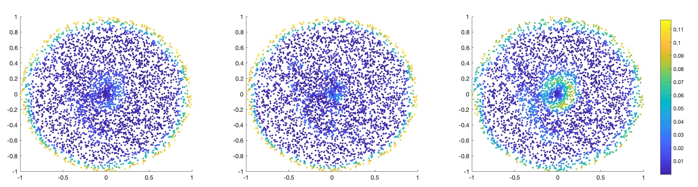
Figure 1. The plots of the BI constructed over $4000$ non-uniformly sampled points on the unit disc. Left Panel: The BI is constructed in the $\epsilon$-radius ball scheme with $\epsilon=0.2$, and the regularizer $c$ is chosen as in (3.2). Middle Panel: The BI is constructed in the KNN scheme with $K=70$ and the regularizer $c$ is chosen as in (3.2). Right Panel: The BI is constructed in the $\epsilon$-radius ball scheme with $\epsilon=0.2$ and the regularizer $c=\frac{1}{n}\sum_{i=1}^{n}\lambda_{n,d}(z_{i})$. The values of the BI are large over some interior points. When the regularizer is too small such as $c=\frac{1}{n}\sum_{i=1}^{n}\lambda_{n,d+1}(z_{i})$, the BI is not stable.

4. Theoretical Analysis

In this section, we delve into the theoretical analyses of the BI and the local covariance matrix, which are closely related. We present these analyses in both the $\epsilon$-radius ball scheme and the KNN scheme. To start, we provide an introduction of the essential geometric preliminaries.

4.1. Preliminary definitions

Suppose $g$ is the Riemannian metric on $M$. Denote $d_{g}(\cdot,\cdot)$ to be the distance function on $M$ associated with $g$. We define the following concepts around the boundary of $M$.

Definition 4.1.

1. Denote $x_{\partial}:=\arg\min_{y\in\partial M}d_{g}(y,x)$ and define the distance to the boundary function

   (4.1) $$\tilde{\epsilon}(x)=d_{g}(x,\partial M)=\min_{y\in\partial M}d_{g}(y,x).$$

   When $x\in M_{\epsilon}$ and $\epsilon$ is sufficiently small, due to the smoothness of the boundary, such $x_{\partial}$ is unique and we have $0\leq\tilde{\epsilon}(x)\leq\epsilon$.

2. For $\epsilon>0$, we define the $\epsilon$-neighborhood of $\partial M$ as

   $$M_{\epsilon}=\{x\in M|d_{g}(x,\partial M)<\epsilon\}.$$

3. For any $x\in\partial M$, let $\gamma_{x}(t)$ be the unit speed geodesic such that $\gamma_{x}(0)=x$ and $\gamma\,^{\prime}_{x}(0)$ is the unit inward normal vector at $x$.

The distance to the boundary function $d_{g}(x,\partial M)$ satisfies the following properties.

Proposition 4.1.

Under Assumption 3.1, $d_{g}(x,\partial M)$ is a continuous function on $M$ and differentiable almost everywhere on $M$. In particular, when $\epsilon$ is small enough, $d_{g}(x,\partial M)$ is smooth on $M_{\epsilon}$.

Recall that both the BI and the local covariance matrix are invariant under translation. Moreover, the BI is invariant under orthogonal transformation. Hence, we introduce the following assumption to simplify the proofs and the statements of of the main results.

Assumption 4.1.

For each fixed $x_{k}$, we translate and rotate $\iota(M)$ in $\mathbb{R}^{p}$ as follows.

1. We translate $\iota(M)$ in $\mathbb{R}^{p}$ so that $\iota(x_{k})=0$.

2. Denote $\{e_{i}\}_{i=1}^{p}$ to be the canonical basis of $\mathbb{R}^{p}$, where $e_{i}$ is a unit vector with $1$ in the $i$-th entry. Denote $\iota_{*}T_{x}M$ to be the embedded tangent space of $\iota(M)$ at $\iota(x)$ in $\mathbb{R}^{p}$ and $(\iota_{*}T_{x}M)^{\bot}$ be the normal space at $\iota(x)$. Fix any $\iota(x_{k})=0\in\iota(M)$, we assume that $\iota(M)$ has been properly rotated so that $\iota_{*}T_{x_{k}}M$ is spanned by $e_{1},\ldots,e_{d}$.

3. When $x_{k}\in M_{\epsilon}$ and $\epsilon$ is sufficiently small, let $x_{\partial,k}$ be the unique point on $\partial M$ which realizes the distance from $x_{k}$ to $\partial M$ defined in (1) of Definition 4.1. $\gamma_{x_{\partial,k}}(t)$ is the unit speed geodesic with $\gamma_{x_{\partial,k}}(0)=x_{\partial,k}$ and $\gamma_{x_{\partial,k}}(\tilde{\epsilon}(x_{k}))=x_{k}$. We further rotate $\iota(M)$ so that

   $$e_{d}=\iota_{*}\frac{d}{dt}\gamma_{x_{\partial,k}}(\tilde{\epsilon}(x_{k})).$$

   In particular, when $x\in\partial M$, $e_{d}$ is the inward normal direction of $\partial\iota(M)$ at $\iota(x)$.

At last, we introduce the following functions that will be used in the main results.

Definition 4.2.

Let $|S^{m}|$ denote the volume of the $m$ dimensional unit sphere. We define the following functions on $[0,\infty)$, where the constant $\frac{|S^{d-2}|}{d-1}$ is defined to be $1$ when $d=1$.

$$\sigma_{0}(t,\epsilon) :=\left\{\begin{array}[]{ll}\frac{|S^{d-1}|}{2d}+\frac{|S^{d-2}|}{d-1}\int_{0}^{\frac{t}{\epsilon}}(1-x^{2})^{\frac{d-1}{2}}dx&\mbox{ for }0\leq t\leq\epsilon\\ \frac{|S^{d-1}|}{d}&\mbox{ for }t>\epsilon\end{array}\right.$$

$$\sigma_{1,d}(t,\epsilon) :=\left\{\begin{array}[]{ll}-\frac{|S^{d-2}|}{d^{2}-1}(1-(\frac{t}{\epsilon})^{2})^{\frac{d+1}{2}}&\mbox{ for }0\leq t\leq\epsilon\\ 0&\mbox{ otherwise}\end{array}\right.$$

$$\sigma_{2}(t,\epsilon) :=\left\{\begin{array}[]{ll}\frac{|S^{d-1}|}{2d(d+2)}+\frac{|S^{d-2}|}{d^{2}-1}\int_{0}^{\frac{t}{\epsilon}}(1-x^{2})^{\frac{d+1}{2}}dx&\mbox{ for }0\leq t\leq\epsilon\\ \frac{|S^{d-1}|}{d(d+2)}&\mbox{ otherwise}\end{array}\right.$$

$$\sigma_{2,d}(t,\epsilon) :=\left\{\begin{array}[]{ll}\frac{|S^{d-1}|}{2d(d+2)}+\frac{|S^{d-2}|}{d-1}\int_{0}^{\frac{t}{\epsilon}}(1-x^{2})^{\frac{d-1}{2}}x^{2}dx&\mbox{ for }0\leq t\leq\epsilon\\ \frac{|S^{d-1}|}{d(d+2)}&\mbox{ otherwise}\end{array}\right.$$

$$\sigma_{3}(t,\epsilon) :=\left\{\begin{array}[]{ll}-\frac{|S^{d-2}|}{(d^{2}-1)(d+3)}(1-(\frac{t}{\epsilon})^{2})^{\frac{d+3}{2}}&\mbox{ for }0\leq t\leq\epsilon\\ 0&\mbox{ otherwise}\end{array}\right.$$

$$\sigma_{3,d}(t,\epsilon) :=\left\{\begin{array}[]{ll}-\frac{|S^{d-2}|}{(d^{2}-1)(d+3)}(2+(d+1)(\frac{t}{\epsilon})^{2})(1-(\frac{t}{\epsilon})^{2})^{\frac{d+1}{2}}&\mbox{ for }0\leq t\leq\epsilon\\ 0&\mbox{ otherwise}\end{array}\right.$$

Note that the functions $\sigma_{1,d}(t,\epsilon)$, $\sigma_{3}(t,\epsilon),$and $\sigma_{3,d}(t,\epsilon)$ are bounded from below by $0$ and above by constants depending on $d$. The functions $\sigma_{0}(t,\epsilon)$, $\sigma_{2}(t,\epsilon)$, and $\sigma_{2,d}(t,\epsilon)$ are bounded from below and above by constants depending on $d$. These functions are smooth everywhere except at $t=\epsilon$. At $t=\epsilon$, they are continuous and their level of smoothness depends on $d$.

4.2. Analyses of the local covariance matrix and the boundary indicator in the $\epsilon$-radius ball scheme

We provide the bias and variance analysis of the local covariance matrix in the $\epsilon$-radius ball scheme. The proof of the theorem is a combination of Lemma 31 and Lemma 37 in [28].

Theorem 4.1.

Under Assumptions 3.1, 3.2, and 4.1, let $\frac{1}{n}C_{n,k}$ be the local covariance matrix at $z_{k}$ constructed in the $\epsilon$-radius ball scheme, where $C_{n,k}$ is defined in (2.7). Suppose $\epsilon=\epsilon(n)$ such that $\frac{\sqrt{\log(n)}}{n^{1/2}\epsilon^{d/2+1}}\to 0$ and $\epsilon\to 0$ as $n\to\infty$. We have with probability greater than $1-n^{-2}$ that for all $k=1,\ldots,n$,

$$\frac{1}{n\epsilon^{d+2}}C_{n,k}=P(x_{k}){\begin{bmatrix}M^{(0)}(x_{k},\epsilon)&0\\ 0&0\end{bmatrix}}+{\begin{bmatrix}M^{(11)}(x_{k},\epsilon)&M^{(12)}(x_{k},\epsilon)\\ M^{(21)}(x_{k},\epsilon)&0\end{bmatrix}}\epsilon+O(\epsilon^{2})+O\Big{(}\frac{\sqrt{\log(n)}}{n^{1/2}\epsilon^{d/2}}\Big{)}.$$

The block matrices in the above expression satisfy the following properties.

1. $M^{(0)}(x,\epsilon)\in\mathbb{R}^{d\times d}$ is a diagonal matrix. The $i$th diagonal entry is $\sigma_{2}(\tilde{\epsilon}(x_{k}),\epsilon)$ for $1\leq i\leq d-1$ and the $d$th diagonal entry is $\sigma_{2,d}(\tilde{\epsilon}(x_{k}),\epsilon)$.

2. $M^{(11)}(x_{k},\epsilon)$ is symmetric and $M^{(12)}(x_{k},\epsilon)=M^{(21)}(x_{k},\epsilon)^{\top}$. The entries in $M^{(11)}(x_{k},\epsilon)$, $M^{(12)}(x_{k},\epsilon)$, and $M^{(21)}(x_{k},\epsilon)$ are $0$ when $x_{k}\in M\setminus M_{\epsilon}$.

3. For all $x_{k}$, the magnitude of the entries in $M^{(11)}(x_{k},\epsilon)$, $M^{(12)}(x_{k},\epsilon)$, and $M^{(21)}(x_{k},\epsilon)$ can be bounded from above by a constant depending on $d$, the $C^{1}$ norm of $P$, the second fundamental form of $\iota(M)$ in $\mathbb{R}^{p}$ at $\iota(x_{k})$, and the second fundamental form of $\partial M$ in $M$ at $x_{\partial,k}$.

4. $O(\epsilon^{2})$ and $O\Big{(}\frac{\sqrt{\log(n)}}{n^{1/2}\epsilon^{d/2}}\Big{)}$ represent $p\times p$ matrices whose entries are of orders $O(\epsilon^{2})$ and $O\Big{(}\frac{\sqrt{\log(n)}}{n^{1/2}\epsilon^{d/2}}\Big{)}$ respectively.

Under the assumptions in the above theorem, suppose $\epsilon=\epsilon(n)$ such that $\frac{\sqrt{\log(n)}}{n^{1/2}\epsilon^{d/2+1}}\to 0$ and $\epsilon\to 0$ as $n\to\infty$. The above theorem implies that with probability greater than $1-n^{-2}$, for all $x_{k}\in M\setminus M_{\epsilon}$,

$$\frac{1}{n\epsilon^{d+2}}C_{n,k}=\frac{P(x)|S^{d-1}|}{d(d+2)}{\begin{bmatrix}I_{d\times d}&0\\ 0&0\end{bmatrix}}+O(\epsilon^{2})+O\Big{(}\frac{\sqrt{\log(n)}}{n^{1/2}\epsilon^{d/2}}\Big{)}.$$

This result matches the analysis of the local covariance matrix constructed from samples on a closed manifold.

Since the eigenvalues $\{\lambda_{n,i}(z_{k})\}_{i=1}^{p}$ of $C_{n,k}$ are invariant under translation of $\mathcal{X}$ and orthogonal transformation on $\mathbb{R}^{p}$. By applying a perturbation argument (Appendix A in [26]), for all $k$

$$\frac{\lambda_{n,i}(z_{k})}{n}=P(x_{k})\sigma_{2}(\tilde{\epsilon}(x_{k}),\epsilon)\epsilon^{d+2}+O(\epsilon^{d+3})+O\Big{(}\sqrt{\frac{\log(n)}{n}}\epsilon^{d/2+2}\Big{)}\quad \text{for $i=1,\cdots,d-1$};$$

$$\frac{\lambda_{n,i}(z_{k})}{n}=P(x_{k})\sigma_{2,d}(\tilde{\epsilon}(x_{k}),\epsilon)\epsilon^{d+2}+O(\epsilon^{d+3})+O\Big{(}\sqrt{\frac{\log(n)}{n}}\epsilon^{d/2+2}\Big{)} \text{for $i=d$};$$

$$\frac{\lambda_{n,i}(z_{k})}{n}=O(\epsilon^{d+4})+O\Big{(}\sqrt{\frac{\log(n)}{n}}\epsilon^{d/2+2}\Big{)} \text{for $i=d+1,\cdots p$}.$$

Suppose $U_{n,k}\in O(p)$ is the corresponding orthonormal eigenvector matrix of $C_{n,k}$. Suppose $X_{k,1}\in O(d)$ and $X_{k,2}\in O(p-d)$. If $x_{k}\in M_{\epsilon}$, then

$$U_{n,k}=\begin{bmatrix}X_{k,1}&0\\ 0&X_{k,2}\end{bmatrix}+O(\epsilon)+O\Big{(}\frac{\sqrt{\log(n)}}{n^{1/2}\epsilon^{d/2}}\Big{)}.$$

If $x_{k}\in M\setminus M_{\epsilon}$, then

$$U_{n,k}=\begin{bmatrix}X_{k,1}&0\\ 0&X_{k,2}\end{bmatrix}+O(\epsilon^{2})+O\Big{(}\frac{\sqrt{\log(n)}}{n^{1/2}\epsilon^{d/2}}\Big{)}.$$

Since we propose Assumption 4.1, $\begin{bmatrix}X_{k,1}\\ 0\end{bmatrix}$ forms an orthonormal basis of $\iota_{*}T_{x_{k}}M$, and $\begin{bmatrix}0\\ X_{k,2}\end{bmatrix}$ forms an orthonormal basis of $(\iota_{*}T_{x_{k}}M)^{\bot}$. Therefore, when $x_{k}\in M_{\epsilon}$, an orthonormal basis of $\iota_{*}T_{x_{k}}M$ can be approximated by $U_{n,k}\begin{bmatrix}I_{d\times d}\\ 0_{(p-d)\times d}\end{bmatrix}$, up to a matrix whose entries are of order $O(\epsilon)+O\Big{(}\frac{\sqrt{\log(n)}}{n^{1/2}\epsilon^{d/2}}\Big{)}$.

Next, we provide the following bias and variance analysis of the BI under the $\epsilon$-radius ball scheme. The proof of the theorem is in Section A of the Supplementary Material.

Theorem 4.2.

Under Assumptions 3.1, 3.2, 4.1, and the $\epsilon$-radius ball scheme, suppose the regularizer $c=n\epsilon^{d+3}$ and suppose $\epsilon=\epsilon(n)$ so that $\frac{\sqrt{\log(n)}}{n^{1/2}\epsilon^{d/2+1}}\to 0$ and $\epsilon\to 0$ as $n\to\infty$. When $\epsilon$ is small enough, with probability greater than $1-2n^{-2}$, for all $k=1,\ldots,n$,

$$B_{k}=B(x_{k})+O(\epsilon)+O\Big{(}\frac{\sqrt{\log(n)}}{n^{1/2}\epsilon^{d/2}}\Big{)}\,,$$

where the constants in $O(\epsilon)$ and $O\Big{(}\frac{\sqrt{\log(n)}}{n^{1/2}\epsilon^{d/2}}\Big{)}$ depend on $P_{m}$, the $C^{1}$ norm of $P$ and the second fundamental form of $\iota(M)$.

The function $B(x):M\to\mathbb{R}$ has the following properties:

1. $B(x)=\frac{(\sigma_{1,d}(\tilde{\epsilon}(x),\epsilon))^{2}}{\sigma_{0}(\tilde{\epsilon}(x),\epsilon)\sigma_{2,d}(\tilde{\epsilon}(x),\epsilon)}$. Hence, $B(x)$ is always continuous on $M$. When $\epsilon$ is small enough, it is smooth except at the set $\{x\in M|d_{g}(x,\partial M)=\epsilon\}$.

2. $B(x)=\frac{4d^{2}(d+2)|S^{d-2}|^{2}}{(d^{2}-1)^{2}|S^{d-1}|^{2}}$ when $x\in\partial M$.

3. $B(x)=0$ when $x\in M\setminus M_{\epsilon}$.

4. For $x_{1},x_{2}\in\partial M$, $B(\gamma_{x_{1}}(t))=B(\gamma_{x_{2}}(t))$ for $0\leq t\leq\epsilon$.

5. Fix any $x\in\partial M$, $B(\gamma_{x}(t))$ is a monotone decreasing function of $t$ for $0\leq t\leq\epsilon$. Moreover $\frac{d^{2}(d+2)|S^{d-2}|^{2}}{(d^{2}-1)^{2}|S^{d-1}|^{2}}(1-(\frac{t}{\epsilon})^{2})^{d+1}\leq B(\gamma_{x}(t))\leq\frac{4d^{2}(d+2)|S^{d-2}|^{2}}{(d^{2}-1)^{2}|S^{d-1}|^{2}}(1-(\frac{t}{\epsilon})^{2})^{d+1}$ for $0\leq t\leq\epsilon$.

6. For any $0<\tau<\frac{4d^{2}(d+2)|S^{d-2}|^{2}}{(d^{2}-1)^{2}|S^{d-1}|^{2}}$, $B^{-1}(\tau,\infty)=M_{r}$ with $M_{r}\subset M_{\epsilon}$.

We discuss the implications of the above results regarding the BI in the $\epsilon$-radius ball scheme. By (2) and (4), $B(x)$ remains constant and attains maximum on $\partial M$. Additionally, (4) and (5) indicate that $B(x)$ decreases monotonically at the same speed along any geodesic perpendicular to $\partial M$. Therefore, according to (3), the function $B(x)$ behaves like a bump function, concentrating on $\partial M$ and vanishing in $M\setminus M_{\epsilon}$.

Suppose $\epsilon$ and $n$ satisfy the conditions in Theorem 4.2. For $n$ large enough, with high probability, we have $|B_{k}-B(x_{k})|=O(\epsilon)$. Thus, when $x_{k}$ is near the boundary, $B_{k}$ approximates an order $1$ constant. Specifically, from (3.1), we have $B_{k}=\frac{\bm{1}_{N_{k}}^{\top}G_{n,k}^{\top}\mathcal{I}_{c}(C_{n,k})G_{n,k}\bm{1}_{N_{k}}}{N_{k}}$. The denominator $N_{k}$ acts like the $0-1$ kernel density estimator, eliminating the impact of the non-uniform distribution of the samples and ensuring that $B_{k}$ remains close to a constant near the boundary. Refer to Lemma A.2 in Section A of the Supplementary Material for a detailed discussion. Additionally, refer to Proposition A.1 in Section A of the Supplementary Material for a strong uniform consistency result of kernel density estimation through $0-1$ kernel on a manifold with boundary. When $x_{k}\in M\setminus M_{\epsilon}$, $B_{k}$ is of order $O(\epsilon)$. Therefore, by (6), we can select a threshold on $B_{k}$ to identify points in $\iota(M_{r})$ for some $M_{r}\subset M_{\epsilon}$. Moreover, according to the conditions in Theorem 4.2, choosing a smaller $\epsilon$ for larger $n$ reduces the error between $B_{k}$ and $B(x_{k})$ and decreases the size of $M_{\epsilon}$. In conclusion, larger $n$ enables more accurate detection of boundary points.

4.3. Analyses of the boundary indicator and the local covariance matrix in the KNN scheme

We start with the following definition.

Definition 4.3.

Let $B_{a}^{\mathbb{R}^{p}}(z)$ be the $p$ dimensional closed ball of radius $a$ centered at $z$ in $\mathbb{R}^{p}$. For any $x\in M$, define $N_{a}(x)=|B_{a}^{\mathbb{R}^{p}}(\iota(x))\cap\mathcal{X}|$. We define the following radius at $x$ associated with $K$:

$$R(x)=\inf_{a}\{a>0,N_{a}(x)\geq K+1\}.$$

Then, $R(x)$ has the following properties. The proof of the proposition is in Section B of the Supplementary Material.

Proposition 4.2.

1. $R(x)$ is a continuous function on $M$.

2. For any $x\in\partial M$, suppose $\gamma_{x}(t)$ is minimizing on $[0,t_{2}]$. Then $R(x)$ is Lipschitz along $\gamma_{x}(t)$ for $0\leq t\leq t_{2}$. Specifically, if $t_{1}<t_{2}$, then $|R(\gamma_{x}(t_{1}))-R(\gamma_{x}(t_{2}))|\leq t_{2}-t_{1}$. Moreover, $\frac{t_{1}}{R(\gamma_{x}(t_{1}))}<\frac{t_{2}}{R(\gamma_{x}(t_{2}))}$ whenever $t_{1}<R(\gamma_{x}(t_{1}))$.

Since $R(x)$ is a continuous function on $M$ and $M$ is compact, $R(x)$ attains a maximum with

$$R^{*}=\max_{x\in M}R(x).$$

Recall the function $\sigma_{0}$ in Definition 4.2. For a fixed $t\geq 0$, let

$$V(t,r)=\sigma_{0}(t,r)r^{d}.$$

Let $(x_{1},x_{2},\cdots,x_{d})$ denote the coordinates in $\mathbb{R}^{d}$. The function $V(t,r)$ represents the volume of the region $\mathcal{R}_{t,r}$ between the ball of radius $r$ centered at the origin in $\mathbb{R}^{d}$ and the hyperplane $x_{d}=t$. Specifically, when $r\leq t$, $V(t,r)=\frac{|S^{d-1}|}{d}r^{d}$ is the volume of the ball of radius $r$. Note that $V(t,r):[0,\infty)\rightarrow[0,\infty)$ is a continuous, monotone increasing function of $r$ for a fixed $t$, and $V(t,r)$ is differentiable except at $r=t$. Hence, $s=V(t,r)$ has an inverse $r=U(t,s)$, where $U(t,s):[0,\infty)\rightarrow[0,\infty)$ is also monotone increasing. Specifically, $U(t,s)=(\frac{ds}{|S^{d-1}|})^{\frac{1}{d}}$ for $s<\frac{|S^{d-1}|}{d}t^{d}$. Moreover, by the inverse function theorem, $U(t,s)$ is differentiable everywhere except at $s=0$ for $d>1$ and at $s=\frac{|S^{d-1}|}{d}t^{d}$. Suppose $\tilde{\epsilon}(x)$ is the distance from $x\in M$ to $\partial M$ as defined in (4.1). Let

$$\tilde{R}(x)=U(\tilde{\epsilon}(x),\frac{K+1}{P(x)n}).$$

We show that $\tilde{R}(x)$ is an estimator of $R(x)$. The proof of the proposition is in Section B of the Supplementary Material.

Proposition 4.3.

Suppose we have $\frac{K}{n}\rightarrow 0$ and $\frac{\log(n)}{K}(\frac{n}{K})^{2/d}\to 0$ as $n\to\infty$. Then, for all $x\in M$, with probability greater than $1-2n^{-2}$, we have $R(x)=\tilde{R}(x)(1+O((\frac{K}{n})^{\frac{1}{d}}))$, where the constant in $O((\frac{K}{n})^{\frac{1}{d}})$ depends on $d$, $C^{1}$ norm of $P$, and $P_{m}$. Moreover,

$$\frac{1}{2}(\frac{d}{|S^{d-1}|})^{\frac{1}{d}}(\frac{K}{P_{M}n})^{\frac{1}{d}}\leq R^{*}\leq 3(\frac{2d}{|S^{d-1}|})^{\frac{1}{d}}(\frac{K}{P_{m}n})^{\frac{1}{d}}$$

.

Observe that for any $z_{k}\in\mathcal{X}$, $C_{n,k}$ constructed through the KNN scheme is equal to the $C_{n,k}$ constructed through the $R(x_{k})$-radius ball scheme. Hence, by applying Proposition 4.3 and Theorem 4.1, we provide the bias and variance analysis of the local covariance matrix in the KNN scheme. The proof of theorem is in Section C of the Supplementary Material.

Theorem 4.3.

Under Assumptions 3.1, 3.2, and 4.1, let $\frac{1}{n}C_{n,k}$ be the local covariance matrix at $z_{k}$ constructed in the KNN scheme, where $C_{n,k}$ is defined in (2.7). Suppose $K=K(n)$ so that $\frac{K}{n}\rightarrow 0$ and $\frac{\log(n)}{K}(\frac{n}{K})^{2/d}\to 0$ as $n\to\infty$. Then, with probability greater than $1-4n^{-2}$, for all $k$,

$$\frac{1}{n}C_{n,k}={\begin{bmatrix}\tilde{M}^{(0)}(x_{k})&0\\ 0&0\end{bmatrix}}+\begin{bmatrix}\tilde{M}^{(11)}(x_{k},\frac{K}{n})&\tilde{M}^{(12)}(x_{k},\frac{K}{n})\\ \tilde{M}^{(21)}(x_{k},\frac{K}{n})&0\end{bmatrix}+O((\frac{K}{n})^{\frac{d+4}{d}})+O\Big{(}\frac{\sqrt{K\log(n)}}{n}(\frac{K}{n})^{\frac{2}{d}}\Big{)}.$$

The properties of the block matrices are summarized as follows.

1. For $x\in M$, $\tilde{M}^{(0)}(x)\in\mathbb{R}^{d\times d}$ is a diagonal matrix.

   1. The $i$th diagonal entry of $\tilde{M}^{(0)}(x)$ is $\mu_{1}(x)+O((\frac{K}{n})^{\frac{d+3}{d}})$, for $i=1,\cdots,d-1$. The $d$th diagonal entry of $\tilde{M}^{(0)}(x)$ is $\mu_{2}(x)+O((\frac{K}{n})^{\frac{d+3}{d}})$.

   2. $\mu_{1}(x)$ and $\mu_{2}(x)$ are continuous functions on $M$. For all $x\in M$,

      $$\frac{1}{2(d+2)}(\frac{d}{|S^{d-1}|P_{M}})^{\frac{2}{d}}(\frac{K+1}{n})^{\frac{d+2}{d}}\leq\mu_{1}(x),\mu_{2}(x)\leq\frac{2}{d+2}(\frac{2d}{|S^{d-1}|P_{m}})^{\frac{2}{d}}(\frac{K+1}{n})^{\frac{d+2}{d}}.$$

   3. When $x\in\partial M$,

      $$\mu_{1}(x)=\mu_{2}(x)=\frac{1}{(d+2)}(\frac{2d}{|S^{d-1}|P(x)})^{\frac{2}{d}}(\frac{K+1}{n})^{\frac{d+2}{d}}.$$

2. $\tilde{M}^{(11)}(x_{k},\frac{K}{n})$ is symmetric and $\tilde{M}^{(12)}(x_{k},\frac{K}{n})=\tilde{M}^{(21)}(x_{k},\frac{K}{n})^{\top}$. The entries in those matrices are of order $O((\frac{K}{n})^{\frac{d+3}{d}})$, where the constant in $O((\frac{K}{n})^{\frac{d+3}{d}})$ depends on $d$, $P_{m}$, the $C^{1}$ norm of $P$, the second fundamental form of $\iota(M)$ in $\mathbb{R}^{p}$ at $\iota(x_{k})$, and the second fundamental form of $\partial M$ in $M$ at $x_{\partial,k}$.

3. For $x_{k}\in M\setminus M_{R^{*}}$,

   $$\frac{1}{n}C_{n,k}={\begin{bmatrix}\tilde{M}^{(0)}(x_{k})&0\\ 0&0\end{bmatrix}}+O((\frac{K}{n})^{\frac{d+4}{d}})+O\Big{(}\frac{\sqrt{K\log(n)}}{n}(\frac{K}{n})^{\frac{2}{d}}\Big{)}.$$

   The $i$th diagonal entry of $\tilde{M}^{(0)}(x_{k})$ is $\frac{1}{(d+2)}(\frac{d}{|S^{d-1}|P(x_{k})})^{\frac{2}{d}}(\frac{K+1}{n})^{\frac{d+2}{d}}+O((\frac{K}{n})^{\frac{d+3}{d}}),$ for $1\leq i\leq d$.

4. $O((\frac{K}{n})^{\frac{d+4}{d}})$ and $O\Big{(}\frac{\sqrt{K\log(n)}}{n}(\frac{K}{n})^{\frac{2}{d}}\Big{)}$ represent $p\times p$ matrices whose entries are of orders $O((\frac{K}{n})^{\frac{d+4}{d}})$ and $O\Big{(}\frac{\sqrt{K\log(n)}}{n}(\frac{K}{n})^{\frac{2}{d}}\Big{)}$ respectively.

Similar to the discussion of the spectral properties of $C_{n,k}$ in the $\epsilon$-radius scheme, based on the above theorem, the eigenvalues $\{\lambda_{n,i}(z_{k})\}_{i=1}^{p}$ of $C_{n,k}$ constructed in the KNN scheme can be characterized as follows. For all $k$,

$$\frac{\lambda_{n,i}(z_{k})}{n}=\mu_{1}(x_{k})+O((\frac{K}{n})^{\frac{d+3}{d}})+O\Big{(}\frac{\sqrt{K\log(n)}}{n}(\frac{K}{n})^{\frac{2}{d}}\Big{)} \text{for $i=1,\cdots,d-1$};$$

$$\frac{\lambda_{n,i}(z_{k})}{n}=\mu_{2}(x_{k})+O((\frac{K}{n})^{\frac{d+3}{d}})+O\Big{(}\frac{\sqrt{K\log(n)}}{n}(\frac{K}{n})^{\frac{2}{d}}\Big{)} \text{for $i=d$};$$

$$\frac{\lambda_{n,i}(z_{k})}{n}=O((\frac{K}{n})^{\frac{d+4}{d}})+O\Big{(}\frac{\sqrt{K\log(n)}}{n}(\frac{K}{n})^{\frac{2}{d}}\Big{)} \text{for $i=d+1,\cdots p$}.$$

In particular, when $x_{k}\in M\setminus M_{R^{*}}$, $\mu_{1}(x_{k})=\mu_{2}(x_{k})=\frac{1}{(d+2)}(\frac{d}{|S^{d-1}|P(x_{k})})^{\frac{2}{d}}(\frac{K+1}{n})^{\frac{d+2}{d}}$.

Suppose $U_{n,k}\in O(p)$ is the corresponding orthonormal eigenvector matrix of $C_{n,k}$. Suppose $X_{k,1}\in O(d)$ and $X_{k,2}\in O(p-d)$. For any $k$,

$$U_{n,k}=\begin{bmatrix}X_{k,1}&0\\ 0&X_{k,2}\end{bmatrix}+O((\frac{K}{n})^{\frac{d+3}{d}})+O\Big{(}\frac{\sqrt{K\log(n)}}{n}(\frac{K}{n})^{\frac{2}{d}}\Big{)}.$$

If $x_{k}\in M\setminus M_{R^{*}}$, then

$$U_{n,k}=\begin{bmatrix}X_{k,1}&0\\ 0&X_{k,2}\end{bmatrix}+O((\frac{K}{n})^{\frac{d+4}{d}})+O\Big{(}\frac{\sqrt{K\log(n)}}{n}(\frac{K}{n})^{\frac{2}{d}}\Big{)}.$$

To end this subsection, we provide the following bias and variance analysis of the BI in the KNN scheme. The proof of the theorem is in Section C of the Supplementary Material.

Theorem 4.4.

Under Assumptions 3.1, 3.2, 4.1, and the KNN scheme, suppose $c=n(\frac{K}{n})^{\frac{d+3}{d}}$ and suppose $K=K(n)$ so that $\frac{K}{n}\rightarrow 0$ and $\frac{\log(n)}{K}(\frac{n}{K})^{2/d}\to 0$ as $n\to\infty$. Then, with probability greater than $1-4n^{-2}$, for all $k$,

$$B_{k}=\tilde{B}(x_{k})+O((\frac{K}{n})^{\frac{1}{d}})+O\Big{(}\sqrt{\frac{\log(n)}{K}}\Big{)},$$

The constants in $O((\frac{K}{n})^{\frac{1}{d}})$ and $O\Big{(}\sqrt{\frac{\log(n)}{K}}\Big{)}$ depend on $P_{m}$, the $C^{1}$ norm of $P$ and the second fundamental form of $\iota(M)$. The function $\tilde{B}(x):M\to\mathbb{R}$ has the following properties:

1. $\tilde{B}(x)$ is continuous on $M$.

2. Define $\frac{|S^{d-2}|}{d-1}=1$ when $d=1$. $\tilde{B}(x)=\frac{4d^{2}(d+2)|S^{d-2}|^{2}}{(d^{2}-1)^{2}|S^{d-1}|^{2}}$ when $x\in\partial M$.

3. If $n$ is large enough, then $R^{*}$ is small enough and $\gamma_{x}(t)$ is mimizing on $[0,2R^{*}]$ for all $x\in\partial M$. There exists $0<t_{x}^{*}<R^{*}$ with $\tilde{B}(\gamma_{x}(t))=0$ for $t\geq t_{x}^{*}$ and $\tilde{B}(\gamma_{x}(t))$ decreasing for $0<t<t_{x}^{*}$.

We discuss the implications of the above results concerning the BI in the KNN scheme. By (2) and (3), $\tilde{B}(x)$ remains constant and attains maximum on $\partial M$. Furthermore, for any point $x$ on $\partial M$, $\tilde{B}(\gamma_{x}(t))$ decreases along the geodesic $\gamma_{x}(t)$ from $x$ to $\tilde{B}(\gamma_{x}(t_{x}^{*}))$ and $\tilde{B}(\gamma_{x}(t))=0$ when $t\geq t_{x}^{*}$. Since $t_{x}^{*}<R^{*}$, the region where $\tilde{B}(x)$ is non zero is contained in $M_{R^{*}}$. Hence, $\tilde{B}(x)$ behaves like a bump function, concentrating on $\partial M$ and vanishing in $M\setminus M_{R^{*}}$. However, unlike $B(x)$ in the $\epsilon$-radius ball scheme, $\tilde{B}(x)$ in the KNN scheme may not decrease at the same speed along geodesics perpendicular to $\partial M$. Refer to Figure 2 for an illustration. If we choose $0<\tau<\frac{4d^{2}(d+2)|S^{d-2}|^{2}}{(d^{2}-1)^{2}|S^{d-1}|^{2}}$, $\tilde{B}^{-1}(\tau,\infty)=N_{\tau}$, where $N_{\tau}\subset M_{R^{*}}$ is a neighborhood of $\partial M$ in $M$.

Suppose $K$ and $n$ satisfy the conditions in Theorem 4.4. When $n$ is large enough, $\sqrt{\frac{\log(n)}{K}}\leq(\frac{K}{n})^{\frac{1}{d}}$. With high probability, we have $|B_{k}-\tilde{B}(x_{k})|=O((\frac{K}{n})^{\frac{1}{d}})$. Therefore, when $x_{k}$ is near the boundary, $B_{k}$ approximates a constant value, and within $M\setminus M_{R^{*}}$, $B_{k}$ is of order $O((\frac{K}{n})^{\frac{1}{d}})$. Thus, we can set a threshold on $B_{k}$ to identify all points in a neighborhood of the boundary contained in $M_{R^{*}}$. According to Proposition 4.3, as $n$ increases, $R^{*}$ deceases, leading to more precise identification of boundary points.

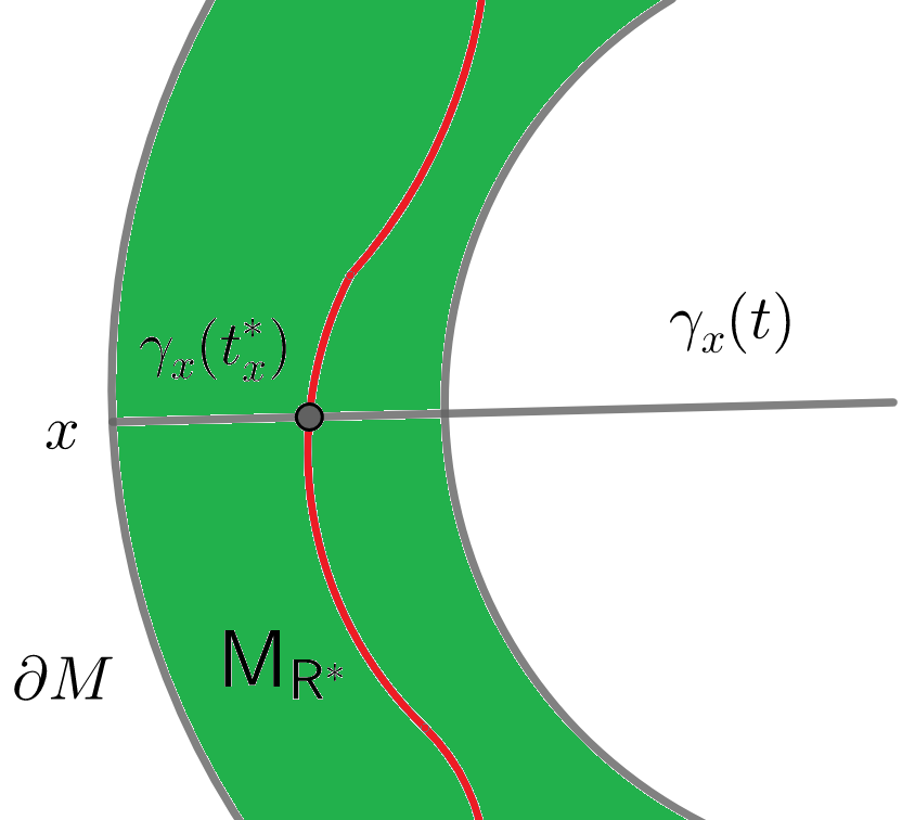
Figure 2. An illustration to the function $\tilde{B}(x)$ in the KNN scheme in a neighborhood near the boundary of $M$. The green region is the intersection of $M_{R^{*}}$ and the neighborhood. The red curve is the union of $\gamma_{x}(t_{x}^{*})$ corresponding to all $x\in\partial M$. For any $x\in\partial M$, $\tilde{B}(\gamma_{x}(t))$ decreases along the geodesic $\gamma_{x}(t)$ from $x$ to $\tilde{B}(\gamma_{x}(t_{x}^{*}))$ and $\tilde{B}(\gamma_{x}(t))=0$ when $t\geq t_{x}^{*}$. Since $t_{x}^{*}\leq R^{*}$, $\tilde{B}=0$ on $M\setminus M_{R^{*}}$.

5. Numerical results

In this section, we compare the performances of BD-LLE in three examples with different boundary detection algorithms including $\alpha$-shape [13, 14], BAND [30], BORDER [29], BRIM [19], LEVER [7], SPINVER [20], and the CPS algorithm [5](abbreviated by authors’ initials for brevity). Note that all algorithms, except $\alpha$-shape, require either the $\epsilon$-radius ball scheme or the KNN scheme for nearest neighborhood search. For $\alpha$-shape, we apply the boundary function in MATLAB, which includes a shrink factor $s\in[0,1]$ corresponding to $\alpha$. Detailed descriptions of all the algorithm are summarized in Section D of the Supplementary Material, where each algorithm is presented along with the notations and setups used in this work.

We introduce the following method to evaluate the performance of a boundary detection algorithm. Suppose we fix the scale parameter, $\epsilon$ or $K$, for an algorithm. Let $\partial\mathcal{X}$ denote the boundary points detected from $\mathcal{X}$. Let $M_{r}$ represent the $r$-neighborhood of $\partial M$ as defined in Definition 4.1. We define the $F1$ score of $\partial\mathcal{X}$ associated with $r$ as follows:

$$\text{F}1(\partial\mathcal{X},r)=\frac{2}{\frac{1}{\frac{|\partial\mathcal{X}\cap\iota(M_{r})|}{|\partial\mathcal{X}|}}+\frac{1}{\frac{|\partial\mathcal{X}\cap\iota(M_{r})|}{|\mathcal{X}\cap\iota(M_{r})|}}}=\frac{2|\partial\mathcal{X}\cap\iota(M_{r})|}{|\partial\mathcal{X}|+|\mathcal{X}\cap\iota(M_{r})|}$$

Since $\partial M$ is a measure $0$ subset of $M$, based on Assumption 3.2, the probability for a sample in $\mathcal{X}$ to lie on the boundary of $\iota(M)$ is $0$. Therefore, our objective is to determine whether the detected boundary points $\partial\mathcal{X}$ coincide with the points within some regular neighborhood of the boundary, e.g. the $r$-neighborhood. We propose the metric $F1_{max}$, defined as the maximum $F1$ score over a sequence $\{r_{i}=0.05i\}_{i=1}^{k}$, i.e. $F1_{max}=\max_{1\leq i\leq k}F1(\partial\mathcal{X},r_{i})$.

Note that unlike other algorithms, the CPS algorithm detects the boundary points through directly estimating the distance to the boundary function. In other words, for $z_{k}\in\mathcal{X}$ close to the boundary, $d_{g}(\iota^{-1}(z_{k}),\partial M)$ is estimated. By introducing an additional parameter $r$ alongside the scale parameter, the algorithm outputs $\partial\mathcal{X}(r)$ which estimates $\mathcal{X}\cap\iota(M_{r})$. Therefore, for a given sequence $\{r_{i}=0.05i\}_{i=1}^{k}$, we apply the CPS algorithm to output the corresponding $\partial\mathcal{X}(r_{i})$, and we define $F1_{max}=\max_{1\leq i\leq k}F1(\partial\mathcal{X}(r_{i}),r_{i})$.

Next, we describe the construction of the point cloud for each example.

5.1. Unit disc

We uniformly randomly sample $\{s_{i}\}_{j=1}^{10^{4}}$ and $\{t_{j}\}_{j=1}^{10^{4}}$ from $[0,1]$ respectively. Let $\mathcal{Y}=\{\tilde{z}_{j}=(x_{j},y_{j})\}_{j=1}^{10^{4}}\subset\mathbb{R}^{2}$ where $x_{j}=\exp{(\frac{-s_{j}^{2}}{s_{j}^{2}+1})}$ and $y_{j}=\exp{(\frac{-t_{j}^{2}}{t_{j}^{2}+1})}$. $\mathcal{X}\subset\mathbb{R}^{2}$ consists of $4171$ points from $\mathcal{Y}$ such that if $\|\tilde{z}_{j}\|_{\mathbb{R}^{2}}\leq 1$, then $\tilde{z}_{j}\in\mathcal{X}$. Thus, we generate $4171$ non-uniform samples $\mathcal{X}=\{z_{i}\}_{i=1}^{4171}$ on the unit disc. We apply BD-LLE in the $\epsilon$-radius ball scheme to $\mathcal{X}$ with $\epsilon=0.15$. We summarize the scale parameters used in other algorithms in Table 2, and $F1_{\max}$ for all the algorithms in Table 3. We plot $\mathcal{X}$ and the detected boundary points $\partial\mathcal{X}$ for each algorithm in Figure 3.

Table 2. Summary of the nearest neighborhood search schemes and the scale parameters in different algorithms .

Algorithms	Nearest neighborhood	Unit disc	Vertical-cut torus	Tilted-cut torus
BD-LLE	$\epsilon$-radius ball	$\epsilon=0.15$	$\epsilon=1$	$\epsilon=1.25$
$\alpha$-shape	Shrink factor	1	0	0
BAND	KNN	K=50	K=50	K=50
BORDER	KNN	K=50	K=50	K=50
BRIM	$\epsilon$-radius ball	$\epsilon=0.15$	$\epsilon=1$	$\epsilon=1.25$
CPS	$\epsilon$-radius ball	$\epsilon=0.15$	$\epsilon=1$	$\epsilon=0.8$
LEVER	KNN	K=50	K=50	K=50
SPINVER	KNN	K=50	K=50	K=50

Table 3. Summary of $F1_{max}$ for all the algorithms. The largest $F1_{max}$ in each example is highlighted.

Algorithms	Unit disc	Vertical-cut torus	Tilted-cut torus
BD-LLE	0.8814	0.9344	0.8356
$\alpha$-shape	0.7129	0.1511	0.2096
BAND	0.1289	0.3679	0.3491
BORDER	0.4754	0.4895	0.3833
BRIM	0.6969	0.1238	0.1073
CPS	0.8867	0.9022	0.8000
LEVER	0.4020	0.6679	0.5609
SPINVER	0.3705	0.5607	0.3313

24

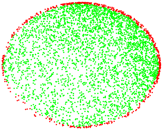
(a) BD-LLE

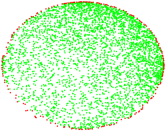
(b) $\alpha$-shape

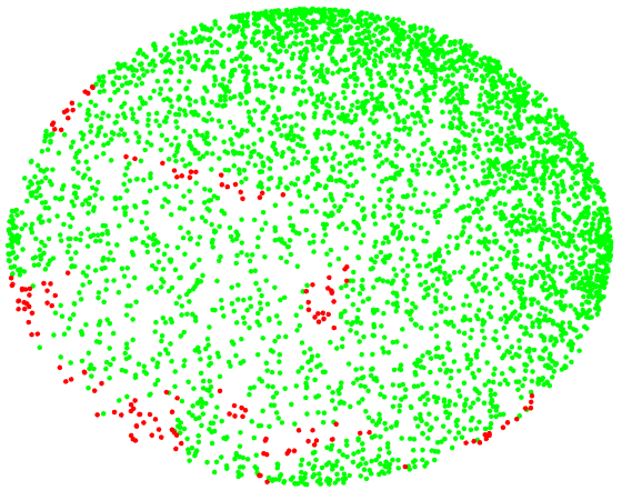
(c) BAND

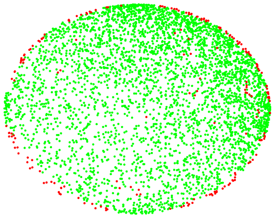
(d) BORDER

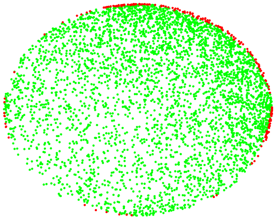
(e) BRIM

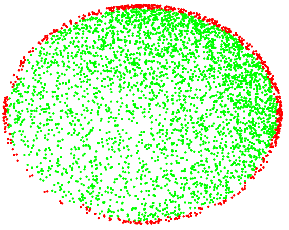
(f) CPS

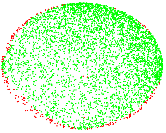
(g) LEVER

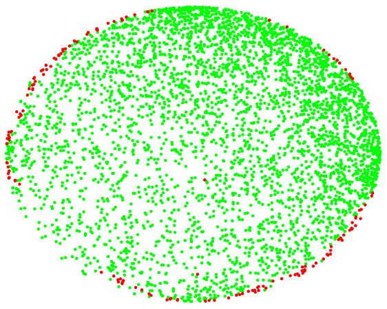
(h) SPINVER

Figure 3. The plot of $\mathcal{X}$ (green and red) and $\partial\mathcal{X}$ (red) for different algorithms in the unit disc example.

5.2. Vertical-cut torus

We uniformly randomly sample $\{\theta_{i}\}_{i=1}^{5056}$ and $\{\phi_{j}\}_{i=1}^{5056}$ from $[-\pi,\pi)$ and $[-\pi,\pi)\setminus(-0.5,0.5)$ respectively. Let $\mathcal{X}=\{z_{i}\}_{i=1}^{5056}\subset\mathbb{R}^{3}$, where

$$z_{i}=(3+1.2\cos(\theta_{i})\cos(\phi_{i}),3+1.2\cos(\theta_{i})\sin(\phi_{i}),1.2\sin(\theta_{i})).$$

Thus, we generate $5056$ non-uniform samples $\mathcal{X}=\{z_{i}\}_{i=1}^{5056}$ on the vertical-cut torus. We apply BD-LLE in the $\epsilon$-radius ball scheme to $\mathcal{X}$ with $\epsilon=1$. We summarize the scale parameters used in other algorithms in Table 2, and $F1_{\max}$ for all the algorithms in Table 3. We plot $\mathcal{X}$ and the detected boundary points $\partial\mathcal{X}$ for each algorithm in Figure 4.

24

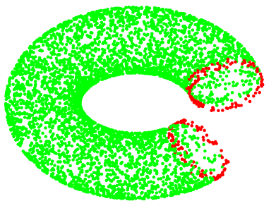
(a) BD-LLE

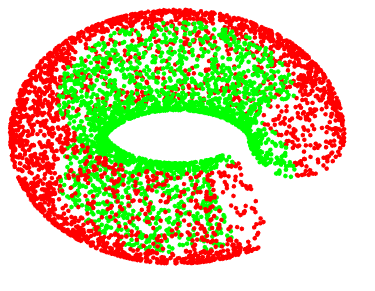
(b) $\alpha$-shape

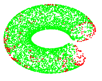
(c) BAND

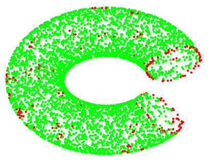
(d) BORDER

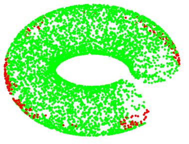
(e) BRIM

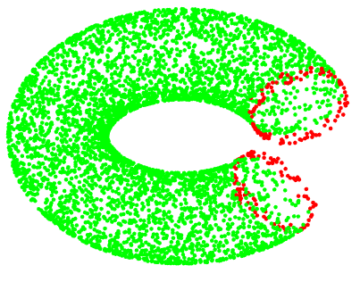
(f) CPS

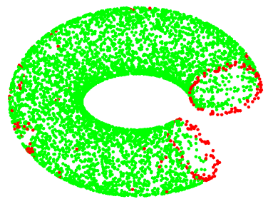
(g) LEVER

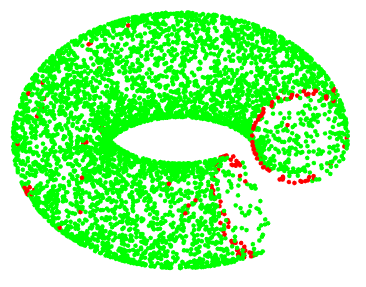
(h) SPINVER

Figure 4. The plot of $\mathcal{X}$ (green and red) and $\partial\mathcal{X}$ (red) for different algorithms in the vertical-cut torus example.

5.3. Tilted-cut torus

We uniformly randomly sample $\{\theta_{j}\}_{j=1}^{8000}$ and $\{\phi_{j}\}_{i=1}^{8000}$ from $[-\pi,\pi)$ respectively. Let $(u_{j},v_{j},w_{j})=(3+1.2\cos\theta_{j}\cos\phi_{j},3+1.2\cos\theta_{j}\sin\phi_{j},1.2\sin\theta_{j})$ be a point on a torus in $\mathbb{R}^{3}$. We rotate the points $\{(x_{j},y_{j},z_{j})\}_{j=1}^{8000}$ around the y-axis through the following map,

$$(u_{j},v_{j},w_{j})\rightarrow(u^{\prime}_{j},v^{\prime}_{j},w^{\prime}_{j})=(\cos(\frac{3\pi}{4})u_{j}-\sin(\frac{3\pi}{4})w_{j},v_{j},\sin(\frac{3\pi}{4})u_{j}+\cos(\frac{3\pi}{4})w_{j}).$$

$\mathcal{X}\subset\mathbb{R}^{3}$ consists of the points $\{(u^{\prime}_{j},v^{\prime}_{j},w^{\prime}_{j})\}$ with $w^{\prime}_{j}<2.8$. Thus, we generate $7596$ non-uniform samples $\mathcal{X}=\{z_{i}\}_{i=1}^{7596}$ on the tilted-cut torus. We apply BD-LLE in the $\epsilon$-radius ball scheme to $\mathcal{X}$ with $\epsilon=1.25$. We summarize the scale parameters used in other algorithms in Table 2, and $F1_{\max}$ for all the algorithms in Table 3. We plot $\mathcal{X}$ and the detected boundary points $\partial\mathcal{X}$ for each algorithm in Figure 5.

24

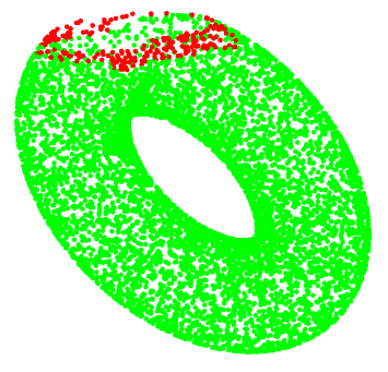
(a) BD-LLE

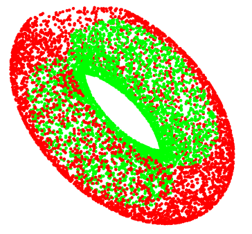
(b) $\alpha$-shape

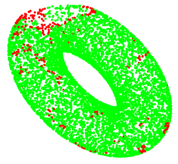
(c) BAND

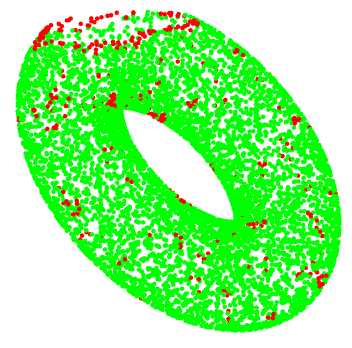
(d) BORDER

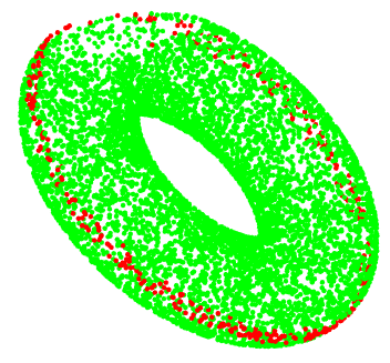
(e) BRIM

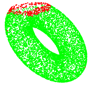
(f) Calder

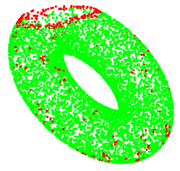
(g) LEVER

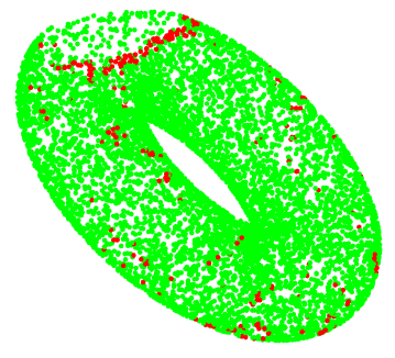
(h) SPINVER

Figure 5. The plot of $\mathcal{X}$ (green and red) and $\partial\mathcal{X}$ (red) for different algorithms in the tilted-cut torus example.

In the above results, $\alpha$-shape algorithm can successfully detects the boundary points when the dimension of $M$ equals the dimension of the ambient space, regardless of the distributions of the data. However, it fails to handle the scenario when the manifold $M$ has a lower dimension. BAND, BORDER, BRIM, LEVER, and SPINVER algorithms struggle to detect boundary points due to both the non-uniform distribution of the data and the extrinsic curvature of $\iota(M)$. In contrast, BD-LLE successfully identifies the boundary points in all examples and exhibits the best performance in vertical-cut torus and tilted-cut torus examples, regardless of the extrinsic geometry of the manifold and data distributions. For a more detailed discussion of algorithms other than BD-LLE, refer to Section D of the Supplementary Material.

6. Discussion

In this work, we delve into the challenge of identifying boundary points from samples on an embedded compact manifold with boundary. We introduce the BD-LLE algorithm, which utilizes barycentric coordinates within the framework of LLE. This algorithm can be implemented using either an $\epsilon$-radius ball scheme or a KNN scheme. Barycentric coordinates are closely related to the local covariance matrix. We conduct bias and variance analyses and explore the spectral properties of the local covariance matrix under both nearest neighbor search schemes to aid in parameter selection and analyze the BD-LLE algorithm. We highlight several directions for future research.

As discussed previously, the LLE can be considered as a kernel-based dimension reduction method with (2.11) representing an asymmetric kernel function adaptive to the data distribution and the geometry of the underlying manifold. The previous studies [26, 28] analyze the LLE within the $\epsilon$-radius ball scheme. A future direction involves applying our developed tools to analyze LLE within the KNN scheme. We expect establishing even more challenging results of the spectral convergence of the LLE in the KKN scheme on manifolds with or without boundary.

Another potential direction of research concerns the boundary points augmentation. Given that the boundary is a lower dimensional subset of the manifold, the limited number of boundary points may not suffice for accurately capturing the geometry of the boundary. Notably, the boundary comprises disjoint unions of closed manifolds without boundary. Hence, one strategy involves applying spectral clustering method to organize detected boundary points into groups corresponding to different connected components. Closed manifold reconstruction methods [12] can be further employed on each group to interpolate more points on the boundary.

Appendix A Proof of Theorem 4.2

A.1. Preliminary definitions

Under Assumptions 3.1 and 3.2, let $X$ be the random variable associated with the probability density function $P$ on $M$. Then, for any function $f$ on $M$ and any function $F$ on $\iota(M)$, we have

$$\mathbb{E}[f(X)]:=\int_{M}f(x)d\mathsf{P}=\int_{M}f(x)P(x)dV(x),$$

$$\mathbb{E}[F(\iota(X))f(X)]:=\int_{M}F(\iota(x))f(x)d\mathsf{P}=\int_{M}F(\iota(x))f(x)P(x)dV(x)\in\mathbb{R}^{p}.$$

Based on the above definitions, the expectation of the local covariance matrix at $\iota(x)$ is defined as

$$C_{x}:=\mathbb{E}[(\iota(X)-\iota(x))(\iota(X)-\iota(x))^{\top}\chi_{\big{(}B^{\mathbb{R}^{p}}_{\epsilon}(\iota(x))\cap\iota(M)\big{)}}(\iota(X))]\in\mathbb{R}^{p\times p}.$$

Suppose $\texttt{rank}(C_{x})=r\leq p$. Clearly $r$ depends on $x$, but we ignore $x$ for the simplicity. Denote the eigen-decomposition of $C_{x}$ as $C_{x}=U_{x}\Lambda_{x}U_{x}^{\top}$, where $U_{x}\in O(p)$ is composed of eigenvectors and $\Lambda_{x}$ is a diagonal matrix with the associated eigenvalues $\lambda_{1}\geq\lambda_{2}\geq\cdots\geq\lambda_{r}>\lambda_{r+1}=\cdots=\lambda_{p}=0$.

Through the eigenpairs of $C_{x}$, we can construct an augmented vector $\mathbf{T}(x)$ at $x\in M$.

Definition A.1.

The augmented vector at $x\in M$ is

$$\mathbf{T}(x)^{\top} =\mathbb{E}[(\iota(X)-\iota(x))\chi_{\big{(}B^{\mathbb{R}^{p}}_{\epsilon}(\iota(x))\cap\iota(M)\big{)}}(\iota(X))]^{\top}U_{x}I_{p,r}(\Lambda_{x}+\epsilon^{d+3}I_{p\times p})^{-1}U_{x}^{\top}\in\mathbb{R}^{p}\,,$$

which is a $\mathbb{R}^{p}$-valued vector field on $M$.

A.2. Lemmas for the variance analysis

Form (3.1), we have

$$B_{k}=\frac{\mathbf{T}^{\top}_{n,x_{k}}G_{n,k}\bm{1}_{N_{k}}}{{N_{k}}}=\frac{\frac{1}{n\epsilon^{d}}\mathbf{T}^{\top}_{n,x_{k}}G_{n,k}\bm{1}_{N_{k}}}{\frac{1}{n\epsilon^{d}}{N_{k}}}.\,$$

We will study the terms $\frac{1}{n\epsilon^{d}}{N_{k}}$ and $\frac{1}{n\epsilon^{d}}\mathbf{T}^{\top}_{n,x_{k}}G_{n,k}\bm{1}_{N_{k}}$ seperately in the next two lemmas. We first introduce the following definitions.

Definition A.2.

Denote $B^{\mathbb{R}^{p}}$ to be a closed ball in $\mathbb{R}^{p}$ without specifying the center. We define the following collections of balls intersecting $\iota(M)$,

(A.1) $$\mathcal{B}_{r}(\iota(M))=\left\{B^{\mathbb{R}^{p}}\cap\iota(M)\Big{|}\,B^{\mathbb{R}^{p}}\cap\iota(M)\not=\emptyset,\mbox{radius of }B^{\mathbb{R}^{p}}\leq r\right\}\,.$$

If $A\in\mathcal{B}_{r}(\iota(M))$, then $N(A)=|A\cap\mathcal{X}|$.

By Definition 4.3, for any $x\in M$, $N_{a}(x)=|B_{a}^{\mathbb{R}^{p}}(\iota(x))\cap\mathcal{X}|$. Now, we are ready to provide the variance analysis which relates $\frac{1}{n\epsilon^{d}}{N_{\epsilon}(x)}$ to $\frac{1}{\epsilon^{d}}\mathbb{E}[\chi_{\big{(}B^{\mathbb{R}^{p}}_{\epsilon}(\iota(x))\cap\iota(M)\big{)}}(\iota(X))]$ for any $x\in M$.

Lemma A.1.

1. Suppose $\sup_{A\in\mathcal{B}_{2r}(\iota(M))}\mathbb{E}[\chi_{A}(\iota(X))]\leq b\leq\frac{1}{4}$. For $n$ large enough, with probability greater than $1-n^{-2}$,

   $$\sup_{A\in\mathcal{B}_{r}(\iota(M))}|\frac{N(A)}{n}-\mathbb{E}[\chi_{A}(\iota(X))]|=O(\sqrt{\frac{b\log(n)}{n}}).$$

2. Suppose $\epsilon=\epsilon(n)$ so that $\frac{\sqrt{\log(n)}}{n^{1/2}\epsilon^{d/2+1}}\to 0$ and $\epsilon\to 0$ as $n\to\infty$. We have with probability greater than $1-n^{-2}$ that for all $x\in M$,

   $$\left|\frac{N_{\epsilon}(x)}{n\epsilon^{d}}-\frac{1}{\epsilon^{d}}\mathbb{E}[\chi_{\big{(}B^{\mathbb{R}^{p}}_{\epsilon}(\iota(x))\cap\iota(M)\big{)}}(\iota(X))]\right|=O\Big{(}\frac{\sqrt{\log(n)}}{n^{1/2}\epsilon^{d/2}}\Big{)}\,,$$

   where the constant in $O\Big{(}\frac{\sqrt{\log(n)}}{n^{1/2}\epsilon^{d/2}}\Big{)}$ depends on the $C^{0}$ norm of $P$ and the second fundamental form of $\iota(M)$.

The proof of (1) in the above lemma is a direct consequence of Lemma A.3 in [27]. As shown in Remark A.1 in [27], the proof of Lemma A.3 in [27] does not rely on the underlying manifold structure. Hence, it still holds when $M$ is a manifold with boundary. The proof of (2) in Lemma A.1 is a consequence of (1) and is the same as the proof of Corollary 2.2 in [27]. The manifold structure is involved in the estimation of $\sup_{A\in\mathcal{B}_{2\epsilon}(\iota(M))}\mathbb{E}[\chi_{A}(\iota(X))]$ which is of order $\epsilon^{d}$.

Note that $N_{k}=N_{\epsilon}(x_{k})-1$. When $\frac{\sqrt{\log(n)}}{n^{1/2}\epsilon^{d/2+1}}\to 0$ and $n$ is large enough, $\frac{1}{n\epsilon^{d}}<\frac{\sqrt{\log(n)}}{n^{1/2}\epsilon^{d/2}}$. Hence, the following lemma is a consequence of (2) in Lemma A.1.

Lemma A.2.

Suppose $\epsilon=\epsilon(n)$ so that $\frac{\sqrt{\log(n)}}{n^{1/2}\epsilon^{d/2+1}}\to 0$ and $\epsilon\to 0$ as $n\to\infty$. We have with probability greater than $1-n^{-2}$ that for $k=1,\cdots,n$,

$$\left|\frac{1}{n\epsilon^{d}}\sum_{j=1}^{N_{k}}1-\frac{1}{\epsilon^{d}}\mathbb{E}[\chi_{\big{(}B^{\mathbb{R}^{p}}_{\epsilon}(\iota(x_{k}))\cap\iota(M)\big{)}}(\iota(X))]\right|=O\Big{(}\frac{\sqrt{\log(n)}}{n^{1/2}\epsilon^{d/2}}\Big{)}\,,$$

where the constant in $O\Big{(}\frac{\sqrt{\log(n)}}{n^{1/2}\epsilon^{d/2}}\Big{)}$ depends on the $C^{0}$ norm of $P$ and the second fundamental form of $\iota(M)$.

In the next lemma, we show that $\frac{1}{\epsilon^{d}}\mathbf{T}(x_{k})^{\top}\mathbb{E}(\iota(X)-\iota(x_{k}))\chi_{\big{(}B^{\mathbb{R}^{p}}_{\epsilon}(\iota(x_{k}))\cap\iota(M)\big{)}}(\iota(X))$ is the limit of $\frac{1}{n\epsilon^{d}}\mathbf{T}^{\top}_{n,x_{k}}G_{n,k}\bm{1}_{N_{k}}$ as $n\to\infty$ and we control the size of fluctuation. The lemma can be found as (F.50) in [28].

Lemma A.3.

Suppose $\epsilon=\epsilon(n)$ so that $\frac{\sqrt{\log(n)}}{n^{1/2}\epsilon^{d/2+1}}\to 0$ and $\epsilon\to 0$ as $n\to\infty$. Suppose $c=n\epsilon^{d+3}$ in the construction of $\mathbf{T}^{\top}_{n,x_{k}}$ in (2.10). We have with probability greater than $1-n^{-2}$ that for all $k=1,\ldots,n$,

(A.2) $$\frac{1}{n\epsilon^{d}}\mathbf{T}^{\top}_{n,x_{k}}G_{n,k}\bm{1}_{N_{k}}=\frac{1}{\epsilon^{d}}\mathbf{T}(x_{k})^{\top}\mathbb{E}(\iota(X)-\iota(x_{k}))\chi_{\big{(}B^{\mathbb{R}^{p}}_{\epsilon}(\iota(x_{k}))\cap\iota(M)\big{)}}(\iota(X))+O\Big{(}\frac{\sqrt{\log(n)}}{n^{1/2}\epsilon^{d/2}}\Big{)},$$

where the constant in $O\Big{(}\frac{\sqrt{\log(n)}}{n^{1/2}\epsilon^{d/2}}\Big{)}$ depends on $P_{m}$, the $C^{1}$ norm of $P$ and the second fundamental form of $\iota(M)$ at $\iota(x_{k})$.

A.3. Lemmas for the bias analysis

Recall the notations introduced in Definition 4.1,

$$x_{\partial}:=\arg\min_{y\in\partial M}d_{g}(y,x),\quad\quad\tilde{\epsilon}(x)=d_{g}(x_{\partial},x).$$

In this subsection, we study the terms $\frac{1}{\epsilon^{d}}\mathbb{E}[\chi_{B_{\epsilon}^{\mathbb{R}^{p}}(\iota(x_{k}))}(\iota(X))]$ and $\mathbb{E}[(\iota(X)-\iota(x_{k}))\chi_{B_{\epsilon}^{\mathbb{R}^{p}}(\iota(x_{k}))}(\iota(X))]$. The following lemma is a combination of Corollary B.1 and Lemma B.3 in [28].

Lemma A.4.

Under Assumptions 3.1, 3.2, and 4.1, when $\epsilon>0$ is sufficiently small, the following expansions hold.

1. $\mathbb{E}[\chi_{\big{(}B^{\mathbb{R}^{p}}_{\epsilon}(\iota(x))\cap\iota(M)\big{)}}(\iota(X))]=P(x)\sigma_{0}(\tilde{\epsilon}(x),\epsilon)\epsilon^{d}+O(\epsilon^{d+1})$, where $\sigma_{0}$ is defined in Definition 4.2 and the constant in $O(\epsilon^{d+1})$ depends on the $C^{1}$ norm of $P$.

2. $\mathbb{E}[(\iota(X)-\iota(x))\chi_{\big{(}B^{\mathbb{R}^{p}}_{\epsilon}(\iota(x))\cap\iota(M)\big{)}}(\iota(X))]=P(x)\sigma_{1,d}(\tilde{\epsilon}(x),\epsilon)\epsilon^{d+1}e_{d}+O(\epsilon^{d+2})$. $\sigma_{1,d}$ is defined in Definition 4.2. $O(\epsilon^{d+2})$ represents a vector in $\mathbb{R}^{p}$ whose entries are of order $O(\epsilon^{d+2})$. The constants in $O(\epsilon^{d+2})$ depend on the $C^{1}$ norm of $P$ and the second fundamental form of $\iota(M)$.

If we combine (2) in Lemma A.1 and (1) in Lemma A.4, we have the following strong uniform consistency of kernel density estimation through $0-1$ kernel on a manifold with boundary.

Proposition A.1.

Suppose $\epsilon=\epsilon(n)$ so that $\frac{\sqrt{\log(n)}}{n^{1/2}\epsilon^{d/2+1}}\to 0$ and $\epsilon\to 0$ as $n\to\infty$. We have with probability greater than $1-n^{-2}$ that for all $x\in M$,

$$\left|\frac{N_{\epsilon}(x)}{n\epsilon^{d}\sigma_{0}(\tilde{\epsilon}(x),\epsilon)}-P(x)\right|=O(\epsilon)+O\Big{(}\frac{\sqrt{\log(n)}}{n^{1/2}\epsilon^{d/2}}\Big{)}\,,$$

where $\sigma_{0}$ is defined in Definition 4.2, the constant $O(\epsilon)$ depends on the $C^{1}$ norm of $P$ and the constant in $O\Big{(}\frac{\sqrt{\log(n)}}{n^{1/2}\epsilon^{d/2}}\Big{)}$ depends on the $C^{0}$ norm of $P$ and the second fundamental form of $\iota(M)$.

By using the function in Definition 4.2, the bias analysis of the augmented vector is summarized in the following lemma. The lemma can be found as Proposition 3.1(or a combination of Corollary B.1 and Lemma D.1) in [28].

Lemma A.5.

Suppose Assumptions 3.1, 3.2, and 4.1 hold. If $x\in M_{\epsilon}$, then

$$\mathbf{T}(x)=\, \frac{\sigma_{1,d}(\tilde{\epsilon}(x),\epsilon)}{\sigma_{2,d}(\tilde{\epsilon}(x),\epsilon)}\frac{1}{\epsilon}e_{d}+\frac{P(x)}{2}\Bigg{[}\Big{(}\sigma_{2}(\tilde{\epsilon}(x),\epsilon)-\frac{\sigma_{1,d}(\tilde{\epsilon}(x),\epsilon)}{\sigma_{2,d}(\tilde{\epsilon}(x),\epsilon)}\sigma_{3}(\tilde{\epsilon}(x),\epsilon)\Big{)}v_{1}(x)$$

$$\qquad\qquad+\Big{(}\sigma_{2,d}(\tilde{\epsilon}(x),\epsilon)-\frac{\sigma_{1,d}(\tilde{\epsilon}(x),\epsilon)}{\sigma_{2,d}(\tilde{\epsilon}(x),\epsilon)}\sigma_{3,d}(\tilde{\epsilon}(x),\epsilon)\Big{)}v_{2}(x)\Bigg{]}\frac{1}{\epsilon}+O(1).$$

We have $v_{1}(x),v_{2}(x)\in(\iota_{*}T_{x}M)^{\bot}$. $O(1)$ represents a vector in $\mathbb{R}^{p}$ whose entries are of order $O(1)$. The constants in $O(1)$ depend on $P_{m}$, the $C^{1}$ norm of $P$ and the second fundamental form of $\iota(M)$ at $\iota(x)$.

If $x\in M\setminus M_{\epsilon}$, then

$$\mathbf{T}(x)=\, \frac{P(x)}{2}\bigg{[}\frac{|S^{d-1}|}{d(d+2)}v_{3}(x)\bigg{]}\frac{1}{\epsilon}+O(1),$$

where $v_{3}(x)\in(\iota_{*}T_{x}M)^{\bot}$. $O(1)$ represents a vector in $\mathbb{R}^{p}$ whose entries are of order $O(1)$. The constants in $O(1)$ depend on $P_{m}$, the $C^{1}$ norm of $P$, and the second fundamental form of $\iota(M)$ at $\iota(x)$.

A.4. Combining the bias and the variance analyses to prove Theorem 4.2

For any $x_{k}$, since $e_{d}$ belongs to $\iota_{*}T_{x_{k}}M$, we have $e_{d}^{\top}v_{j}(x_{k})=0$ for $j=1,2,3$. Thus, by (2) in Lemma A.4 and Lemma A.5, when $x_{k}\in M_{\epsilon}$,

(A.3) $$\mathbf{T}(x_{k})^{\top}\mathbb{E}(\iota(X)-\iota(x_{k}))\chi_{\big{(}B^{\mathbb{R}^{p}}_{\epsilon}(\iota(x_{k}))\cap\iota(M)\big{)}}(\iota(X))=P(x_{k})\frac{(\sigma_{1,d}(\tilde{\epsilon}(x_{k}),\epsilon))^{2}}{\sigma_{2,d}(\tilde{\epsilon}(x_{k}),\epsilon)}\epsilon^{d}+O(\epsilon^{d+1}),$$

where the constant in $O(\epsilon^{d+1})$ depends on $P_{m}$, the $C^{1}$ norm of $P$ and the second fundamental form of $\iota(M)$ at $\iota(x_{k})$. When $x_{k}\in M\setminus M_{\epsilon}$,

(A.4) $$\mathbf{T}(x_{k})^{\top}\mathbb{E}(\iota(X)-\iota(x_{k}))\chi_{\big{(}B^{\mathbb{R}^{p}}_{\epsilon}(\iota(x_{k}))\cap\iota(M)\big{)}}(\iota(X))=O(\epsilon^{d+1}),$$

the constant in $O(\epsilon^{d+1})$ depends on $P_{m}$, the $C^{1}$ norm of $P$ and the second fundamental form of $\iota(M)$ at $\iota(x_{k})$.

Suppose $\epsilon=\epsilon(n)$ so that $\frac{\sqrt{\log(n)}}{n^{1/2}\epsilon^{d/2+1}}\to 0$ and $\epsilon\to 0$ as $n\to\infty$. By (A.3), (A.4), and Lemma A.3, with probability greater than $1-n^{-2}$ that for any $x_{k}\in M_{\epsilon}$,

$$\frac{1}{n\epsilon^{d}}\mathbf{T}^{\top}_{n,x_{k}}G_{n,k}\bm{1}_{N_{k}}= \frac{1}{\epsilon^{d}}\mathbf{T}(x_{k})^{\top}\mathbb{E}(\iota(X)-\iota(x_{k}))\chi_{\big{(}B^{\mathbb{R}^{p}}_{\epsilon}(\iota(x_{k}))\cap\iota(M)\big{)}}(\iota(X))+O\Big{(}\frac{\sqrt{\log(n)}}{n^{1/2}\epsilon^{d/2}}\Big{)}$$

$$= P(x_{k})\frac{(\sigma_{1,d}(\tilde{\epsilon}(x_{k}),\epsilon))^{2}}{\sigma_{2,d}(\tilde{\epsilon}(x_{k}),\epsilon)}+O(\epsilon)+O\Big{(}\frac{\sqrt{\log(n)}}{n^{1/2}\epsilon^{d/2}}\Big{)},$$

and any $x_{k}\in M\setminus M_{\epsilon}$,

$$\frac{1}{n\epsilon^{d}}\mathbf{T}^{\top}_{n,x_{k}}G_{n,k}\bm{1}_{N_{k}}=O(\epsilon)+O\Big{(}\frac{\sqrt{\log(n)}}{n^{1/2}\epsilon^{d/2}}\Big{)},$$

where the constants in $O(\epsilon)$ and $O\Big{(}\frac{\sqrt{\log(n)}}{n^{1/2}\epsilon^{d/2}}\Big{)}$ depend on $P_{m}$, the $C^{1}$ norm of $P$ and the second fundamental form of $\iota(M)$ at $\iota(x_{k})$. Note that when $x_{k}\in M\setminus M_{\epsilon}$ , we have $\tilde{\epsilon}(x_{k})\geq\epsilon$. By the definition of $\sigma_{1,d}(\tilde{\epsilon}(x_{k}),\epsilon)$, $\frac{(\sigma_{1,d}(\tilde{\epsilon}(x_{k}),\epsilon))^{2}}{\sigma_{2,d}(\tilde{\epsilon}(x_{k}),\epsilon)}=0$ when $\tilde{\epsilon}(x_{k})\geq\epsilon$. Thus, we can combine the above two cases and we conclude that with probability greater than $1-n^{-2}$ for any $x_{k}$,

(A.5) $$\frac{1}{n\epsilon^{d}}\mathbf{T}^{\top}_{n,x_{k}}G_{n,k}\bm{1}_{N_{k}}=P(x_{k})\frac{(\sigma_{1,d}(\tilde{\epsilon}(x_{k}),\epsilon))^{2}}{\sigma_{2,d}(\tilde{\epsilon}(x_{k}),\epsilon)}+O(\epsilon)+O\Big{(}\frac{\sqrt{\log(n)}}{n^{1/2}\epsilon^{d/2}}\Big{)}.$$

By Lemma A.2 and (1) in Lemma A.4, with probability greater than $1-n^{-2}$ for any $x_{k}$,

(A.6) $$\frac{1}{n\epsilon^{d}}{N_{k}}=P(x_{k})\sigma_{0}(\tilde{\epsilon}(x_{k}),\epsilon)+O(\epsilon)+O\Big{(}\frac{\sqrt{\log(n)}}{n^{1/2}\epsilon^{d/2}}\Big{)},$$

where the constants in $O(\epsilon)$ and $O\Big{(}\frac{\sqrt{\log(n)}}{n^{1/2}\epsilon^{d/2}}\Big{)}$ depend on the $C^{1}$ norm of $P$ and the second fundamental form of $\iota(M)$.

By (3.1), $B_{k}=\frac{\frac{1}{n\epsilon^{d}}\mathbf{T}^{\top}_{n,x_{k}}G_{n,k}(x_{k})\bm{1}_{N_{k}}}{\frac{1}{n\epsilon^{d}}{N_{k}}}$. By (A.5) and (A.6) and taking a union bound, with probability greater than $1-2n^{-2}$ for any $x_{k}$,

$$B_{k}=\frac{P(x_{k})\frac{(\sigma_{1,d}(\tilde{\epsilon}(x_{k}),\epsilon))^{2}}{\sigma_{2,d}(\tilde{\epsilon}(x_{k}),\epsilon)}+O(\epsilon)+O\Big{(}\frac{\sqrt{\log(n)}}{n^{1/2}\epsilon^{d/2}}\Big{)}}{P(x_{k})\sigma_{0}(\tilde{\epsilon}(x_{k}),\epsilon)+O(\epsilon)+O\Big{(}\frac{\sqrt{\log(n)}}{n^{1/2}\epsilon^{d/2}}\Big{)}}.$$

Note that $\sigma_{0}(\tilde{\epsilon}(x_{k}),\epsilon)$ is bounded from below and from above by constants. Hence,

(A.7) $$B_{k}=\frac{(\sigma_{1,d}(\tilde{\epsilon}(x_{k}),\epsilon))^{2}}{\sigma_{0}(\tilde{\epsilon}(x_{k}),\epsilon)\sigma_{2,d}(\tilde{\epsilon}(x_{k}),\epsilon)}+O(\epsilon)+O\Big{(}\frac{\sqrt{\log(n)}}{n^{1/2}\epsilon^{d/2}}\Big{)},$$

where the constants in $O(\epsilon)$ and $O\Big{(}\frac{\sqrt{\log(n)}}{n^{1/2}\epsilon^{d/2}}\Big{)}$ depend on $P_{m}$, the $C^{1}$ norm of $P$ and the second fundamental form of $\iota(M)$.

The properties (1), (2), (3), (4) and (5) follow directly from Proposition 4.1 and the definitions of $\tilde{\epsilon}(x)$, $\sigma_{0}(\tilde{\epsilon}(x),\epsilon)$, $\sigma_{1,d}(\tilde{\epsilon}(x),\epsilon)$, and $\sigma_{2,d}(\tilde{\epsilon}(x),\epsilon)$. (6) follows from (1), (3), and (4).

Appendix B Proofs of Proposition 4.2 and Proposition 4.3

B.1. Proof of Proposition 4.3

We first prove the following lemma about $V(t,r)$ and $U(t,s)$.

Lemma B.1.

1. When $\delta$ is small enough depending on $d$, $V(t,r(1-\delta))\leq V(t,r)(1-C\delta)$ and $V(t,r(1+\delta))\geq V(t,r)(1+C\delta)$, where $C>0$ is a constant depending on $d$.

2. For any $t$, we have $(\frac{d}{|S^{d-1}|})^{\frac{1}{d}}s^{\frac{1}{d}}\leq U(t,s)\leq(\frac{2d}{|S^{d-1}|})^{\frac{1}{d}}s^{\frac{1}{d}}$

Proof.

(1) We prove $V(t,r(1-\delta))\geq V(t,r)(1-C\delta)$, while $V(t,r(1+\delta))\leq V(t,r)(1+C\delta)$ can be proved similarly. Without loss of generality, suppose $t<r(1-\delta)<r$. The cases when $r(1-\delta)<t<r$ or $r(1-\delta)<r<t$ are straightforward. By the definition of $V(t,r)$,

$$V(t,r)-V(t,r(1-\delta))$$

$$= \frac{|S^{d-1}|}{2d}r^{d}(1-(1-\delta)^{d})+\frac{|S^{d-2}|}{d-1}\int_{0}^{t}\big{[}(r^{2}-x^{2})^{\frac{d-1}{2}}-(r^{2}(1-\delta)^{2}-x^{2})^{\frac{d-1}{2}}\big{]}dx$$

$$= \frac{|S^{d-1}|}{2d}r^{d}(1-(1-\delta)^{d})+\frac{|S^{d-2}|}{d-1}\int_{0}^{t}(r^{2}-x^{2})^{\frac{d-1}{2}}\big{[}1-(\frac{r^{2}(1-\delta)^{2}-x^{2}}{r^{2}-x^{2}})^{\frac{d-1}{2}}\big{]}dx$$

$$= \frac{|S^{d-1}|}{2d}r^{d}(1-(1-\delta)^{d})+\frac{|S^{d-2}|}{d-1}\int_{0}^{t}(r^{2}-x^{2})^{\frac{d-1}{2}}\big{[}1-(1-\frac{2\delta r^{2}-r^{2}\delta^{2}}{r^{2}-x^{2}})^{\frac{d-1}{2}}\big{]}dx$$

$$= \frac{|S^{d-1}|}{2d}r^{d}(1-(1-\delta)^{d})+\frac{|S^{d-2}|}{d-1}\int_{0}^{t}(r^{2}-x^{2})^{\frac{d-1}{2}}\big{[}1-(1-\frac{2\delta-\delta^{2}}{1-x^{2}/r^{2}})^{\frac{d-1}{2}}\big{]}dx$$

$$\geq \frac{|S^{d-1}|}{2d}r^{d}(1-(1-\delta)^{d})+\frac{|S^{d-2}|}{d-1}\int_{0}^{t}(r^{2}-x^{2})^{\frac{d-1}{2}}\big{[}1-(1-2\delta+\delta^{2})^{\frac{d-1}{2}}\big{]}dx$$

$$= \frac{|S^{d-1}|}{2d}r^{d}(1-(1-\delta)^{d})+\frac{|S^{d-2}|}{d-1}\int_{0}^{t}(r^{2}-x^{2})^{\frac{d-1}{2}}\big{[}1-(1-\delta)^{d-1}\big{]}dx$$

$$\geq \frac{d}{2}\delta\frac{|S^{d-1}|}{2d}r^{d}+\frac{d-1}{2}\frac{|S^{d-2}|}{d-1}\int_{0}^{t}(r^{2}-x^{2})^{\frac{d-1}{2}}dx\geq\frac{d-1}{2}\delta V(t,r).$$

Note that in the second last step we use the fact that $1-(1-\delta)^{d}\geq\frac{d}{2}\delta$ when $\delta$ is small enough depending on $d$.

(2) Fix any $s$, $r=U(t,s)$ is the radius of the region $\mathcal{R}_{t,r}$ with volume $s$ bounded between the ball of radius $r$ centered at the origin in $\mathbb{R}^{d}$ and the hyperplane $x_{d}=t$. The radius of the region achieves maximum when $t=0$, i.e. $s=\frac{|S^{d-1}|}{2d}r^{d}$. Hence $U(t,s)\leq(\frac{2d}{|S^{d-1}|})^{\frac{1}{d}}s^{\frac{1}{d}}$. The radius of the region achieves minimum when $t\geq(\frac{d}{|S^{d-1}|})^{\frac{1}{d}}s^{\frac{1}{d}}$, i.e. when $\mathcal{R}_{t,r}$ is the ball of volume of $s$ . Hence $U(t,s)\geq(\frac{d}{|S^{d-1}|})^{\frac{1}{d}}s^{\frac{1}{d}}$ ∎

Prove Proposition 4.3 by applying Lemma B.1

We estimate the probability of the events $\{R(x)\leq\tilde{R}(x)(1-\delta)\}$ and $\{R(x)\geq\tilde{R}(x)(1+\delta)\}$. Based on the definition of $R(x)$, the event of $\{R(x)\leq\tilde{R}(x)(1-\delta)\}$ is same as the event that $\{N_{\tilde{R}(x)(1-\delta)}(x)\geq K+1\}$. Thus, we have

(B.1) $$\Pr\big{\{}R(x)\leq\tilde{R}(x)(1-\delta)\big{\}}=\Pr\big{\{}\frac{1}{n}N_{\tilde{R}(x)(1-\delta)}(x)\geq\frac{K+1}{n}\big{\}}.$$

Similarly, we have

(B.2) $$\Pr\big{\{}R(x)\geq\tilde{R}(x)(1+\delta)\big{\}}=\Pr\big{\{}\frac{1}{n}N_{\tilde{R}(x)(1+\delta)}(x)\leq\frac{K+1}{n}\big{\}}.$$

We start to evaluate $\Pr\big{\{}\frac{1}{n}N_{\tilde{R}(x)(1-\delta)}(x)\geq\frac{K+1}{n}\big{\}}$. By (2) in Lemma B.1,

(B.3) $$\tilde{R}(x)=U(\tilde{\epsilon}(x),\frac{K+1}{P(x)n})\leq(\frac{2d}{|S^{d-1}|})^{\frac{1}{d}}(\frac{K+1}{P_{m}n})^{\frac{1}{d}}:=C_{1}(\frac{K+1}{n})^{\frac{1}{d}}.$$

Define $\tilde{R}^{*}:=C_{1}(\frac{K+1}{n})^{\frac{1}{d}}$. Recall the definitions of $B^{\mathbb{R}^{p}}_{r}$ and $\mathcal{B}_{r}(\iota(M))$ in Definition A.2. Observe that for any $r>0$, no matter where the center of $B^{\mathbb{R}^{p}}_{r}$ is, if $B^{\mathbb{R}^{p}}_{r}\cap\iota(M)\not=\emptyset$, then $B^{\mathbb{R}^{p}}_{r}\cap\iota(M)\subset B^{\mathbb{R}^{p}}_{2r}(\iota(x^{\prime}))\cap\iota(M)$ for $\iota(x^{\prime})\in B^{\mathbb{R}^{p}}_{r}\cap\iota(M)$. Hence, by (1) in Lemma A.4,

(B.4) $$\sup_{A\in\mathcal{B}_{4\tilde{R}^{*}}(\iota(M))}\mathbb{E}[\chi_{A}(\iota(X))]\leq\sup_{x^{\prime}\in M}\mathbb{E}[\chi_{\big{(}B^{\mathbb{R}^{p}}_{8\tilde{R}^{*}}(\iota(x^{\prime}))\cap\iota(M)\big{)}}(\iota(X))]\leq C_{2}(\frac{K+1}{n}),$$

where $C_{2}$ depends on $C^{0}$ norm of $P$ and $P_{m}$.

By (1) in Lemma A.1, Suppose $\frac{K}{n}\rightarrow 0$ as $n\rightarrow\infty$, then $C_{2}(\frac{K+1}{n})\leq\frac{1}{4}$. For $n$ large enough, with probability greater than $1-n^{-2}$, for all $x$,

(B.5) $$|\frac{1}{n}N_{\tilde{R}(x)(1-\delta)}(x)-\mathbb{E}[\chi_{\big{(}B^{\mathbb{R}^{p}}_{\tilde{R}(x)(1-\delta)}(\iota(x))\cap\iota(M)\big{)}}(\iota(X))]|$$

$$\leq \sup_{A\in\mathcal{B}_{2\tilde{R}^{*}}(\iota(M))}|\frac{N(A)}{n}-\mathbb{E}[\chi_{A}(\iota(X))]|\leq C_{3}\frac{\sqrt{(K+1)\log(n)}}{n},$$

where $C_{3}$ depends on $C^{0}$ norm of $P$ and $P_{m}$.

Next, we derive the condition on $\delta$ such that $\frac{1}{n}N_{\tilde{R}(x)(1-\delta)}(x)\geq\frac{K+1}{n}$ implies

(B.6) $$\frac{1}{n}N_{\tilde{R}(x)(1-\delta)}(x)-\mathbb{E}[\chi_{\big{(}B^{\mathbb{R}^{p}}_{\tilde{R}(x)(1-\delta)}(\iota(x))\cap\iota(M)\big{)}}(\iota(X))]\geq C_{3}\frac{\sqrt{(K+1)\log(n)}}{n}.$$

If we subtract both sides of $\frac{1}{n}N_{\tilde{R}(x)(1-\delta)}(x)\geq\frac{K+1}{n}$ by $\mathbb{E}[\chi_{\big{(}B^{\mathbb{R}^{p}}_{\tilde{R}(x)(1-\delta)}(\iota(x))\cap\iota(M)\big{)}}(\iota(X))]$, we have

(B.7) $$\frac{1}{n}N_{\tilde{R}(x)(1-\delta)}(x)-\mathbb{E}[\chi_{\big{(}B^{\mathbb{R}^{p}}_{\tilde{R}(x)(1-\delta)}(\iota(x))\cap\iota(M)\big{)}}(\iota(X))]$$

$$\geq \frac{K+1}{n}-\mathbb{E}[\chi_{\big{(}B^{\mathbb{R}^{p}}_{\tilde{R}(x)(1-\delta)}(\iota(x))\cap\iota(M)\big{)}}(\iota(X))]$$

$$\geq \frac{K+1}{n}-P(x)V(\tilde{\epsilon}(x),\tilde{R}(x)(1-\delta))-C_{4}\big{(}\tilde{R}(x)(1-\delta)\big{)}^{d+1}$$

$$\geq \frac{K+1}{n}-P(x)V(\tilde{\epsilon}(x),\tilde{R}(x))+C\delta P(x)V(\tilde{\epsilon}(x),\tilde{R}(x))-C_{4}\big{(}\tilde{R}(x)(1-\delta)\big{)}^{d+1}$$

$$= C\delta\frac{K+1}{n}-C_{4}\big{(}\tilde{R}(x)(1-\delta)\big{)}^{d+1}.$$

where $C_{4}>0$ depends on $C^{1}$ norm of $P$. Lemma A.4 is applied in the third last step, Lemma B.1 is applied in the second last step, and the definitions of the function $V$ and the term $\tilde{R}(x)$ are applied in the last step. If

(B.8) $$C\delta\frac{K+1}{n}-C_{4}\big{(}\tilde{R}(x)(1-\delta)\big{)}^{d+1}\geq C_{3}\frac{\sqrt{(K+1)\log(n)}}{n},$$

then we have (B.6). Hence,

$$\Pr\big{\{}\frac{1}{n}N_{\tilde{R}(x)(1-\delta)}(x)\geq\frac{K+1}{n}\big{\}}$$

$$\leq \Pr\Bigg{\{}\Big{(}\frac{1}{n}N_{\tilde{R}(x)(1-\delta)}(x)-\mathbb{E}[\chi_{\big{(}B^{\mathbb{R}^{p}}_{\tilde{R}(x)(1-\delta)}(\iota(x))\cap\iota(M)\big{)}}(\iota(X))]\Big{)}\geq C_{3}\frac{\sqrt{(K+1)\log(n)}}{n}\Bigg{\}}$$

$$\leq \Pr\Bigg{\{}\Big{|}\frac{1}{n}N_{\tilde{R}(x)(1-\delta)}(x)-\mathbb{E}[\chi_{\big{(}B^{\mathbb{R}^{p}}_{\tilde{R}(x)(1-\delta)}(\iota(x))\cap\iota(M)\big{)}}(\iota(X))]\Big{|}\geq C_{3}\frac{\sqrt{(K+1)\log(n)}}{n}\Bigg{\}}\leq n^{-2}.$$

In order to have (B.8), it suffices to require

(B.9) $$\frac{C}{2}\delta\frac{K+1}{n}\geq C_{4}(\tilde{R}^{*})^{d+1}\geq C_{4}\big{(}\tilde{R}(x)(1-\delta)\big{)}^{d+1},$$

and

(B.10) $$\frac{C}{2}\delta\frac{K+1}{n}\geq C_{3}\frac{\sqrt{(K+1)\log(n)}}{n}.$$

(B.9) is equivalent to $\delta\geq\frac{2C_{4}}{C}C_{1}^{d+1}(\frac{K+1}{n})^{\frac{1}{d}}$ and (B.10) is equivalent to $\delta\geq\frac{2C_{3}}{C}\sqrt{\frac{\log(n)}{K+1}}$. If $\frac{\log(n)}{K+1}(\frac{n}{K+1})^{2/d}\to 0$ as $n\to\infty$, then we have $\frac{2C_{4}}{C}C_{1}^{d+1}(\frac{K+1}{n})^{\frac{1}{d}}\geq\frac{2C_{3}}{C}\sqrt{\frac{\log(n)}{K+1}}$. Hence, it suffices to require $\delta\geq\frac{2C_{4}}{C}C_{1}^{d+1}(\frac{K+1}{n})^{\frac{1}{d}}$ which is guaranteed by $\delta\geq\frac{4C_{4}}{C}C_{1}^{d+1}(\frac{K}{n})^{\frac{1}{d}}$. Therefore, we choose $\delta=\frac{4C_{4}}{C}C_{1}^{d+1}(\frac{K}{n})^{\frac{1}{d}}$. At last, note that $\frac{\log(n)}{K+1}(\frac{n}{K+1})^{2/d}\to 0$ is equivalent to $\frac{\log(n)}{K}(\frac{n}{K})^{2/d}\to 0$.

Hence, we show that if $\frac{K}{n}\rightarrow 0$ and $\frac{\log(n)}{K}(\frac{n}{K})^{2/d}\to 0$ as $n\to\infty$, than with probability less than $n^{-2}$, for all $x$, $R(x)\leq\tilde{R}(x)(1-\delta)$, where $\delta=\frac{4C_{4}}{C}C_{1}^{d+1}(\frac{K}{n})^{\frac{1}{d}}$.

By (B.3), if $\delta$ is small, $\tilde{R}(x)(1+\delta)\leq 2\tilde{R}^{*}$. By (1) in Lemma A.1, suppose $\frac{K}{n}\rightarrow 0$ as $n\rightarrow\infty$, then $C_{2}(\frac{K+1}{n})\leq\frac{1}{4}$. Hence, for $n$ large enough, with probability greater than $1-n^{-2}$, for all $x$,

(B.11) $$|\frac{1}{n}N_{\tilde{R}(x)(1+\delta)}(x)-\mathbb{E}[\chi_{\big{(}B^{\mathbb{R}^{p}}_{\tilde{R}(x)(1+\delta)}(\iota(x))\cap\iota(M)\big{)}}(\iota(X))]|$$

$$\leq \sup_{A\in\mathcal{B}_{2\tilde{R}^{*}}(\iota(M))}|\frac{N(A)}{n}-\mathbb{E}[\chi_{A}(\iota(X))]|\leq C_{3}\frac{\sqrt{(K+1)\log(n)}}{n},$$

where $C_{3}$ depends on $C^{0}$ norm of $P$ and $P_{m}$.

We derive the condition on $\delta$ such that $\frac{1}{n}N_{\tilde{R}(x)(1+\delta)}(x)\leq\frac{K+1}{n}$ implies

(B.12) $$\frac{1}{n}N_{\tilde{R}(x)(1+\delta)}(x)-\mathbb{E}[\chi_{\big{(}B^{\mathbb{R}^{p}}_{\tilde{R}(x)(1+\delta)}(\iota(x))\cap\iota(M)\big{)}}(\iota(X))]\leq-C_{3}\frac{\sqrt{(K+1)\log(n)}}{n}.$$

If we subtract both sides of $\frac{1}{n}N_{\tilde{R}(x)(1+\delta)}(x)\leq\frac{K+1}{n}$ by $\mathbb{E}[\chi_{\big{(}B^{\mathbb{R}^{p}}_{\tilde{R}(x)(1+\delta)}(\iota(x))\cap\iota(M)\big{)}}(\iota(X))]$, we have

(B.13) $$\frac{1}{n}N_{\tilde{R}(x)(1+\delta)}(x)-\mathbb{E}[\chi_{\big{(}B^{\mathbb{R}^{p}}_{\tilde{R}(x)(1+\delta)}(\iota(x))\cap\iota(M)\big{)}}(\iota(X))]$$

$$\leq \frac{K+1}{n}-\mathbb{E}[\chi_{\big{(}B^{\mathbb{R}^{p}}_{\tilde{R}(x)(1+\delta)}(\iota(x))\cap\iota(M)\big{)}}(\iota(X))]$$

$$\leq \frac{K+1}{n}-P(x)V(\tilde{\epsilon}(x),\tilde{R}(x)(1+\delta))+C_{4}\big{(}\tilde{R}(x)(1+\delta)\big{)}^{d+1}$$

$$\leq \frac{K+1}{n}-P(x)V(\tilde{\epsilon}(x),\tilde{R}(x))-C\delta P(x)V(\tilde{\epsilon}(x),\tilde{R}(x))+C_{4}\big{(}\tilde{R}(x)(1+\delta)\big{)}^{d+1}$$

$$= C_{4}\big{(}\tilde{R}(x)(1+\delta)\big{)}^{d+1}-C\delta\frac{K+1}{n}.$$

where $C_{4}>0$ depends on $C^{1}$ norm of $P$. Lemma A.4 is applied in the third last step, Lemma B.1 is applied in the second last step, and the definitions of the function $V$ and the term $\tilde{R}(x)$ are applied in the last step. If

(B.14) $$C_{4}\big{(}\tilde{R}(x)(1+\delta)\big{)}^{d+1}-C\delta\frac{K+1}{n}\leq-C_{3}\frac{\sqrt{(K+1)\log(n)}}{n},$$

then we have (B.12). Hence,

$$\Pr\big{\{}\frac{1}{n}N_{\tilde{R}(x)(1+\delta)}(x)\leq\frac{K+1}{n}\big{\}}$$

$$\leq \Pr\Bigg{\{}\Big{(}\frac{1}{n}N_{\tilde{R}(x)(1+\delta)}(x)-\mathbb{E}[\chi_{\big{(}B^{\mathbb{R}^{p}}_{\tilde{R}(x)(1+\delta)}(\iota(x))\cap\iota(M)\big{)}}(\iota(X))]\Big{)}\leq-C_{3}\frac{\sqrt{(K+1)\log(n)}}{n}\Bigg{\}}$$

$$\leq \Pr\Bigg{\{}\Big{|}\frac{1}{n}N_{\tilde{R}(x)(1+\delta)}(x)-\mathbb{E}[\chi_{\big{(}B^{\mathbb{R}^{p}}_{\tilde{R}(x)(1+\delta)}(\iota(x))\cap\iota(M)\big{)}}(\iota(X))]\Big{|}\geq C_{3}\frac{\sqrt{(K+1)\log(n)}}{n}\Bigg{\}}\leq n^{-2}.$$

In order to have (B.14), it suffices to require

(B.15) $$\frac{C}{2}\delta\frac{K+1}{n}\geq C_{4}(2\tilde{R}^{*})^{d+1}\geq C_{4}\big{(}\tilde{R}(x)(1+\delta)\big{)}^{d+1},$$

and

(B.16) $$\frac{C}{2}\delta\frac{K+1}{n}\geq C_{3}\frac{\sqrt{(K+1)\log(n)}}{n}.$$

Note that (B.15) is equivalent to $\delta\geq\frac{2^{d+2}C_{4}}{C}C_{1}^{d+1}(\frac{K+1}{n})^{\frac{1}{d}}$ and (B.16) is equivalent to $\delta\geq\frac{2C_{3}}{C}\sqrt{\frac{\log(n)}{K+1}}$. If $\frac{\log(n)}{K+1}(\frac{n}{K+1})^{2/d}\to 0$ as $n\to\infty$, then we have $\frac{2^{d+2}C_{4}}{C}C_{1}^{d+1}(\frac{K+1}{n})^{\frac{1}{d}}\geq\frac{2C_{3}}{C}\sqrt{\frac{\log(n)}{K+1}}$. Hence, it suffices to require $\delta\geq\frac{2^{d+2}C_{4}}{C}C_{1}^{d+1}(\frac{K+1}{n})^{\frac{1}{d}}$ which is guaranteed by $\delta\geq\frac{2^{d+3}C_{4}}{C}C_{1}^{d+1}(\frac{K}{n})^{\frac{1}{d}}$. Therefore, we choose $\delta=\frac{2^{d+3}C_{4}}{C}C_{1}^{d+1}(\frac{K}{n})^{\frac{1}{d}}$. At last, note that $\frac{\log(n)}{K+1}(\frac{n}{K+1})^{2/d}\to 0$ is equivalent to $\frac{\log(n)}{K}(\frac{n}{K})^{2/d}\to 0$.

Hence, we show that if $\frac{K}{n}\rightarrow 0$ and $\frac{\log(n)}{K}(\frac{n}{K})^{2/d}\to 0$ as $n\to\infty$, than with probability less than $n^{-2}$, for all $x$, $R(x)\geq\tilde{R}(x)(1+\delta)$, where $\delta=\frac{2^{d+3}C_{4}}{C}C_{1}^{d+1}(\frac{K}{n})^{\frac{1}{d}}$.

In conclusion if $\frac{K}{n}\rightarrow 0$ and $\frac{\log(n)}{K}(\frac{n}{K})^{2/d}\to 0$ as $n\to\infty$, than with probability greater than $1-2n^{-2}$, for all $x$, $R(x)=\tilde{R}(x)(1+O((\frac{K}{n})^{\frac{1}{d}}))$, where the constant in $O((\frac{K}{n})^{\frac{1}{d}})$ depends on $d$, $C^{1}$ norm of $P$, and $P_{m}$

When $n$ is large enough, we have $\frac{1}{2}\tilde{R}(x)\leq R(x)\leq\frac{3}{2}\tilde{R}(x)$. Hence, by (2) in Lemma B.1 and the definition of $\tilde{R}(x)$,

$$\frac{1}{2}(\frac{d}{|S^{d-1}|})^{\frac{1}{d}}(\frac{K}{P_{M}n})^{\frac{1}{d}}\leq\frac{1}{2}(\frac{d(K+1)}{|S^{d-1}|P_{M}n})^{\frac{1}{d}}\leq R(x)\leq\frac{3}{2}(\frac{2d(K+1)}{|S^{d-1}|P_{m}n})^{\frac{1}{d}}\leq 3(\frac{2d}{|S^{d-1}|})^{\frac{1}{d}}(\frac{K}{P_{m}n})^{\frac{1}{d}}.$$

Hence,

$$\frac{1}{2}(\frac{d}{|S^{d-1}|})^{\frac{1}{d}}(\frac{K}{P_{M}n})^{\frac{1}{d}}\leq R^{*}\leq 3(\frac{2d}{|S^{d-1}|})^{\frac{1}{d}}(\frac{K}{P_{m}n})^{\frac{1}{d}}.$$

B.2. Proof Proposition 4.2

(1) Consider $x,x^{\prime}\in M$. Assume $R(x^{\prime})\geq R(x)$. Observe that $B_{R(x)}(x)\subset B_{R(x)+\|\iota(x)-\iota(x^{\prime})\|_{\mathbb{R}^{p}}}(x^{\prime})$. Hence, $B_{R(x)+\|\iota(x)-\iota(x^{\prime})\|_{\mathbb{R}^{p}}}(x^{\prime})$ contains at least $K+1$ points. We have $R(x^{\prime})\leq R(x)+\|\iota(x)-\iota(x^{\prime})\|_{\mathbb{R}^{p}}$ , i.e. $R(x^{\prime})-R(x)\leq\|\iota(x)-\iota(x^{\prime})\|_{\mathbb{R}^{p}}$. Similarly, when $R(x^{\prime})\leq R(x)$, we have $R(x)-R(x^{\prime})\leq\|\iota(x)-\iota(x^{\prime})\|_{\mathbb{R}^{p}}$. Hence, $|R(x^{\prime})-R(x)|\leq\|\iota(x)-\iota(x^{\prime})\|_{\mathbb{R}^{p}}$. When $d_{g}(x,x^{\prime})\to 0$, then $\|\iota(x)-\iota(x^{\prime})\|_{\mathbb{R}^{p}}\to 0$ and $|R(x^{\prime})-R(x)|\to 0$.

(2) From the proof of (1), $|R(\gamma_{x}(t_{1}))-R(\gamma_{x}(t_{2}))|\leq\|\iota(\gamma_{x}(t_{1}))-\iota(\gamma_{x}(t_{2}))\|_{\mathbb{R}^{p}}$. Since $\gamma_{x}(t)$ is unit speed and mimizing on $[0,t_{2}]$, we have

(B.17) $$|R(\gamma_{x}(t_{1}))-R(\gamma_{x}(t_{2}))|\leq\|\iota(\gamma_{x}(t_{1}))-\iota(\gamma_{x}(t_{2}))\|_{\mathbb{R}^{p}}\leq t_{2}-t_{1}.$$

Observe that

$$\frac{t_{2}}{R(\gamma_{x}(t_{2}))}-\frac{t_{1}}{R(\gamma_{x}(t_{1}))}=\frac{R(\gamma_{x}(t_{1}))-t_{1}\frac{R(\gamma_{x}(t_{2}))-R(\gamma_{x}(t_{1}))}{t_{2}-t_{1}}}{R(\gamma_{x}(t_{1}))R(\gamma_{x}(t_{2}))/(t_{2}-t_{1}).}$$

If $R(\gamma_{x}(t_{2}))\leq R(\gamma_{x}(t_{1}))$, then $\frac{t_{2}}{R(\gamma_{x}(t_{2}))}>\frac{t_{1}}{R(\gamma_{x}(t_{1}))}$. If $R(\gamma_{x}(t_{2}))>R(\gamma_{x}(t_{1}))$, we have $\frac{R(\gamma_{x}(t_{2}))-R(\gamma_{x}(t_{1}))}{t_{2}-t_{1}}<1$. Hence, if $t_{1}<R(\gamma_{x}(t_{1}))$, then $\frac{t_{1}}{R(\gamma_{x}(t_{1}))}<\frac{t_{2}}{R(\gamma_{x}(t_{2}))}$. The conclusion follows.

Appendix C Proofs of Theorem 4.3 and Theorem 4.4

C.1. Proof of Theorem 4.3

First, we relate $C_{n,k}$ constructed through the KNN scheme to $C_{n,k}$ constructed through the $\epsilon$ radius ball scheme through $R(x)$ defined in Definition 4.3. Observe that for each $x_{k}$, $C_{n,k}$ constructed through the KNN scheme is equal to the $C_{n,k}$ constructed through the $R(x_{k})$-radius ball scheme. By Theorem 4.1, if for any $k$, $R(x_{k})\to 0$ and $\frac{\sqrt{\log(n)}}{n^{1/2}R(x_{k})^{d/2+1}}\to 0$ and as $n\to\infty$, then with probability greater than $1-2n^{-2}$, for all $k$,

(C.1) $$\frac{1}{n}C_{n,k}= P(x_{k}){\begin{bmatrix}M^{(0)}(x_{k},R(x_{k}))&0\\ 0&0\end{bmatrix}}R(x_{k})^{d+2}+\begin{bmatrix}M^{(11)}(x_{k},R(x_{k}))&M^{(12)}(x_{k},R(x_{k}))\\ M^{(21)}(x_{k},R(x_{k}))&0\end{bmatrix}R(x_{k})^{d+3}$$

$$+O(R(x_{k})^{d+4})+O\Big{(}\frac{\sqrt{\log(n)}}{n^{1/2}}R(x_{k})^{d/2+2}\Big{)}.$$

When $\tilde{\epsilon}(x_{k})\geq R^{*}$,

(C.2) $$\frac{1}{n}C_{n,k}= P(x_{k}){\begin{bmatrix}M^{(0)}(x_{k},R(x_{k}))&0\\ 0&0\end{bmatrix}}R(x_{k})^{d+2}+O(R(x_{k})^{d+4})+O\Big{(}\frac{\sqrt{\log(n)}}{n^{1/2}}R(x_{k})^{d/2+2}\Big{)}.$$

Second, we bound $R(x)$ by $\frac{K}{n}$. Using the same argument as in (C.3), by Proposition 4.3, suppose we have $\frac{K}{n}\rightarrow 0$ and $\frac{\log(n)}{K}(\frac{n}{K})^{2/d}\to 0$ as $n\to\infty$. , for all $x$, with probability greater than $1-2n^{-2}$,

$$\frac{1}{2}(\frac{d}{|S^{d-1}|})^{\frac{1}{d}}(\frac{K}{P_{M}n})^{\frac{1}{d}}\leq R(x)\leq 3(\frac{2d}{|S^{d-1}|})^{\frac{1}{d}}(\frac{K}{P_{m}n})^{\frac{1}{d}}.$$

Hence, $\frac{K}{n}\rightarrow 0$ is equivalent to $R(x_{k})\to 0$ and $\frac{\log(n)}{K}(\frac{n}{K})^{2/d}\to 0$ is equivalent to $\frac{\sqrt{\log(n)}}{n^{1/2}{R(x_{k})^{d/2+1}}}\to 0$. If we substitute the above bounds of $R(x)$ into (C.1) and (C.2), then with probability greater than $1-4n^{-2}$, we have

$$\frac{1}{n}C_{n,k}= P(x_{k}){\begin{bmatrix}M^{(0)}(x_{k},R(x_{k}))&0\\ 0&0\end{bmatrix}}R(x_{k})^{d+2}+\begin{bmatrix}\tilde{M}^{(11)}(x_{k},\frac{K}{n})&\tilde{M}^{(12)}(x_{k},\frac{K}{n})\\ \tilde{M}^{(21)}(x_{k},\frac{K}{n})&0\end{bmatrix}$$

$$+O((\frac{K}{n})^{\frac{d+4}{d}})+O\Big{(}\frac{\sqrt{K\log(n)}}{n}(\frac{K}{n})^{\frac{2}{d}}\Big{)}.$$

The magnitudes of the entries in $\tilde{M}^{(11)}(x_{k},\frac{K}{n})$ , $\tilde{M}^{(12)}(x_{k},\frac{K}{n})$, and $\tilde{M}^{(21)}(x_{k},\frac{K}{n})$ are bounded by $\tilde{C}(\frac{K}{n})^{\frac{d+3}{d}}$, where $\tilde{C}$ is constant depending on $d$, $P_{m}$, the $C^{1}$ norm of $P$, the second fundamental form of $\iota(M)$ in $\mathbb{R}^{p}$ at $\iota(x_{k})$, and the second fundamental form of $\partial M$ in $M$ at $x_{\partial,k}$.

When $\tilde{\epsilon}(x_{k})\geq R^{*}$,

$$\frac{1}{n}C_{n,k}= P(x_{k}){\begin{bmatrix}M^{(0)}(x_{k},R(x_{k}))&0\\ 0&0\end{bmatrix}}R(x_{k})^{d+2}+O((\frac{K}{n})^{\frac{d+4}{d}})+O\Big{(}\frac{\sqrt{K\log(n)}}{n}(\frac{K}{n})^{\frac{2}{d}}\Big{)}.$$

At last, we discuss the entries in $\tilde{M}^{(0)}(x)=P(x)M^{(0)}(x,R(x))R(x)^{d+2}$ for $x\in M$. $\tilde{M}^{(0)}(x)$ is a diagonal matrix. By Theorem 4.1 and Proposition 4.3, the $i$th diagonal entry of $\tilde{M}^{(0)}(x)$ is

$$P(x)\sigma_{2}(\tilde{\epsilon}(x),R(x))R(x)^{d+2}=P(x)\sigma_{2}(\tilde{\epsilon}(x),R(x))(\tilde{R}(x)(1+O((\frac{K}{n})^{\frac{1}{d}})))^{d+2},$$

for $i=1,\cdots,d-1$. And the $d$th diagonal entry is

$$P(x)\sigma_{2,d}(\tilde{\epsilon}(x),R(x))R(x)^{d+2}=P(x)\sigma_{2,d}(\tilde{\epsilon}(x),R(x))(\tilde{R}(x)(1+O((\frac{K}{n})^{\frac{1}{d}})))^{d+2}.$$

By (B.3), we can derive the following equalities,

$$P(x)\sigma_{2}(\tilde{\epsilon}(x),R(x))R(x)^{d+2}=P(x)\sigma_{2}(\tilde{\epsilon}(x),R(x))\tilde{R}(x)^{d+2}+O((\frac{K}{n})^{\frac{d+3}{d}}).$$

$$P(x)\sigma_{2,d}(\tilde{\epsilon}(x),R(x))R(x)^{d+2}=P(x)\sigma_{2,d}(\tilde{\epsilon}(x),R(x))\tilde{R}(x)^{d+2}+O((\frac{K}{n})^{\frac{d+3}{d}}).$$

Define $\mu_{1}(x)=P(x)\sigma_{2}(\tilde{\epsilon}(x),R(x))\tilde{R}(x)^{d+2}$ and $\mu_{2}(x)=P(x)\sigma_{2,d}(\tilde{\epsilon}(x),R(x))\tilde{R}(x)^{d+2}$.

Both $\mu_{1}(x)$ and $\mu_{2}(x)$ are continuous functions. We focus on $\mu_{1}(x)$, while $\mu_{2}(x)$ can be discussed similarly. Note that $\frac{|S^{d-1}|}{2d(d+2)}\leq\sigma_{2}(\tilde{\epsilon}(x),R(x))\leq\frac{|S^{d-1}|}{d(d+2)}$. By (2) in Lemma B.1 and the definition of $\tilde{R}(x)$, $(\frac{d}{|S^{d-1}|})^{\frac{d+2}{d}}(\frac{K+1}{P(x)n})^{\frac{d+2}{d}}\leq\tilde{R}(x)^{d+2}\leq(\frac{2d}{|S^{d-1}|})^{\frac{d+2}{d}}(\frac{K+1}{P(x)n})^{\frac{d+2}{d}}$. Hence,

$$\frac{1}{2(d+2)}(\frac{d}{|S^{d-1}|P_{M}})^{\frac{2}{d}}(\frac{K+1}{n})^{\frac{d+2}{d}}\leq\mu_{1}(x)\leq\frac{2}{d+2}(\frac{2d}{|S^{d-1}|P_{m}})^{\frac{2}{d}}(\frac{K+1}{n})^{\frac{d+2}{d}}.$$

When $x\in\partial M$, $\sigma_{2}(\tilde{\epsilon}(x),R(x))=\frac{|S^{d-1}|}{2d(d+2)}$ and $\tilde{R}(x)^{d+2}=(\frac{2d}{|S^{d-1}|})^{\frac{d+2}{d}}(\frac{K+1}{P(x)n})^{\frac{d+2}{d}}$. Therefore,

$$\mu_{1}(x)=\frac{1}{(d+2)}(\frac{2d}{|S^{d-1}|P(x)})^{\frac{2}{d}}(\frac{K+1}{n})^{\frac{d+2}{d}}.$$

The same results hold for $\mu_{2}(x)$.

When $\tilde{\epsilon}(x_{k})\geq R^{*}$,

$$\sigma_{2}(\tilde{\epsilon}(x_{k}),R(x_{k}))=\sigma_{2,d}(\tilde{\epsilon}(x_{k}),R(x_{k}))=\frac{|S^{d-1}|}{d(d+2)}.$$

Moreover, by (2) in Lemma B.1, $\tilde{R}(x_{k})=(\frac{d}{|S^{d-1}|})^{\frac{1}{d}}(\frac{K+1}{P(x_{k})n})^{\frac{1}{d}}$. Therefore,

$$\mu_{1}(x_{k})=\mu_{2}(x_{k})=\frac{1}{(d+2)}(\frac{d}{|S^{d-1}|P(x_{k})})^{\frac{2}{d}}(\frac{K+1}{n})^{\frac{d+2}{d}}.$$

C.2. Proof of Theorem 4.4

By Proposition 4.3, suppose $\frac{K}{n}\rightarrow 0$ and $\frac{\log(n)}{K}(\frac{n}{K})^{2/d}\to 0$ as $n\to\infty$. Then, for all $x$, with probability greater than $1-2n^{-2}$, we have $\frac{1}{2}\tilde{R}(x)\leq R(x)\leq\frac{3}{2}\tilde{R}(x)$. Hence, by (2) in Lemma B.1 and the definition of $\tilde{R}(x)$,

(C.3) $$\frac{1}{2}(\frac{d}{|S^{d-1}|})^{\frac{1}{d}}(\frac{K}{P_{M}n})^{\frac{1}{d}}\leq R(x)\leq 3(\frac{2d}{|S^{d-1}|})^{\frac{1}{d}}(\frac{K}{P_{m}n})^{\frac{1}{d}}.$$

Observe that for each $x_{k}$, $B_{k}$ constructed through the KNN scheme is equal to the $B_{k}$ constructed through the $R(x_{k})$-radius ball scheme. Based on the proof of Lemma A.3 and A.5 in [28], the conclusion of the lemmas still hold whenever we choose $\tilde{C}_{1}n\epsilon^{d+3}\leq c\leq\tilde{C}_{2}n\epsilon^{d+3}$, where $\tilde{C}_{1}$ and $\tilde{C}_{2}$ are constants independent of $n$ and $\epsilon$. Suppose we choose $\tilde{C}_{1}nR(x_{k})^{d+3}\leq c\leq\tilde{C}_{2}nR(x_{k})^{d+3}$ where $\tilde{C}_{1}$ and $\tilde{C}_{2}$ are constants independent of $n$ and $K$. By (A.7), if for any $k$, $R(x_{k})\to 0$ and $\frac{\sqrt{\log(n)}}{n^{1/2}R(x_{k})^{d/2+1}}\to 0$ and as $n\to\infty$, then with probability greater than $1-2n^{-2}$, for all $k$,

(C.4) $$B_{k}=\frac{(\sigma_{1,d}(\tilde{\epsilon}(x_{k}),R(x_{k})))^{2}}{\sigma_{0}(\tilde{\epsilon}(x_{k}),R(x_{k}))\sigma_{2,d}(\tilde{\epsilon}(x_{k}),R(x_{k}))}+O(R(x_{k}))+O\Big{(}\frac{\sqrt{\log(n)}}{n^{1/2}R(x_{k})^{d/2}}\Big{)}.$$

where $\tilde{\epsilon}(x_{k})$ is the distance from $x_{k}\in M$ to $\partial M$ as defined in (4.1). The constants in $O(R(x_{k}))$ and $O\Big{(}\frac{\sqrt{\log(n)}}{n^{1/2}R(x_{k})^{d/2}}\Big{)}$ depend on $P_{m}$, the $C^{1}$ norm of $P$ and the second fundamental form of $\iota(M)$. Moreover, if $\tilde{\epsilon}(x)$ is the distance from $x\in M$ to $\partial M$, then we define

$$\tilde{B}(x)=\frac{(\sigma_{1,d}(\tilde{\epsilon}(x),R(x)))^{2}}{\sigma_{0}(\tilde{\epsilon}(x),R(x))\sigma_{2,d}(\tilde{\epsilon}(x),R(x))}.$$

By (C.3), $\frac{K}{n}\rightarrow 0$ is equivalent to $R(x_{k})\to 0$ and $\frac{\log(n)}{K}(\frac{n}{K})^{2/d}\to 0$ is equivalent to $\frac{\sqrt{\log(n)}}{n^{1/2}{R(x_{k})^{d/2+1}}}\to 0$. Moreover, if $c=n(\frac{K}{n})^{\frac{d+3}{d}}$ , then

$$(\frac{2}{3})^{d+3}(\frac{|S^{d-1}|}{2d})^{\frac{d+3}{d}}P_{m}^{\frac{d+3}{d}}nR(x_{k})^{d+3}\leq c\leq 2^{d+3}(\frac{|S^{d-1}|}{d})^{\frac{d+3}{d}}P_{M}^{\frac{d+3}{d}}nR(x_{k})^{d+3}.$$

By taking the union bound for the probability, with probability greater than $1-4n^{-2}$, for all $k$, we have (C.3) for all $x_{k}$ and (C.4). If we substitute (C.3) into (C.4),

$$B_{k}=\frac{(\sigma_{1,d}(\tilde{\epsilon}(x_{k}),R(x_{k})))^{2}}{\sigma_{0}(\tilde{\epsilon}(x_{k}),R(x_{k}))\sigma_{2,d}(\tilde{\epsilon}(x_{k}),R(x_{k}))}+O((\frac{K}{n})^{\frac{1}{d}})+O\Big{(}\sqrt{\frac{\log(n)}{K}}\Big{)}.$$

The constants in $O(\frac{K}{n})^{\frac{1}{d}}$ and $O\Big{(}\sqrt{\frac{\log(n)}{K}}\Big{)}$ depend on $P_{m}$, the $C^{1}$ norm of $P$ and the second fundamental form of $\iota(M)$.

Next, we discuss the properties of $\tilde{B}(x)$. By Proposition 4.2 and the definitions of $\sigma_{0}$, $\sigma_{1,d}$, and $\sigma_{2,d}$, $\tilde{B}(x)$ is a continuous function on $M$. When $x\in\partial M$, $\tilde{\epsilon}(x)=0$ and we have $\tilde{B}(x)=\frac{4d^{2}(d+2)|S^{d-2}|^{2}}{(d^{2}-1)^{2}|S^{d-1}|^{2}}$ .

Suppose that we have $t_{1}>R(\gamma_{x}(t_{1}))$ and $t_{1}<t_{2}<R^{*}$. Since $\gamma_{x}(t)$ is mimizing on $[0,2R^{*}]$, by (B.17), $R(\gamma_{x}(t_{2}))<R(\gamma_{x}(t_{1}))+t_{2}-t_{1}<t_{2}$. Since $R(x)$ is continuous, $R(\gamma_{x}(0))>0$, and $R(\gamma_{x}(R^{*}))\leq 0$, by the intermediate value theorem and the above discussion, there is a $0<t_{x}^{*}\leq R^{*}$ such that

1. $R(\gamma_{x}(t_{x}^{*}))=t_{x}^{*}$,

2. $R(\gamma_{x}(t))>t$, for $t<t_{x}^{*}$,

3. $R(\gamma_{x}(t))<t$, for $t>t_{x}^{*}$.

Fix $x\in\partial M$, $d_{g}(\gamma_{x}(t),\partial M)=t$ for $0\leq t\leq 2R^{*}$. Then,

$$\tilde{B}(\gamma_{x}(t))=\frac{(\sigma_{1,d}(t,R(\gamma_{x}(t))))^{2}}{\sigma_{0}(t,R(\gamma_{x}(t)))\sigma_{2,d}(t,R(\gamma_{x}(t)))}.$$

Based on the definitions of $\sigma_{0}$, $\sigma_{1,d}$, and $\sigma_{2,d}$, $\tilde{B}(\gamma_{x}(t))=0$ for $t\geq t_{x}^{*}$. Suppose $t_{1}<t_{2}<t_{x}^{*}$, then $t_{1}<R(\gamma_{x}(t_{1}))$. Hence, by Proposition 4.2, we have $\frac{t_{1}}{R(\gamma_{x}(t_{1}))}<\frac{t_{2}}{R(\gamma_{x}(t_{2}))}$. Since $\tilde{B}(\gamma_{x}(t))$ is a decreasing function of $\frac{t}{R(\gamma_{x}(t))}$ based on the definitions, the conclusion follows.

Appendix D Review of the boundary detection algorithms

Let $(M,g)$ be a d-dimensional compact, smooth Riemannian manifold with boundary isometrically embedded in $\mathbb{R}^{p}$ via $\iota:M\hookrightarrow\mathbb{R}^{p}$. We assume the boundary of $M$, denoted as $\partial M$, is smooth. Suppose $\{x_{1}\cdots,x_{n}\}\subset M$ are i.i.d. samples based on a p.d.f $P$ on M. Given $\mathcal{X}=\{z_{i}=\iota(x_{i})\}_{i=1}^{n}$, the detected boundary points from $\mathcal{X}$ are denoted as $\partial\mathcal{X}$. In this section, we review the boundary detection algorithms that we apply in Section 5. Furthermore, in the original formulations of some algorithms, the threshold parameters are not explicitly specified. We describe our chosen thresholds for the algorithm implementations in Section 5.

D.1. $\alpha$-shape algorithm

The $\alpha$-shape algorithm[13, 14] is widely applied algorithm in boundary detection. It works effectively when $M$ has the same dimension $p$ as the ambient space $\mathbb{R}^{p}$. Intuitively, since each connected component of $\partial\iota(M)$ is a hypersurface in $\mathbb{R}^{p}$, we approximate $\partial\iota(M)$ using hyperspheres, where points on these hyperspheres can be classified as $\partial\mathcal{X}$. The algorithm is summarized as follows. First, the generalized $\alpha$ ball in $\mathbb{R}^{p}$ for $\alpha\in\mathbb{R}$ is defined in the following way. For $\alpha>0$, a generalized $\alpha$ ball is a closed $p$-ball of radius $1/\alpha$; for $\alpha<0$, it is the closure of complement of a $p$-ball of radius $-1/\alpha$; if $\alpha=0$, it is the closed half space. Using the generalized $\alpha$ ball, we can define the $\alpha$-boundary. If there is an $\alpha$ ball containing $\mathcal{X}$ and there are $p$ points of $\mathcal{X}$ on the boundary of the $\alpha$ ball, then these $p$ points are called $\alpha$-neighbours. The union of all $\alpha$-neighbors is called $\alpha$ boundary points, denoted as $\partial\mathcal{X}$. However, identifying $\alpha$-boundary points directly from the definition is generally challenging. In practice, the relationship between $\alpha$-boundary points and the Delaunay triangulation is utilized. Recall that the Delaunay triangulation of $\mathcal{X}$ is a triangulation, denoted as $\texttt{DT}(\mathcal{X})$, such that no point in $\mathcal{X}$ is in the circumhypersphere of any $p$-simplex in $\texttt{DT}(\mathcal{X})$. For each k-simplex $T$ in $\texttt{DT}(\mathcal{X})$, where $0\leq k\leq p$, let $\sigma_{T}$ be the radius of circumhypersphere of $T$. The $\alpha$-complex $C_{\alpha}$ is defined as $\{T\in\texttt{DT}(\mathcal{X})\mid\sigma_{T}<1/|\alpha|\}$. The vertices on the boundary of $C_{\alpha}$ constitute the $\alpha$-boundary. For a comprehensive review of the Delaunay triangulation and $\alpha$-complex, refer to [23].

D.2. BORDER algorithm

In BORDER algorithm [29], let $\mathcal{O}_{k}\subset\mathcal{X}$ be the nearest neighbors of $z_{k}\in\mathcal{X}$ in the KNN scheme. The reverse $K$ nearest neighbors of $z_{k}$ is defined as $\mathcal{R}_{k}:=\{z_{i}\in\mathcal{X}|z_{k}\in\mathcal{O}_{i}\}$. If $|\mathcal{R}_{k}|$ is smaller than a specified threshold, $z_{k}$ is classified as a boundary point. Otherwise, it is an interior point. Note that distinguishing $|\mathcal{R}_{k}|$ between boundary and interior points can be challenging when the points in $\mathcal{X}$ are not uniformly distributed on an embedded manifold within Euclidean space. Consequently, the algorithm’s performance may be sensitive to the data distribution.

Suppose $\delta$ represents the value at the $5$th percentile of $\{|\mathcal{R}_{i}|\}_{i=1}^{n}$. In the simulations in Section 5, we implement BORDER such that $z_{k}\in\partial\mathcal{X}$ if $|\mathcal{R}_{k}|<\delta$.

D.3. BRIM algorithm

In BRIM algorithm [19], let $\mathcal{O}_{k}\subset\mathcal{X}$ be the nearest neighbors of $z_{k}\in\mathcal{X}$ in the $\epsilon$-radius ball scheme, consisting of $N_{k}$ points. For each $z_{k}$, the attractor of $z_{k}$ is defined as $\texttt{Att}(z_{k})=\arg\max_{z_{i}\in\mathcal{O}_{k}}N_{i}$. For each $z_{i}\in\mathcal{O}_{k}$, define $\theta(z_{i})=\angle_{z_{i},z_{k},\texttt{Att}(z_{k})}\in[0,\pi]$. Using the $\theta$ function, define $\texttt{PN}(z_{k}):=\{z_{i}\in\mathcal{O}_{k}|\theta(z_{i})\leq\pi/2\}$ and $\texttt{NN}(z_{k}):=\{z_{i}\in\mathcal{O}_{k}|\theta(z_{i})>\pi/2\}$. Finally, define $\texttt{BD}(z_{k}):=\frac{|\texttt{PN}(z_{k})|}{|\texttt{NN}(z_{k})|}\big{|}|\texttt{PN}(z_{k})|-|\texttt{NN}(z_{k})|\big{|}$. A threshold $\delta$ is chosen such that if $\texttt{BD}(z_{k})>\delta$, then $z_{k}\in\partial\mathcal{X}$; otherwise, it is an interior point. However, the distinction in $\texttt{BD}(z_{k})$ between a boundary point and an interior point is significant only if the attractor is selected appropriately. Specifically, under the manifold assumption, for any $z_{i}\in\mathcal{O}_{\epsilon}(z_{k})$, $N_{i}$ is of order $n\epsilon^{d}$ up to a constant depending on the density of the data. Therefore, the algorithm’s accuracy depends on comparing quantities of the same order with respect to $\epsilon$ and could be sensitive to the data distribution.

Suppose $\delta$ represents the value at the $95$th percentile of $\{\texttt{BD}(z_{i})\}_{i=1}^{n}$. In the simulations in Section 5, we implement BRIM such that $z_{k}\in\partial\mathcal{X}$ if $\texttt{BD}(z_{k})>\delta$.

D.4. BAND, LEVER, and SPINVER algorithms

Let $\mathcal{O}_{k}\subset\mathcal{X}$ denote the nearest neighbors of $z_{k}\in\mathcal{X}$ in the KNN scheme, consisting of $N_{k}$ points.

In BAND [30], define $D(z_{k})$ as the inverse of the average distance between $z_{k}$ and the points in $\mathcal{O}_{k}$, given by $D(z_{k})=(\frac{1}{N_{k}}\sum_{z_{i}\in\mathcal{O}_{k}}\|z_{i}-z_{k}\|_{\mathbb{R}^{p}})^{-1}$. This makes $D(z_{k})$ function as a density estimator. Let $VD(z_{k})$ represent the variance of $D(z_{i})$ over the points ${z_{i}}$ in ${z_{k}}\cup\mathcal{O}_{k}$. Suppose the data points are distributed according to a density function with a small derivative. Intuitively, near the boundary, $D(z_{k})$ should be smaller than in the interior to reflect the lack of symmetry near the boundary. Conversely, the variance $VD(z_{k})$ should be small in the interior, indicating a slow change in density. Consequently, the authors propose thresholds $\delta$ and $\delta^{\prime}$ such that $z_{k}\in\partial\mathcal{X}$ if $D(z_{k})<\delta$ and $VD(z_{k})>\delta^{\prime}$.

In SPINVER [20], let $s(z_{k})=||\sum_{z_{i}\in\mathcal{O}_{k}}(z_{i}-z_{k})||_{1}$, where $\|\cdot\|_{1}$ denotes the $L^{1}$ norm. Thus, $s(z_{k})$ quantifies the asymmetry of the neighborhood $\mathcal{O}_{k}$ with respect to $z_{k}$. Moreover, the authors propose using $f(z_{k})=\exp(\frac{1}{N_{k}}\sum_{z_{i}\in\mathcal{O}_{k}}\|z_{i}-z_{k}\|_{\mathbb{R}^{p}}^{2})$ to measure the local data density in $\mathcal{O}_{k}$. Assuming uniform data distribution, when $z_{k}$ is near the boundary, the data points in $\mathcal{O}_{k}$ should be sparser and less symmetric. Therefore, thresholds $\delta$ and $\delta^{\prime}$ are suggested such that $z_{k}\in\partial\mathcal{X}$ if $s(z_{k})>\delta$ and $f(z_{k})<\delta^{\prime}$.

The idea of LEVER [7] is similar to SPINVER. Let $H(z_{k})=||z_{k}-\frac{1}{N_{k}}\sum_{z_{i}\in\mathcal{O}_{k}}z_{i}||_{1}$. In fact, $H(z_{k})=\frac{1}{N_{k}}s(z_{k})$, where $s(z_{k})$ is defined in the SPINVER. Hence, $H(z_{k})$ assesses the asymmetry of $\mathcal{O}_{k}$ with respect to $z_{k}$. Define $D(z_{k})=\sum_{z_{i}\in\mathcal{O}_{k}}\exp(\|z_{i}-z_{k}\|_{\mathbb{R}^{p}})$ to quantify the data density in $\mathcal{O}_{k}$. Similarly, $z_{k}$ is identified as a boundary point if $H(z_{k})>\delta$ and $D(z_{k})<\delta^{\prime}$ for thresholds $\delta$ and $\delta^{\prime}$. Alternatively, the authors suggest selecting bounds $\delta<\delta^{\prime}$ such that $z_{k}\in\partial\mathcal{X}$ if $\delta<H(z_{k})D(z_{k})<\delta^{\prime}$.

Clearly, the BAND SPINVER, and LEVER are sensitive to the data distribution, and selecting appropriate thresholds becomes especially challenging when the data points are non-uniformly distributed.

Let $\delta$ denote the value at the 20th percentile of $\{D(z_{i})\}_{i=1}^{n}$, and $\delta^{\prime}$ denote the value at the 80th percentile of $\{VD(z_{i})\}_{i=1}^{n}$. In the simulations in Section 5, BAND is implemented such that $z_{k}\in\partial\mathcal{X}$ if $D(z_{k})<\delta$ and $VD(z_{k})>\delta^{\prime}$. Similarly, let $\delta$ represent the value at the 95th percentile of $\{s(z_{i})\}_{i=1}^{n}$, and $\delta^{\prime}$ represent the value at the 5th percentile of $\{f(z_{i})\}_{i=1}^{n}$. For SPINVER in the simulations in Section 5, $z_{k}\in\partial\mathcal{X}$ if $s(z_{k})>\delta$ and $f(z_{k})<\delta^{\prime}$. Lastly, suppose $\delta$ indicates the value at the 95th percentile of $\{H(z_{i})\}_{i=1}^{n}$, and $\delta^{\prime}$ indicates the value at the 5th percentile of $\{D(z_{i})\}_{i=1}^{n}$. In the simulations in Section 5, LEVER is implemented such that $z_{k}\in\partial\mathcal{X}$ if $H(z_{k})>\delta$ and $D(z_{k})<\delta^{\prime}$.

D.5. CPS algorithm

We introduce the CPS algorithm [5](abbreviated by authors’ initials for brevity). The authors propose detecting the boundary points by directly estimating the distance to the boundary function:

$$d_{g}(\iota(x),\partial\iota(M))=\min_{y\in\partial M}d_{g}(\iota(x),\iota(y)).$$

A key observation is that if $B^{\mathbb{R}^{p}}_{\epsilon}(\iota(x))\cap\partial\iota(M)\not=\emptyset$, then

$$d_{g}(\iota(x),\partial\iota(M))=\max_{\iota(y)\in B^{\mathbb{R}^{p}}_{\epsilon}(\iota(x))\cap\iota(M)}\big{(}d_{g}(\iota(x),\partial\iota(M))-d_{g}(\iota(y),\partial\iota(M))\big{)},$$

where the maximum is attained when $y\in\partial M$. Let $\gamma(t)$ be the unit speed geodesic defined as in (3) of Assumption 4.1, perpendicular to $\partial M$ and passing through $x$ at $t=t_{0}=d_{g}(\iota(x),\partial\iota(M))$. Define $v(\iota(x))=\iota_{*}\frac{d\gamma(t_{0})}{dt}$ to be the unit tangent vector at $\iota(x)$. Through a second order Taylor expansion of $d_{g}(\iota(x),\partial\iota(M))-d_{g}(\iota(y),\partial\iota(M))$ with respect to $\iota(x)-\iota(y)$, the authors approximate $d_{g}(\iota(x),\partial\iota(M))$ as

(D.1) $$\max_{\iota(y)\in B^{\mathbb{R}^{p}}_{\epsilon}(\iota(x))\cap\iota(M)}\big{(}\iota(x)-\iota(y)\big{)}\cdot\frac{1}{2}\big{(}v(\iota(x))+v(\iota(y))\big{)}.$$

With the above motivation, the steps of the CPS algorithm can be summarized as follows. Let $\mathcal{O}_{k}\subset\mathcal{X}$ denote the nearest neighbors of $z_{k}\in\mathcal{X}$ in the $\epsilon$-radius ball scheme. Suppose the $\frac{\epsilon}{2}$-radius ball neighborhood of $z_{k}$ contains $\tilde{N}_{k}$ points. For any $z_{k}\in\mathcal{X}$ close to $\partial\iota(M)$, $v(z_{k})$ can be approximated by taking the mean of $z_{i}-z_{k}$ in $\mathcal{O}_{k}$, adjusted by a $0-1$ kernel density estimation. Specifically, define

$$\hat{v}(z_{k})=\frac{\tilde{v}(z_{k})}{\|\tilde{v}(z_{k})\|_{\mathbb{R}^{p}}},\quad\quad\tilde{v}(z_{k})=\frac{|S^{d-1}|}{d}(\frac{\epsilon}{2})^{d}\sum_{z_{i}\in\mathcal{O}_{k}}\frac{z_{i}-z_{k}}{\tilde{N}_{i}}.$$

Then, $\hat{v}(z_{k})$ is an estimator of $v(z_{k})$. Let $\frac{1}{n}C_{n,k}$ be the local covariance matrix associated with $\mathcal{O}_{k}$ defined in (2.7). Let $T_{k}$ be the subspace generated by the eigenvectors corresponding to the first $d$ eigenvalues of $\frac{1}{n}C_{n,k}$. Thus, $T_{k}$ approximates the tangent space of $\iota(M)$ at $z_{k}$. If $\mathbb{P}_{k}$ is the projection operator from $\mathbb{R}^{p}$ onto $T_{k}$, then $\big{(}z_{i}-z_{k}\big{)}\cdot\frac{1}{2}\big{(}v(z_{i})+v(z_{k})\big{)}$ can be approximated by

$$\mathbb{P}_{k}(z_{i}-z_{k}\big{)}\cdot\Bigg{(}\frac{\hat{v}(z_{i})+\hat{v}(z_{k})}{2}\Bigg{)}=\mathbb{P}_{k}(z_{i}-z_{k}\big{)}\cdot\Bigg{(}\hat{v}(z_{k})+\frac{\hat{v}(z_{i})-\hat{v}(z_{k})}{2}\Bigg{)}.$$

However, when $z_{i}$ and $z_{k}$ are away from $\partial\iota(M)$. The estimations $\hat{v}(z_{i})$ and $\hat{v}(z_{k})$ may not be accurate and can even form an angle close to $\pi$. Therefore, the authors suggest adding a cutoff function to $\frac{\hat{v}(z_{i})-\hat{v}(z_{k})}{2}$. According to (D.1), the estimator of $d_{g}(z_{k},\partial\iota(M))$ is defined as

$$\hat{d}_{k}=\max_{z_{i}\in\mathcal{O}_{k}}\mathbb{P}_{k}(z_{i}-z_{k}\big{)}\cdot\Bigg{(}\hat{v}(z_{k})+\frac{\hat{v}(z_{i})-\hat{v}(z_{k})}{2}\mathcal{\chi}_{\mathbb{R}^{+}}\Big{(}\mathbb{P}_{k}(\hat{v}(z_{i}))\cdot\mathbb{P}_{k}(\hat{v}(z_{k}))\Big{)}\Bigg{)},$$

where $\mathcal{\chi}_{\mathbb{R}^{+}}$ is the characteristic function supported on $\mathbb{R}^{+}$. By applying a small threshold $r$, $z_{k}\in\partial\mathcal{X}$ if $\hat{d}_{k}<r$.

References

- [1] Eddie Aamari, Catherine Aaron, and Clément Levrard. Minimax boundary estimation and estimation with boundary. Bernoulli, 29(4):3334–3368, 2023.
- [2] Javier Álvarez-Vizoso, Michael Kirby, and Chris Peterson. Local eigenvalue decomposition for embedded riemannian manifolds. Linear Algebra and its Applications, 604:21–51, 2020.
- [3] Tyrus Berry and Timothy Sauer. Density estimation on manifolds with boundary. Computational Statistics & Data Analysis, 107:1–17, 2017.
- [4] L. Bo, H. Zhang, and W. Chen. Boundary constrained manifold unfolding. In Machine Learning and Applications, 2008. ICMLA’08. Seventh International Conference on, pages 174–181. IEEE, 2008.
- [5] Jeff Calder, Sangmin Park, and Dejan Slepčev. Boundary estimation from point clouds: Algorithms, guarantees and applications. Journal of Scientific Computing, 92(2):56, 2022.
- [6] Jeff Calder and Nicolas Garcia Trillos. Improved spectral convergence rates for graph laplacians on -graphs and k-nn graphs. Applied and Computational Harmonic Analysis, 60:123–175, 2022.
- [7] Xiaofeng Cao, Baozhi Qiu, Xiangli Li, Zenglin Shi, Guandong Xu, and Jianliang Xu. Multidimensional balance-based cluster boundary detection for high-dimensional data. IEEE transactions on neural networks and learning systems, 30(6):1867–1880, 2018.
- [8] Xiuyuan Cheng and Hau-Tieng Wu. Convergence of graph laplacian with knn self-tuned kernels. Information and Inference: A Journal of the IMA, 11(3):889–957, 2022.
- [9] Harish Chintakunta and Hamid Krim. Distributed boundary tracking using alpha and delaunay-cech shapes. arXiv preprint arXiv:1302.3982, 2013.
- [10] Alejandro Cholaquidis, Ricardo Fraiman, Gábor Lugosi, and Beatriz Pateiro-López. Set estimation from reflected brownian motion. Journal of the Royal Statistical Society: Series B (Statistical Methodology), 78(5):1057–1078, 2016.
- [11] Sen Dibakar and TS Mruthyunjaya. A computational geometry approach for determination of boundary of workspaces of planar manipulators with arbitrary topology. Mechanism and Machine theory, 34(1):149–169, 1999.
- [12] David B Dunson and Nan Wu. Inferring manifolds from noisy data using Gaussian processes. arXiv preprint arXiv:2110.07478, 2021.
- [13] H. Edelsbrunner, D. Kirkpatrick, and R. Seidel. On the shape of a set of points in the plane. IEEE Transactions on information theory, 29(4):551–559, 1983.
- [14] H. Edelsbrunner and E. P. Mücke. Three-dimensional alpha shapes. ACM Transactions on Graphics (TOG), 13(1):43–72, 1994.
- [15] Shixiao Willing Jiang and John Harlim. Ghost point diffusion maps for solving elliptic pdes on manifolds with classical boundary conditions. Communications on Pure and Applied Mathematics, 76(2):337–405, 2023.
- [16] D. N. Kaslovsky and F. G. Meyer. Non-asymptotic analysis of tangent space perturbation. Information and Inference: a Journal of the IMA, 3(2):134–187, 2014.
- [17] A. V. Little, M. Maggioni, and L. Rosasco. Multiscale geometric methods for data sets I: Multiscale SVD, noise and curvature. Applied and Computational Harmonic Analysis, 43(3):504–567, 2017.
- [18] J Wilson Peoples and John Harlim. Spectral convergence of symmetrized graph laplacian on manifolds with boundary. arXiv preprint arXiv:2110.06988, 2021.
- [19] B. Qiu, F. Yue, and J. Shen. Brim: An efficient boundary points detecting algorithm. Advances in Knowledge Discovery and Data Mining, pages 761–768, 2007.
- [20] Baozhi Qiu and Xiaofeng Cao. Clustering boundary detection for high dimensional space based on space inversion and hopkins statistics. Knowledge-Based Systems, 98:216–225, 2016.
- [21] S. T. Roweis and L. K. Saul. Nonlinear dimensionality reduction by locally linear embedding. Science, 290(5500):2323–2326, 2000.
- [22] Amit Singer and H-T Wu. Vector diffusion maps and the connection Laplacian. Communications on Pure and Applied Mathematics, 65(8):1067–1144, 2012.
- [23] Csaba D Toth, Joseph O’Rourke, and Jacob E Goodman. Handbook of discrete and computational geometry. CRC press, 2017.
- [24] H. Tyagi, E. Vural, and P. Frossard. Tangent space estimation for smooth embeddings of Riemannian manifolds. Information and Inference, 2(1):69–114, 2013.
- [25] Ryan Vaughn, Tyrus Berry, and Harbir Antil. Diffusion maps for embedded manifolds with boundary with applications to pdes. Applied and Computational Harmonic Analysis, 68:101593, 2024.
- [26] H.-T. Wu and N Wu. Think globally, fit locally under the Manifold Setup: Asymptotic Analysis of Locally Linear Embedding. Annals of Statistics, 46(6B):3805–3837, 2018.
- [27] Hau-Tieng Wu and Nan Wu. Strong uniform consistency with rates for kernel density estimators with general kernels on manifolds. Information and Inference: A Journal of the IMA, 11(2):781–799, 2022.
- [28] Hau-Tieng Wu and Nan Wu. When locally linear embedding hits boundary. Journal of Machine Learning Research, 24(69):1–80, 2023.
- [29] C. Xia, W. Hsu, M.-L. Lee, and B. C. Ooi. BORDER: efficient computation of boundary points. IEEE Transactions on Knowledge and Data Engineering, 18(3):289–303, 2006.
- [30] Li-Xiang Xue and Bao-Zhi Qiu. Boundary points detection algorithm based on coefficient of variation. Pattern Recognition and Artificial Intelligence, 22(5):799–802, 2009.