- Supplementary Material -
Exploring the Specialization of Fréchet Distance on Facial Images

Abstract

We present further details and illustrations that are omitted from the main manuscript for conciseness. We also provide an additional experiment that supports our claims regarding randomly initialized feature extractor networks.

I Datasets and image perturbations

(a) CelebAHQ

(b) FFHQ

(c) Faces

(d) PGGAN

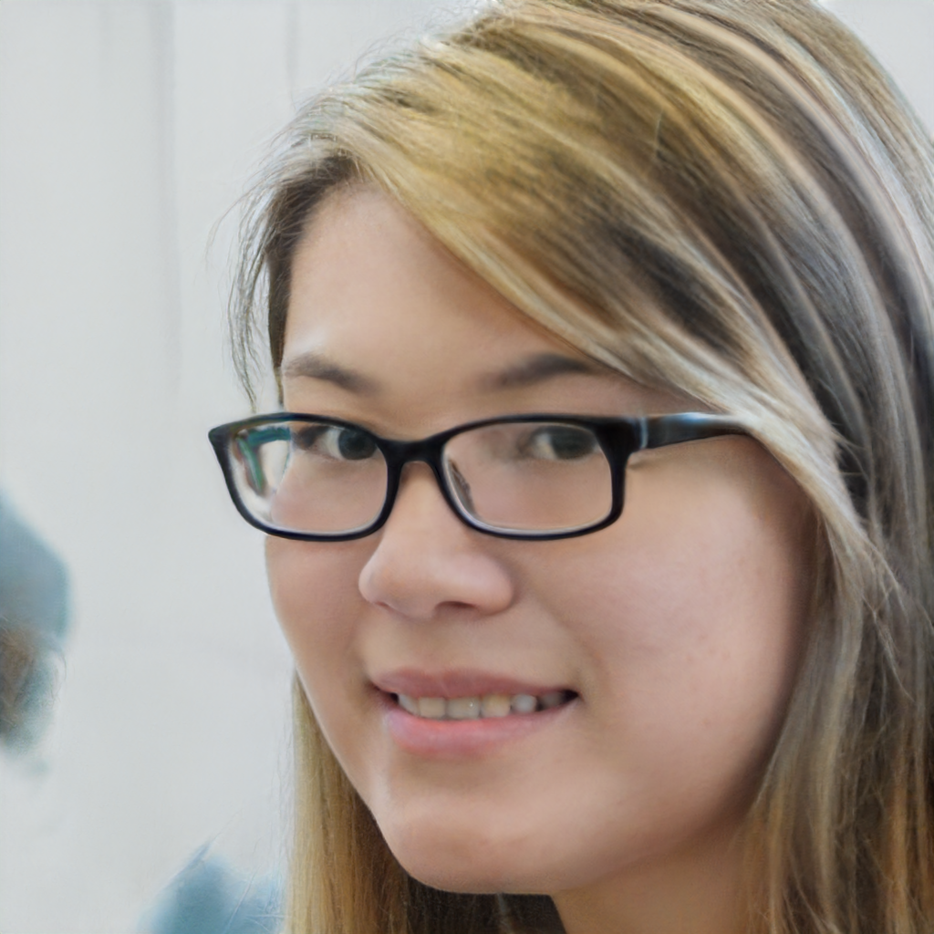
(e) StyleGAN2

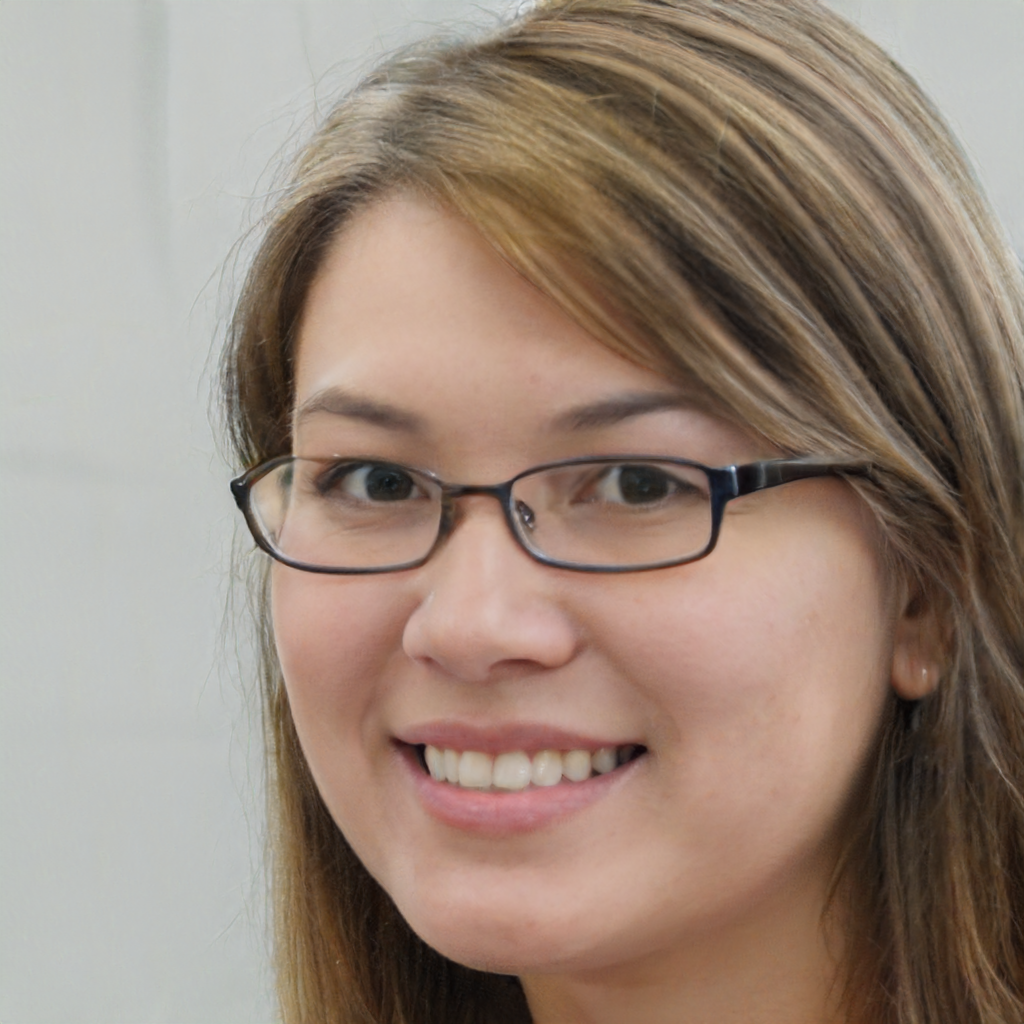
(f) StyleGAN2^∗

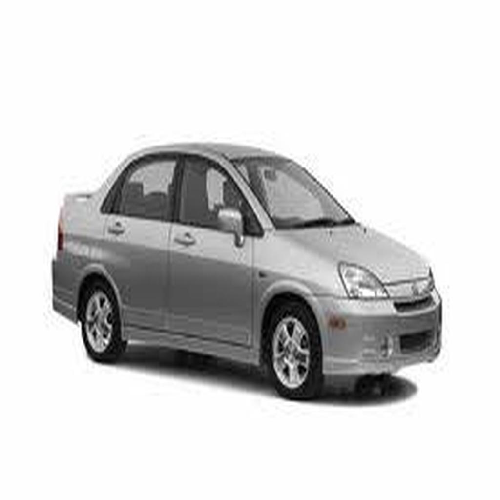
(g) StanfordCars

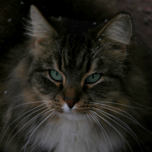
(h) AFHQv2-Cats

Figure 1: Dataset samples. The first row illustrates the human faces datasets we use, whereas the second and third rows respectively contain samples from the datasets of synthetic face images and real non-human-face images. StyleGAN2^∗ denotes the sample obtained with 0.7 truncation.

(a) Original

(b) VerticalFlip

(c) HorizontalFlip

(d) Swirl

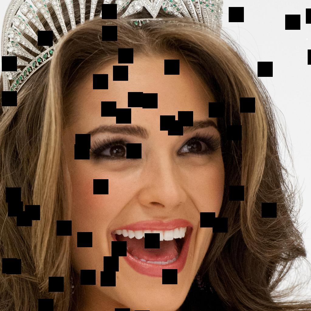
(e) RandomErase

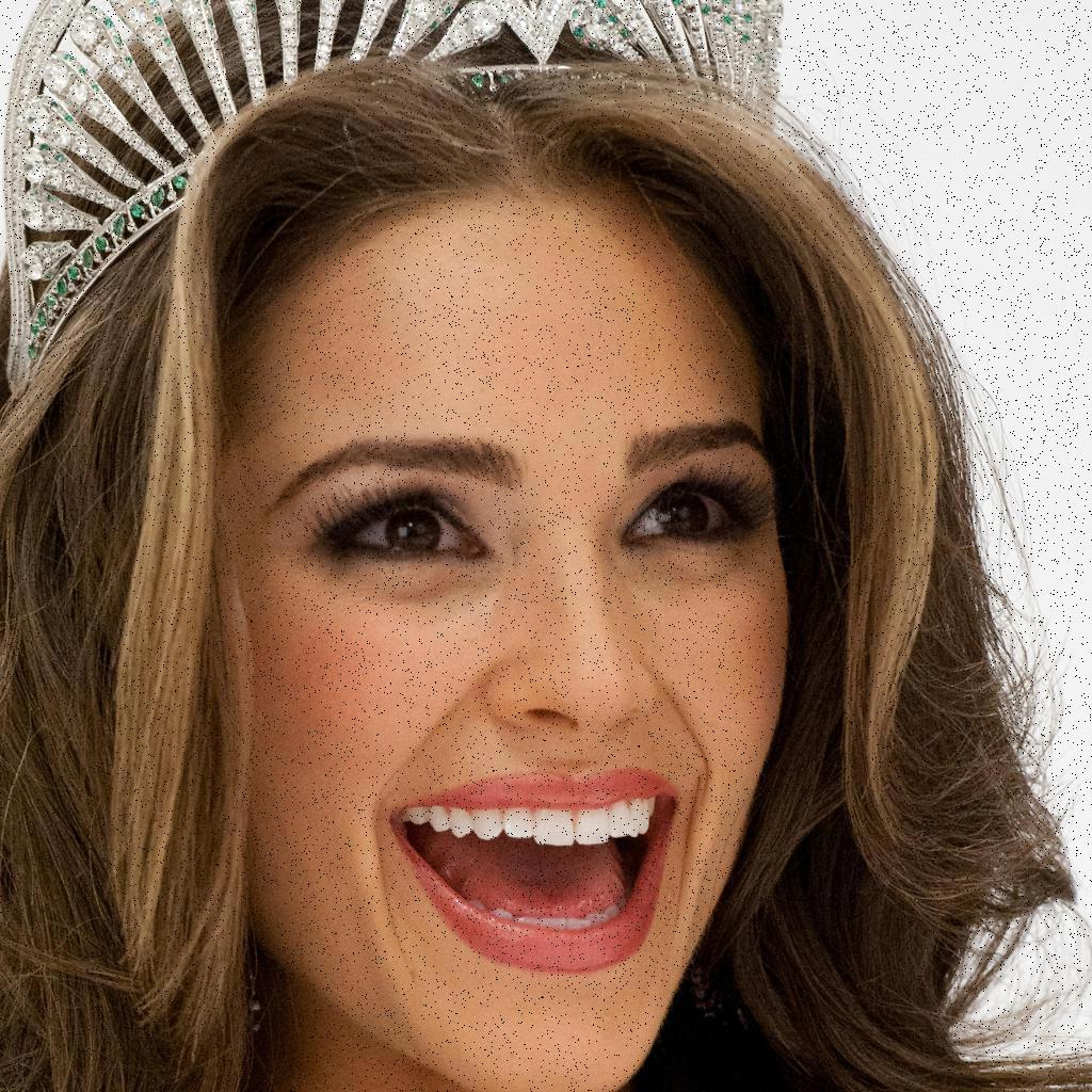
(f) SaltPepperNoise

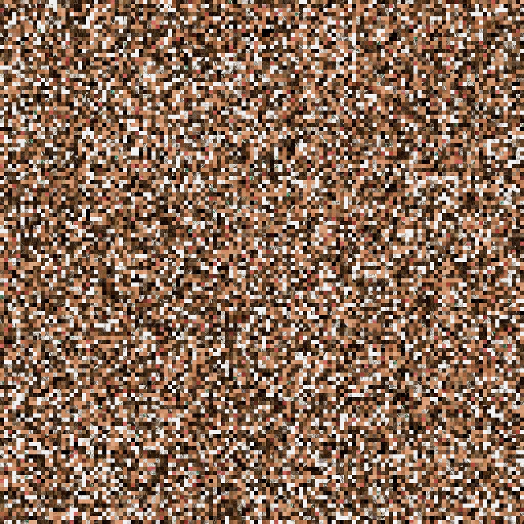
(g) Puzzle8

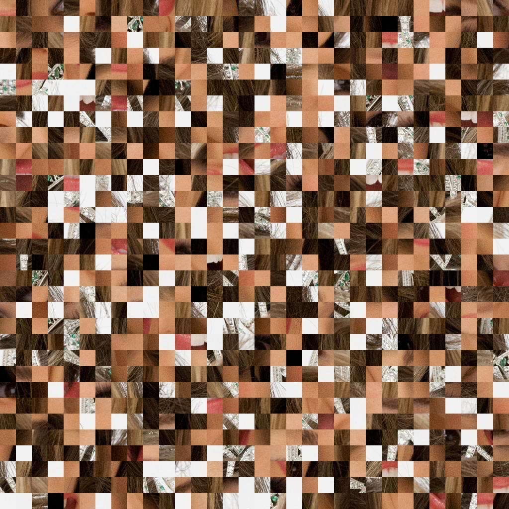
(h) Puzzle32

Figure 2: Image perturbations. We illustrate the different perturbations that we apply to images in our experimental evaluation. The original input image is shown in (a) and the remaining images illustrate each of the different types of degradation models applied to the original image.

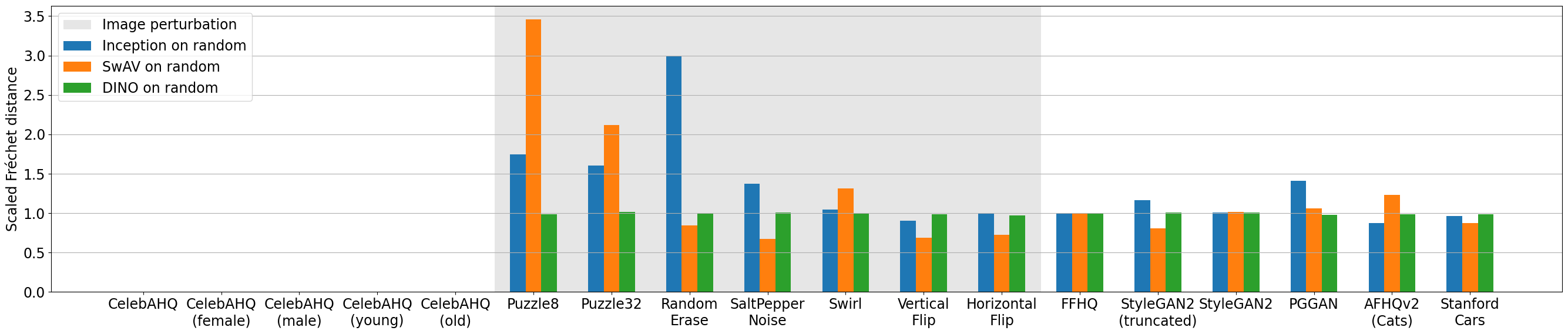
Figure 3: Rescaled Fréchet distance computed on randomly initialized Inception, SwAV and DINO features. We compute the Fréchet distances between the sets shown on the x-axis and CelebAHQ data (5k samples). For better readability, we rescale all values with a ratio that is fixed per method and determined by an independent dataset. All values that are cut off for better readability are denoted next to their corresponding bars.

We utilize several various datasets of real and synthetic images in our experiments. Image samples from the datasets are shown in Figure 1 and the datasets are detailed below, grouped into three categories.

Human face datasets: CelebAHQ contains 30’000 aligned face images. FFHQ is an improvement over former in both quality and quantity, containing 70’000 images with less bias over attributes such as gender and age. Faces is a separate face dataset of 30’000 samples we collect, preprocessed in the same way as CelebAHQ and FFHQ. To promote better fairness, we also balance our dataset across six ethnicity groups, to alleviate concerns over ethnicity biases in such datasets as FFHQ.

Synthetic datasets: For PGGAN we construct a dataset over 10’000 samples generated by a network trained on CelebAHQ. For StyleGAN2, we similarly generate 10’000 samples but using a network trained on FFHQ instead. For the truncated version of the StyleGAN2, use a truncation value of $0.7$ and we keep the random seed fixed, thus samples in truncated and untruncated datasets match each other in terms of attributes of synthetic people they contain.

Non-human-face datasets: We also utilize two datasets that do not contain images of human faces. First is AFHQv2-Cats where we utilize all 5’558 cat images from AFHQv2 dataset, which contains face images of animals obtained through a similar preprocessing as in aforementioned face datasets. The second is Stanford Cars dataset, where we utilize the test set with 8’042 samples. It is the only dataset we use where the images do not have equal width and height of 1024 pixels and we resize all images to squares as preprocessing for the networks we use in our experiments.

CelebAHQ attribute distribution: CelebAHQ provides annotations for several attributes for each image. We use two of those labels, namely ”Young” and ”Male”, to sample class-specific data for our experiments and our survey. Table I shows the distribution of the dataset with respect to these two labels, highlighting the biases of CelebAHQ. In our survey section on image correspondences we sample the images from CelebAHQ to construct image grids uniformly, such that the class distribution of all the images used in image grids match the percentages reported in Table I.

Label	Male	Female	Old	Young
Percentage	$37\%$	$63\%$	$22\%$	$78\%$

TABLE I: CelebAHQ class distributions. We show for reference the percentages of the different CelebAHQ classes used in our classification experiments.

We also explore the effects of several image perturbations on Fréchet distances in our experiments. For VerticalFlip and HorizontalFlip we mirror the image in vertical and horizontal directions, respectively. For Swirl, we apply a swirl transformation with strength of 2 and a radius of 400 pixels. For RandomErase we black out 50 randomly selected patches of size $50x50$. For SaltPepperNoise we switch up to 10’000 pixels ($0.95\%$ of a 1024x1024 image) each to black or white. For Puzzle8 and Puzzle32 we respectively divide images into patches of size 8x8 and 32x32, then shuffle them randomly. All image perturbations we use in our experiments are illustrated in Fig. 2.

II Scaling Fréchet distances

Model	$\mu$	$\sigma$
Inception (ImageNet)	4.410	0.048
SwAV (ImageNet)	2.085	0.013
DINO (Faces)	1.368	0.059
Inception (Random)	28533160.529	124058.421
SwAV (Random)	2737716.393	11397.390
DINO (Random)	15.803	0.005

TABLE II: Scaling factors per method. We list for reference all the scaling factors used for improving the readability of our benchmarking results.

There is no uniform scale over weights of different networks, trained or randomly initialized. Therefore, we normalize Fréchet distances for each model, diving it by a scaling factor calculated empirically, in order to be able to compare results from different networks more easily.

We randomly sample 5’000 samples each from CelebAHQ and FFHQ dataset and compare Fréchet distances over 10 different random seeds. Then, we use the average distance as the scaling factor for that network when we report distances elsewhere in the paper. Scaling factors used in the paper are listed in Table II, alongside the standard deviation of each run.

III Additional experimental results

We show in Fig. 3 similar benchmarking results as in our main manuscript, but with randomly initialized networks for each of the models. We observe that the results end up more or less uniform across any type of images that are outside of the CelebAHQ domain. We also note that the distances end up exploding in absolute values, and after rescaling we can see that the distances on the different CelebAHQ sets become so small that they are no longer readable. This can also be seen in Table II. Therefore, while the randomly initialized networks can still extract a certain degree of relevant features, they are not practical to use, and as we discuss in our main text the training signals are indeed useful.

Acknowledgement: Ringier, TX Group, NZZ, SRG, VSM, Viscom, and the ETH Zurich Foundation.