Second Maximum of a Gaussian Random Field and Exact ($t$-)Spacing test

Abstract

In this article, we introduce the novel concept of the second maximum of a Gaussian random field on a Riemannian submanifold. This second maximum serves as a powerful tool for characterizing the distribution of the maximum. By utilizing an ad-hoc Kac Rice formula, we derive the explicit form of the maximum’s distribution, conditioned on the second maximum and some regressed component of the Riemannian Hessian. This approach results in an exact test, based on the evaluation of spacing between these maxima, which we refer to as the spacing test.

We investigate the applicability of this test in detecting sparse alternatives within Gaussian symmetric tensors, continuous sparse deconvolution, and two-layered neural networks with smooth rectifiers. Our theoretical results are supported by numerical experiments, which illustrate the calibration and power of the proposed tests. More generally, this test can be applied to any Gaussian random field on a Riemannian manifold, and we provide a general framework for the application of the spacing test in continuous sparse kernel regression.

Furthermore, when the variance-covariance function of the Gaussian random field is known up to a scaling factor, we derive an exact Studentized version of our test, coined the $t$-spacing test. This test is perfectly calibrated under the null hypothesis and has high power for detecting sparse alternatives.

Version of July 5, 2024

1 Introduction

1.1 The $(t$-$)$spacing test and the second maximum

This paper introduces a test for the mean $m(\cdot)$ of a Gaussian random field $Z(\cdot)$, defined on a $\mathcal{C}^{2}$-compact Riemannian manifold ${M}$ of dimension $d$ without boundary, which can be decomposed as

$$\forall t\in M\,,\quad Z(t)=m(t)+\sigma X(t)\,,$$ (1.1)

where $m(\cdot)$ is any $\mathcal{C}^{2}$-function, $\sigma>0$ is the standard deviation, and $X(\cdot)$ is a centered Gaussian random field such that $\operatorname{Var}[X(t)]=1$ for every $t\in{M}$. We consider the simple global null hypothesis $\mathds{H}_{0}\,:\,\text{\textquoteleft\textquoteleft}m(\cdot)=0\,\text{''}$, even when the standard error $\sigma$ is unknown. The test investigated is the quantile $\widehat{\alpha}$ of the maximum $\lambda_{1}$ under the null defined as

$$\lambda_{1}=\max_{t\in M}\{\sigma X(t)\}$$ (1.2)

and we denote by $t_{1}\in M$ its argument maximum. This quantile is built from the distribution of $\lambda_{1}$ conditional to the values of the so-called second maximum $\lambda_{2}$ and the so-called Independent part of the Riemannian Hessian $\Omega$, under the null. Suppose, in a first step, that $\sigma$ is known, in such a case we will demonstrate that the cumulative distribution of this conditional law can be expressed as a ratio, resulting in the following expression derived from an ad-hoc Kac-Rice formula,

$$\widehat{\alpha}:=\frac{\displaystyle\int_{{\lambda_{1}}/\sigma}^{+\infty}\!\!\!\!\!\!\det(u\mathrm{Id}-\Omega/\sigma)\varphi(u)\,\mathrm{d}u}{\displaystyle\int_{{\lambda_{2}}/\sigma}^{+\infty}\!\!\!\!\!\!\det(u\mathrm{Id}-\Omega/\sigma)\varphi(u)\,\mathrm{d}u}\,,$$ (1.3)

where $\varphi(\cdot)$ is the standard Gaussian density and $\mathrm{Id}$ the identity matrix.

We will show the exactness of this test, meaning that $\widehat{\alpha}$ is uniformly distributed on the interval $(0,1)$ under the null hypothesis. It demonstrates that one minus the ratio (1.3) represents the cumulative distribution function (CDF) of the law of $\lambda_{1}$ conditional to $\lambda_{2}$ and $\Omega$, under the null hypothesis. Small values of $\widehat{\alpha}$ indicate that the maximum $\lambda_{1}$ is abnormally large compared to the value of the second maximum $\lambda_{2}$, making $\widehat{\alpha}$ interpretable as a $p$-value. This test is referred to as the “spacing test”. The second maximum is defined as

$$\lambda_{2} \in\arg\max_{s\neq t_{1}\in M}\,\{\sigma X^{|t_{1}}(s)\}\,,$$ (1.4)

$$\text{ with, for }s\neq t\,,\ X^{|t}(s) :=\frac{X(s)-c(s,t)\,X(t)-\nabla_{t}c(s,t)^{\top}\Lambda_{2}^{-1}(t)\nabla X(t)}{1-c(s,t)}$$

where $c(\cdot,\cdot)$ is the variance-covariance function of $X(\cdot)$ and $\Lambda_{2}(t):=\operatorname{Var}[\nabla X(t)]$, the formal definition will be given in Section 2.1. Note that $X^{|t}(s)$ is a normalisation of the remainder of the regression of $X(s)$ w.r.t. $(X(t),\nabla X(t))$. An example of the second maximum in the rank-one tensor detection case, referred to as Spiked tensor PCA, is illustrated in Figure 1 and developed in Section 5.2.

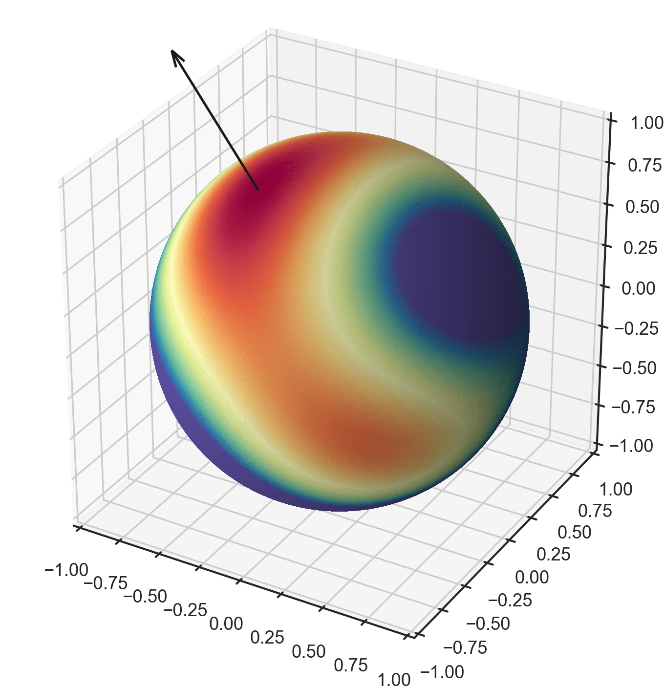
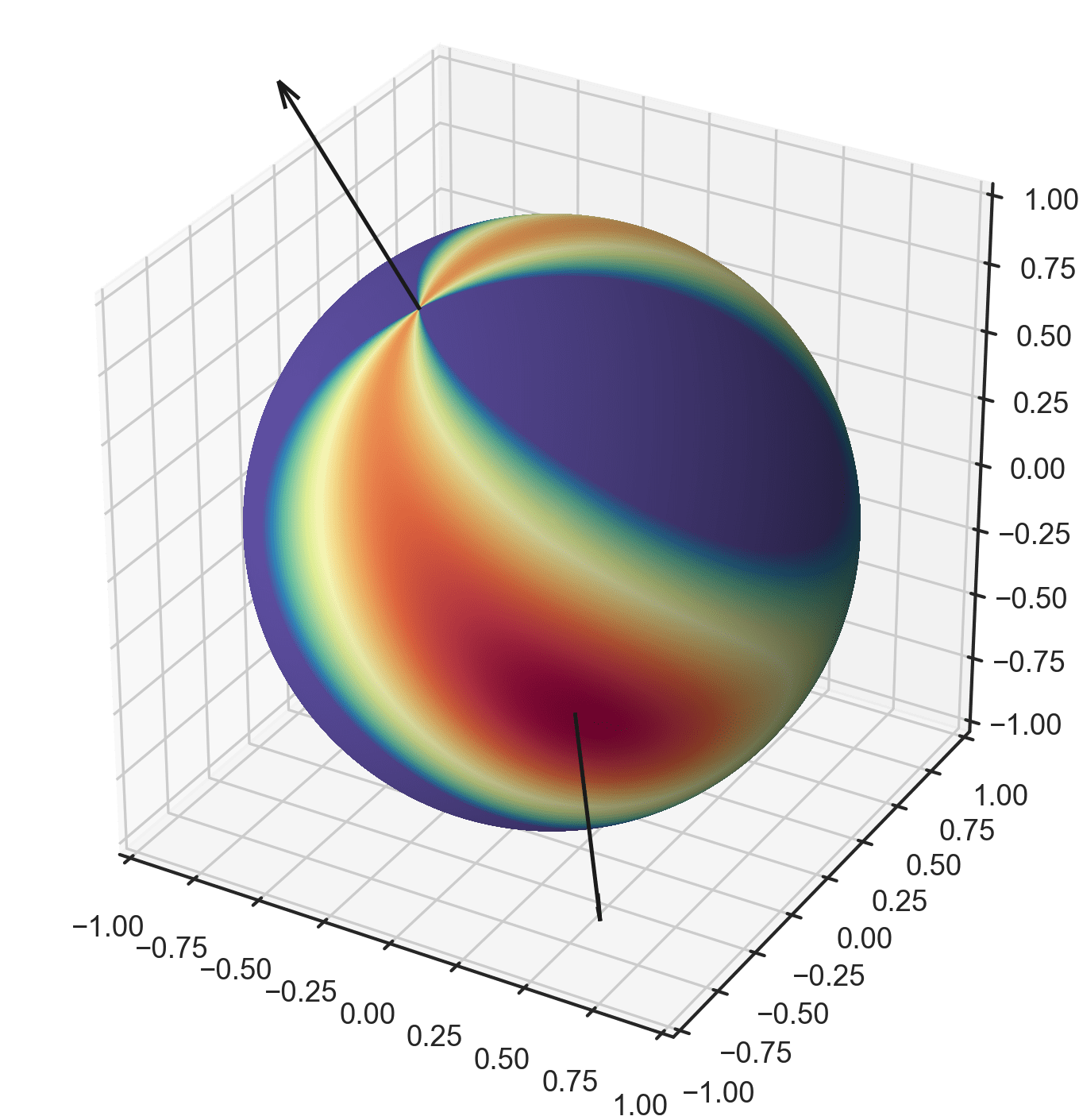
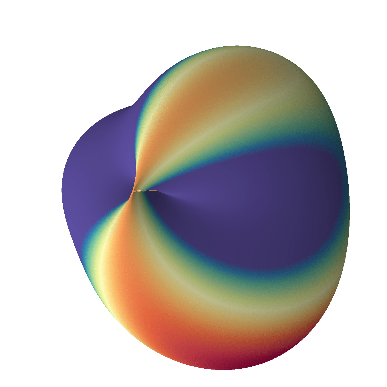
Figure 1: [Spiked tensor PCA, Section 5.2, example 1/4] The first eigenvector (resp. first eigenvalue) of a Gaussian symmetric tensor (arrow in the left panel) is the arg maximum (resp. maximum, $\lambda_{1}$) of some Gaussian homogeneous polynomial $X(\cdot)$. The second eigenvector (resp. second maximum, $\lambda_{2}$), represented by an arrow in the middle panel, is the arg maximum of $X^{|t_{1}}(\cdot)$, some regression of $X(\cdot)$. A volumic view of $X^{|t_{1}}(\cdot)$ is given in the right panel, the height of the surface around the sphere is given by the value of the random field. We witness that a singularity, referred to as the helix, appears at point $t_{1}$. A thoroughfully study of this helix will be given in this paper.

Furthermore, we will show how to achieve the same result when the variance $\sigma^{2}$ is unknown using an estimation $\widehat{\sigma}^{2}$ built from the Karhunen-Loève expansion of $X^{|t_{1}}(\cdot)$, see the right panel of Figure 1 for an illustration of this random field in the case of rank-one tensor detection. We refer to this test as the $t$-spacing test which detects abnormally large spacing between $\lambda_{1}/\widehat{\sigma}$ and $\lambda_{2}/\widehat{\sigma}$. Note that $\lambda_{1}$ and $\lambda_{2}$ are the same for the spacing and the $t$-spacing test, and these values can be computed without knowing $\sigma$. These results are supported by numerical experiments as illustrated in Figure 2.

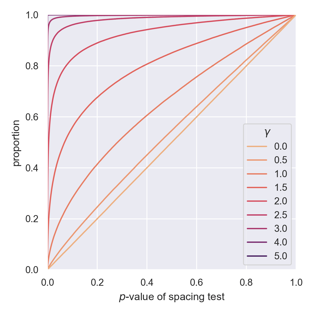
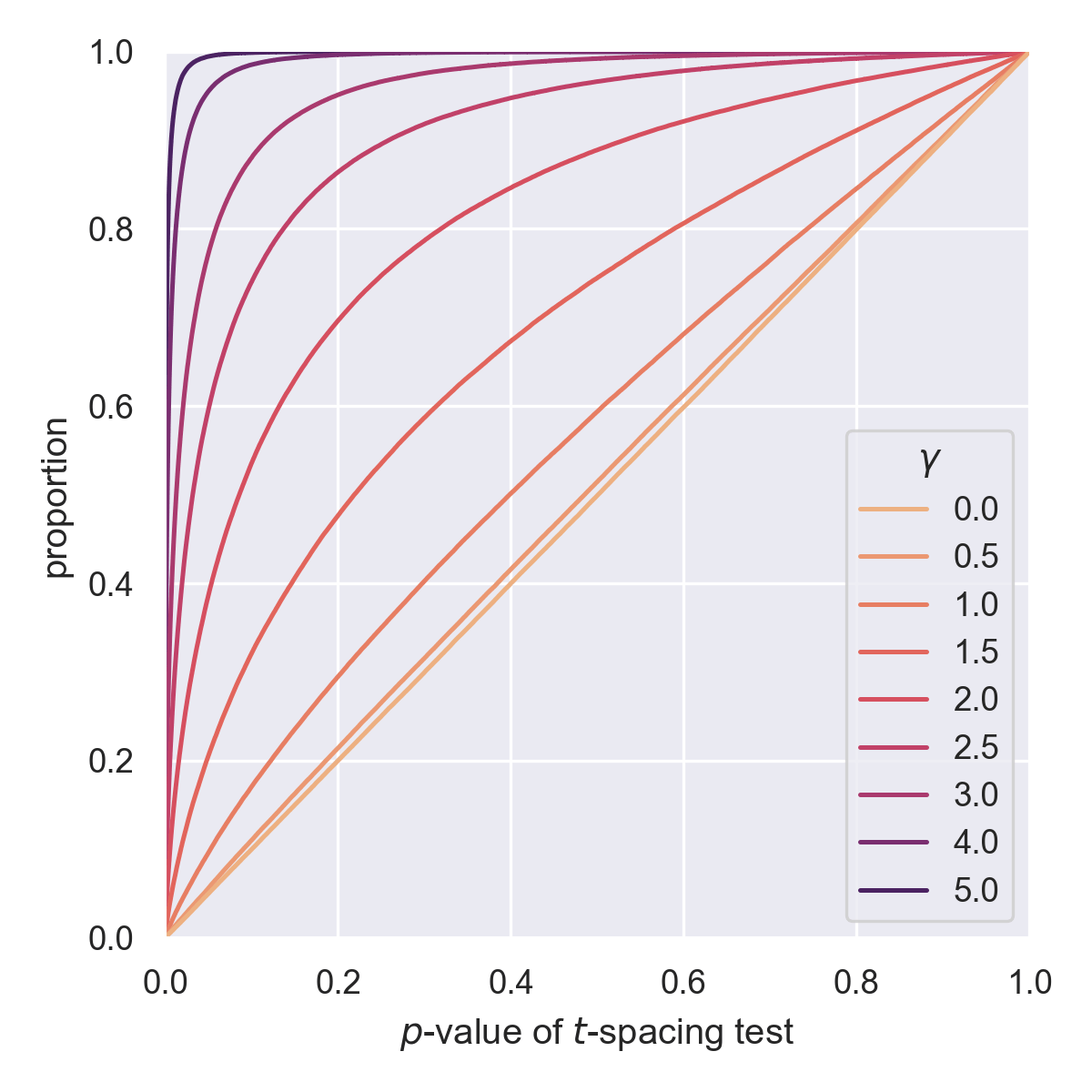
Figure 2: [Spiked tensor PCA, Section 5.2, example 2/4] The CDFs of the $p$-value of ($t$-)spacing tests over $250,000$ Monte-Carlo samples for each value of $\gamma$. Note that these tests are perfectly calibrated under the null hypothesis, for which $\gamma=0$. The parameter $\gamma$ is a scaling factor of eigenvalue of the rank-one tensor to be detected. The value $\gamma=1$ corresponds to the so-called phase transition in Spiked tensor PCA as presented in Perry et al., (2020, Theorem 1.3). In the $t$-spacing test, the variance $\sigma$ has been estimated on $X^{|t_{1}}(\cdot)$.

1.2 Detecting one sparse alternatives in continuous sparse kernel regression

Our test is perfectly calibrated for all $\mathcal{C}^{2}$-mean $m(\cdot)$. But, we expect this test to have high power on $s$-sparse alternatives of the form

$$m(\cdot)=\sum_{k=1}^{s}\lambda_{0,k}c(\cdot,t_{0,k})\,,$$

and we denote one-sparse alternatives by

$$\mathds{H}_{1}(t_{0},\lambda_{0})\,:\,\text{\textquoteleft\textquoteleft}\,m(\cdot)=\lambda_{0}c(\cdot,t_{0})\,\text{''}\,,$$ (1.5)

for some $\lambda_{0}\neq 0$ and $t_{0}\in M$ unknown. Indeed, we will show that the maxima $\lambda_{1}$ and $\lambda_{2}$ correspond to the so-called knots of the Continuous LARS algorithm and are then related to continuous kernel sparse regression, see Section 1.3.3. We illustrate this phenomenon in Figure 3 in the case of Spiked tensor PCA.

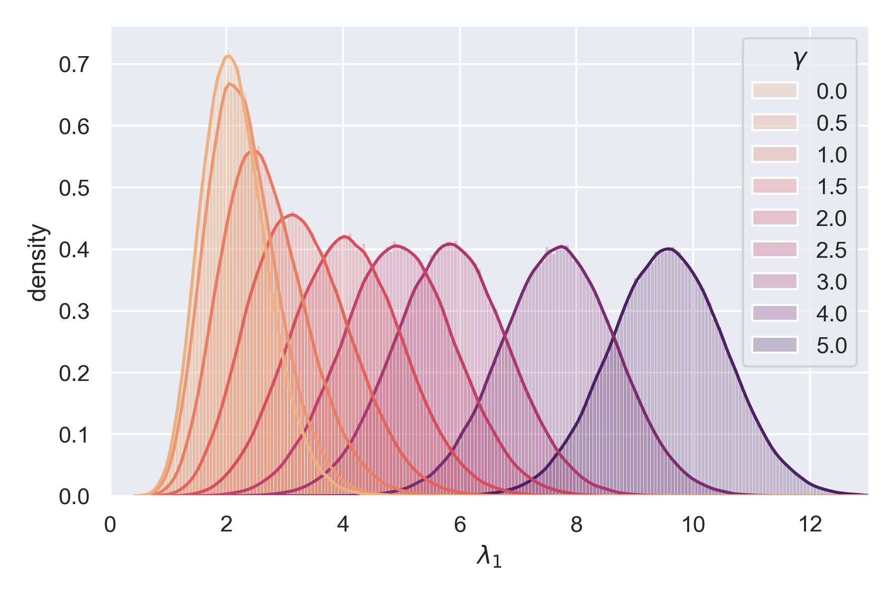
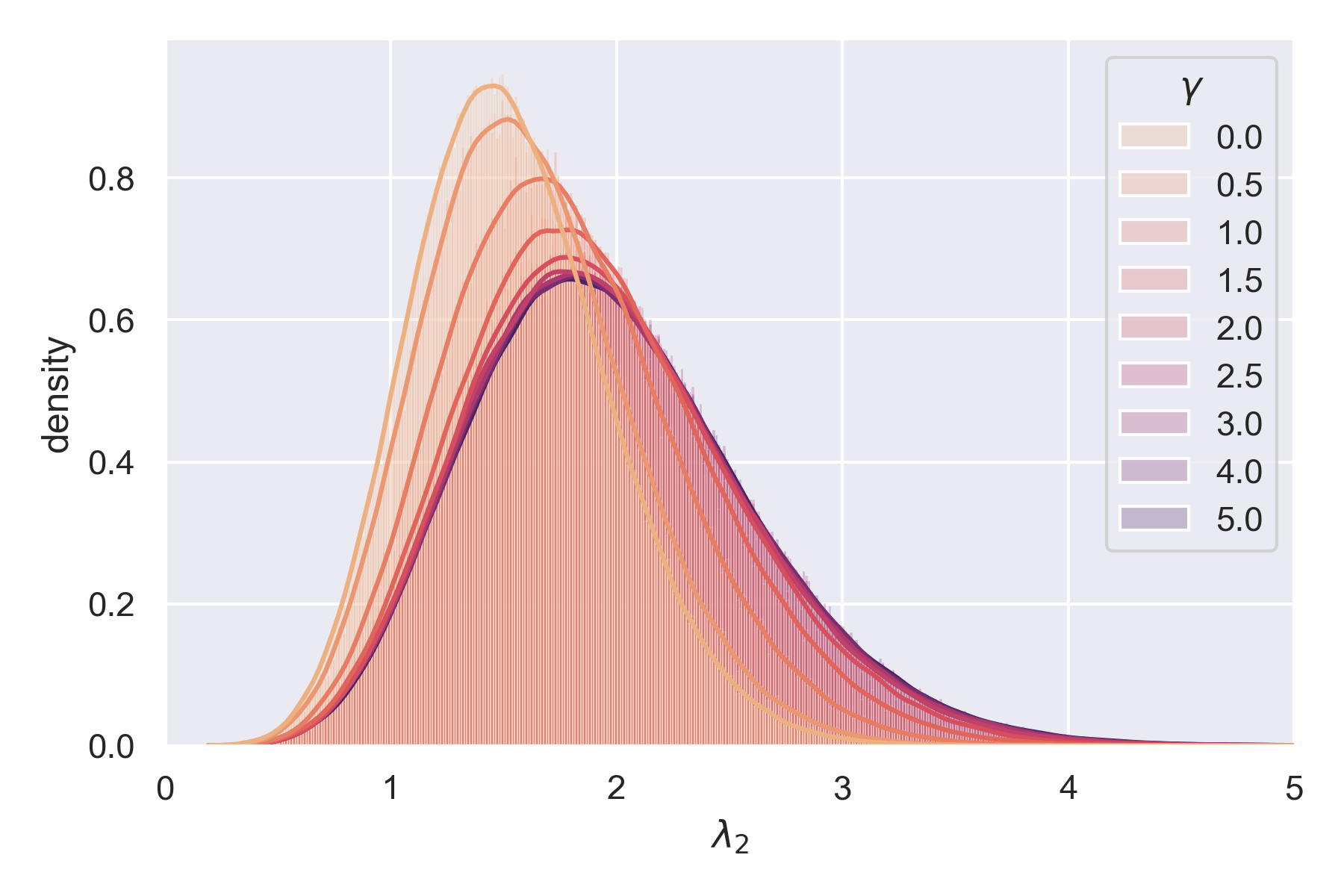
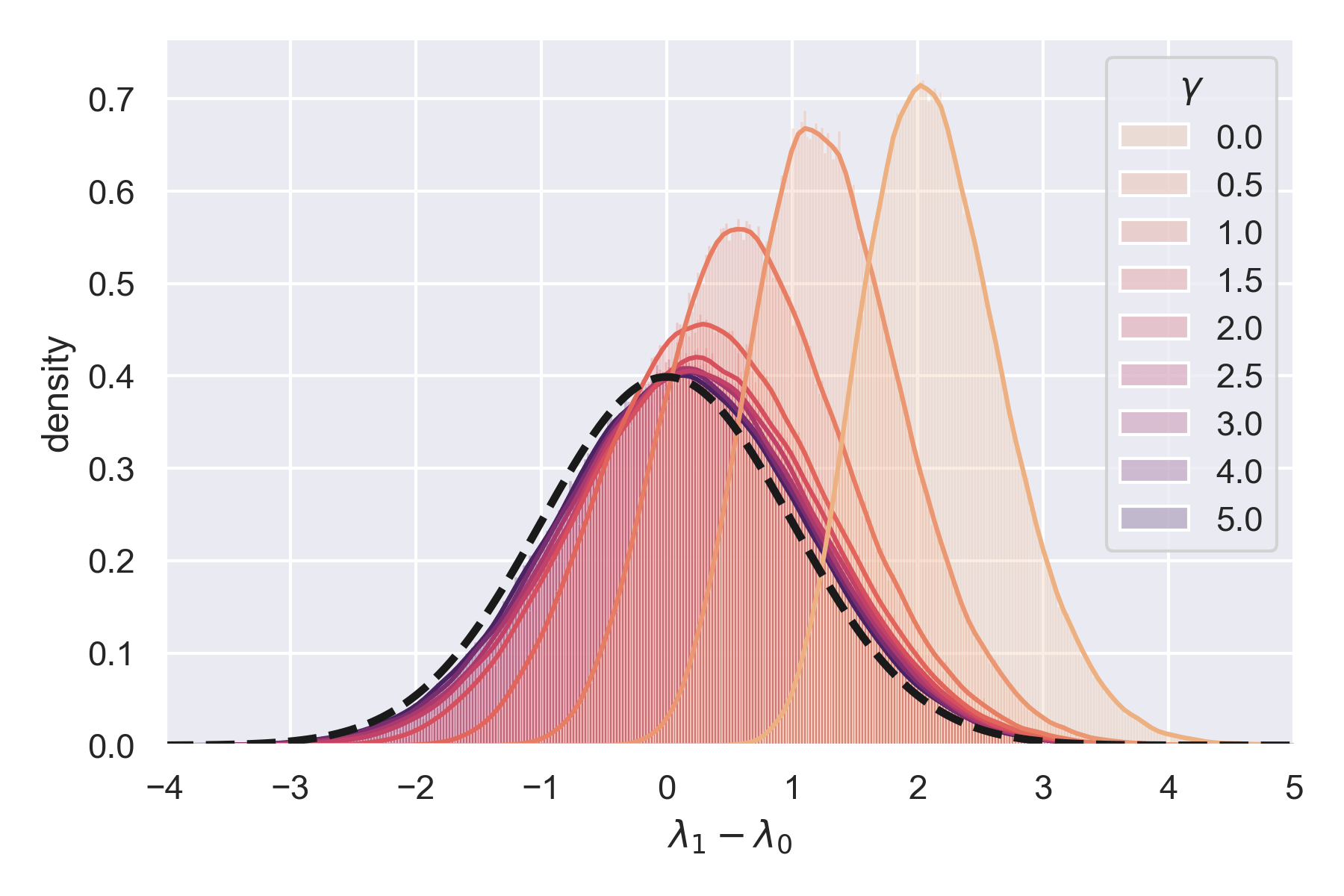
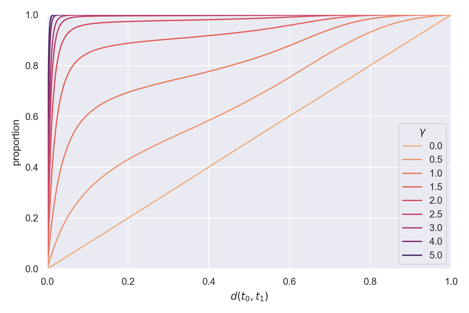
Figure 3: [Spiked tensor PCA, Section 5.2, example 3/4] The PDFs of the maxima $\lambda_{1},\lambda_{2}$ and the CDF of the distance $\mathrm{d}(t_{0},t_{1})$ over $250,000$ Monte-Carlo samples for each value of the parameter $\gamma$. The alternative is given by $t_{0}$ fixed and $\lambda_{0}=\gamma\times\sigma\sqrt{3\log 3+3\log\log 3}\simeq 0.684\gamma\sigma$ where $\gamma=1$ corresponds to the so-called phase transition in Spiked tensor PCA as presented in Perry et al., (2020, Theorem 1.3). The distance $\mathrm{d}(t_{0},t_{1})$ is normalized so that it is uniformly distributed on $(0,1)$ if $t_{1}$ is uniformly distributed on the sphere (e.g., $\gamma=0$).

In Figure 3, the alternative is given by $\lambda_{0}=\gamma\times\sigma\sqrt{3\log 3+3\log\log 3}$ where $\gamma=1$ corresponds to the so-called phase transition in Spiked tensor PCA as presented in Perry et al., (2020, Theorem 1.3). The top left panel shows that $\lambda_{1}$ is stochastically increasing as $\gamma$ increases while the top right panel shows that the distribution of $\lambda_{2}$ remains unchanged for moderate values of $\gamma$, say $\gamma\geq 2$. It illustrates that the spacing between $\lambda_{1}$ and $\lambda_{2}$ grows linearly with $\gamma$. In the moderate regime, the bottom left panel shows that $\lambda_{1}$ is distributed as a Gaussian with mean $\lambda_{0}$ and variance $\sigma^{2}$ (dashed black line), which is the distribution of $\sigma X(t_{0})$ under $\mathds{H}_{1}(t_{0},\lambda_{0})$. The bottom right panel shows that $t_{1}\simeq t_{0}$, for moderate values of $\gamma$. It illustrates that $(t_{1},\lambda_{1})$ is weakly close to the distribution of $(t_{0},\sigma X(t_{0}))$, the ($t$-)spacing tests detect the alternative $\mathds{H}_{1}(t_{0},\lambda_{0})$. We leave the proof of this phenomenon for future work.

1.3 A general framework related to continuous kernel regression

1.3.1 The four conditions on the Gaussian random field

We start by giving the assumptions of the Gaussian random field $X(\cdot)$ that we will invoke along this paper. We consider a real valued Gaussian random field $X(\cdot)$ defined on a $\mathcal{C}^{2}$ compact Riemannian manifold ${M}$ of dimension $d$ without boundary. We recall that $c(\cdot,\cdot):{M}\times{M}\to{\mathds{R}}$ denotes its variance-covariance function.

Assumption $\bf(A_{1\text{-}4})$ We assume that

$$\circ\ \text{the {paths of $X(\cdot)$ are $\mathcal{C}^{2}$ almost surely}}; \bf A_{1}$$ ()

$$\circ\ \operatorname{\mathds{E}}[X(t)]=0\text{ and }\operatorname{Var}[X(t)]=1\text{, for every }t\in{M}; \bf A_{2}$$ ()

$$\circ\ \forall s\neq t\,,\ c(s,t)<1; \bf A_{3}$$ ()

$$\circ\ \text{for every }t\in{M},\text{ the gradient }\nabla X(t)\text{ has a non-degenerate Gaussian distribution}\,. \bf A_{4}$$ ()

The variance-covariance matrix of the Gaussian tangent vector $\nabla X(t)$ is denoted by $\Lambda_{2}(t)$, which is invertible by Assumption ($\bf A_{4}$).

1.3.2 A continuous regression framework for the spacing test

General framework

We consider the following regression problem given by

$$Y=\lambda_{0}\psi_{t_{0}}+\sigma W\,,$$ (1.6)

where $\lambda_{0}\in\mathds{R}$, $t_{0}\in\mathrm{M}$ are unknown parameters; $\sigma$ is the standard deviation; $(E,\langle\cdot,\cdot\rangle_{E})$ is any Euclidean space; $\psi\,:\,t\in M\mapsto\psi_{t}\in E$; $W\in E$ is a centered Gaussian vector with variance-covariance matrix $\mathrm{Id}_{E}$. The feature map $\psi$ satisfies the following Assumptions $\bf(B_{1\text{-}6})$:

$$\circ\ \psi\text{ is a $\mathcal{C}^{3}$-function}; \bf B_{1}$$ ()

$$\circ\ \forall t\in M\,,\ \|\psi_{t}\|_{E}^{2}=1; \bf B_{2}$$ ()

$$\circ\ \forall t\in M\,,\ \forall s\in M\setminus\{t\}\,,\ \langle\psi_{s},\psi_{t}\rangle_{E}<1; \bf B_{3}$$ ()

$$\circ\ \forall t\in M\,,\ \text{$J\psi_{t}{J\psi_{t}}^{\top}$ has full rank $d$}; \bf B_{4}$$ ()

$$\circ\ \text{the span of $\{\psi_{t}\ :\ t\in M\}$ has dimension $m$ such that $m>d+1$}; \bf B_{5}$$ ()

$$\circ\ \forall t\in M\,,\ \exists s\in M\ \text{s.t.}\ \psi_{t}=-\psi_{s}; \bf B_{6}$$ ()

where $J\psi_{t}$ is the Jacobian matrix of $\psi_{t}$ and ${J\psi_{t}}^{\top}$ its transpose. In the next paragraph, we will see that $X(t)=\langle W,\psi_{t}\rangle_{E}$ and

$$\forall s,t\in M\,,\quad c(s,t)=\langle\psi_{s},\psi_{t}\rangle_{E}\,.$$

One can check that ($\bf B_{1}$) implies ($\bf A_{1}$), ($\bf B_{2}$) is equivalent to ($\bf A_{2}$), ($\bf B_{3}$) is equivalent to ($\bf A_{3}$), ($\bf B_{4}$) is equivalent to ($\bf A_{4}$), and ($\bf B_{5}$) is equivalent to the forthcoming Assumption ($\bf A_{5}$).

Remark 1 (Spiked tensor PCA, Section 5.2).

In Figures 1, 2 and 3, we considered, as an example, the detection of a rank one $3$-way symmetric tensor. We consider the sphere $\mathrm{M}=\mathds{S}^{2}$. The Euclidean space of $3$-way symmetric tensors of size $3\times 3\times 3$ is denoted by $(E,\langle\cdot,\cdot\rangle_{E})$ with dimension $m=10$, and

$$\psi_{t} :=t^{\otimes 3}=(t_{i}t_{j}t_{k})_{1\leq i,j,k\leq 3\,,}$$

$$X(t) :=\langle W,\psi_{t}\rangle_{E}=\sum_{ijk}t_{i}t_{j}t_{k}W_{ijk}\,,$$

where $W$ is an order $3$ symmetric tensor defined using symmetry and the following independent terms,

$$\circ\ W_{iii}\text{ of variance }1;\text{ there are }3\text{ principal diagonal terms},i\in[3];$$

$$\circ\ W_{iij}\text{ of variance }1/3;\text{ there are }6\text{ sub-diagonals terms},1\leq i\neq j\leq 3;$$

$$\circ\ W_{123}\text{ of variance }1/6;\text{ there is }1\text{ off-diagonal term}\,.$$

Maximum likelihood estimator (MLE)

The Maximum Likelihood Estimator (MLE) of the couple $(\lambda_{0},t_{0})$ is given by

$$\operatorname*{arg\,min}_{(\lambda,t)}\Big{\{}\frac{1}{2}\big{\|}Y-\lambda\psi_{t}\big{\|}_{E}^{2}\Big{\}}\,.$$

Minimization with respect to $\lambda$ is straightforward under Assumptions ($\bf B_{2}$) and ($\bf B_{6}$) leading to

$$\operatorname*{arg\,min}_{t}\min_{\lambda}\Big{\{}\frac{1}{2}\big{\|}Y-\lambda\psi_{t}\big{\|}_{E}^{2}\Big{\}}=\operatorname*{arg\,max}_{t}\,\langle Y,\psi_{t}\rangle_{E}\,.$$ (1.7)

Now consider the Gaussian random field $Z(t):=\langle Y,\psi_{t}\rangle_{E}$, referred to as the profile likelihood. The argument maximum (resp. the maximum) of $Z(\cdot)$ is exactly the MLE of $t_{0}$ (resp. of $\lambda_{0}$) by (1.7), namely

$$\lambda^{\mathrm{MLE}}=\max Z\quad\text{and}\quad t^{\mathrm{MLE}}=\operatorname*{arg\,max}Z\,.$$

By (1.6), note that we uncover the decomposition (1.1) and the alternative hypothesis (1.5) as

$$Z(t)=\langle Y,\psi_{t}\rangle_{E}=\lambda_{0}\langle\psi_{t_{0}},\psi_{t}\rangle_{E}+\sigma\langle W,\psi_{t}\rangle_{E}=\lambda_{0}c(t_{0},\cdot)+\sigma X(t)\,,$$ (1.8)

where $X(t):=\langle W,\psi_{t}\rangle_{E}$ and $m(\cdot)=\lambda_{0}c(t_{0},\cdot)$.

Remark 2.

Assumption ($\bf B_{6}$) ensures that the profile likelihood is given by $Z(\cdot)$, see (1.7).

1.3.3 Parallel with the LARS algorithm

Discrete LARS

The LARS algorithm has been introduced in Efron et al., (2004) and has been widely used in statistics for variable selection. Given an observation $Y\in\mathds{R}^{n}$ and $p$ covariates $(\psi_{t})_{t=1}^{p}$, the Least Angle Regression (LARS) algorithm is a forward stepwise variable selection algorithm giving a sequence $(\lambda_{i},t_{i})$ of the so-called knots. The first knot $(\lambda_{1},t_{1})$ is the maximum and the argument maximum of the maximal absolute correlation between the observation and the covariates. Hence, the first step of the LARS aims at maximizing

$$\lambda_{1}=\max_{1\leq t\leq p}|\langle Y,\psi_{t}\rangle_{\mathds{R}^{n}}|\quad\text{and}\quad t_{1}=\arg\max_{1\leq t\leq p}|\langle Y,\psi_{t}\rangle_{\mathds{R}^{n}}|\,.$$ (1.9)

We define the so-called residual by, for all $\lambda\leq\lambda_{1}$,

$$\forall t\in\{1,\ldots,p\}\,,\quad Z^{\lambda}(t):=\langle Y-(\lambda_{1}-{\lambda})\psi_{t_{1}},\psi_{t}\rangle_{\mathds{R}^{n}}\,,$$ (1.10)

The second knot is defined by

$$\lambda_{1}-\lambda_{2}:=\inf\big{\{}\varepsilon>0\ :\ \exists t\neq t_{1}\text{ s.t. }Z^{\lambda_{1}-\varepsilon}(t)\geq\lambda_{1}-\varepsilon\big{\}}\,.$$ (1.11)

The second knot $(\lambda_{2},t_{2})$ is built so that $t_{1}$ is the unique argument maximum of $Z^{\lambda}(\cdot)$ for $\lambda_{2}<\lambda\leq\lambda_{1}$ and that there exists a second point, say $t_{2}\neq t_{1}$, such that $Z^{\lambda_{2}}(t_{1})=Z^{\lambda_{2}}(t_{2})=\lambda_{2}$.

Continuous LARS

The continuous LARS has been pioneered investigated in Azaïs et al., (2020) for continuous sparse regression from Fourier measurements, see Section 5.4 for further details. We introduce the continuous LARS in a general setting as follows. The first knot $(\lambda_{1},t_{1})$ is the maximum and the argument maximum of the maximal absolute correlation between the observation $Y\in E$ and $\psi_{t}\in E$, the features. Hence, the first step of the LARS aims at maximizing

$$\lambda_{1}=\max_{t\in{M}}|\langle Y,\psi_{t}\rangle_{E}|\quad\text{and}\quad t_{1}=\arg\max_{t\in{M}}|\langle Y,\psi_{t}\rangle_{E}|\,.$$ (1.12)

Under ($\bf B_{6}$), note that $\max_{t\in{M}}|Z(t)|=\max_{t\in{M}}Z(t)$, where $Z(t)=\langle Y,\psi_{t}\rangle_{E}$. Therefore, the definition of $\lambda_{1}$ given in (1.2) coincides with the aforementioned definition of $\lambda_{1}$. One can chose $t_{1}$ being the unique argument maximum of $Z(\cdot)$, by ($\bf B_{1}$) and ($\bf B_{3}$) (see also (2.4) in Lemma 1). We define the so-called residual by, for all $\lambda\leq\lambda_{1}$,

$$Z^{\lambda}(t):=\langle Y-(\lambda_{1}-{\lambda})\psi_{t_{1}},\psi_{t}\rangle_{E}=Z(t)-(\lambda_{1}-{\lambda})c(t,t_{1})\,,$$ (1.13)

where $c(s,t)=\langle\psi_{s},\psi_{t}\rangle_{E}$. Again, under ($\bf B_{6}$), note that $\max_{t\in{M}}|Z^{\lambda}(t)|=\max_{t\in{M}}Z^{\lambda}(t)$. Moreover, one can check that $Z^{\lambda}(t_{1})=\lambda$. The second knot is defined by

$$\lambda_{1}-\lambda_{2}:=\inf\big{\{}\varepsilon>0\ :\ \exists t\neq t_{1}\text{ s.t. }Z^{\lambda_{1}-\varepsilon}(t)\geq\lambda_{1}-\varepsilon\big{\}}\,.$$ (1.14)

The second knot $(\lambda_{2},t_{2})$ is built so that $t_{1}$ is the unique argument maximum of $Z^{\lambda}(\cdot)$ for $\lambda_{2}<\lambda\leq\lambda_{1}$ and that there exists a second point, say $t_{2}\neq t_{1}$, such that $Z^{\lambda_{2}}(t_{1})=Z^{\lambda_{2}}(t_{2})=\lambda_{2}$. Now observe that, for all $t\neq t_{1}\in{M}$ and all $\lambda$,

$$Z^{\lambda}(t)\leq\lambda\ \Leftrightarrow\ Z(t)-\lambda_{1}c(t,t_{1})\leq\lambda(1-c(t,t_{1}))\ \Leftrightarrow\ \frac{Z(t)-Z(t_{1})c(t,t_{1})}{1-c(t,t_{1})}\leq\lambda\ \Leftrightarrow\ Z^{|t_{1}}(t)\leq\lambda\,,$$

where $Z^{|t_{1}}(t)$ is defined as in (1.4), taking into account that the gradient is vanishing at point $t_{1}$. We uncover that $(\lambda_{2},t_{2})$ is the second knot of the LARS where

$$\lambda_{2}=\max_{t\in{M}\setminus\{t_{1}\}}Z^{|t_{1}}(t)\quad\text{and}\quad t_{2}=\max_{t\in{M}\setminus\{t_{1}\}}Z^{|t_{1}}(t)\,.$$ (1.15)

Note that the definition of $\lambda_{2}$ in (1.4) is equivalent to the aforementioned definition of $\lambda_{2}$ (this is also true for the argument maximum). This paper gives the distribution of $\lambda_{1}$ (first knot of the continuous LARS) conditional to $(\lambda_{2},\Omega)$ (second knot of the continuous LARS and independent part of the Hessian at the first knot) under the null hypothesis.

1.4 Contributions and outline

This paper investigates the notion of second maximum $\lambda_{2}$ of a Gaussian random field. The definition of second maximum originates from continuous LARS, see Section 1.3.3, and can be used in a Kac-Rice formula to compute the conditional law of the maximum $\lambda_{1}$ with respect to $\lambda_{2}$ and the so-called independent part of the Hessian $\Omega$. The second maximum is the maximum of a random field $\sigma X^{|t_{1}}(\cdot)$ with a singularity at point $t_{1}$. A first contribution establishes a link between the eigen-decomposition of $\Omega$ and the directional limiting values of $\sigma X^{|t_{1}}(\cdot)$ at the singularity point $t_{1}$. see Lemma 3. The second contribution is a Kac-Rice type formula, see Appendix B, that gives the conditional law in an explicit form, see Theorem 1. From this point, we derive an exact test based on the spacing between $\lambda_{1}$ and $\lambda_{2}$, see Theorem 2. We introduce an estimation of the variance $\widehat{\sigma}$ in Section 4.2, that can be used in a Kac-Rice formula and lead to the conditional law of $\lambda_{1}/\widehat{\sigma}$ in Proposition 7. We derive an exact test based on the spacing between $\lambda_{1}/\widehat{\sigma}$ and $\lambda_{2}/\widehat{\sigma}$ which can be used when the variance $\sigma^{2}$ is unknown, see Theorem 3. The reader may consult https://github.com/ydecastro/tensor-spacing/ for further details on the numerical experiments of this paper.

The paper is organized as follows. Section 2 introduces the second maximum of a Gaussian random field. Section 2.3 gives an ad-hoc Kac-Rice formula for the conditional law of $\lambda_{1}$ with respect to $\lambda_{2}$ and $\Omega$. Section 3 gives the exact tests based on the spacing between $\lambda_{1}$ and $\lambda_{2}$ and the spacing between $\lambda_{1}/\widehat{\sigma}$ and $\lambda_{2}/\widehat{\sigma}$. Section 4.4 introduces the estimation of the variance $\widehat{\sigma}$ from the Karhunen-Loève expansion of $X^{|t_{1}}(\cdot)$. Section 5 gives the parallel with continuous sparse kernel regression.

1.5 Related works

The first paper which considers Kac-Rice formula on manifolds, in fact the sphere and the Stiefel Manifold, is Azaïs and Wschebor, (2004). The subject is developed in Adler and Taylor, (2009) and Azaïs and Wschebor, (2009). The article Auffinger and Ben Arous, (2013) considers the high dimensional sphere. A new set of hypotheses and proofs is also given in Armentano et al., (2023).

The Kac-Rice formula is also used in Azaïs et al., (2017) for the study of the maximum of a Gaussian random field on the torus with application to the so-called Super-Resolution problem. It falls under the general theory of continuous sparse regression over the space of measures which has recently attracted a lot of attention in signal processing (Candès and Fernandez-Granda,, 2014; Duval and Peyré,, 2015) among the super-resolution community; in machine learning (De Castro et al.,, 2021); and in optimization (Chizat,, 2022). The super-resolution framework aims to recover fine scale details of an image from just a few low frequency measurements, where ideally the observation is given by a low-pass filter. It has potential applications in astronomy, medical imaging, and microscopy. The novel aspects of this body of work rely on new statistical and optimization guarantees of sparse regression over the space of measures. Initiated by the work presented in (Azaïs et al.,, 2020), one investigate the possibility of detecting a sparse object from a test on the mean $m(\cdot)$ of a Gaussian random field under a sparsity-type assumption.

General notation
$[a]$	Set of integers $\{1,\ldots,a\}$;
$A^{\top}$ $(\text{resp. }A_{i:})$	transpose of a matrix $A$ (resp. $i$-th line);
$\mathrm{Id}$	Identity matrix of dimension $d\times d$;
$\mathcal{S}_{d}$	Space of $d\times d$ symmetric matrices;
$\mathds{S}^{d-1}$	Euclidean sphere of $\mathds{R}^{d}$;
$t$ (and $s$)	Generic value for a vector on the manifold $M$;
$\mathcal{C}^{k}$	Set of $k$ times differentiable functions;
$\delta_{jk}$	Kronecker symbol;
$\mathrm{(const)}$	Positive constant which may change from line to line;
$\mathcal{D}(U\,|\,V)$	Conditional distribution of $U$ with respect to $V$;
$\operatorname{Var}(U)$	Variance matrix of a random vector $U$;
$\operatorname{Cov}(U,V)$	Covariance matrix of the random vectors $U$ and $V$;
$\varphi(\cdot)$	Standard Gaussian density in ${\mathds{R}}$;
$p_{U}(\ell)$	Density function of the random variable/vector $U$ at point $\ell$;
$\mathds{1}_{A}$ (resp. $\mathds{1}{\{A\}})$	Indicator function of condition $A$ (resp. event $A$);
$\mathrm{Leb}$	Lebesgue measure on $\mathds{R}$;
$\mathcal{U}(0,1)$	Uniform law on $(0,1)$;
$\mu\otimes\nu$	Product of measures;
Random fields
$Z(\cdot)$	Observed Gaussian random field, indexed by $M$;
$m(\cdot)$	Mean function of $Z(\cdot);$
$\sigma$	Standard error of the $Z(\cdot)$;
$X(\cdot)$	Centered Gaussian random field with unit variance;
$c(s,t)$	Covariance function of $X(\cdot)$ and $Z(\cdot)/\sigma$, $c(s,t)=\operatorname{\mathds{E}}(X(s)X(t))$;
Differential geometry
$M$	$\mathcal{C}^{2}$-compact Riemannian manifold of dimension $d$ without boundary;
$\nabla f(t)$	Riemannian gradient at point $t\in M$ of $f\,:\,M\to\mathds{R}$;
$\nabla_{t}g(s,t)$	Riemannian gradient at point $t\in M$ of $g(s,\cdot)$;
$\nabla^{2}f(t)$	Riemannian Hessian at point $t\in M$ of $f\,:\,M\to\mathds{R}$;
Continuous regression
$(E,\langle\cdot,\cdot\rangle_{E})$	Euclidean space;
$\psi$	Feature map from $M$ to $E$, $\psi\,:\,t\in M\mapsto\psi_{t}\in E$;
$\psi_{t}$	Vector $\psi(t)\in E$;
$J\psi_{t}$ (resp. ${J\psi_{t}}^{\top}$)	(resp. transpose of) Jacobian matrix of $\psi$ at point $t$;
$W$	Standard Gaussian random vector of $E$;
$\mathbf{S}_{\sigma}$ (resp. $\mathbf{T}$)	Generalized spacing test (resp. Generalized $t$-spacing test);

Table 1: List of notation: Riemannian gradients and Hessians are defined using the Levi-Civita connection. Riemannan Hessians are represented in matrix form.

2 The second maximum of a Gaussian random field

2.1 The two Gaussian regression remainders

Some useful properties are presented in the next lemma.

Lemma 1.

Under Assumption $\bf(A_{1\text{-}4})$, one has

$$\circ\ c(s,t)=\operatorname{\mathds{E}}[X(s)\,X(t)]\text{ and }c(t,t)=1;$$ (2.1)

$$\circ\ X(t)\text{ and }\nabla X(t)\text{ are independent;}$$ (2.2)

$$\circ\ \Lambda_{2}(t):=\operatorname{Var}[\nabla X(t)]=-\operatorname{Cov}[\nabla^{2}X(t),X(t)]$$ (2.3)

$$\circ\ \text{the argument maximum of }X(\cdot)\text{ is unique.}$$ (2.4)

Proof.

The first property (2.1) is equivalent to ($\bf A_{2}$). The other properties can be deduced by differentiating $c(t,t)=1$. The last statement is a consequence of Tsirelson’s theorem, see for instance Lifshits, (1983, Theorem 3). ∎

The Gaussian random field $X^{|t}(\cdot)$

We know that $X(t)$ and $\nabla X(t)$ are independent by (2.2). For a fixed point $t\in{M}$, consider the remainder of Gaussian regression of $X(s)$ with respect to $(X(t),\nabla X(t))$ given by the Gaussian random field

$$s\in{M}\mapsto X(s)-c(s,t)\,X(t)-\nabla_{t}c(s,t)^{\top}\Lambda_{2}^{-1}(t)\nabla X(t)\in\mathds{R}\,,$$

where $\nabla_{t}c(s,t)$ is the Riemannian gradient of $t\mapsto c(s,t)$. By ($\bf A_{4}$), remark that $\Lambda_{2}(t)$ is invertible. This Gaussian random field is well defined on ${M}$ and independent of $(X(t),\nabla X(t))$. Now, for $s\neq t$, set

$$X^{|t}(s):=\frac{X(s)-c(s,t)\,X(t)-\nabla_{t}c(s,t)^{\top}\Lambda_{2}^{-1}(t)\nabla X(t)}{1-c(s,t)},$$ (2.5)

that is, $X^{|t}(s)$ is a normalisation of the remainder of the regression of $X(s)$ w.r.t. $(X(t),\nabla X(t))$.

The regression of the Hessian $R(t)$

Now, consider the following regression in the space of Gaussian symmetric matrices

$$\nabla^{2}X(t)=-\Lambda_{2}(t)\,X(t)-\Lambda_{3}(t)\nabla X(t)+\widetilde{R}(t),$$ (2.6)

for some well-defined $3$-way tensor $\Lambda_{3}(t)$. It will not be necessary to give the explicit expression of $\Lambda_{3}(t)$ for our purposes, this tensor is well defined by Gaussian regression formulas. Thus, one can identify the symmetric matrix $\widetilde{R}(t)$ as the remainder of the regression of $\nabla^{2}X(t)$ on $(X(t),\nabla X(t))$. For future use, it is convenient to set

$$R(t):=\Lambda^{-\frac{1}{2}}_{2}(t)\,\widetilde{R}(t)\,\Lambda^{-\frac{1}{2}}_{2}(t)\,.$$ (2.7)

Note that $\widetilde{R}(t)$ and $R(t)$ are symmetric. The following lemma is straightforward.

Lemma 2.

For any $t\in{M}$, the Gaussian random field $X^{|t}(\cdot)$ and the Gaussian random matrix $R(t)$ are independent of $(X(t),\nabla X(t))$.

2.2 The first and second maxima, and the independent part of the Hessian

First maximum: We define the first maximum $\lambda_{1}$ of $\sigma X(\cdot)$ and its argument maximum $t_{1}$ by

$$\lambda_{1}:=\sigma X({t_{1}})\quad\mathrm{and}\quad{t_{1}}:=\operatorname*{arg\,max}_{t\in{M}}X(t).$$ (2.8)

The argument maximum is almost surely a singleton by (2.4), hence $t_{1}$ is unique almost surely.

Second maximum: We define the second maximum $\lambda_{2}$ of $\sigma X(\cdot)$ by

$$\forall t\in{M},\quad\lambda_{2}^{t}:=\sup_{s\in{M}\setminus\{t\}}\{\sigma X^{|t}(s)\}\quad\mathrm{and}\quad\lambda_{2}:=\lambda_{2}^{{t_{1}}}\,.$$ (2.9)

Independent part of the Hessian: We define the independent part of the Hessian $\Omega$ as

$$\Omega:=\sigma R({{t_{1}}})=\sigma\Lambda^{-\frac{1}{2}}_{2}({{t_{1}}})\,\widetilde{R}({{t_{1}}})\,\Lambda^{-\frac{1}{2}}_{2}({{t_{1}}})\,.$$ (2.10)

At this stage, it is not clear that $\lambda_{2}^{t}<\infty$ a.s. and how $X^{|t}(s)$ is shaped around point $t$. The next lemma gives a description of $s\mapsto X^{|t}(s)$ around point $t$ which proves that $\lambda_{2}^{t}<\infty$ almost surely. A proof of this lemma can be found in Appendix A. Note that, since ${M}$ is compact, by the Hopf–Rinow theorem, ${M}$ is geodesically complete and the exponential map exists on the whole tangent space.

Lemma 3.

Let $h$ be a nonzero vector of the tangent space at point $t$. For all $\varepsilon\neq 0$, let $s(\varepsilon):=\exp_{t}(\varepsilon h)\in{M}$ be the exponential map at $t$ given by the tangent vector $\varepsilon h$. Then, under Assumptions ($\bf A_{1}$), ($\bf A_{2}$) and ($\bf A_{4}$),

$$\lim_{\begin{subarray}{c}\varepsilon\neq 0\\ \varepsilon\to 0\end{subarray}}\,X^{|t}(s(\varepsilon))=\frac{h^{\top}\widetilde{R}(t)h}{h^{\top}\Lambda_{2}(t)h}=\frac{h^{\top}}{\|h\|_{2}}\,R(t)\,\frac{h}{\|h\|_{2}}\,,\text{ almost surely}\,.$$ (2.11)

Furthermore, there exists a unit Euclidean norm tangent vector $h_{0}$ at point $t$ such that

$$\limsup_{s\to t}\,X^{|t}(s)=h_{0}^{\top}{R(t)}\,h_{0}={\lambda_{\max}(R(t))}<\infty\,,\text{ almost surely}\,.$$

Remark 3.

The aforementioned lemma shows that $\lambda_{2}^{t}$ varies in $(-\infty,\infty)$ almost surely. Also, it shows that $X^{|t}(\cdot)$ is a helix random field (Azaïs and Wschebor,, 2005, Lemma 4.1) with pole $t$: the paths of the random field need not extend to a continuous function at the point $t$; however, the paths have radial limits at $t$ and the random filed may take the form of a helix around $t$. The shape of the helix locally around the singularity is described by the eigen-decomposition of the independent part of the Hessian, as shown by (2.11)

Besides, for every $t$ such that $\nabla X(t)=0$ it follows that

$$X^{|t}(s)=\frac{X(s)-c(s,t)X(t)}{1-c(s,t)}=:X^{t}(s).$$ (2.12)

In particular, we have the following identity between random fields $X^{|{t_{1}}}(\cdot)=X^{{t_{1}}}(\cdot)$, which may not be Gaussian (due to the random point ${t_{1}}$). The following lemma is straightforward.

Lemma 4.

For a fixed $t\in{M}$, consider the following indicator functions:

• $\imath_{1}:=\mathds{1}\big{\{}t={t_{1}}\big{\}}$;

• $\imath_{2}:=\mathds{1}\big{\{}\forall s\in{M}\setminus\{t\}\,,\ X(s)\leq X(t)\big{\}}$;

• $\imath_{3}:=\mathds{1}\big{\{}\forall s\in{M}\setminus\{t\}\,,\ X^{t}(s)\leq X(s)\big{\}}$;

• $\imath_{4}:=\mathds{1}\big{\{}\nabla X(t)=0\big{\}}\mathds{1}\big{\{}\lambda_{2}^{t}\leq X(t)\big{\}}$;

then $\imath_{1}=\imath_{2}=\imath_{3}=\imath_{4}$ and $-\infty<\lambda_{2}\leq\lambda_{1}<\infty$, almost surely.

2.3 The conditional distribution of the maximum

We have the following key result giving the distribution of $\lambda_{1}$, defined by (2.8), conditional to $(\lambda_{2},\Omega)$.

Theorem 1.

Let $X(\cdot)$ be a Gaussian random field satisfying Assumption $\bf(A_{1\text{-}4})$. Then, the distribution $\mathcal{D}(\lambda_{1}\,|\,\lambda_{2},\Omega)$ of the maximum $\lambda_{1}$ conditional to $(\lambda_{2},\Omega)$ has a density with respect the Lebesgue measure ${\rm Leb}$ and this conditional density at point $\ell\in\mathds{R}$ is given by

$$\frac{\mathrm{d}\mathcal{D}(\lambda_{1}\,|\,\lambda_{2},\Omega)}{\mathrm{d}{\rm Leb}}(\ell)=\frac{\det(\ell\,\mathrm{Id}-\Omega)\varphi(\ell/\sigma)}{G_{\Omega}(\lambda_{2})}{\mathds{1}}_{{\lambda_{2}}\leq\ell}\,,$$

where $\displaystyle G_{\Omega}(\lambda_{2}):=\int_{{\lambda_{2}}}^{+\infty}\!\!\!\!\!\!\det(u\mathrm{Id}-\Omega)\varphi(u/\sigma)\,\mathrm{d}u$ and $\varphi(\cdot)$ is the standard Gaussian density.

Proof.

Consider the set of parameters

$${\cal{B}}:=\Big{\{}(\ell_{1},\ell_{2},r)\in\mathds{R}^{2}\times\mathcal{S}_{d}\ :\ \ell_{2}\leq\ell_{1}\Big{\}}\,,$$

where $\mathcal{S}_{d}$ is the set of $d\times d$ symmetric matrices. Let $B_{1}$ be an open set of $\mathds{R}\times\mathcal{S}_{d}$ and $b\in\mathds{R}$, define

$$B=\Big{\{}(\ell_{1},\ell_{2},r)\in\mathds{R}^{2}\times\mathcal{S}_{d}\ :\ \ell_{2}<\ell_{1}\,,\ \ell_{2}<b\,,\ (\ell_{1},r)\in B_{1}\Big{\}}\,.$$

Note that $B$ is an open set of $\mathcal{B}$. Note that this class of open sets generates the Borel sigma algebra of $\mathcal{B}$. Hence, in order to derive the joint law of the triplet $(\lambda_{1},\lambda_{2},\Omega)$, we compute

$$\operatorname{\mathds{P}}\big{\{} (\lambda_{1},\lambda_{2},\Omega)\in B\big{\}}$$

$$=\operatorname{\mathds{P}}\big{\{}\exists t\in{M}\ :\ \nabla X(t)=0\,,\ (\sigma X(t),\lambda_{2}^{t},\sigma R(t))\in B\big{\}}$$ (2.13)

$$=\operatorname{\mathds{E}}\big{[}\#\big{\{}t\in{M}\ :\ \nabla X(t)=0\,,\ (\sigma X(t),\lambda_{2}^{t},\sigma R(t))\in B\big{\}}\big{]}$$ (2.14)

$$=\int_{M}\operatorname{\mathds{E}}\Big{[}\big{|}\det\big{(}-\nabla^{2}X(t)\big{)}\big{|}{\mathds{1}}_{(\sigma X(t),\lambda_{2}^{t},\sigma R(t))\in B}\Big{|}\nabla X(t)=0\Big{]}\,p_{\nabla X(t)}(0)\,\mathrm{d}\nu(t)$$ (2.15)

$$=\int_{M}\operatorname{\mathds{E}}\Big{[}\det\big{(}-\nabla^{2}X(t)\big{)}{\mathds{1}}_{(\sigma X(t),\lambda_{2}^{t},\sigma R(t))\in B}\Big{|}\nabla X(t)=0\Big{]}\,p_{\nabla X(t)}(0)\,\mathrm{d}\nu(t)$$ (2.16)

$$=\int_{M}\operatorname{\mathds{E}}\Big{[}\det(X(t)\Lambda_{2}(t)-\widetilde{R}(t)){\mathds{1}}_{(\sigma X(t),\lambda_{2}^{t},\sigma R(t))\in B}\Big{]}\,p_{\nabla X(t)}(0)\,\mathrm{d}\nu(t)$$ (2.17)

$$=\int_{M}\operatorname{\mathds{E}}\Big{[}\det(X(t)\mathrm{Id}-R(t)){\mathds{1}}_{(\sigma X(t),\lambda_{2}^{t},\sigma R(t))\in B}\Big{]}\,p_{\nabla X(t)}(0)\det\Lambda_{2}(t)\,\mathrm{d}\nu(t)\,,$$ (2.18)

where $\nu$ is the surfacic measure on ${M}$ and

• we used that $(\sigma X(t),\lambda_{2}^{t},\sigma R(t))\in B$ implies $\lambda_{2}^{t}\leq\sigma X(t)$, and invoked Lemma 4 in (2.13);

• we used the uniqueness of the maximum (2.4) in (2.14);

• we used a Kac-Rice formula to get the third equality (2.15), a proof is given in Appendix B;

• we used that $\imath_{1}=\imath_{4}$ (see Lemma 4) and that the Hessian $-\nabla^{2}X(t)$ is semi-definite positive at a maximum to get (2.16);

• we used the Hessian regression formula (2.6) with $\nabla X(t)=0$ and invoked the independence of $\nabla X(t)$ from $(\sigma X(t),\lambda_{2}^{t},\sigma\widetilde{R}(t))$ to get (2.17);

Now, we introduce the measures (defined up to normalizing constants)

$$\mathrm{d}\overline{\nu}(t) :=p_{\nabla X(t)}(0)\det\Lambda_{2}(t)\,\mathrm{d}\nu(t)\,,$$ (2.19)

$$\mu^{\star}(\cdot) :=\int_{T}\mu_{t}(\cdot)\,\mathrm{d}\overline{\nu}(t)\,,$$ (2.20)

where $\mu_{t}:={\cal{D}}(\lambda_{2}^{t},\sigma R(t))$ is the distribution of $(\lambda_{2}^{t},\sigma R(t))$.

Since $X(t)$ is independent of $(\lambda_{2}^{t},\sigma R(t))$, one has

$${\cal{D}}(\sigma X(t),\lambda_{2}^{t},\sigma R(t))=\mathcal{N}(0,\sigma^{2})\otimes\mu_{t}\,,$$

by Assumption ($\bf A_{2}$). Now, coming back to (2.18) we have

$$\operatorname{\mathds{P}}\{(\lambda_{1},\lambda_{2},\Omega)\in B\} =\int_{M}\operatorname{\mathds{E}}\Big{[}\det(X(t)\mathrm{Id}-R(t)){\mathds{1}}_{(\sigma X(t),\lambda_{2}^{t},\sigma R(t))\in B}\Big{]}\,\,\mathrm{d}\overline{\nu}(t)$$

$$=\int_{M}\int_{\mathds{R}^{D}}\det(\ell_{1}\mathrm{Id}/\sigma-\omega/\sigma){\mathds{1}}_{(\ell_{1},\ell_{2},\omega)\in B}\varphi(\ell_{1}/\sigma)\,\mathrm{d}\ell_{1}\,\mathrm{d}\mu_{t}(\ell_{2},\omega)\,\mathrm{d}\overline{\nu}(t)$$

$$=\int_{\mathds{R}^{D}}\int_{M}\det(\ell_{1}\mathrm{Id}/\sigma-\omega/\sigma){\mathds{1}}_{(\ell_{1},\ell_{2},\omega)\in B}\varphi(\ell_{1}/\sigma)\,\mathrm{d}\ell_{1}\,\mathrm{d}\mu_{t}(\ell_{2},\omega)\,\mathrm{d}\overline{\nu}(t)$$

$$=\int_{\mathds{R}^{D}}\det(\ell_{1}\mathrm{Id}/\sigma-\omega/\sigma){\mathds{1}}_{(\ell_{1},\ell_{2},\omega)\in B}\varphi(\ell_{1}/\sigma)\,\mathrm{d}\ell_{1}\,\mathrm{d}\mu^{\star}(\ell_{2},\omega)\,,$$

where $D=(d^{2}+d+4)/2$ is the dimension of $\mathds{R}^{2}\times\mathcal{S}_{d}$. It implies that the joint density of $(\lambda_{1},\lambda_{2},\Omega)$ at point $(\ell_{1},\ell_{2},\omega)$ on the set $\mathcal{B}$ has a density proportional to $\det(\ell_{1}\mathrm{Id}/\sigma-\omega/\sigma)\varphi(\ell_{1}/\sigma)$ with respect to ${{\rm Leb}}\otimes\mu^{\star}$. This implies in turn that the density of the maximum $\lambda_{1}$ conditional to $(\lambda_{2},\Omega)$ is proportional to $\det(\ell_{1}\mathrm{Id}-\omega)\varphi(\ell_{1}/\sigma){\mathds{1}}_{\ell_{2}\leq\ell_{1}}$. ∎

3 Spacing test for the mean of a random field with known variance

3.1 Testing framework

We observe a random field $Z(t)=m(t)+\sigma X(t)$ and we would like to test the global nullity of its mean $m(\cdot)$. We define the statistics

$$\lambda_{1} :=\max_{t\in M}\{Z(t)\}\quad\text{and}\quad t_{1}:=\operatorname*{arg\,max}_{t\in M}\{Z(t)\};$$ (3.1)

$$Z^{|t_{1}}(s) :=\frac{Z(s)-\lambda_{1}c(s,t_{1})}{1-c(s,t_{1})};$$ (3.2)

$$\lambda_{2} :=\max_{s\in M}\{Z^{|t_{1}}(s)\}\quad\text{and}\quad t_{2}:=\operatorname*{arg\,max}_{s\in M}\{Z^{|t_{1}}(s)\};$$ (3.3)

$$\Omega :=\Lambda^{-\frac{1}{2}}_{2}(t_{1})\,(\nabla^{2}Z(t_{1})+\lambda_{1}\Lambda_{2}(t_{1}))\,\Lambda^{-\frac{1}{2}}_{2}(t_{1});$$ (3.4)

In the previous section, we assumed that the Gaussian random field $X(\cdot)$ was centered in ($\bf A_{2}$). In this section, we give an exact test procedure for the following null hypothesis:

$$\mathds{E}[Z(\cdot)]=0\,, {\mathds{H}}_{0}$$ ()

as a consequence $Z(\cdot)=\sigma X(\cdot)$ and the notations $\lambda_{1},t_{1},\lambda_{2},t_{2},\Omega$ are consistent with Section 2.

3.2 Spacing test

We can now state our main result when the variance $\sigma^{2}$ is known.

Theorem 2.

Let $X(\cdot)$ be a Gaussian random field satisfying Assumption $\bf(A_{1\text{-}4})$. Under $\mathds{H}_{0}$ , the test statistic

$$\mathbf{S}_{\sigma}(\lambda_{1},\lambda_{2},\Omega):=\frac{G_{\Omega/\sigma}(\lambda_{1}/\sigma)}{G_{\Omega/\sigma}(\lambda_{2}/\sigma)}\sim\mathcal{U}(0,1)\,,$$

where $\mathcal{U}(0,1)$ is the uniform distribution on $(0,1)$, $\displaystyle G_{\Omega/\sigma}(\ell):=\int_{\ell}^{+\infty}\!\!\!\!\!\!\det(u\mathrm{Id}-\Omega/\sigma)\varphi(u)\,\mathrm{d}u$ and $\varphi(\cdot)$ is the standard Gaussian density.

Proof.

Without loss of generality, assume that $\sigma=1$. It is well known that, if a random variable $Q$ has a continuous cumulative distribution function $F$, then $F(Q)\sim\mathcal{U}(0,1)$. This implies that, conditionally to $(\lambda_{2},\Omega)=(\ell_{2},r)$, ${G_{r}(\lambda_{1})}/{G_{r}(\ell_{2})}\sim\mathcal{U}(0,1)$. Since the conditional distribution does not depend on $(\ell_{2},r)$, it is also the non-conditional distribution as claimed. ∎

4 The unknown variance case

4.1 Existence of non-degenerate systems

We consider a real valued centered Gaussian random field $X(\cdot)$ defined on $M$ satisfying Assumptions ($\bf A_{2}$), for the moment. We consider the order $m$ Karhunen-Loève expansion in the sense that

$$\sigma X(t)=\sum_{i=1}^{m}\zeta_{i}f_{i}(t)\mbox{ with }\operatorname{Var}(\zeta_{i})=\sigma^{2}\mbox{ and}\leavevmode\nobreak\ \forall t\in{M},\ \sum_{i=1}^{m}|f_{i}(t)|^{2}=1\,, {\mathrm{KL}(m)}$$ ()

where the equality holds in $L^{2}$, uniformly in $t$, and $(f_{1},\ldots,f_{m})$ is a system of non-zero functions orthogonal on $L^{2}({M})$. We say that $X(\cdot)$ satisfies Assumption (${\mathrm{KL}(m)}$) if it admits an order $m$ Karhunen-Loève expansion. Through our analysis, we need to consider the following non-degeneracy Assumption: $X$ is a.s. differentiable, it holds that $m>d+1$ and for all $t_{1}\in{M}$

$$\exists(t_{d+2},\dots,t_{m})\in({M}\setminus\{t_{1}\})^{m-d-1}\leavevmode\nobreak\ \text{ pairwise distincts s.t.}$$

$$(X(t_{1}),\nabla X(t_{1}),X(t_{d+2}),\dots,X(t_{m}))\ \mathrm{is\ non\ degenerate}. {\mathrm{ND}(m)}$$ ()

When $X(\cdot)$ admits an infinite order Karhunen-Loève expansion in the sense that

$$\sigma X(t)=\sum_{i=1}^{\infty}\zeta_{i}f_{i}(t)\mbox{ with }\operatorname{Var}(\zeta_{i})=\sigma^{2}\mbox{ and}\leavevmode\nobreak\ \forall t\in{M},\ \sum_{i=1}^{\infty}|f_{i}(t)|^{2}=1\,, {\mathrm{KL}(\infty)}$$ ()

we say that $X(\cdot)$ satisfies Assumption (${\mathrm{KL}(\infty)}$). In this case, the non-degeneracy condition reads: $X$ is a.s. differentiable, for all $p>d+1$ and for all $t_{1}\in{M}$

$$\exists(t_{d+2},\ldots,t_{p})\in({M}\setminus\{t_{1}\})^{p-d-1}\leavevmode\nobreak\ \text{ pairwise distincts s.t.}$$

$$(X(t_{1}),\nabla X(t_{1}),X(t_{d+2}),\dots,X(t_{p}))\ \mathrm{is\ non\ degenerated}. {\mathrm{\,ND}(\infty)}$$ ()

A standard result shows that if the covariance function of $X(\cdot)$ is $\mathcal{C}^{0}({M}\times{M})$ on ${M}$ compact then the Karhunen-Loève expansion exists (of finite or infinite order). The following key result shows that if $X$ has $\mathcal{C}^{1}$ paths almost surely, and satisfies Assumptions ($\bf A_{2}$) and ($\bf A_{4}$) then the non-degeneracy condition also holds.

Proposition 5.

Let $X(\cdot)$ be a real valued Gaussian random field having $\mathcal{C}^{1}$ paths almost surely, and satisfying Assumptions ($\bf A_{2}$) and ($\bf A_{4}$). Then, for all $m>d+1$, Assumption (${\mathrm{KL}(m)}$) implies Assumption (${\mathrm{ND}(m)}$), and also Assumption (${\mathrm{KL}(\infty)}$) implies Assumption (${\mathrm{\,ND}(\infty)}$).

Proof.

Since $X$ has $\mathcal{C}^{1}$ paths almost surely, note that the covariance function $c(\cdot,\cdot)$ of the Gaussian random field $X(\cdot)$ has continuous partial derivatives.

Consider the centered Gaussian vector $V:=(\nabla X(t_{1}),X(t_{1}),X(t_{d+2}),\dots,X(t_{p}))$ with variance-covariance matrix $\Sigma(V)=\operatorname{\mathds{E}}[VV^{\top}]$ given by

$$\begin{matrix}\begin{matrix}\overbrace{\hphantom{\begin{matrix}\partial_{1}\partial_{1}c(t_{1},t_{1})&\partial_{1}\partial_{2}c(t_{1},t_{1})&\dots&\partial_{1}\partial_{d}c(t_{1},t_{d})\end{matrix}}}^{\text{$\nabla X(t_{1})$}}&\overbrace{\hphantom{\begin{matrix}\partial_{1}c(t_{1},t_{1})&\partial_{1}c(t_{1},t_{d+2})&\dots&\partial_{1}c(t_{1},t_{p})\end{matrix}}}^{\text{$(X(t_{1}),X(t_{d+2}),\dots,X(t_{p}))$}}\end{matrix}\\[-2.15277pt] \begin{pmatrix}\begin{matrix}\partial_{1}\partial_{1}c(t_{1},t_{1})&\partial_{1}\partial_{2}c(t_{1},t_{1})&\dots&\partial_{1}\partial_{d}c(t_{1},t_{1})\\ \partial_{2}\partial_{1}c(t_{1},t_{1})&\partial_{2}\partial_{2}c(t_{1},t_{1})&\dots&\partial_{2}\partial_{d}c(t_{1},t_{1})\\ \vdots&\vdots&\ddots&\vdots\\ \partial_{d}\partial_{1}c(t_{1},t_{1})&\partial_{d}\partial_{2}c(t_{1},t_{1})&\dots&\partial_{d}\partial_{d}c(t_{1},t_{1})\end{matrix}&\begin{matrix}\partial_{1}c(t_{1},t_{1})&\partial_{1}c(t_{1},t_{d+2})&\dots&\partial_{1}c(t_{1},t_{p})\\ \partial_{2}c(t_{1},t_{1})&\partial_{2}c(t_{1},t_{d+2})&\dots&\partial_{2}c(t_{1},t_{p})\\ \vdots&\vdots&\ddots&\vdots\\ \partial_{d}c(t_{1},t_{1})&\partial_{d}c(t_{1},t_{d+2})&\dots&\partial_{d}c(t_{1},t_{p})\end{matrix}\\ &\\ \text{\huge$\star$}&\begin{matrix}c(t_{1},t_{1})&c(t_{1},t_{d+2})&\dots&c(t_{1},t_{p})\\ c(t_{d+2},t_{1})&c(t_{d+2},t_{d+2})&\dots&c(t_{d+2},t_{p})\\ \vdots&\vdots&\ddots&\vdots\\ c(t_{p},t_{1})&c(t_{p},t_{d+2})&\dots&c(t_{p},t_{p})\end{matrix}\end{pmatrix}\par\end{matrix}$$

where $\partial_{i}\partial_{j}c(x,x):=\operatorname{\mathds{E}}[(\partial X/\partial x_{i})(x)(\partial X/\partial x_{j})(x)]$ and $\partial_{i}c(x,y):=\operatorname{\mathds{E}}[(\partial X/\partial x_{i})(x)X(y)]$ with $(\partial X/\partial x_{i})(x)$ the partial derivative with respect to $x_{i}$ at point $x=(x_{1},\ldots,x_{d})\in M$ in Riemannian normal coordinates, and $y\in\mathrm{M}$.

Denote by $\mathds{H}$ the RKHS defined by $c(\cdot,\cdot)$. By a standard result, see for instance Steinwart and Christmann, (2008, Corollary 4.36), it holds that $\partial_{i}\Phi(t_{j})$ belongs to $\mathds{H}$ and

$$c(t_{i},t_{j}) =\langle\Phi(t_{i}),\Phi(t_{j})\rangle_{\mathds{H}};$$

$$\partial_{i}c(t_{1},t_{j}) =\langle\partial_{i}\Phi(t_{1}),\Phi(t_{j})\rangle_{\mathds{H}};$$

$$\partial_{i}\partial_{j}c(t_{1},t_{1}) =\langle\partial_{i}\Phi(t_{1}),\partial_{j}\Phi(t_{1})\rangle_{\mathds{H}};$$

where $\Phi$ is the canonical feature map of $(\mathds{H},\langle\cdot,\cdot\rangle_{\mathds{H}})$. We recognize that $\Sigma(V)$ is the Gram matrix, for the scalar product $\langle\cdot,\cdot\rangle_{\mathds{H}}$, of $\Psi:=\big{[}\partial_{1}\Phi(t_{1})\,\partial_{2}\Phi(t_{1})\,\cdots\,\partial_{d}\Phi(t_{1})\,\Phi(t_{1})\,\Phi(t_{d+2})\,\cdots\,\Phi(t_{p})\big{]}\in\mathds{H}^{p}$, and $\Sigma(V)=\Psi^{\star}\Psi$ where $\Psi^{\star}\,:\,h\in\mathds{H}\mapsto(\langle\partial_{1}\Phi(t_{1}),h\rangle_{\mathds{H}},\cdots,\cdots,\cdots,\langle\Phi(t_{p}),h\rangle_{\mathds{H}})\in\mathds{R}^{p}$ is the adjoint operator of $\Psi$.

Using Assumption ($\bf A_{2}$), Assumption ($\bf A_{4}$) and (2.2), one gets that $W=(X(t_{1}),\nabla X(t_{1}))$ is non-degenerated, and its variance covariance matrix $\Sigma(W)$ has full rank. This matrix is also the Gram matrix of the system of vectors in $\mathds{H}$ given by $\widetilde{\Psi}:=\big{[}\Phi(t_{1})\partial_{1}\Phi(t_{1})\cdots\partial_{d}\Phi(t_{1})\big{]}\in\mathds{H}^{d+1}$. We deduce that is a free system (i.e., it spans a vector space of dimension $d+1$). One also knows that the dimension of $\mathds{H}$ is exactly the order of the Karhunen-Loève expansion, actually it is standard to prove the Karhunen-Loève expansion from Mercer’s theorem. Hence, it is always possible to complete $\widetilde{\Psi}$ by $p-d-1$ vectors of the form $\Phi(t)$ to get a $p$ dimensional free system $\Psi$, otherwise $\mathds{H}$ would be of dimension less than $p$. ∎

We give some examples below:

• The normalized Brownian motion $W_{t}/\sqrt{t}$ satisfies Assumption (${\mathrm{KL}(\infty)}$);

• Any Gaussian stationary field with a spectrum that admits an accumulation point satisfies Assumptions (${\mathrm{KL}(\infty)}$) and (${\mathrm{\,ND}(\infty)}$) if differentiable, see for instance Azaïs and Wschebor, (2009, Exercices 3.4 and 3.5);

• Any Gaussian random field satisfying conditions of Azaïs and Wschebor, (2005, Proposition 3.1) has (${\mathrm{KL}(\infty)}$) and (${\mathrm{\,ND}(\infty)}$)

• Note that in the applications of Section 5 all the Gaussian random fields satisfy (${\mathrm{KL}(m)}$) with $m$ finite and explicitly given.

4.2 The Karhunen-Loève estimator of the variance

In practical applications, the assumption that the variance is known is too restrictive. In this section, we are supposed to observe $\sigma X(\cdot)$ where $\sigma>0$ is unknown and $X(\cdot)$ satisfies Assumption $\bf(A_{1\text{-}4})$. In particular, $X(\cdot)$ admits a Karhunen-Loève expansion of order denoted $m_{\mathrm{KL}}(X)$ possibly infinite. We assume the following fifth condition:

$$\kappa:=m_{\mathrm{KL}}(X)-d-1\geq 1\,. \bf A_{5}$$ ()

We will make use of the notation $m:=m_{\mathrm{KL}}(X)$ when there is no ambiguity.

Remark 4.

Using Assumption $\eqref{c3}$ and the fact that the gradient of $X(t)$ is independent of $X(t)$, it can be shown that $m_{\mathrm{KL}}(X)$ is greater than or equal to $d+1$, by an argument similar to the proof of Proposition 5. Note Assumption ($\bf A_{5}$) requires at least $d+2$ degrees of freedom, and this extra degree of freedom is the price to estimate the variance.

The infinite order case

When $X(\cdot)$ satisfies (${\mathrm{KL}(\infty)}$), note that, for every integer $p\geq 2$, from the observation of $(\sigma X(t_{1}),\dots,\sigma X(t_{p}))$ for conveniently chosen points $t_{1},\dots,t_{p}$ (say uniformly at random for instance), one can build an estimator, say $\widehat{\sigma}^{2}_{(p)}$, of the variance $\sigma^{2}$ with chi-squared distribution $\sigma^{2}\chi^{2}(p-1)/(p-1)$ under $\mathds{H}_{0}$. Making $p$ tend to infinity, classical concentration inequalities and Borel-Cantelli lemma prove that $\widehat{\sigma}^{2}_{(p)}$ converges almost surely to $\sigma^{2}$ under $\mathds{H}_{0}$. Thus the variance $\sigma^{2}$ is theoretically directly observable from the entire path of $\sigma X(\cdot)$ (though in practical applications one will estimate it by a $\chi^{2}$ with a large number of degrees of freedom). We still denote by $\widehat{\sigma}^{2}_{t}$ this observation.

The finite order case

By Proposition 5, note that Assumption (${\mathrm{ND}(m)}$) holds with $m>d+1$. Let $t\in\mathrm{M}$ and let $(t_{d+2},\ldots,t_{m})\in{M}^{\kappa}$ be as in Assumption (${\mathrm{ND}(m)}$), then the Gaussian vector $(\sigma X^{|t}(t_{d+2}),\ldots,\sigma X^{|t}(t_{m}))$ has for variance-covariance matrix $\sigma^{2}\Sigma$ where $\Sigma$ is some known matrix and an estimator of $\sigma^{2}$ is

$$\widehat{\sigma}_{t}^{2}:={\big{\|}\Sigma^{-1/2}\big{(}\sigma X^{|t}(t_{d+2}),\ldots,\sigma X^{|t}(t_{m})\big{)}\big{\|}^{2}}/\,{\kappa}\,.$$ (4.1)

Direct algebra shows that $X^{|t}(\cdot)$ inherits an order $\kappa$ Karhunen-Loève expansion from the order $m$ Karhunen-Loève expansion of $X(\cdot)$. More precisely, under (${\mathds{H}}_{0}$),

$$\forall s\neq t\in{M}\,,\quad\sigma X^{|t}(s)=\sum_{i=1}^{\kappa}\overline{\zeta}_{i}\overline{f}_{i}(s)\text{ with }\operatorname{Var}(\overline{\zeta}_{i})=\sigma^{2}\,,$$ (4.2)

where equality holds in $L^{2}$, uniformly in $s$, and it holds

$$\widehat{\sigma}_{t}^{2}=\frac{1}{\kappa}\sum_{i=1}^{\kappa}\overline{\zeta}_{i}^{2}\,.$$ (4.3)

It shows that $\widehat{\sigma}_{t}^{2}$ does not depend on the choice of $t_{d+2},\ldots,t_{m}$ in (${\mathrm{ND}(m)}$).

Proposition 6.

Let $X(\cdot)$ satisfy Assumptions ($\bf A_{1}$), ($\bf A_{2}$), ($\bf A_{4}$) and ($\bf A_{5}$). Let $t\in{M}$, then the following claims are true under the null hypothesis (${\mathds{H}}_{0}$).

• $\widehat{\sigma}^{2}_{t}$ is well defined and follows a $\sigma^{2}{\chi^{2}(\kappa)}/{\kappa}$ distribution;

• $\widehat{\sigma}^{2}_{t}$ is independent of $(X(t),\nabla X(t))$;

• the random field $X^{|t}(\cdot)/\widehat{\sigma}_{t}$ is independent of the random variable $\widehat{\sigma}_{t}$.

Proof.

Statement $(i)$ follows from (4.3) and Statement $(ii)$ follows from (4.1) and the independence of $X^{|t}(\cdot)$ from $(X(t),\nabla X(t))$. The last statement is a direct consequence of the independence between the angle and the norm of $\overline{\zeta}=(\overline{\zeta}_{1},\cdots,\overline{\zeta}_{\kappa})$ and (4.2). ∎

4.3 Joint law in the unknown variance case

We present below the use of the estimation $\widehat{\sigma}_{t}$ to modify the spacing test. For fixed $t\in{M}$, by Proposition 6, we know that $X(t)\,,\nabla X(t)\,,\ {X^{|t}(\cdot)}/{\widehat{\sigma}_{t}}$ and $\widehat{\sigma}_{t}$ are mutually independent. By (2.7), we recall that

$$R(t):=\Lambda^{-\frac{1}{2}}_{2}(t)\,\Big{[}\nabla^{2}X(t)+\Lambda_{2}(t)\,X(t)+\Lambda_{3}(t)\nabla X(t)\Big{]}\,\Lambda^{-\frac{1}{2}}_{2}(t)\,,$$

As Lemma 3 shows, $R(t)$ can be expressed as radial limits of $X^{|t}(\cdot)$ at point $t$ hence we get that the random variables $\Big{\{}X(t)\,,\nabla X(t)\,,\ \big{(}{X^{|t}(\cdot)}/{\widehat{\sigma}_{t}}\,,\ {R(t)}/{\widehat{\sigma}_{t}}\big{)}\,,\ \widehat{\sigma}_{t}\Big{\}}$ are mutually independent and, by consequence, the variables

$$X(t)\,,\nabla X(t)\,,\ \Bigg{[}\frac{\lambda_{2}^{t}}{\widehat{\sigma}_{t}},\frac{R(t)}{\widehat{\sigma}_{t}}\Bigg{]}\,,\ \widehat{\sigma}_{t}\text{ are mutually independent,}$$

where we recall that $\lambda_{2}^{t}$ is defined in (2.9). We consider ${t}\in\mathrm{M}$ a putative value and $\lambda_{1}^{t}$ build from $\sigma X(\cdot)$ in (2.8). Now, consider the test statistics

$$T_{1,t}:=\frac{\lambda_{1}^{t}}{\widehat{\sigma}_{t}}\,,\ T_{1}:=T_{1,{t_{1}}}\,,\ T_{2,t}:=\frac{\lambda_{2}^{t}}{\widehat{\sigma}_{t}}\,,\ T_{2}:=T_{2,{t_{1}}}\,,\ \widehat{\sigma}:=\widehat{\sigma}_{{t_{1}}}\text{ and }\Omega=\sigma R(t_{1})\text{ as in }\eqref{def:R}\,,$$ (4.4)

and let $\overline{\mu}_{t}$ be the joint law of the couple of random variables $(T_{2,t},{\sigma R(t)}/{\widehat{\sigma}_{t}})$.

Under null (${\mathds{H}}_{0}$), note that the variable $\sigma X(t)$ is a centered Gaussian variable with variance $\sigma^{2}$ and $\sqrt{\kappa}\,{\widehat{\sigma}_{t}}/{\sigma}$ is distributed as a $\chi$-distribution with $\kappa$ degrees of freedom. Hence, ${\widehat{\sigma}_{t}}/{\sigma}$ has density

$$f_{\frac{\chi_{{\kappa}}}{\sqrt{{\kappa}}}}(s)=\frac{2^{1-\frac{{\kappa}}{2}}}{\Gamma\big{(}\frac{{\kappa}}{2}\big{)}}\sqrt{{\kappa}}\,\big{(}s\sqrt{{\kappa}}\big{)}^{{\kappa-1}}\!\exp\big{(}-({{\kappa}\,s^{2}}/2)\big{)}\,,$$

under the null (${\mathds{H}}_{0}$). Then $(\sigma X(t),{\widehat{\sigma}_{t}}/{\sigma},T_{2,t},{\sigma R(t)}/{\widehat{\sigma}_{t}})$ has a density

$$(\mathrm{const})\,s^{{\kappa-1}}\exp(-({{\kappa}\,s^{2}}/2))\,\varphi(\ell_{1}/\sigma)\,,$$

with respect to ${\rm Leb}_{2}\otimes\overline{\mu}_{t}$ at point $(\ell_{1},s,t_{2},r)\in{\mathds{R}}^{3}\times\mathcal{S}_{d}$ and where the constant $(\mathrm{const})$ may depend on $m$, $\kappa$ and $\sigma$. Using the same method as for the proof of Theorem 1 we have the following proposition.

Proposition 7.

Let $X(\cdot)$ be a Gaussian random field satisfying Assumption $\bf(A_{1\text{-}5})$. Then, under (${\mathds{H}}_{0}$), the joint distribution of $\big{(}\lambda_{1},{\widehat{\sigma}}/{\sigma},T_{2},{\Omega}/{\widehat{\sigma}}\big{)}$ has a density with respect to ${\rm Leb}_{2}\otimes\overline{\mu}^{\star}$ at point $(\ell_{1},s,t_{2},r)\in{\mathds{R}}^{3}\times{\mathds{S}_{d}}$ equal to

$$(\mathrm{const})\det(\ell_{1}\operatorname{Id}-\sigma sr)\,s^{{\kappa-1}}\exp(-({{\kappa}\,s^{2}}/2))\,\varphi(\ell_{1}/\sigma){\mathbf{1}}_{\{0<\sigma st_{2}<\ell_{1}\}},$$

where $\overline{\mu}^{\star}$ is defined by $\overline{\mu}^{\star}(\cdot):=\int_{M}\overline{\mu}_{t}(\cdot)\,\mathrm{d}\overline{\nu}(t)$ and $\overline{\nu}(t)$ by (2.19).

4.4 t-Spacing test, an exact test for the unknown variance case

We have the second main result, when the variance is unknown.

Theorem 3.

Let $X(\cdot)$ be a Gaussian random field satisfying Assumption $\bf(A_{1\text{-}5})$. For all $r\in\mathcal{S}_{d}$, define $H_{r}$ as

$$\forall\ell\in\mathds{R},\quad H_{r}(\ell):=\int_{\ell}^{+\infty}\!\!\!\!\!\det(u\operatorname{Id}-r)\,f_{m-1}\Big{(}u\sqrt{({m-1})/{{\kappa}}}\Big{)}\,\mathrm{d}u\,,$$ (4.5)

where $f_{m-1}$ is the density of the Student $t$-distribution with $m-1$ degrees of freedom. Under the null (${\mathds{H}}_{0}$), the test statistic

$$\mathbf{T}(T_{1},T_{2},\Omega/\widehat{\sigma}):=\frac{H_{\Omega/\widehat{\sigma}}(T_{1})}{H_{\Omega/\widehat{\sigma}}(T_{2})}\sim\mathcal{U}(0,1)\,,$$

where $T_{1}\,$, $T_{2}\,$, $\Omega$ are given by (4.4).

Proof.

First, using Proposition 7 and the change of variable $t_{1}={\ell_{1}}/{\sigma s}$, the joint density of the quadruplet $(T_{1},{\widehat{\sigma}}/{\sigma},T_{2},{\Omega}/{\widehat{\sigma}})$ at point $(t_{1},s,t_{2},r)$ is given by

$$(\mathrm{const})\det(\sigma s(t_{1}\operatorname{Id}-r))\,s^{{\kappa}}\exp(-({{\kappa}\,s^{2}}/2))\,\varphi(st_{1}){\mathbf{1}}_{\{0<t_{2}<t_{1}\}}$$

$$= (\mathrm{const})\det(t_{1}\operatorname{Id}-r)\,s^{m-1}\exp\Bigg{[}-\Bigg{(}s\sqrt{\frac{{\kappa}}{m-1}}\Bigg{)}^{2}\frac{m-1}{2}\Bigg{]}\,\varphi(st_{1}){\mathbf{1}}_{\{0<t_{2}<t_{1}\}}.$$

Second, note that if $U$ and $V$ are independent with densities $f_{U}$ and $f_{V}$ then ${W}:=\frac{U}{V}$ has density

$$f_{{W}}(w)=\int_{{\mathds{R}}}f_{U}(wv)vf_{V}(v)\mathrm{d}v\,.$$

In our case, integrating over $s$ and with the change of variable $s\leftarrow s\sqrt{{\kappa}/(m-1)}$, it holds

$$\int_{\mathds{R}^{+}}\varphi(st_{1})\,s^{m-1}\exp\Bigg{[}-\Bigg{(}s\sqrt{\frac{{\kappa}}{m-1}}\Bigg{)}^{2}\frac{m-1}{2}\Bigg{]}\,\mathrm{d}s$$

$$=(\mathrm{const})\int_{\mathds{R}^{+}}\varphi\Bigg{(}st_{1}\sqrt{\frac{m-1}{{\kappa}}}\Bigg{)}\,s\,{s^{m-2}\exp\left[-\frac{s^{2}(m-1)}{2}\right]}\,\mathrm{d}s$$

$$=(\mathrm{const})\int_{\mathds{R}^{+}}\varphi\Bigg{(}st_{1}\sqrt{\frac{m-1}{{\kappa}}}\Bigg{)}\,s\,f_{\frac{\chi_{m-1}}{\sqrt{m-1}}}(s)\,\mathrm{d}s$$

$$=(\mathrm{const})\,f_{m-1}\Bigg{(}t_{1}\sqrt{\frac{m-1}{{\kappa}}}\Bigg{)}.$$

Putting together, the density of $(T_{1},T_{2},\Omega/\widehat{\sigma})$ at point $(t_{1},t_{2},r)$ is now given by

$$(\mathrm{const})\det(t_{1}\operatorname{Id}_{d}-r)\,f_{m-1}\Bigg{(}t_{1}\sqrt{\frac{m-1}{{\kappa}}}\Bigg{)}{\mathbf{1}}_{\{0<t_{2}<t_{1}\}}\,,$$

and we conclude using the same trick as the one of Theorem 2. ∎

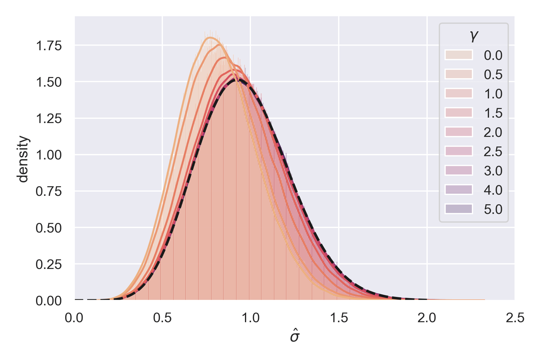
Figure 4: [Spiked tensor PCA, Section 5.2, example 4/4] The variance estimator is not distributed according to $\chi^{2}$-distribution with $\kappa=7$ degrees of freedom, it underestimates the variance. The dashed black line is the distribution of a $\chi(7)/\sqrt{7}$, and $\sigma=1$ in these experiments. The probability distribution function is estimated over $250,000$ Monte-Carlo samples for each value of $\gamma$.

Remark 5 (On the variance estimator).

The formula (4.5) involves the Student density function with $m-1$ degrees of freedom which necessitates several comments:

• First, this formula shows that ${\kappa}\,{\widehat{\sigma}^{2}}/{\sigma^{2}}$ (resp. $({m-1})\,{\widehat{\sigma}^{2}}/{\sigma^{2}}$) fails to be distributed according to a $\chi^{2}$-distribution with $\kappa$ (resp. $m-1$) degrees of freedom. This because $t_{1}$ is random.

• Second, Figure 4 illustrates that ${\widehat{\sigma}^{2}}$ under-estimates the variance $\sigma^{2}$ under the null ($\gamma=0$) or moderate alternatives ($\gamma\simeq 1$). The reason for this is clear: the chi-squared distribution assumes that the model is pre-specified, not chosen on the basis of $\sigma X(\cdot)$. But the Continuous LARS procedure has deliberately chosen the strongest predictor $\psi_{t_{1}}$, with $t_{1}\in M$ maximum of $Z(\cdot)$, among all of the available choices, so it is not surprising that it yields a drop in the value of the variance estimate on the residuals $Z^{|t_{1}}(\cdot)$.

• Third, Figure 4 shows that ${\kappa}\,{\widehat{\sigma}^{2}}/{\sigma^{2}}$ has almost $\chi^{2}$-distribution with $\kappa$ degrees of freedom for large alternatives ($\gamma=5$). The reason for this is clear: the mean $m(\cdot)$ is much larger than noise $\sigma X(\cdot)$ hence $t_{1}\simeq t_{0}$ and $\kappa\widehat{\sigma}^{2}/\sigma^{2}\simeq\kappa\widehat{\sigma}_{t_{1}}/\sigma^{2}$ which has $\chi^{2}$-distribution with $\kappa$ degrees of freedom.

5 Examples

5.1 How to deploy our method

We are given an observation $Y\in E$ as in Section 1.6 and we compute the corresponding profile likelihood random field given by $Z(t)=\langle Y,\Psi_{t}\rangle_{E}$. We would like to test the global nullity of its mean $m(\cdot)$ given by hypothesis (${\mathds{H}}_{0}$). The testing framework is depicted in Section 3.1 and we recall that

$$\Omega=\Lambda^{-\frac{1}{2}}_{2}(t_{1})\,(\nabla^{2}Z(t_{1})+\lambda_{1}\Lambda_{2}(t_{1}))\,\Lambda^{-\frac{1}{2}}_{2}(t_{1})\,.$$ (5.1)

The first and second maximum (and their arguments) are given by (2.8), which are computed using a Riemaniann gradient descent algorithm on $M$. We will give the expression of $\Lambda_{2}(t)$ in each example together with a closed form expression to compute the Riemaniann Hessian from the Euclidean Hessian and the Euclidean gradient. The Euclidean Hesssian can be computed using numerical differentiation or, in some cases, is given explicitly.

When the variance $\sigma^{2}$ is known, the testing statistics is given by Theorem 2. In particular, one needs to compute

$$G_{\Omega/\sigma}(\ell)=\int_{\ell}^{+\infty}\!\!\!\!\!\!\det(u\mathrm{Id}-\Omega/\sigma)\varphi(u)\,\mathrm{d}u\,.$$ (5.2)

When the variance $\sigma^{2}$ is unknown, the testing statistics is given by Theorem 3. In particular, one needs to compute

$$H_{{\Omega/\widehat{\sigma}}}(\ell)=\int_{\ell}^{+\infty}\!\!\!\!\!\det(u\operatorname{Id}-{\Omega/\widehat{\sigma}})\,f_{m-1}\Big{(}u\sqrt{({m-1})/{{\kappa}}}\Big{)}\,\mathrm{d}u\,,$$ (5.3)

where we recall that $f_{m-1}(\cdot)$ is the density of the Student $t$-distribution with $m-1$ degrees of freedom. Numerical integration can be done but, in some cases, we give explicit expressions of $G_{\Omega/\sigma}(\ell)$ and $H_{{\Omega/\widehat{\sigma}}}(\ell)$.

As for the variance estimation, we draw $\kappa$ independent points $(t_{d+2},\ldots,t_{m})$ uniformly on $M$. They generically satisfy Condition (${\mathrm{ND}(m)}$). For a putative point $t\in M$, the Gaussian vector $(X^{|t}(t_{d+2}),\ldots,X^{|t}(t_{m}))$ has for variance-covariance matrix $\sigma^{2}\Sigma$ where $\Sigma$ is some known matrix and an estimator of $\sigma^{2}$ is given by (4.1) with $t=t_{1}$ as in (4.4). In our experiments, we have drawn $5$ independent samples on $\kappa$ points and we found the same value for $\widehat{\sigma}$, as shown by the theory (4.3).

5.2 Spiked tensor PCA

We consider a simple example of the detection of a rank one $3$-way symmetric tensor observing $Y=\lambda_{0}t_{0}^{\otimes 3}+\sigma W$ where $W$ is an order $3$ symmetric tensor defined using symmetry and the following independent terms,

$$W_{iii} \text{ of variance }1;\text{ there are }3\text{ principal diagonal terms},i\in[3]\,,$$

$$W_{iij} \text{ of variance }1/3;\text{ there are }6\text{ sub-diagonals terms},i\neq j\in[3]\,,$$

$$W_{123} \text{ of variance }1/6;\text{ there is }1\text{ off-diagonal term}\,.$$

The profile likelihood is given by $Z(t)=\langle Y,t^{\otimes 3}\rangle_{E}=\lambda_{0}\langle t_{0},t\rangle^{3}+\sigma X(t)$ where $M=S^{2}$ is the $2$-sphere and $E$ is the Euclidean space of $3$-way symmetric tensors of size $3\times 3\times 3$ denoted by $(E,\langle\cdot,\cdot\rangle_{E})$ with dimension $m=10$. Hence, we have

$$\psi_{t} :=t^{\otimes 3}=(t_{i}t_{j}t_{k})_{1\leq i,j,k\leq 3}$$

$$c(s,t) :=\langle s,t\rangle^{3}$$

$$Z(t) :=\langle Y,\psi_{t}\rangle_{E}=\sum_{ijk}t_{i}t_{j}t_{k}Y_{ijk}$$

The reader may consult https://github.com/ydecastro/tensor-spacing/ for further details on the numerical experiments.

Hessian

To compute gradient and Hessian we can take advantage of the isometry of the problem and consider, without loss of generality, the case where $t\in M$ is the so-called “north pole”: $(0,0,1)$. We have

$$Z^{\prime}(0,0,1)=\left(\begin{array}[]{c}3Y_{133}\\ 3Y_{233}\\ 3Y_{333}\end{array}\right)\,.$$

This shows that $\Lambda_{2}=3\,\operatorname{Id}_{2}$ (on the tangent space), hence

$$\Omega=\sigma R(t_{1})=\frac{\sigma}{3}\widetilde{R}(t_{1})\,.$$

Since the second fundamental form of the unit sphere is $-\operatorname{Id}$, the Riemannian Hessian is equal to the Euclidean Hessian $Z^{\prime\prime}(t)$ limited to the tangent space $-\operatorname{Id}$ times the normal derivative (oriented outwards). The Euclidean Hessian $Z^{\prime\prime}(t)$ limited to the tangent space is given by

$$\left(\begin{array}[]{cc}2Y_{113}&Y_{123}\\ Y_{123}&2Y_{223}\end{array}\right)$$

This shows that the gradient is independent from the Hessian. To compute the independent part $R$ we can use

$$Z(0,0,1)=Z^{\prime}_{3}(0,0,1)=Y_{333}\quad\mbox{ and }\quad Z^{\prime}_{3}(0,0,1)=Y_{333}\,.$$

This shows that $R(t)$ is always equal to the Euclidean Hessian restricted to the tangent space. By (2.10), it yields

$$\Omega=\frac{\sigma}{3}\widetilde{R}(t_{1})=\frac{\sigma}{3}(\operatorname{Id}-\Pi_{t_{1}})\,Z^{\prime\prime}(t_{1})\,(\operatorname{Id}-\Pi_{t_{1}})\,,$$

where $\Pi_{t}:=tt^{\top}$ is the orthogonal projection onto the normal space at point $t$, and direct algebra gives

$$\frac{\partial^{2}Z}{\partial t^{i}\partial t^{j}}(t)=6\sum_{k=1}^{3}Y_{ijk}t^{k}\,.$$ (5.4)

Test statistics

One can compute the statistics $(t_{1},\lambda_{1})$ and $(t_{2},\lambda_{2})$ using a gradient descent. The expression of $\Omega$ has an explicit form by (5.4). Because we deal with $2\times 2$ matrices, we have for the spacing test the following identities,

$$G_{\Omega/\sigma}(\ell) =\int_{\ell}^{+\infty}\!\!\!\!\!\!\det(u\operatorname{Id}_{2}-\Omega/\sigma)\varphi(u)\,\mathrm{d}u$$

$$=\int_{\ell}^{+\infty}\!\!\!\!\!\!\big{[}(u^{2}-1)-\mathrm{Tr}(\Omega/\sigma)u+\det(\Omega/\sigma)+1\big{]}\varphi(u)\,\mathrm{d}u$$

$$=\ell\varphi(\ell)-\mathrm{Tr}(\Omega/\sigma)\varphi(\ell)+(\det(\Omega/\sigma)+1)(1-\Phi(\ell))\,,$$

with

$$\det(\Omega/\sigma) =(1/9\sigma^{2})\det\big{[}(\operatorname{Id}_{3}-\Pi_{t_{1}})Z^{\prime\prime}(t_{1})(\operatorname{Id}_{3}-\Pi_{t_{1}})+\Pi_{t_{1}}\big{]}$$

$$\mathrm{Tr}(\Omega/\sigma) =(1/3\sigma)\big{(}{\mathrm{Tr}(Z^{\prime\prime}(t_{1}))-t_{1}^{\top}Z^{\prime\prime}(t_{1})t_{1}}\big{)}\,.$$

As for the $t$-spacing test, one can check that

$$H {}_{\Omega/\widehat{\sigma}}(\ell)=\int_{\ell}^{+\infty}\!\!\!\!\!\!\det(u\operatorname{Id}_{2}-\Omega/\widehat{\sigma})\,f_{m-1}\Big{(}u\sqrt{({m-1})/{{\kappa}}}\Big{)}\,\mathrm{d}u$$

$$=\int_{\ell}^{+\infty}\!\!\!\!\!\!\big{[}u^{2}-\mathrm{Tr}(\Omega/\widehat{\sigma})u+\det(\Omega/\widehat{\sigma})\big{]}\,f_{m-1}\Big{(}u\sqrt{({m-1})/{{\kappa}}}\Big{)}\,\mathrm{d}u$$

$$=\frac{\kappa\sqrt{m-3}}{(m-2)\sqrt{m-1}}\frac{\Gamma(\frac{m}{2})\Gamma(\frac{m-3}{2})}{\Gamma(\frac{m-1}{2})\Gamma(\frac{m-2}{2})}\sqrt{\frac{\kappa}{m-3}}\bigg{[}\ell\sqrt{\frac{m-3}{\kappa}}f_{m-3}(\ell\sqrt{\frac{m-3}{\kappa}})+1-F_{m-3}(\ell\sqrt{\frac{m-3}{\kappa}})\bigg{]}$$

$$\quad-\mathrm{Tr}(\Omega/\widehat{\sigma})\frac{\kappa\sqrt{m-3}}{(m-2)\sqrt{m-1}}\frac{\Gamma(\frac{m}{2})\Gamma(\frac{m-3}{2})}{\Gamma(\frac{m-1}{2})\Gamma(\frac{m-2}{2})}f_{m-3}(\ell\sqrt{\frac{m-3}{\kappa}})$$

$$\quad+\det(\Omega/\widehat{\sigma})\sqrt{\frac{\kappa}{m-1}}\Big{(}1-F_{m-1}(\ell\sqrt{\frac{m-1}{\kappa}})\Big{)}\,,$$

with $m=10$, $\kappa=7$, $F_{\alpha}$ (resp. $f_{\alpha}$) the cumulative distribution function (resp. distribution density) of the Student $t$-distribution with $\alpha$ degrees of freedom and

$$\det(\Omega/\widehat{\sigma}) =(1/9\widehat{\sigma}^{2})\det\big{[}(\operatorname{Id}_{3}-\Pi_{t_{1}})Z^{\prime\prime}(t_{1})(\operatorname{Id}_{3}-\Pi_{t_{1}})+\Pi_{t_{1}}\big{]}$$

$$\mathrm{Tr}(\Omega/\widehat{\sigma}) =(1/3\widehat{\sigma})\big{(}{\mathrm{Tr}(Z^{\prime\prime}(t_{1}))-t_{1}^{\top}\sigma X^{\prime\prime}(t_{1})t_{1}}\big{)}\,.$$

The $t$-spacing test

In Figures 2 and 3, the alternative is given by $\lambda_{0}=\gamma\times\sigma\sqrt{3\log 3+3\log\log 3}$ where $\gamma=1$ corresponds to the so-called phase transition in Spiked tensor PCA as presented in Perry et al., (2020, Theorem 1.3). In Figure 3, the top right panel shows that $\lambda_{1}$ is stochastically increasing as $\gamma$ increases while the top right panel shows that the distribution of $\lambda_{2}$ remains unchanged for moderate values of $\gamma$, say $\gamma\geq 2$. It illustrates that the spacing between $\lambda_{1}$ and $\lambda_{2}$ grows linearly with $\gamma$. In the moderate regime, the bottom left panel shows that $\lambda_{1}$ is distributed as a Gaussian with mean $\lambda_{0}$ and variance $\sigma^{2}$ (dashed black line), which is the distribution of $Z(t_{0})$ under $\mathds{H}_{1}(t_{0},\lambda_{0})$. The bottom right panel shows that $t_{1}\simeq t_{0}$, for moderate values of $\gamma$. It illustrates that $(t_{1},\lambda_{1})$ is weakly close to the distribution of $(t_{0},Z(t_{0}))$, the ($t$-)spacing tests detect the alternative $\mathds{H}_{1}(t_{0},\lambda_{0})$.

5.3 Two-spiked tensor model

We consider a generalization to higher dimensions and two-spiked tensors of the preceding example (Section 5.2) by

$$Y=\nu_{0,1}x_{0}^{\otimes k}+\nu_{0,2}y_{0}^{\otimes k}+\sigma W\,,$$

where:

• the Euclidian space $E$ is given by $k$-way $n$-dimensional symmetric tensors ($k\geq 3,n\geq 4$) equipped with the dot product

  $$\forall\ \mathbf{T},\mathbf{U}\in({\mathds{R}}^{n})^{\otimes k}\,,\quad\langle\mathbf{T},\mathbf{U}\rangle_{E}=\sum_{i_{1},\ldots,i_{k}\in[n]}T_{i_{1},\ldots,i_{k}}U_{i_{1},\ldots,i_{k}}\,,$$ (5.5)

  with Euclidean or Frobenius norm $\|\mathbf{T}\|^{2}=\langle\mathbf{T},\mathbf{T}\rangle_{E}$, where $[n]=1,\ldots,n$;

• the noise tensor $W\in({\mathds{R}}^{n})^{\otimes k}$ is defined by

  $$W\>=\frac{1}{k!}\sum_{\pi\in{\mathfrak{S}}_{n}}G^{\pi}\,,$$ (5.6)

  where one considers i.i.d standard Gaussian $G_{i_{1}\cdots i_{k}}$ for indices ${1\leq i_{1},\ldots,i_{k}\leq n}$, ${\mathfrak{S}}_{n}$ is the set of permutations of the set $[n]$, and $G^{\pi}_{i_{1}\cdots i_{k}}=G_{\pi(i_{1})\cdots\pi(i_{k})}$. Note that the entries of $W$ with indices $i_{1}<i_{2}<\cdots<i_{k}$ form an i.i.d. collection of Gaussian random variables, namely $\{W_{i_{1}\cdots i_{k}}\}_{i_{1}<i_{2}<\cdots<i_{k}}$ with distribution $\mathcal{N}(0,1/(k!))$.

• the eigenvectors $x_{0}$ and $y_{0}$ are normalized and orthogonal, they belong to the Stiefel manifold ${\mathcal{M}}_{n,2}$ given by

  $${\mathcal{M}}_{n,2}:=\{(x,y)\in(S^{n-1})^{2}:x\perp y\}.$$

Using the framework of Section 1.3.2, we are led to consider the profile likelihood random field

$$t =(\theta,x,y)\in[0,2\pi)\times{\mathcal{M}}_{n,2}$$

$$\psi_{t} =\cos(\theta)x^{\otimes k}+\sin(\theta)y^{\otimes k}$$

$$Z(t) =\big{\langle}\psi_{t},Y\big{\rangle}_{E}=\cos(\theta)\langle x^{\otimes k},Y\rangle_{E}+\sin(\theta)\ \langle y^{\otimes k},Y\rangle_{E},$$

So the relevant manifold is $M=S^{1}\times{\mathcal{M}}_{n,2}$, where the circle $S^{1}$ is represented by $[0,2\pi)$. The dimension of $\mathrm{M}$ is $2n-2$. Hence we uncover

$$Y=\lambda_{0}\psi_{t_{0}}+\sigma W\,,$$

with $\lambda_{0}=\sqrt{\nu_{0,1}^{2}+\nu_{0,2}^{2}}$ and $\theta=\arccos\big{(}{\nu_{0,1}/\lambda_{0}}\big{)}$.

The covariance function at points $s=(\theta^{\prime},u,v)$ and $t=(\theta,x,y)$ is given by

$$c(s,t) =\operatorname{\mathds{E}}\big{(}Y(t)Y(s)\big{)}$$

$$=\cos(\theta)\cos(\theta^{\prime})\langle u^{\otimes k},x^{\otimes k}\rangle_{E}+\sin(\theta)\sin(\theta^{\prime})\langle v^{\otimes k},y^{\otimes k}\rangle_{E}$$

$$=\cos(\theta)\cos(\theta^{\prime})\langle u,x\rangle^{k}+\sin(\theta)\sin(\theta^{\prime})\langle v,y\rangle^{k}\,.$$ (5.7)

In particular, it follows that $c(t,t)=1$ for all $t\in{\mathrm{M}}$ and

$$c((\theta^{\prime},u,v),(\theta,x,y))=c((\theta^{\prime},Uu,Uv),(\theta,Ux,Uy)),$$ (5.8)

for any orthogonal map $U$ in $\mathds{R}^{n}$.

Let us compute the matrix $\Lambda_{2}(t)$.

Note that because of the partial invariance by isometry given by (5.8), $\Lambda_{2}(t)$ depends on $\theta$ only. Let us define for distinct $j\neq i,\ell\neq i$:

$$Y_{[i]} :=Y_{i,\ldots,i},\ \mbox{ with variance }1;$$

$$Y_{[i],j} :=Y_{i,\ldots,i,j}+\cdots+Y_{j,i,\ldots,i}=kY_{i,\ldots,i,j},\ \mbox{ with variance }k;$$

$$Y_{[i],j,\ell} :=\sum Y_{i_{1},i_{2},i_{3}}\mbox{ with }k-2\mbox{ occurences of }i,\mbox{ one }j\mbox{ and one }\ell,\ \mbox{ with variance }k(k-1);$$

$$Y_{[i],j,j} \mbox{ has variance }\frac{k(k-1)}{2}\,.$$

Because of the independence properties within $Y$, all these variables are independent. We consider the profile likelihood random field at point $(\theta,e_{1},e_{2})$ where $e_{1}$ and $e_{2}$ are the first two elements of the canonical basis. We have

$$Z(\theta,e_{1},e_{2})=\cos(\theta)Y_{[1]}+\sin(\theta)Y_{[2]}.$$

The Euclidean gradient at $(\theta,e_{1},e_{2})$ is given by

$$\frac{\partial Z(\theta,e_{1},e_{2})}{\partial x_{1}} =k\cos(\theta)Y_{[1]}, \frac{\partial Z(\theta,e_{1},e_{2})}{\partial y_{2}} =k\sin(\theta)Y_{[2]},$$

$$\frac{\partial Z(\theta,e_{1},e_{2})}{\partial x_{j}} =\cos(\theta)Y_{[1],j},j\neq 1, \frac{\partial Z(\theta,e_{1},e_{2})}{\partial x_{j}} =\sin(\theta)Y_{[2],j},j\neq 2\,,$$

and

$$\frac{\partial Z(\theta,e_{1},e_{2})}{\partial\theta}=-\sin(\theta)\ Y_{[1]}+\cos(\theta)Y_{[2]}\,.$$

Using the following orthonormal parameterization of the tangent space of the Stiefel manifold:

$$\left(\begin{array}[]{cc}0&\frac{-\Delta_{21}}{\sqrt{2}}\\ \frac{\Delta_{21}}{\sqrt{2}}&0\\ \Delta_{31}&\Delta_{32}\\ \vdots&\vdots\\ \Delta_{n1}&\Delta_{n2}\end{array}\right),$$

we get that the Riemannian gradient, including $\theta$, is given by

$$\nabla Z:=\left(\begin{array}[]{cc}\sin(\theta)Y_{[1]}+\cos(\theta)Y_{[2]}&\cdot\\ \frac{\cos(\theta)Y_{[1],2}-\sin(\theta)Y_{[2],1}}{\sqrt{2}}&\cdot\\ \cos(\theta)Y_{[1],3}&\sin(\theta)Y_{[2],3}\\ \vdots&\vdots\\ \cos(\theta)Y_{[1],n}&s\ Y_{[2],n}\end{array}\right)\,.$$ (5.9)

Hence, we deduce that

$$\Lambda_{2}(\theta)=\operatorname{diag}\big{(}1,k/2,\cos^{2}(\theta),\ldots,\sin^{2}(\theta),\ldots\big{)},$$ (5.10)

where the last two terms are repeated $n-2$ times.

Remark 6.

Observe that if $\theta=k\pi/2$ then the matrix $\Lambda_{2}(\theta)$ is singular. We prove in Lemma 8 of Appendix C that almost surely $\theta_{1}\neq k\pi/2$ where $t_{1}=(\theta_{1},x_{1},y_{1})$, hence $\Lambda_{2}(t_{1})$ is non-singular.

Also, Theorems 2 or 3 can not be directly applied. But, one can retrieve these results by omitting an $\varepsilon$-neighborhood of these points in the Kac-Rice formula and passing to the monotonic limit as $\varepsilon$ tends to $0$.

Let us compute the matrix $\Omega$.

Let us use for short $c$ and $s$ for $\cos(\theta)$ and $sin(\theta)$ respectively. We start by computing the Euclidian Hessian at $(\theta,e_{1},e_{2})$ as follows

$$\frac{\partial^{2}Z(\theta,e_{1},e_{2})}{\partial x^{2}_{1}} =ck(k-1)Y_{[1]}, \frac{\partial^{2}Z(\theta,e_{1},e_{2})}{\partial y_{j}\partial y_{j^{\prime}}} =s\ Y_{[2],j,j^{\prime}},j,j^{\prime}\neq 2,$$

$$\frac{\partial^{2}Z(\theta,e_{1},e_{2})}{\partial x_{1}\partial x_{j}} =c(k-1)Y_{[1],j},j\neq 1, \frac{\partial^{2}Z(\theta,e_{1},e_{2})}{\partial\theta\partial x_{1}} =ckY_{[1]},$$

$$\frac{\partial^{2}Z(\theta,e_{1},e_{2})}{\partial x_{j}\partial x_{j^{\prime}}} =cY_{[1]j,j^{\prime}},j,j^{\prime}\neq 1, \frac{\partial^{2}Z(\theta,e_{1},e_{2})}{\partial\theta\partial x_{j}} =ckY_{[1],j},j\neq 1,$$

$$\frac{\partial^{2}Z(\theta,e_{1},e_{2})}{\partial y_{2}^{2}} =s\ k(k-1)Y_{[2]}, \frac{\partial^{2}Z(\theta,e_{1},e_{2})}{\partial\theta\partial y_{2}} =s\ kY_{[2]},$$

$$\frac{\partial^{2}Z(\theta,e_{1},e_{2})}{\partial y_{j}\partial y_{j}^{\prime}} =s\ (k-1)Y_{[2],j},j\neq 2, \frac{\partial^{2}Z(\theta,e_{1},e_{2})}{\partial\theta\partial y_{j}} =s\ Y_{[2],j},j\neq 2,$$

and

$$\frac{\partial^{2}Z(\theta,e_{1},e_{2})}{\partial\theta^{2}}=-Z\,.$$

Note that all the cross derivatives between $x$ and $y$ vanish. The Riemannian Hessian consists of four parts (it can be checked by an order two Taylor expansion along the tangent space) namely

• The projected Euclidean Hessian: the Euclidean Hessian restricted to the tangent space;

• For each of the three vectors, $V_{1},V_{2},V_{3}$, normal to the Stiefel manifold, the part of the second fundamental form associated to the vector multiplied by the normal derivative.

The 3 components of the second fundamental form are

$$V_{1} =-\left(\begin{array}[]{ccc}1/2&0&0\\ 0&\operatorname{Id}_{n-2}&0\\ 0&0&0\end{array}\right)$$

$$V_{2} =-\left(\begin{array}[]{ccc}1/2&0&0\\ 0&0&0\\ 0&0&\operatorname{Id}_{n-2}\end{array}\right)$$

$$V_{3} =-\left(\begin{array}[]{ccc}0&0&0\\ 0&0&\frac{1}{\sqrt{2}}\operatorname{Id}_{n-2}\\ 0&\frac{1}{\sqrt{2}}\operatorname{Id}_{n-2}&0\end{array}\right)\,.$$

Hence, the expression of the Riemannian Hessian $\nabla^{2}Z(\theta,e_{1},e_{2})$ is

$$\left(\begin{array}[]{cccc}Z(\theta,e_{1},e_{2})&A&-s\big{(}Y_{[1],j}\big{)}_{j>2}&c\big{(}Y_{[2],j}\big{)}_{j>2}\\ \star&B&\frac{1}{\sqrt{2}}c\big{(}Y_{[1],2,j}\big{)}_{j}&-\frac{1}{\sqrt{2}}s\big{(}Y_{[2],1,j}\big{)}_{j}\\ \star&\star&c\big{(}(Y_{[1],j,j^{\prime}})_{j,j^{\prime}}-kY_{[1]}\operatorname{Id}_{n-2}\big{)}&-\big{(}cY_{[1],2}+sY_{[2],1}\big{)}\operatorname{Id}_{n-2}/2\\ \star&\star&\star&s\big{(}(Y_{[2],j,j^{\prime}})_{j,j^{\prime}}-kY_{[2]}\operatorname{Id}_{n-2}\big{)}\end{array}\right),$$

with $A=\frac{1}{\sqrt{2}}\big{(}cY_{[2],1}-sY_{[1],2}\big{)}$, and $B=-\frac{1}{2}\big{(}ckY_{[1]}+skY_{[2]}\big{)}+\frac{1}{2}\big{(}cY_{[1],2,2}+sY_{[2],1,1}\big{)}$.

To obtain $\nabla^{2}Z(t)$ for a generic point $(\theta,x,y)$ belonging to $\mathcal{M}_{n,2}$ we have to perform an isometry as in (5.8). Using (5.1), we deduce the expression of $\Omega$.

Testing procedures

The test statistics involve the function $G_{\Omega/\sigma}$ (resp. and $H_{\Omega/{\widehat{\sigma}}}$), recalled in Equation (5.2) (resp. and Equation (5.3)), which is given using an integral. This integration can be done numerically.

5.4 Super resolution

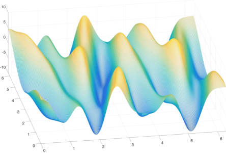
Figure 5: [Super-Resolution, Section 5.4] The super-resolution random field $Z(\cdot)$ depicts the observation of a point source at location $x_{0}$ on the interval $[0,2\pi)$ (spacial domain on the $x$-axis) with phase $\theta_{0}$ given on the $y$-axis. The $z$-axis corresponds to value of the profile likelihood $Z(x,\theta)$ at point $x$ with phase $\theta$.

In Signal processing, the super resolution phenomenon is the ability to distinguish two close sources (Dirac masses) from noisy low frequency measurements given by an optical system. This issue can be tackled using sparse regularization on the space of measures using the so-called Beurling-LASSO, introduced by De Castro and Gamboa, (2012); Azaïs et al., (2015); Candès and Fernandez-Granda, (2014); Duval and Peyré, (2015).

We consider the framework of Azaïs et al., (2020) where one observes $n=2f+1$ noisy frequencies between $-f$ and $f$ with $f\geq 1$. The $\ell^{th}$ Fourier coefficient of a point source (Dirac mass) at location $x_{0}$ with amplitude $\lambda_{0}$ and phase $\theta_{0}$ is $\lambda_{0}\,e^{\imath\theta_{0}}{e^{-\imath\ell x_{0}}}$. The observation is given by $Y=(y_{\ell})_{\ell}$ where $-f\leq\ell\leq f$, they are complex random variables given by

$$y_{\ell}=\lambda_{0}\,e^{\imath\theta_{0}}{e^{-\imath\ell x_{0}}}+\sigma W_{\ell}$$

with $\lambda_{0}>0$ the amplitude, $t_{0}=(x_{0},\theta_{0})\in[0,2\pi)^{2}$ the location and the phase of the source, and $\sigma>0$ the standard deviation of the noise. The noise is given by $W_{\ell}=\xi_{\ell,1}+\imath\xi_{\ell,2}$ with $\xi_{\ell,p}$ independent standard Gaussian variables, $-f\leq\ell\leq f$ and $p=1,2$.

The profile likelihood is given by

$$Z(t)=\langle Y,\psi_{t}\rangle_{E}=\lambda_{0}\cos(\theta-\theta_{0})\mathbf{D}_{f}(x-x_{0})+\sigma X(t)$$

with $t=(x,\theta)$, $M=[0,2\pi)^{2}$ is the $2$-Torus, $E=\mathds{C}^{n}$ equipped with the standard complex inner product, $X(\cdot)$ is a (real valued) centered Gaussian random field with covariance function $c(\cdot,\cdot)$, $\mathbf{D}_{f}$ is the Dirichlet kernel. The feature map, the Dirichlet kernel and the covariance function are given by

$$\psi_{t} =e^{\imath\theta}(e^{\imath fx},\ldots,e^{-\imath fx})\in\mathds{C}^{n}$$

$$c(t,t^{\prime}) =\cos(\theta-\theta^{\prime})\mathbf{D}_{f}(x-x^{\prime})\,,$$

$$\mathbf{D}_{f}(u) =\frac{\sin(fu/2)}{\sin(u/2)}\,,$$

An illustration of the super-resolution (profile likelihood) random field $Z(\cdot)$ is given in Figure 5. One can check that the assumptions of the present article are satisfied by the super-resolution random field. The spacing test is given by

$$\mathbf{S}_{\sigma}=\frac{\sigma(\alpha_{1}\lambda_{1}+\alpha_{2})\,\varphi(\lambda_{1}/\sigma)+(\alpha_{1}\sigma^{2}-\alpha_{3}^{2})\,(1-\Phi)(\lambda_{1}/\sigma)}{\sigma(\alpha_{1}\lambda_{2}+\alpha_{2})\,\varphi(\lambda_{2}/\sigma)+(\alpha_{1}\sigma^{2}-\alpha_{3}^{2})\,(1-\Phi)(\lambda_{2}/\sigma)}$$

where $\alpha_{1},\alpha_{2},\alpha_{3}$ have explicit forms given in (Azaïs et al.,, 2020, Proposition 10), $\lambda_{1}$ is the maximum of $Z(\cdot)$ and $\lambda_{2}$ the maximum of $Z^{|t_{1}}(\cdot)$. The $t$-spacing is explicitly described in Azaïs et al., (2020, Proposition 11).

5.5 Two-layers neural networks with smooth rectifier

Figure 6: a two-layers neural network with $c_{k}$ and $v_{i,j}$ real numbers.

We observe a $N$-sample $(x_{i},y_{i})_{i\in[N]}$, where $x_{i}\in\mathds{R}^{n}$ is the input and $y_{i}\in\mathds{R}$ the output. The output is such that $y_{i}=h(x_{i})+\sigma w_{i}$ for some measurable target function $h\,:\,\mathds{R}^{n}\to\mathds{R}$, standard deviation $\sigma>0$, and $w_{i}$ standard Gaussian variable.

We consider a two layer neural network given by

• (hidden layer) a layer of $r$ neurons with activation a $C^{2}$ function $\rho(\cdot)$;

• (output layer) and a layer which is simply a mean;

See Figure 6 for an illustration. As a consequence the output is $\frac{1}{r}\sum_{k=1}^{r}c_{k}\rho(\langle v_{k},x_{i}\rangle)$.

The unknown parameters are the weights $c_{k}$ and the directions $v_{k}$ of the neurons, for $k\in[r]$. We assume that $v_{k}\in\mathds{S}^{n-1}$. Using the trick that the mean of $r$ reals is the least squares estimator, we have to minimize

$$\frac{1}{N}\sum_{i=1}^{N}\Big{(}y_{i}-\frac{1}{r}\sum_{k=1}^{r}c_{k}\rho(\langle v_{k},x_{i}\rangle)\Big{)}^{2}=\frac{1}{Nr^{2}}\sum_{i=1}^{N}\sum_{k=1}^{r}\Big{(}y_{i}-c_{k}\rho(\langle v_{k},x_{i}\rangle)\Big{)}^{2}\,,$$

and we recognize the mean-square training error in the left hand side and the Euclidean distance between $Y=(y_{i})_{i,k}$ and $(c_{k}\rho(\langle v_{k},x_{i}\rangle))_{i,k}$ on the right hand side in $E=\mathds{R}^{N\times r}$ equipped with the dot product

$$\langle(a_{i,k}),(b_{i,k})\rangle_{E}=\frac{1}{N}\sum_{i=1}^{N}\Big{(}\frac{1}{r}\sum_{k=1}^{r}a_{i,k}\Big{)}\Big{(}\frac{1}{r}\sum_{k=1}^{r}b_{i,k}\Big{)}\,.$$

The Gaussian regression problem is $Y=H+\sigma W$ where $H=(h(x_{i}))_{i,k}$ and $W=(W_{i})_{i,k}$. To enter into the framework of Section 1.3.2 we need to perform the following change of variables

$$c_{k}\rho(\langle v_{k},x_{i}\rangle)=\lambda\frac{c_{k}V}{\lambda}\frac{\rho(\langle v_{k},x_{i}\rangle)}{V}=:\lambda a_{k}\frac{\rho(\langle v_{k},x_{i}\rangle)}{V},$$

with $V^{2}:=\sum_{i=1}^{N}\rho^{2}(\langle v_{k},x_{i}\rangle)$ and $\lambda^{2}:=V^{2}(c_{1}^{2}+\cdots+c_{r}^{2})$ are normalizing constants. One can check that $t=(a_{1},\dots,a_{r},v_{1},\dots,v_{r})\in S^{r-1}\times(S^{n-1})^{r}$ with $S^{r-1}$ the Euclidean sphere of ${\mathds{R}}^{r}$ and that ${\mathrm{M}}=S^{r-1}\times(S^{n-1})^{r}$. We have

$$\psi_{t}:=\Bigg{(}\frac{a_{k}\rho(\langle v_{k},x_{i}\rangle)}{\sqrt{\sum_{i^{\prime}}\rho^{2}(\langle v_{k},x_{i^{\prime}}\rangle)}}\Bigg{)}_{\begin{subarray}{c}k\in[r]\\ i\in[N]\end{subarray}}\text{ and }c(s,t):=\langle\psi_{s},\psi_{t}\rangle_{E}\,,$$

and the profile likelihood is $Z(t)=\langle H,\psi_{t}\rangle_{E}+\sigma X(t)$ with $X(t)=\langle W,\psi_{t}\rangle_{E}$ having covariance function $c(s,t)$.

Appendix of Second Maximum of a Gaussian Random Field and Exact ($t$-)Spacing test

In this appendix, the Riemannian Hessians are represented by $2$-forms.

Appendix A The helix random field

This section is a proof of Lemma 3. The argument is inspired from Azaïs and Wschebor, (2005, Lemma 4.1). Let $t\in{M}$ be a fixed point. On $L^{2}$, let $\Pi$ be the projector on the orthogonal complement to the subspace generated by $(X(t),\nabla X(t))$. Consider $h$ a vector of the tangent space at point $t$. Consider the exponential map $\varepsilon\mapsto\exp_{t}(\varepsilon h)$. This function is well defined on a neighborhood of $0$. Hence there exists $\varepsilon_{0}>0$ such that for all $\varepsilon\in]\varepsilon_{0},\varepsilon_{0}[$, the point $s(\varepsilon):=\exp_{t}(\varepsilon h)\in{M}$ exists. The function $\varepsilon\mapsto s(\varepsilon)$ is a parametrization of the geodesic starting at point $t$ with velocity $h$. We denote by $\varepsilon\mapsto h(\varepsilon)$ the parallel transport of $h$ along this geodesic. By Assumption ($\bf A_{1}$), the Taylor formula of order two gives

$$X(s(\varepsilon))=X(t)+\varepsilon\langle\nabla X(t),h\rangle+\frac{\varepsilon^{2}}{2}\nabla^{2}X(s(\varepsilon^{\prime}))[h(\varepsilon^{\prime}),h(\varepsilon^{\prime})]\,,$$ (A.1)

for some $\varepsilon^{\prime}\in[0,\varepsilon]$, and

$$c(s(\varepsilon),t)=1+\frac{\varepsilon^{2}}{2}\Lambda_{2}(t)[h,h]+o(\varepsilon^{2})\,,$$ (A.2)

by Assumption ($\bf A_{2}$). From (A.1), we have

$$\Pi(X(s(\varepsilon)))=\frac{\varepsilon^{2}}{2}\widetilde{R}(s(\varepsilon^{\prime}))[h(\varepsilon^{\prime}),h(\varepsilon^{\prime})]\,,$$

Note also that $-\Pi(X(s(\varepsilon)))$ is the numerator of $X^{|t}(s(\varepsilon))$ while the denominator is given by $-\frac{\varepsilon^{2}}{2}\Lambda_{2}(t)[h,h]+o(\varepsilon^{2})$ thanks to (A.2). We deduce that

$$X^{|t}(s(\varepsilon))=\frac{\widetilde{R}(s(\varepsilon^{\prime}))[h(\varepsilon^{\prime}),h(\varepsilon^{\prime})]}{\Lambda_{2}(t)[h,h]+o(1)}$$

From (2.6) and passing to the limit, we deduce that

$$\lim_{\varepsilon\to 0}X^{|t}(s(\varepsilon))=\frac{\widetilde{R}(t)[h,h]}{\Lambda_{2}(t)[h,h]}\,,$$

invoking that $\widetilde{R}$ is continuous by regression formulas and Assumption ($\bf A_{1}$), and that $\Lambda_{2}(t)[h,h]$ is positive by Assumption ($\bf A_{4}$).

For the second and last statement, observe that

$$\limsup_{s\to t}\,X^{|t}(s)\geq\sup_{\|h\|_{2}=1}\lim_{\varepsilon\to 0}X^{|t}(\exp_{t}(\varepsilon h))=\max_{\|h\|_{2}=1}\frac{\widetilde{R}(t)[h,h]}{\Lambda_{2}(t)[h,h]}=\frac{\widetilde{R}(t)[h_{0},h_{0}]}{\Lambda_{2}(t)[h_{0},h_{0}]}$$

where the vector $h_{0}$ exists by continuity of $h\mapsto{\widetilde{R}(t)[h,h]}/{\Lambda_{2}(t)[h,h]}$ on the Euclidean sphere, which is compact. Now, let $\delta>0$ and let $s_{n}$ be a sequence such that $s_{n}\to t$ and

$$\lim_{n\to\infty}\,X^{|t}(s_{n})\geq\limsup_{s\to t}\,X^{|t}(s)-\delta\,.$$

Note that the exponential map is a local diffeomorphism on a neighborhood of the point $t$. Hence, there exist a sequence of positive reals $\varepsilon_{n}$ converging to zero and a sequence $h_{n}$ of unit norm tangent vectors such that $s_{n}=\exp_{t}(\varepsilon_{n}h_{n})$. Since the Euclidean sphere is compact, we can extract a sequence such that $h_{n}$ converges to unit norm tangent vector $\overline{h}$. The Taylor formula gives that

$$X(s_{n}) =X(t)+\varepsilon_{n}\langle\nabla X(t),h_{n}\rangle+\frac{\varepsilon_{n}^{2}}{2}\nabla^{2}X(\widetilde{s}_{n})[\widetilde{h}_{n},\widetilde{h}_{n}]\,,$$

$$c(s_{n},t) =1+\frac{\varepsilon_{n}^{2}}{2}\Lambda_{2}(t)[h_{n},h_{n}]+o(\varepsilon_{n}^{2})\,,$$

for some $\widetilde{s}_{n}$ on the geodesic between $t$ and $s_{n}$ and $\widetilde{h}_{n}$ the parallel transport at point $\widetilde{s}_{n}$ of the tangent vector $h_{n}$ along this geodesic. By the $\Pi$-projection argument above, we deduce that

$$X^{|t}(s_{n})=\frac{\widetilde{R}(\widetilde{s}_{n})[\widetilde{h}_{n},\widetilde{h}_{n}]}{\Lambda_{2}(t)[h_{n},h_{n}]+o_{n}(1)}\,.$$

Passing to the limit by continuity yields

$$\max_{\|h\|_{2}=1}\frac{\widetilde{R}(t)[h,h]}{\Lambda_{2}(t)[h,h]}\geq\frac{\widetilde{R}(t)[\overline{h},\overline{h}]}{\Lambda_{2}(t)[\overline{h},\overline{h}]}=\lim_{n\to\infty}\,X^{|t}(s_{n})\geq\limsup_{s\to t}\,X^{|t}(s)-\delta\,.$$

Note that the most left hand side term does not depends on $\delta>0$, hence

$$\max_{\|h\|_{2}=1}\frac{\widetilde{R}(t)[h,h]}{\Lambda_{2}(t)[h,h]}\geq\limsup_{s\to t}\,X^{|t}(s)\,,$$

which concludes the proof.

Appendix B Ad-hoc Kac-Rice formula

The paper Azaïs and Wschebor, (2009, Theorem 7.2) concerns weighted sum of number of roots when the weight is a continuous function of time and of the level. This has been extended, by a monotone convergence argument to the case of lower semi-continuous weights in Armentano et al., (2023, Section 7)). However this is not sufficient mainly because the regularity of $\lambda_{2}^{t}$ as a function of $t$ is difficult to control. For this reason we must used the following tailored argument.

Denote by $\rm{dist}(s,t)$ the geodesic distance between points $s$ and $t$. Define

$$\forall t\in{M},\quad\lambda_{2,\epsilon}^{t}:=\sup_{s\in M\text{ s.t. }\mathrm{dist}(s,t)>\epsilon}\sigma X^{|t}(s)\quad\text{and}\quad\lambda_{2,\epsilon}:=\lambda_{2,\epsilon}^{{t_{1}}}\,,$$ (B.1)

and note that $\lambda_{2,\epsilon}^{t}$ is a continuous function of $t$. Define a monotone approximation $\xi_{n}(\cdot)$ of the indicator function ${\mathds{1}}\{\cdot\in B\}$. Then

$$\xi_{n}(\sigma X(t),\lambda_{2,1/n}^{t},\sigma R(t))\uparrow\mathds{1}\{(\sigma X(t),\lambda_{2}^{t},\sigma R(t)\in B\}\,.$$ (B.2)

So we can use Armentano et al., (2023, Section 7) for instance to compute the expectation of the left side of (B.2). Indeed, all conditions are clear except Condition c) of Armentano et al., (2023, Section 7) for $\lambda_{2,\epsilon}$ which is detailed hereunder. And then use monotone convergence theorem gives the result.

Checking Condition c) of Armentano et al., (2023, Section 7)

Using regression formulas, the distribution of $X(\cdot)$ under the condition $X(t_{0})=u$ admits the representation

$$X(t)=\widetilde{X}(t)+uf(t),$$

where $\widetilde{X}(t)$ corresponds to the distribution conditional to $X(t_{0})=0$. Our goal is to show the continuity of the distribution of $\lambda_{2}$ in this representation. The conditioned random field $\widetilde{X}(\cdot)$ satisfies

$$\forall\{s\neq t\}\,,\quad\rm{Cor}(X(s),X(t))<1\,.$$

so that, by the Tsirelson theorem, the maximum of $\widetilde{X}(\cdot)+uf(\cdot)$ is a.s. unique. The first consequence is the continuity, as a function of $u$, of $\widehat{t}$. For $t$ fixed, under $X(t_{0})=u$,

$$X^{|t}(s)=\widetilde{X}^{|t}(s)+ug^{|t}(s),\quad\rm{dist}(s,t)>\epsilon\,,$$

with obvious notation. The proof of Lemma 2 shows that $g^{|t}(s)$ is bounded uniformly in $s$ and $t$. This gives the desired continuity, as a function of $u$, of the distribution of $\lambda_{2,\epsilon}^{t}$ and then of $\lambda_{2,\epsilon}$.

Appendix C Two-spiked tensor profile likelihood

Lemma 8.

With probability $1$, it holds that $\theta_{1}\neq k\pi/2$.

Proof.

We prove that $\theta_{1}\neq 0$ a.s., the other cases are equivalent. Note that $\theta_{1}=0$ implies that there exists a point $x_{1}$ such that $f(x_{1})$ is the maximum of $f(x):=\langle x^{\otimes k},Y\rangle_{E}$ on $\mathds{S}^{n-1}$. As a consequence the gradient along $\mathds{S}^{n-1}$ is zero. Now, note that the derivative with respect to $\theta$ at $\theta=0$ of $Z(\theta,x_{1},y)$ is zero for every $y$ orthogonal to $x_{1}$. Choosing an orthonormal basis we obtain $n-1$ such derivatives.

Then, we use the Bulinskaya lemma (Azaïs and Wschebor,, 2009, Prop 6.11). We denote by $F(x),x\in\mathds{S}^{n-1}$ the random field defined on a set of dimension $n-1$ with values in $\mathds{R}^{2n-2}$ given by the $2n-2$ derivatives above. To use the Bulinskaya lemma we need to prove that

• the function $F(\cdot)$ has $\mathcal{C}^{1}$ paths,

• the density $p_{F(x)}$ is uniformly bounded.

Then since the dimension of the parameter set is smaller than the dimension of the image set, a.s there is no point $x$ such that $F(x)=u$ where $u$ is any value and in particular the value $0$.

Condition (i) is clear. To address Condition (ii), we can use the invariance by isometry and study the density $p_{F(x)}$ at the particular value $x=e_{1}$. We can consider the derivatives of $f(x)$ at $e_{1}$ along the basis of the tangent space $e_{2},\ldots,e_{n}$. We obtain $Y_{2[1]},\ldots,Y_{n[1]}$. Then we consider the derivatives in $\theta$ of $X(\theta,x_{1},y)$ with $y=e_{2},\ldots,e_{n}$ We obtain $Y_{[2]},\ldots,Y_{[n]}$. All these variables are independent with fixed variance so the density of $F(x)$ is bounded. ∎

References

- Adler and Taylor, (2009) Adler, R. J. and Taylor, J. E. (2009). Random fields and geometry. Springer Science & Business Media.
- Armentano et al., (2023) Armentano, D., Azaïs, J.-M., and León, J. R. (2023). On a general kac-rice formula for the measure of a level set. ArXiv preprint, abs/2304.07424.
- Auffinger and Ben Arous, (2013) Auffinger, A. and Ben Arous, G. (2013). Complexity of random smooth functions on the high-dimensional sphere. The Annals of Probability, 41(6):4214–4247.
- Azaïs et al., (2015) Azaïs, J.-M., De Castro, Y., and Gamboa, F. (2015). Spike detection from inaccurate samplings. Applied and Computational Harmonic Analysis, 38(2):177–195.
- Azaïs et al., (2017) Azaïs, J.-M., De Castro, Y., and Mourareau, S. (2017). A rice method proof of the null-space property over the grassmannian. In Annales de l’Institut Henri Poincaré (B) Probabilités et Statistiques.
- Azaïs et al., (2020) Azaïs, J.-M., De Castro, Y., and Mourareau, S. (2020). Testing gaussian process with applications to super-resolution. Applied and Computational Harmonic Analysis, 48(1):445–481.
- Azaïs and Wschebor, (2004) Azaïs, J.-M. and Wschebor, M. (2004). Upper and lower bounds for the tails of the distribution of the condition number of a gaussian matrix. SIAM Journal on Matrix Analysis and Applications, 26(2):426–440.
- Azaïs and Wschebor, (2005) Azaïs, J.-M. and Wschebor, M. (2005). On the distribution of the maximum of a gaussian field with d parameters. The Annals of Applied Probability, 15(1A):254–278.
- Azaïs and Wschebor, (2009) Azaïs, J.-M. and Wschebor, M. (2009). Level sets and extrema of random processes and fields. John Wiley & Sons Inc.
- Candès and Fernandez-Granda, (2014) Candès, E. J. and Fernandez-Granda, C. (2014). Towards a mathematical theory of super-resolution. Communications on pure and applied Mathematics, 67(6):906–956.
- Chizat, (2022) Chizat, L. (2022). Sparse optimization on measures with over-parameterized gradient descent. Mathematical Programming, 194(1):487–532.
- De Castro et al., (2021) De Castro, Y., Gadat, S., Marteau, C., and Maugis-Rabusseau, C. (2021). Supermix: sparse regularization for mixtures. The Annals of Statistics, 49(3):1779–1809.
- De Castro and Gamboa, (2012) De Castro, Y. and Gamboa, F. (2012). Exact reconstruction using beurling minimal extrapolation. Journal of Mathematical Analysis and applications, 395(1):336–354.
- Duval and Peyré, (2015) Duval, V. and Peyré, G. (2015). Exact support recovery for sparse spikes deconvolution. Foundations of Computational Mathematics, 15(5):1315–1355.
- Efron et al., (2004) Efron, B., Hastie, T., Johnstone, I., Tibshirani, R., et al. (2004). Least angle regression. The Annals of statistics, 32(2):407–499.
- Lifshits, (1983) Lifshits, M. A. (1983). On the absolute continuity of distributions of functionals of random processes. Theory of Probability & Its Applications, 27(3):600–607.
- Perry et al., (2020) Perry, A., Wein, A. S., and Bandeira, A. S. (2020). Statistical limits of spiked tensor models. Annales de l’Institut Henri Poincaré, Probabilités et Statistiques, 56(1):230 – 264.
- Steinwart and Christmann, (2008) Steinwart, I. and Christmann, A. (2008). Support vector machines. Springer Science & Business Media.