11email: bmm@cab.inta-csic.es
Surface parameterisation and spectral synthesis
of rapidly rotating stars††thanks: The codes and all the files required to carry out the computations
described in this paper are available at
https://github.com/astrobmm/fastrot-spec
Abstract
Context. Spectral synthesis is a powerful tool with which to find the fundamental parameters of stars. Models are usually restricted to single values of temperature and gravity, and assume spherical symmetry. This approximation breaks down for rapidly rotating stars.
Aims. This paper presents a joint formalism to allow a computation of the stellar structure — namely, the photospheric radius, , the effective temperature, , and gravity, — as a function of the colatitude, , for rapid rotators with radiative envelopes, and a subsequent method to build the corresponding synthetic spectrum.
Methods. The structure of the star is computed using a semi-analytical approach, which is easy to implement from a computational point of view and which reproduces very accurately the results of much more complex codes. Once , , and are computed, the suite of codes, atlas and synthe, by R. Kurucz are used to synthesise spectra for a mesh of cells in which the star is divided. The appropriate limb-darkening coefficients are also computed, and the final output spectrum is built for a given inclination of the rotation axis with respect to the line of sight. All the geometrical transformations required are described in detail.
Results. The combined formalism has been applied to Vega, a rapidly rotating star almost seen pole-on, as a testbed. The structure reproduces the results from interferometric studies and the synthetic spectrum matches the peculiar shape of the spectral lines well.
Conclusions. Contexts where this formalism can be applied are outlined in the final sections.
Key Words.:
stars: rotation – stars: structure – stars: spectra1 Introduction
Spectral synthesis is one of the most powerful techniques to characterise a star. Comparing the high-resolution spectra of a given target with synthetic models usually provides very accurate stellar parameters. The spectroscopic analysis must be complemented with a detailed analysis of the spectral energy distribution, built from photometric observations, and, when feasible, with the use of astrometric and interferometric observations.
A vast amount of work has been done in the field of spectral synthesis: an extensive list of the main 1D-LTE codes available can be found in the introduction of the paper by Wheeler et al. (2023). All these codes allow us to compute spectra for a given set of parameters; in particular, single values of the effective temperature, , and gravity, (other inputs, such as metallicity, [M/H], and microturbulence are also required). In some cases — for example, synthe (Kurucz, 2014), the codes can be adapted to simulate the spectrum of a rotating star by computing individual surface intensities at different inclinations through the atmosphere, applying the appropriate Doppler shifts, corresponding to the projected rotation speed, , to the emergent spectra.
Single values of and in modelling a stellar spectrum imply the underlying limitation of spherical symmetry. This approximation breaks down for rapidly rotating stars:111To give an idea of what ‘rapidly rotating’ means, and in anticipation of results that can be obtained with the models presented in this paper, for a star with =2.0, =2.5, =9000 K, and =120 km s-1, one obtains and K; these values are significant enough to assess the need of considering the oblateness of the star in this context. in that regime, the star becomes oblate, and all the relevant photospheric variables, in particular the radius, temperature and gravity, become functions of the latitude, making the problem complex both from the theoretical and computational points of view. Examples of the departure from spherical symmetry are the results of the works — all based on interferometric observations — by Bouchaud et al. (2020) on Altair ( aql, A7V), who find that ; Domiciano de Souza et al. (2014) on Achernar ( Eri, B6Vpe), giving a ratio ; and Monnier et al. (2012), on Vega ( Lyr, A0V), for which (Model 3 of that paper).
In consequence, the first issue to be tackled before proceeding to the computation of a synthetic spectrum for a rotating star is that of its structure; in particular, finding out the dependence of , , and with latitude; the effective gravity, , is defined as the vector sum of the classical gravity and the centrifugal acceleration (see Eqn. 4 in Sect. 3). This area of research has a long history, whose starting point can be set in the pioneering works by von Zeipel (1924a, b), who found that in barotropic stars the energy flux is proportional to the local effective gravity, leading to , with . This is the well-known so-called von Zeipel law, which was modified by Lucy (1967), proposing a smooth dependence, , for stars with a convective envelope. is traditionally called the ‘gravity-darkening exponent’, the term ‘gravity darkening’ encompassing all the phenomena involved when the rotation of the star is considered — polar temperature and gravity larger than the equatorial values, polar radius shorter than the equatorial radius — is the common terminology today. Espinosa Lara & Rieutord (2012) discussed the relevance of gravity darkening and warned about the caveats posed by the dependence of the resulting laws on the stellar atmosphere models chosen.
The review by Rieutord (2006) gives a summary of the advances in modelling rapidly rotating stars in the decades preceding that paper. In recent years, substantial progress has been made. In particular, concerning the work in this paper, we mention ESTER (Evolution STEllaire en Rotation, Espinosa Lara & Rieutord, 2013; Rieutord et al., 2016, and references therein). ESTER is the first code computing, in a consistent way, 2D models of fast-rotating stars, including their large-scale flows. A semi-analytical approximation of this code is used in this work.
The main goal of this paper is to provide a set of methods, described in as much detail as possible, to carry out from scratch the structure and computation of the synthetic spectrum for a rotating star. To our knowledge, there is no publicly available code to carry out these combined tasks. In particular, the prescription presented here for computing the stellar structure has the advantage of being valid for any rotation and is not restricted to slow rotators, in contrast with the von Zeipel approximation (see Sect. 3). A good example of the utility of these tools is the work by Lazzarotto et al. (2023), in which the authors combine the use of synthetic spectra and the ESTER model to carry out a photometric determination of the inclination, rotation rate, and mass of rapidly rotating intermediate-mass stars.
The paper is organised as follows: In Sect. 2, we describe how a star with an inclination angle, , with respect to the line of sight is seen by the observer, and how to carry out the projection onto a 2D plane. In Sect. 3, we describe how to obtain the relevant parameters for a rotating star required to carry out the spectral synthesis. In Sect. 4, we describe how to build the synthetic spectrum of a star where , , and are functions of the latitude. In Sect. 5, we apply the whole formalism to Vega as a testbed. Sections 6 and 7 include a discussion of the results and some conclusions. Since this paper deals with formalisms of different areas of stellar physics — namely, geometry, structure, spectral synthesis, and limb darkening — we give in each section the basic information and equations, and direct the reader to the appropriate references.
2 The geometry
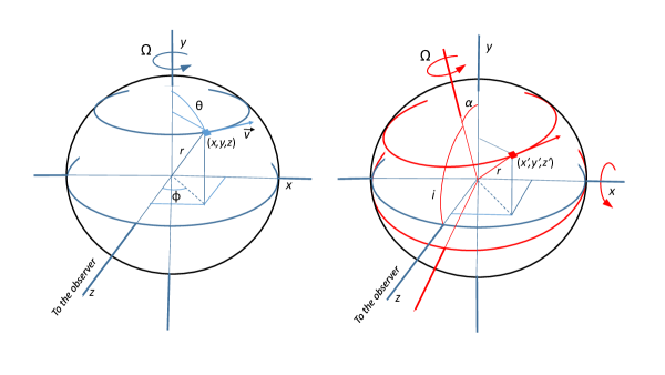
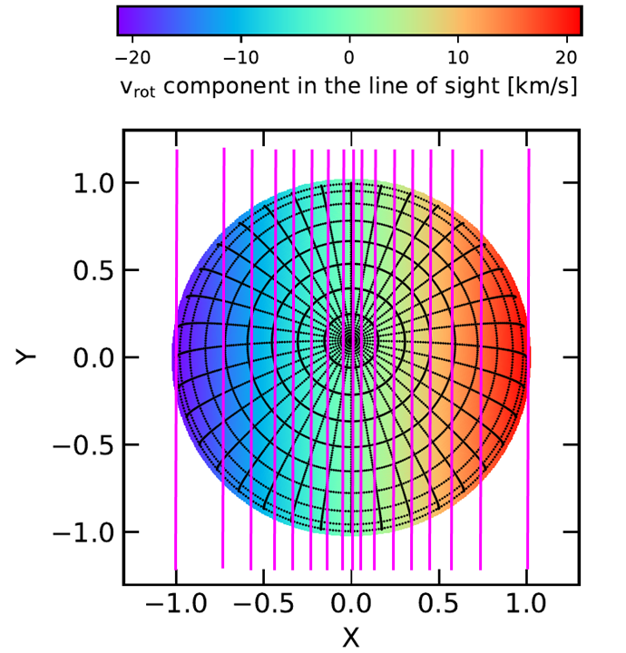
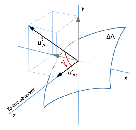
Figure 1 shows the geometry that is used throughout the paper. Initially, all the calculations are done considering that the rotation axis is perpendicular to the line of sight, which coincides with the axis (left). The star is then inclined by an angle of around the axis, where is the inclination (, pole-on, , equator-on) (right). Polar coordinates are used, where is the colatitude (0 for latitude , for latitude ), and the azimuthal angle. Since the stellar rotation takes place around the axis, all variables are only functions of colatitude, and are symmetric with respect to the equator.
In Appendix A, all the details concerning the projection of the 3D star onto the 2D plane of the sky, and how some quantities are seen from the point of view of the observer, are given. Information on how to compute all the relevant geometrical variables that arise when dealing with an oblate star is also provided.
3 Parameterisation of the stellar surface
In this work, we follow the model of Espinosa Lara & Rieutord (2011) (ER11, hereafter), also called ’-model’. A very detailed discussion of its derivation can be found in the work of Rieutord (2016). Their starting point is the fact that the gravity darkening of rapidly rotating stars is not well described by the von Zeipel (1924a) law, parameterised, as we mentioned before, as , where and are the effective temperature and effective gravity, respectively. Their work was triggered by the fact that some interferometric works (see references in ER11) showed that von Zeipel’s approach seems to overestimate the temperature difference between the pole and the equator of the star. The formalism presented in ER11 allows the computation of , , and of the photosphere of a rotating star, improving the results obtained following von Zeipel’s prescription. Although simple, mainly from a computational point of view, the ER11 model is able to reproduce the results of more complex models; in particular, the above-mentioned ESTER, as can be seen in Fig. 2 of ER11. The model is tailored for stars with radiative envelopes.
The two basic equations of the model are
| (1) |
, that is, the Roche model (see ER11), and
| (2) |
where
| (3) |
is the non-dimensional rotation rate, , , and are the angular velocity, the Keplerian angular velocity, and the radius, respectively, the last two at the equator, , is the non-dimensional radial coordinate, and , as we mentioned, is the colatitude. is an auxiliar angular variable (see ER11 for details, also concerning the two singularities in Eq. (2) at and ).
Equation (1) provides the values of the photospheric radius, , as a function of ; then for each colatitude, is introduced into Eq. (2) to obtain . Both equations can be solved by bisection, or by a Newton-Raphson method. Once these two variables, ) and are computed, the effective gravity and the effective temperature can be obtained from the following expressions:
| (4) |
| (5) |
We note that Eqs. (4) and (5) include three quantities, namely, the stellar mass and luminosity, and the equatorial radius, which — in particular and — are not usually known with an acceptable degree of accuracy. Even the luminosity, , is a more subtle parameter to estimate in the case of very flattened stars since the same object, seen pole-on or equator-on, would show to the observer different spectral energy distributions, which would lead to different apparent effective temperatures, and hence luminosities, the reason being that the expression loses its meaning since both temperature and radius are functions of the latitude.
In a practical case, when attempting to model a stellar spectrum by building a grid of models, a reasonable range of masses, consistent with the estimated spectral type of the object, can be used in Eq. (4). As for the luminosity and equatorial radius, the first parenthesis of the second expression of Eq. (5), including the exponent 1/4, is basically the equatorial effective temperature, and therefore can be substituted by an estimation of , or alternatively of the polar temperature, , using Eq. (32) of ER11:
| (6) |
building the grid using as inputs a range of values of or that are also consistent with an initial estimate of the spectral type, and iterating until both the interferometric results are reproduced, and/or the synthetic spectrum matches the observed one. In the most common situation, in which interferometric observations are not available, the peculiar shape of some spectral lines (see Sect. 5) can give hints about the inclination of the star, and together with an estimate of the projected rotation speed, , iterate using a range of temperatures, until an agreement between the observations and the model is reached.
We note that, according to the first expression in Eq. (5), von Zeipel’s law, , is recovered for slow rotations since as decreases, (see Eq. (2)). As a final remark, we also note that in previous works modelling interferometric data (Aufdenberg et al., 2006; Monnier et al., 2012) the methods involving the calculation of the stellar radius, temperature, and gravity make explicit use of the gravity-darkening law , whereas the ER11 formalism used in this work allows us to avoid the whole discussion of what the appropriate value of the exponent, , is.
4 Spectral synthesis
The spectral synthesis of a star whose relevant photospheric variables are functions of the latitude is, from a computational point of view, substantially more difficult than the classical single-temperature, single-gravity modelling; however, it is conceptually fairly intuitive and can be carried out by following these steps:
-
1.
Once the structure is computed according to the prescription described in Sect. 3, the star is divided into cells delimited by the intersection of a mesh of parallels and meridians with separations of ; that implies cells, of which half are visible to the observer. We point out that this discretisation of the stellar surface is uneven, in the sense that the areas of cells near the polar regions are smaller than those of cells near the equator. A discretisation keeping the surface area of all cells constant (see e.g. Bouchaud et al., 2020; Lazzarotto et al., 2023) leads to exactly the same results as the ones presented in this work. A finer mesh does not result in any improvement or refinement of the output spectrum. No numerical noise appears in the results from any of the discretisations.
-
2.
Since all variables, in particular and , are only functions of latitude, 90 synthetic spectra, corresponding to the cells with colatitudes between 0 and , are computed for the corresponding values of temperature and gravity. The angular speed, metallicity, and microturbulence are fixed. These synthetic spectra, which contain the fluxes in erg cm2 s-1 Å-1, are not rotationally broadened.
-
3.
After the star is rotated by an angle, , around the axis, each individual cell is seen by the observer with a projected area, , a radial velocity, , and an angle, , between the line of sight and the normal to the surface element, the latter being relevant for the correction for limb darkening, , to be applied (see Appendix B for details of the computation of the limb-darkening coefficients). Taking into account all these factors, the total flux at a given wavelength, , is
(7)
The individual synthetic spectra are computed using the codes atlas and synthe (Kurucz, 2014) and the models containing the elemental abundances and the stratification of the stellar atmospheres as a function of temperature, gravity, metallicity, and microturbulence velocity (Castelli & Kurucz, 2003). The atlas code allows us to compute a model atmosphere for any value of temperature and gravity from a close model already computed in the Castelli & Kurucz grids. The spectral synthesis is carried out using synthe, with a resolution of at 450 nm (0.0045 nm/pixel). The GNU-linux version of the codes by Sbordone (2005) is used.222The codes, models, and further information can be found at the URL: https://wwwuser.oats.inaf.it/fiorella.castelli/
A grid of 3668 synthetic models with between 7000 and 20000 K (step 100 K), =3.0, 3.5, 4.0, 4.5, and metallicities of [M/H]=, , , , , 0.0, and was computed beforehand; the microturbulent velocity is 2 km s-1. For all the cells at a colatitude, , with parameters , the corresponding synthetic spectrum is computed by linear interpolation between the four closest neighbouring models in the grid, those bracketing at a time the temperature and the gravity of the cell; that is, the four models in the grid — for a given metallicity — , , , and , have to fulfil , .
The interpolation is easily carried out in this way: first, two constants are defined as
| (8) |
then two intermediate models are computed, which are combined to give the final one for the -th cell:
| (9) |
5 Vega as a testbed
Vega ( Lyr, HD 172167, HIP 91262, HR 7001) is one of the most extensively studied stars. It is well known that it is used as standard for the calibration of several photometric systems (Bessell, 2005) and that it is surrounded by a debris disc, discovered by Aumann et al. (1984), which triggered an intensive study at infrared wavelengths (Sibthorpe et al. 2010, and references therein). However, this object turned out not to be the perfect standard, showing anomalies in its luminosity (Petrie, 1964; Millward & Walker, 1985), some peculiarly shaped absorption lines (Gulliver et al., 1991), and its radius (Hanbury Brown et al., 1967; Ciardi et al., 2001) in comparison with other A0 V stars.
Concerning this paper, our interest focuses on the fact that all these anomalies are now explained by the fact that Vega is a rapidly rotating star being seen almost pole-on; that is, with a small inclination angle, as has been shown by a number of interferometric studies (Aufdenberg et al., 2006; Peterson et al., 2006; Monnier et al., 2012) and spectroscopic analyses (Gulliver et al., 1991; Hill et al., 2004; Takeda et al., 2008; Yoon et al., 2010; Hill et al., 2010; Takeda, 2021). Table 1 in Takeda (2021) gives a summary of the values of the projected equatorial velocity, , the equatorial velocity, , the inclination angle, , the polar and equatorial radii, and , and the rotation period, , according to different analyses.
To check the reliability of the methods described in this paper, we use some of the results of the above-mentioned works to check whether the structural model (Sect. 5.1), and then the spectral synthesis model (Sect. 5.2), can reproduce the observed properties.
| Input parameters | |
|---|---|
| Inclination, (degrees) | 6.2a |
| Stellar mass, | 2.15a |
| Polar temperature, (K) | 10000 |
| Equatorial radius, | 2.726a |
| Normalised , | 0.510 |
| Metallicity, [M/H] | |
| Derived parameters | |||
|---|---|---|---|
| This work | Other works | ||
| 2.412 | 2.4180.012a | ||
| 1.130 | 1.127a | ||
| (K) | 8902 | 8910130a | |
| 46.5 | 47.22.0a | ||
| 0.890 | 0.885a | ||
| 3.769 | |||
| 4.005 | |||
| (km s-1) | 197.8 | 19515b | |
| (km s-1) | 21.4 | 21.60.3b | |
| Averaged (K) | 9430 | 936090a | |
| Averaged | 3.958 | ||
| Stellar surface area | 11.536† | ||
| Refs.: (a) Monnier et al. (2012), (b) Takeda (2021). | |||
| (): In units of . A sphere with would have | |||
| a surface area . | |||
5.1 Structure and stellar parameters
Table 1 shows in the upper part the input parameters of the model; the inclination, stellar mass, and equatorial radius have been taken from Monnier et al. (2012) (their Model 3, the ‘concordance model’). Since the model also requires the polar temperature and as inputs, was explored within the uncertainty interval given by Monnier et al. to match the luminosity, and was fixed to match the value of derived by Takeda (2008). The lower part of the table (Col. 2) shows the results of the formalisms described in Sects. 2 and 3; Col. 3 shows, for comparison, some parameters derived from interferometric (Model 3 by Monnier et al., 2012) and spectroscopic analyses (Takeda, 2021).
The results derived in this work are in general consistent with those from previous modellings, although some discrepancies are apparent: the temperature drop from pole to equator, 1098 K in our case, is in agreement with that by Monnier et al. (2012) (1160 K); both are substantially smaller than those by Peterson et al. (2006) ( K), and Aufdenberg et al. (2006) (2250 K).
Some details about the calculations: the stellar luminosity was computed by adding for all cells the quantity , where and are the surface area and the effective temperature of the -th cell; and the average effective temperature was estimated from the expression , where is an average of the radius, computed in the interval of colatitudes, .
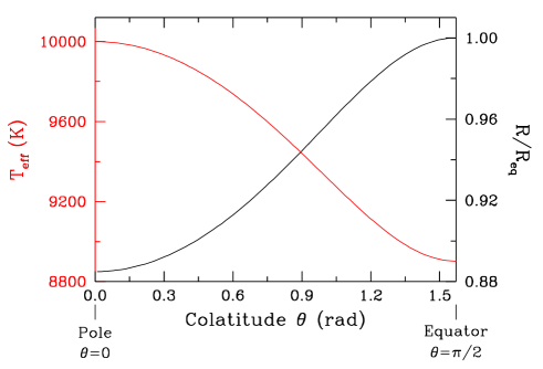
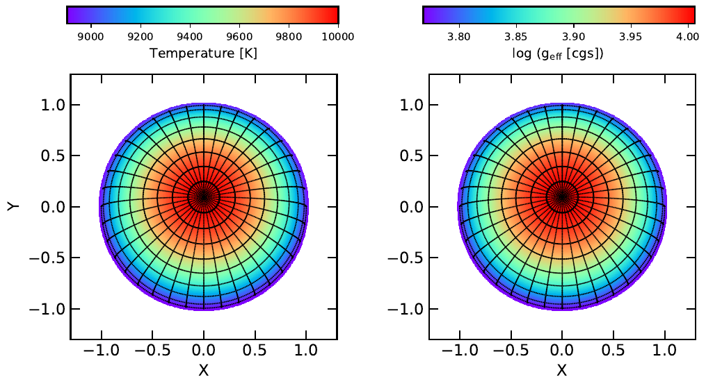
Figure 2 shows the stellar radius normalised to (black) and the temperature (red), plotted against the colatitude for the northern hemisphere (the results for the southern hemisphere are symmetrical). Fig. 3 shows two colour plots showing the temperature and effective gravity profiles for Vega according to the results of our modelling.
5.2 Spectral synthesis
In this section, we check whether the results derived in Sect. 5.1 together with the formalism described in Sect. 4 are able to reproduce the peculiar shape of some features of the spectrum of Vega. The high-resolution, high-signal-to-noise spectrum atlas of Vega from Takeda et al. (2007) has been used throughout. We do not intend here to make an analysis of the elemental abundances, which has already been carried out by other authors (see e.g. Ilijic et al., 1998; Qiu et al., 2001; Takeda, 2008; Takeda et al., 2008), but rather to make sure that the whole set of procedures described in the previous sections is able to reproduce the peculiar shapes of the absorption lines of the spectrum of Vega.
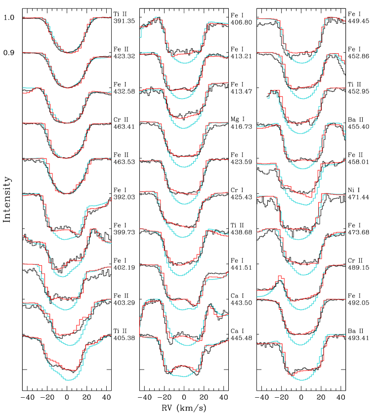
Figure 4 shows the profiles of 30 lines, from different species, both neutral and ionised. The observed profiles and the results of our modelling are plotted in black and red, respectively. In cyan, the profiles resulting from a single-temperature, single-gravity synthetic spectrum computed with the average parameters, and , listed in Table 1, are also plotted. For the sake of a better graphical display of the whole set of lines, both the observed and the synthetic profiles have been re-scaled and normalised, placing the continuum at intensity 1.0 and the bottom of the profiles at intensity 0.9, whereas the single-temperature, single-gravity profiles have been scaled so that they fit the wings of the observed absorptions.
The first five profiles of the left panel, from top to bottom, show rounded shapes, typical of lines broadened with a classical rotation profile; however, the remaining 25 profiles have a variety of shapes, the most extreme cases being those that are almost rectangular, such as Fe i 402.19, 406.80, 449.45 nm and Ba ii 455.40, 493.41 nm, or those showing two deeper components at velocities close to , like Ca i 445.48 nm. It is apparent that in all cases the agreement between the shape of the observed profiles and the results from the formalism described in Sect. 4 is remarkable. To our knowledge, the only work that also accurately reproduces the peculiar profiles of the Vega spectrum is that from Takeda et al. (2008).
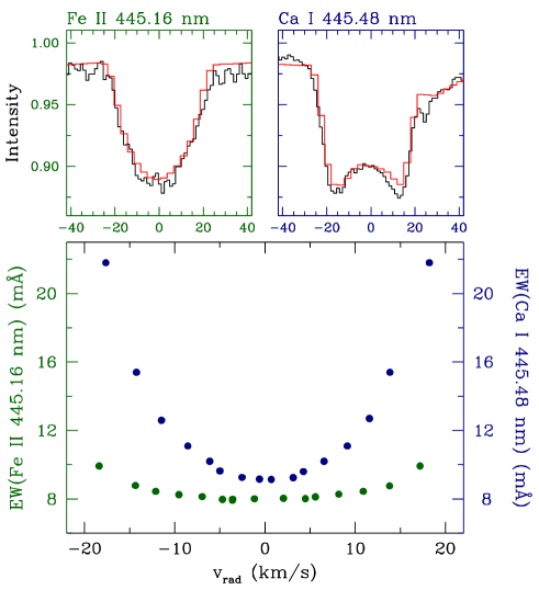
In order to understand the peculiar profile of some lines, we show as an example an analysis of two nearby lines; namely, Fe ii 445.16 nm, which has a rounded shape, and the above-mentioned Ca i 445.48 nm. The left panel of Fig. 5 shows the colour plot of the radial velocity of each surface element for the Vega model. It is well known that the loci of equal radial velocities, in the case of solid-body rotation, as seen by an observer, are lines parallel to the rotation axis projection; that is, all points in the disc with =constant (see e.g. Gray, 1992, chapter 18) have the same value of radial velocity. Since the star is seen almost pole-on, the regions close to the borders of the disc — the limb, which coincides with the equator — and in particular those with the highest projected rotation speeds, are the ones with the lowest temperatures and gravities. Therefore, the ionisation balance of some species differs from regions with low temperatures and gravities to regions near the pole (see Fig. 3). The vertical purple lines superimposed on the colour plot of the star in the left panel of Fig. 5 delimit 16 strips. Their widths have been computed to fulfil the condition that each one contributes to the full synthetic spectrum with the same amount of flux in the continuum near the lines.
The right panel of Fig. 5 shows the stellar lines (black), with the corresponding model profiles (red) framed in green (Fe ii) and blue (Ca i) boxes, respectively, and the equivalent widths (EWs) of the contributions to the profiles from each one of the 16 strips, using the same colour code. The different ranges of EWs for both lines are apparent: whereas the values for the Fe ii values are more even, leading to a rounded profile, the outer strips dominate the absorption of the Ca i line, producing its peculiar shape.
6 Discussion
6.1 The -model versus the von Zeipel approach
Despite the fact that the -model, and the corresponding spectral synthesis, work well for Vega, it is interesting to point out that Takeda (2008), using the Roche model and the von Zeipel value of the gravity darkening exponent, , also found a good agreement between modelling and observations. Monnier et al. (2012) showed that the value of that best fit the observations was , in agreement with the von Zeipel value; therefore, both the -model and the von Zeipel approximation give accurate results for Vega.
To show the real potential of the -model, it is interesting to explore the case of a much faster rotator for which the exponent is much less then 0.25. The case of Achernar is a good one to check, since a value of must be used to reproduce the observed results (Domiciano de Souza et al., 2014). The -model, using as inputs — all extracted from Domiciano de Souza et al.’s paper — , K, , and , gives K, in excellent agreement with the best fit of the CHARRON RVZ model to the VLTI/PIONIER H band observations, which gives K. In contrast, the von Zeipel model () gives K, almost 1800 K off the value derived from observations, which is nicely reproduced by the -model (see Domiciano de Souza et al., 2014, for further details). Obviously, that deviation would have a large impact on reproducing the observed spectrum, via spectral synthesis.
6.2 Contexts in which this work can be useful
Once the whole formalism of the -model plus the spectral synthesis have been put together and successfully tested with the paradigmatic case of Vega, and the reassuring case of Achernar mentioned in the previous subsection, it is interesting to point out explicitly in which contexts all this can be useful. With this purpose, we have computed several models whose details are given in Table 2. The models share as fixed inputs some of the parameters of the structural model of Vega (see Table 1); namely, the stellar mass, polar temperature, equatorial radius, and metallicity. Models in the upper half of Table 2 have been computed with a fixed inclination, , the value obtained for Vega, and five values of , resulting in five values of ; namely 10, 15, 20, 21.4 (Vega), and 25 km s-1. Models in the lower half of Table 2 have been computed with a fixed value of the projected , 21.4 km s-1, which is again the value we obtained for the Vega model, and five values for the inclination; namely, 5, 6.2 (Vega), 10, 15, and 20 degrees.
| Fixed parameters for all models | |
|---|---|
| Stellar mass, | 2.15 |
| Polar temperature, (K) | 10000 |
| Equatorial radius, | 2.726 |
| Metallicity, [M/H] | |
| Upper panel: inclination, | ||||
| (km s-1) | (km s-1) | |||
| 0.238 | 10.0 | 92.3 | 0.973 | 1.028 |
| 0.357 | 15.0 | 138.6 | 0.942 | 1.064 |
| 0.476 | 20.0 | 184.6 | 0.903 | 1.113 |
| 0.510 | 21.4 | 197.8 | 0.890 | 1.130 |
| 0.596 | 25.0 | 231.2 | 0.857 | 1.178 |
| Lower panel: km s-1 | ||||
| () | (km s-1) | |||
| 5.0 | 0.632 | 245.2 | 0.842 | 1.200 |
| 5.0 | 0.632 | 245.2 | 1.200 | |
| 6.2 | 0.510 | 197.8 | 0.890 | 1.130 |
| 10.0 | 0.318 | 123.4 | 0.953 | 1.051 |
| 15.0 | 0.213 | 82.6 | 0.978 | 1.023 |
| 20.0 | 0.161 | 62.5 | 0.987 | 1.013 |
| Notes: The models in italics correspond to Vega. | ||||
| () Model computed under the von Zeipel approximation. | ||||
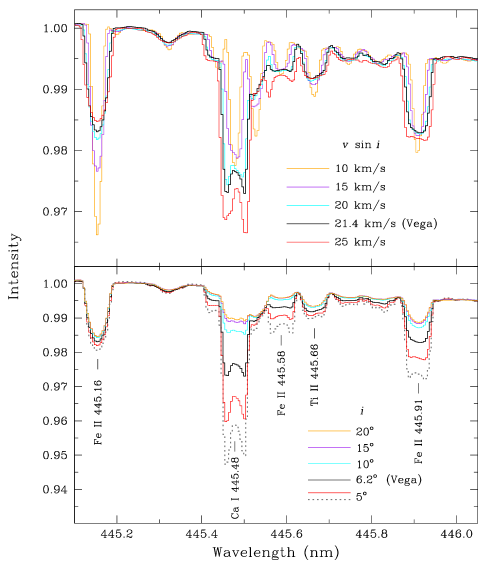
Figure 6 shows, as an illustrative example, the synthetic spectra of the two sets of models in a short wavelength interval between 445.0 and 446.0 nm. The upper and lower panels in the figure correspond to the models in the upper and lower parts of Table 2. The spectra have been normalised to the intensity at 445.2 nm and contain five lines: Fe ii 445.16, Ca i 445.48, Fe ii 445.58, Ti ii 445.66, and Fe ii 445.91 nm. The colour codes of the spectra — red, black, cyan, purple, and orange — correspond to decreasing values of (upper panel) and increasing values of inclinations (lower panel), the model for Vega being plotted in black.
What is interesting in this plot is how sensitive the profiles are to changes in inclination and , a conclusion that can be extended to the full spectral range. In particular, the profiles of the lines with peculiar shapes, as in the cases of Ca i 445.48, Fe ii 445.58, and Fe ii 445.91 nm, change very dramatically as the inclination decreases. Very interesting, too, is the comparison between the behaviour of the normal rounded-shape Fe ii 445.16 nm line and the peculiar Ca i 445.48 nm profile in the upper panel: whereas the Fe ii line behaves as one would expect as the value of increases, the shape and depth of the Ca i line changes drastically.
The model plotted as a dotted grey line in the lower panel has been computed for , , assuming the von Zeipel approximation; this model must be compared with the one plotted in red, computed with the same parameters, but under the assumptions of the -model. That value of would be associated with a exponent , quite far from . As can be inferred from the values of for both models in Table 2, the equator is almost 400 K cooler when the von Zeipel approximation is used, which results in deeper lines, in particular those with peculiar profiles, leading to erroneous determinations of abundances. This is a good example of the influence of the exponent on the line shapes and intensities.
All this shows the potential of a detailed spectral analysis to find structural and physical parameters and inclinations of this kind of stars. Good examples are the works by Takeda et al. (2008), Takeda (2020), and Takeda (2021) disentangling Sirius A and Vega’s properties using spectral line profiles, or Fourier analysis.
A quantitative analysis of the usefulness of the proposed formalisms is relevant. Regarding the inclination of the star, it is apparent that very clear changes are observed in certain line profiles as moves in the range between 0 and degrees; at larger inclinations, most of the lines are insensitive to this parameter. It is easy to prove that the probability of a star having an inclination between and is , and therefore the probability of finding a star, among a large set of objects with an inclination in the interval of [0,20] degrees is . As a first impression, one might consider the whole modelling effort to be disproportionate considering that the number is small; however, a query to the Gaia DR3 catalogue asking how many stars with spectral types between A0 and A9 — for which the methods presented here would be useful — with parallaxes, , with relative errors of , are ( mas) and ( mas). In other words, in a sphere with a radius of 1 kpc, we would find around stars in that range of spectral types with inclinations less than 20 degrees. The constraint of to bracket the interval A0-A9 has been used.333https://www.pas.rochester.edu/emamajek/
7 Conclusions
In this paper, we provide a combined method to compute the structure of rapidly rotating stars and build their synthetic spectra. A summary of the main features of the whole formalism follows:
-
1.
The -model by Espinosa Lara & Rieutord (2011) has been implemented to compute the relevant parameters of the photosphere of rapidly rotating stars — namely, the radius, , effective temperature, , and effective gravity, — as a function of the colatitude, . The method, relatively simple from a computational point of view, is able to reproduce the results of more complex models. One of the big advantages of this formalism is that it avoids the discussion, and hence the subsequent computation, or ad hoc assignment, of the appropriate gravity darkening exponent, . The model is applicable to stars with radiative envelopes (Sect. 3). In those situations in which some of the approximations inherent in the -model — that is, mass concentrated near the centre of the star and rigid rotation (Roche model) — are no longer valid, the original ESTER model should be used.
-
2.
A detailed method of how to compute the synthetic spectrum of a rapidly rotating star, at any inclination angle, , with respect to the line of sight, is presented. The model makes use of the suite of codes, atlas and synthe (Kurucz, 2014), and the grid of model atmospheres by Castelli & Kurucz (2003) (Sect. 4 and Appendices A and B).
-
3.
The combined methods summarised in items 1 and 2 above were applied to the particular case of Vega, obtaining results regarding both the structure and the synthetic spectrum that are compatible with previous works. The fitting of the spectral lines was remarkable, both for those with normal, rounded shapes and those with peculiar profiles (Sect. 5).
-
4.
In addition, Appendix A describes in detail how to treat, from a strict geometrical point of view, all the relevant variables when a rotating star is seen with a given inclination with respect to the line of sight.
Although this work has focused on the spectral synthesis of rapid rotators, the tools provided in this paper can be useful in other contexts:
- 1.
-
2.
To find and estimate the inclination of the rotation axis with respect to the line of sight in those cases without making use, in the first instance, of interferometric measurements (Takeda et al., 2008). This would be useful to search for potential pre-main-sequence stars of spectral types earlier than F hosting Jupiter-like planets. In particular, there is indirect evidence that Herbig Ae/Be stars with low metallicities could be good candidates to host such giant planets (Kama et al., 2015; Guzmán-Díaz et al., 2023). The method presented here would allow a detailed metallicity analysis, and a subsequent filtering of targets according to their inclination, which is suitable in the case of low-inclination systems of potential interferometric and/or direct imaging studies.
-
3.
The role of the inclination is particularly important in modelling accretion processes for young objects of intermediate mass. In the scenario of magnetospheric accretion, the shape and intensity of the spectral lines are strongly dependent on the assumed inclination (Muzerolle et al., 2004; Mendigutía et al., 2011). Regarding the alternative scenario of boundary layer continuum models, the dependence on the inclination is also critical (see e.g. Fig. 5 in Mendigutía, 2020).
Acknowledgements.
The author is very grateful to the referee, Prof. Michel Rieutord, and his colleagues, Alain Hui-Bon-Hoa and Axel Lazzarotto, for providing very useful comments, suggestions and references that, no doubt about, have improved the contents and scope of the paper. This research has been funded by grants AYA2014-55840-P, PGC2018-101950-B-I00 and PID2021-127289-NB-I00 by the Spanish Ministry of Science and Innovation/State Agency of Research (MCIN/AEI). The author is grateful to Francisco Espinosa-Lara for useful discussions on the ER11 formalism, Antonio Claret for some guiding for the computation of the limb-darkening coefficients, and Almudena Alonso-Herrero, Olga Balsalobre-Ruza, Carlos Eiroa, Jorge Lillo-Box, Ignacio Mendigutía, Enrique Solano and Eva Villaver for their help and comments to several sections of this paper. Special thanks also to Antonio Parras and Sergio Suárez for their work keeping up and running the computing centre.References
- Aufdenberg et al. (2006) Aufdenberg, J. P., Mérand, A., Coudé du Foresto, V., et al. 2006, ApJ, 645, 664
- Aumann et al. (1984) Aumann, H. H., Gillett, F. C., Beichman, C. A., et al. 1984, ApJ, 278, L23
- Bastian & de Mink (2009) Bastian, N. & de Mink, S. E. 2009, MNRAS, 398, L11
- Bessell (2005) Bessell, M. S. 2005, ARA&A, 43, 293
- Bouchaud et al. (2020) Bouchaud, K., Domiciano de Souza, A., Rieutord, M., Reese, D. R., & Kervella, P. 2020, A&A, 633, A78
- Castelli & Kurucz (2003) Castelli, F. & Kurucz, R. L. 2003, in Modelling of Stellar Atmospheres, ed. N. Piskunov, W. W. Weiss, & D. F. Gray, Vol. 210, A20
- Ciardi et al. (2001) Ciardi, D. R., van Belle, G. T., Akeson, R. L., et al. 2001, ApJ, 559, 1147
- Claret & Bloemen (2011a) Claret, A. & Bloemen, S. 2011a, A&A, 529, A75
- Claret & Bloemen (2011b) Claret, A. & Bloemen, S. 2011b, VizieR Online Data Catalog, J/A+A/529/A75
- Domiciano de Souza et al. (2014) Domiciano de Souza, A., Kervella, P., Moser Faes, D., et al. 2014, A&A, 569, A10
- Espinosa Lara & Rieutord (2011) Espinosa Lara, F. & Rieutord, M. 2011, A&A, 533, A43
- Espinosa Lara & Rieutord (2012) Espinosa Lara, F. & Rieutord, M. 2012, A&A, 547, A32
- Espinosa Lara & Rieutord (2013) Espinosa Lara, F. & Rieutord, M. 2013, A&A, 552, A35
- Girardi et al. (2019) Girardi, L., Costa, G., Chen, Y., et al. 2019, MNRAS, 488, 696
- Gray (1992) Gray, D. F. 1992, The Observation and Analysis of Stellar Photospheres, Cambridge University Press, 2nd edition
- Gulliver et al. (1991) Gulliver, A. F., Adelman, S. J., Cowley, C. R., & Fletcher, J. M. 1991, ApJ, 380, 223
- Guzmán-Díaz et al. (2023) Guzmán-Díaz, J., Montesinos, B., Mendigutía, I., et al. 2023, A&A, 671, A140
- Hanbury Brown et al. (1967) Hanbury Brown, R., Davis, J., Allen, L. R., & Rome, J. M. 1967, MNRAS, 137, 393
- Hill et al. (2004) Hill, G., Gulliver, A. F., & Adelman, S. J. 2004, in The A-Star Puzzle, ed. J. Zverko, J. Ziznovsky, S. J. Adelman, & W. W. Weiss, Vol. 224, 35–42
- Hill et al. (2010) Hill, G., Gulliver, A. F., & Adelman, S. J. 2010, ApJ, 712, 250
- Ilijic et al. (1998) Ilijic, S., Rosandic, M., Dominis, D., Planinic, M., & Pavlovski, K. 1998, Contributions of the Astronomical Observatory Skalnate Pleso, 27, 467
- Kama et al. (2015) Kama, M., Folsom, C. P., & Pinilla, P. 2015, A&A, 582, L10
- Kurucz (2014) Kurucz, R. L. 2014, in Determination of Atmospheric Parameters of B-,A-,F- and G-Type Stars. Series: GeoPlanet: Earth and Planetary Sciences, Springer International Publishing, 39–51
- Lazzarotto et al. (2023) Lazzarotto, A., Hui-Bon-Hoa, A., & Rieutord, M. 2023, A&A, 676, A50
- Lucy (1967) Lucy, L. B. 1967, ZAp, 65, 89
- Mendigutía (2020) Mendigutía, I. 2020, Galaxies, 8, 39
- Mendigutía et al. (2011) Mendigutía, I., Calvet, N., Montesinos, B., et al. 2011, A&A, 535, A99
- Millward & Walker (1985) Millward, C. G. & Walker, G. A. H. 1985, ApJS, 57, 63
- Monnier et al. (2012) Monnier, J. D., Che, X., Zhao, M., et al. 2012, ApJ, 761, L3
- Muzerolle et al. (2004) Muzerolle, J., D’Alessio, P., Calvet, N., & Hartmann, L. 2004, ApJ, 617, 406
- Pérez Hernández et al. (1999) Pérez Hernández, F., Claret, A., Hernández, M. M., & Michel, E. 1999, A&A, 346, 586
- Peterson et al. (2006) Peterson, D. M., Hummel, C. A., Pauls, T. A., et al. 2006, Nature, 440, 896
- Petrie (1964) Petrie, R. M. 1964, Publications of the Dominion Astrophysical Observatory Victoria, 12, 317
- Qiu et al. (2001) Qiu, H. M., Zhao, G., Chen, Y. Q., & Li, Z. W. 2001, ApJ, 548, 953
- Rieutord (2006) Rieutord, M. 2006, in SF2A-2006: Semaine de l’Astrophysique Francaise, ed. D. Barret, F. Casoli, G. Lagache, A. Lecavelier, & L. Pagani, 501
- Rieutord (2016) Rieutord, M. 2016, in Lecture Notes in Physics, Berlin Springer Verlag, ed. J.-P. Rozelot & C. Neiner, Vol. 914, 101
- Rieutord et al. (2016) Rieutord, M., Espinosa Lara, F., & Putigny, B. 2016, Journal of Computational Physics, 318, 277
- Sbordone (2005) Sbordone, L. 2005, Memorie della Societa Astronomica Italiana Supplementi, 8, 61
- Sibthorpe et al. (2010) Sibthorpe, B., Vandenbussche, B., Greaves, J. S., et al. 2010, A&A, 518, L130
- Takeda (2008) Takeda, Y. 2008, MNRAS, 388, 913
- Takeda (2020) Takeda, Y. 2020, MNRAS, 499, 1126
- Takeda (2021) Takeda, Y. 2021, MNRAS, 505, 1905
- Takeda et al. (2007) Takeda, Y., Kawanomoto, S., & Ohishi, N. 2007, PASJ, 59, 245
- Takeda et al. (2008) Takeda, Y., Kawanomoto, S., & Ohishi, N. 2008, ApJ, 678, 446
- von Zeipel (1924a) von Zeipel, H. 1924a, MNRAS, 84, 665
- von Zeipel (1924b) von Zeipel, H. 1924b, MNRAS, 84, 684
- Wheeler et al. (2023) Wheeler, A. J., Abruzzo, M. W., Casey, A. R., & Ness, M. K. 2023, AJ, 165, 68
- Yoon et al. (2010) Yoon, J., Peterson, D. M., Kurucz, R. L., & Zagarello, R. J. 2010, ApJ, 708, 71
Appendix A The geometry of the problem
According to the notation in Fig. 1, a point on the stellar surface with coordinates
when the star is seen equator-on, is transformed after a counterclockwise rotation around the axis by an angle, , is done, into by applying to the matrix ; namely,
| (10) |
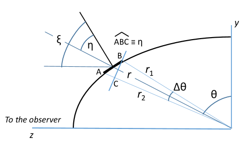
The observer would see all the points on the stellar surface fulfilling the easy constraint, . In the case of an spherical object, the unitary vector, , attached to any point has the direction of the normal to the surface; however, in an oblate object this is not the case, as can be seen in Fig. 7. The normal to the surface at a given point with colatitude , is inclined at an angle of with respect to the line of sight before proceeding to apply the rotation by an angle, . The computation of is a fairly straightforward geometrical problem, as is illustrated in the figure, in which has obviously been plotted out of scale: .
A differential surface area element at a latitude, , can be written as , and its associated unitary vector normal to the surface, before the star is rotated, has the following expression:
| (11) |
Therefore, after applying the rotation, the projected area as seen by the observer would be multiplied by the z-component of ; namely,
| (12) |
Concerning the rotation speed of each surface element, , it has only components and , as can be seen in Fig. 1 (left):
After applying the rotation, the component of the velocity in the line of sight is
| (13) |
Finally, the knowledge of the angle , between the normal to a given surface element and the line of sight, in the rotated system, must be known in order to apply the correction for limb darkening to the synthetic spectra arising from that surface element.
.
In the usual notation for that angle, , and according to Fig. 8, it can be written as , and since , the value of is just the component of ; namely,
| (14) |
Appendix B The limb-darkening coefficients
This appendix shows how the limb-darkening coefficients (LDCs hereafter) and the limb-darkening correction (see eqn. (7) are computed. The work and notation by Claret & Bloemen (2011a) are followed in this section. The LCDs are defined in such a way that the most general law is adjusted by the following expression:
| (15) |
is the intensity at the centre of the disc, and (see eqn. (14)), where is the angle between the normal to the surface area element and the line of sight. Equation (15) can be defined for the intensity in a given passband, although in our case we are interested in a monochromatic estimate of that quantity for each of the wavelengths covered by the synthetic spectra.
Claret & Bloemen (2011a) computed, among others, the LCDs for the photometric Johnson-Cousins filters (Table 17 available at Claret & Bloemen 2011b). In order to estimate the limb-darkening correction at each wavelength, , we linearly interpolate the LCDs in this way:
| (16) |
where F1 and F2 stand for ‘Filter 1’ and ‘Filter 2’ and , are the effective wavelengths of the filters adjacent to the wavelength, , under consideration; that is, . The wavelengths assigned to the filters for our computations are 360, 440, 550, 690, and 950 nm, respectively. Following that notation, the correction for limb-darkening applied to the fluxes at a given wavelength is
| (17) |