The $\ell$-test: leveraging sparsity in the Gaussian linear model for improved inference

Abstract

We develop novel LASSO-based methods for coefficient testing and confidence interval construction in the Gaussian linear model with $n\geq d$. Our methods’ finite-sample guarantees are identical to those of their ubiquitous ordinary-least-squares-$t$-test-based analogues, yet have substantially higher power when the true coefficient vector is sparse. In particular, our coefficient test, which we call the $\ell$-test, performs like the one-sided $t$-test (despite not being given any information about the sign) under sparsity, and the corresponding confidence intervals are more than 10% shorter than the standard $t$-test based intervals. The nature of the $\ell$-test directly provides a novel exact adjustment conditional on LASSO selection for post-selection inference, allowing for the construction of post-selection p-values and confidence intervals. None of our methods require resampling or Monte Carlo estimation. We perform a variety of simulations and a real data analysis on an HIV drug resistance data set to demonstrate the benefits of the $\ell$-test. We end with a discussion of how the $\ell$-test may asymptotically apply to a much more general class of parametric models.

1 Introduction

1.1 Motivation

Assume we have data $(\bm{y},\bm{X})$ from a (homoskedastic Gaussian) linear model:

$$\bm{y}\sim\mathcal{N}(\bm{X}\bm{\beta},\sigma^{2}\bm{I}),$$ (1.1)

where $\bm{X}\in\mathbb{R}^{n\times d}$ is full column-rank (and in particular, assume $n\geq d$) and treated as non-random, and $\bm{\beta}\in\mathbb{R}^{d}$ and $\sigma^{2}\in\mathbb{R}_{>0}$ are unknown. For a given covariate of interest $X_{j}$ this paper will consider testing $H_{j}:\beta_{j}=0$ and the related problem of constructing a confidence interval for $\beta_{j}$. It will leverage the LASSO to do so and our method’s construction will also make it easy to construct conditionally valid versions, conditioned on LASSO selection.

The go-to solution for this type of single covariate inference is based on the linear regression $t$-test for $H_{j}$, which can be efficiently inverted to obtain a $t$-test-based confidence interval for $\beta_{j}$. The linear regression $t$-test dates back over a century (Fisher, 1922) and is ubiquitous in introductory statistics courses and methods courses in nearly every domain of science and engineering. As a result, it is hard to overstate how universally widely used it is in practice. And it is easy to see why: the $t$-test is intuitive, easy to compute, and comes with strong theoretical guarantees.

The goal of this paper is to allow an analyst to leverage a belief in sparsity (of $\bm{\beta}$) to conduct more informative inference (when sparsity holds) without sacrificing the statistical guarantees of the $t$-test (even when sparsity does not hold). Sparsity is a widely held belief throughout applications in science and engineering (indeed, this belief is so ubiquitous that it has a name: the principle of parsimony), and while leveraging sparsity in regression is a heavily studied subject (we review existing approaches in Section 1.3), methods developed to leverage it often rely on sparsity for both validity and increased power, while we explicitly seek to rely on it only for increased power.

1.2 Summary of our contributions

We develop a hypothesis test for $H_{j}:\beta_{j}=0$, which we call the $\ell$-test, that uses the absolute value of the fitted LASSO coefficient as its test statistic. Using novel analysis of the conditional distribution of the LASSO estimator given the sufficient statistic of the linear model, we derive the test statistic’s exact null distribution, allowing us to efficiently compute p-values without resampling or Monte Carlo. We argue that the $\ell$-test will often achieve nearly the power of the one-sided $t$-test when $\bm{\beta}$ is sparse, despite not knowing the sign of $\beta_{j}$ and remaining exactly valid under identical assumptions as the two-sided $t$-test. We show the $\ell$-test can be efficiently inverted to produce exact confidence intervals, which due to the power improvement of the $\ell$-test are typically more than about 10% shorter than $t$-test-based confidence intervals when $\bm{\beta}$ is sparse. For both the $\ell$-test and its corresponding confidence interval, we show that a cross-validation procedure can be used to select the penalty parameter $\lambda$ in the LASSO from the data without impacting our validity guarantees, making our proposed procedures tuning-parameter-free. The nature of the $\ell$-test and our formula for its null distribution make it straightforward to derive and compute (novel) post-selection $\ell$-test p-values such that the post-selection $\ell$-test p-value for $H_{j}$ is exactly (and non-conservatively) valid conditional on the LASSO estimate of $\beta_{j}$ being nonzero; this conditional test can also be inverted to construct a confidence interval that is valid conditional on selection. A wide range of simulations and an application to HIV drug resistance demonstrate our methods to be powerful, efficient, and robust. In our discussion, we point out that the $\ell$-test can be directly generalized to any normal means problem with known covariance, and hence in particular should be applicable to any parametric model’s maximum likelihood estimator in its asymptotic Gaussian limit.

1.3 Related work

The standard choice for testing $H_{j}:\beta_{j}=0$ (and, via inversion, constructing confidence intervals) in the linear model is the (two-sided) $t$-test, or the one-sided $t$-test when the sign is known. Given the age and ubiquity of the linear model in statistics, we do not attempt to cover all related literature (though Lei and Bickel (2020), particularly their Appendix B, provides an excellent and detailed review), but just note that many such works focus on developing methods with some form of guarantees under weaker assumptions than the standard (homoskedastic) Gaussian linear model assumed in this paper (Friedman, 1937, Pitman, 1937, 1938, Kruskal and Wallis, 1952, Tukey, 1958, Hajek, 1962, Adichie, 1967, Jaeckel, 1972, Efron, 1979, Freedman, 1981, Gutenbrunner et al., 1993, Lei and Bickel, 2020). As their goal is robustness, these methods generally do not outperform the $t$-test in the (homoskedastic) Gaussian linear model, whereas this is exactly the goal of the current paper: maintain the same guarantees as the $t$-test while improving its power when $\bm{\beta}$ is sparse. To our knowledge, the only other work that leverages a linear model’s sparsity for testing an individual coefficient is the de-biased LASSO (van de Geer et al., 2014, Zhang and Zhang, 2014, Javanmard and Montanari, 2014), but, when $n\geq d$, it either reduces exactly to the $t$-test or is only asymptotically valid under strong sparsity assumptions on $\bm{\beta}$; in contrast, the validity of the $\ell$-test holds regardless of the sparsity of $\bm{\beta}$. There are a number of excellent works that aim to leverage sparsity for more powerful inference in the Gaussian linear model, including (fixed-X) knockoffs (Barber and Candès, 2015) and subsequent follow-ups that improve its performance (e.g., Spector and Janson (2022), Luo et al. (2022), Ren and Barber (2023), Lee and Ren (2024)), as well as methods based on mirror statistics (Xing et al., 2023, Dai et al., 2022), but all of these methods can only be used for variable selection and do not provide single-variable inference.

Two approaches share a similar goal as ours in seeking to improve the $t$-test’s power without making further assumptions. The first approach is Habiger and Peña (2014), which proposes to split the observations into two disjoint (thus independent) parts and uses the first part to estimate the sign of $\beta_{j}$ and then leverages the estimated sign in a test using the second part of the data. As we will discuss in Section 2.2, the $\ell$-test also leverages an estimated sign of $\beta_{j}$, but since it does not involve data splitting, it does not suffer from the associated loss in sample size and power. The second approach is called Frequentist, assisted by Bayes (FAB), which, given a prior on $\bm{\beta}$ and $\sigma^{2}$, produces Bayes-optimal power (or confidence interval width) subject to maintaining the same frequentist validity as the $t$-test (Hoff and Yu, 2019). But this paper only considers (dense) Gaussian priors for $\bm{\beta}$ and hence, unlike the $\ell$-test, does not leverage sparsity.

While the goal of the $\ell$-test is most similar to the works mentioned so far, its approach is most closely related to the idea of conditioning on a sufficient statistic under the null hypothesis. This approach is perhaps most prominently used in constructing uniformly most powerful unbiased tests (Lehmann and Scheffé, 1955), including the $t$-test. But this idea is also fundamental to co-sufficient sampling (Bartlett, 1937, Stephens, 2012), which is used for testing in a wide variety of contexts; see Barber and Janson (2022) for a recent review of such tests. However, the $\ell$-test is not sampling-based, and besides, to the best of our knowledge, the only work applying co-sufficient sampling to testing in the linear model is Huang and Janson (2020), but there it is applied to knockoffs (Barber and Candès, 2015, Candès et al., 2018) which is a method for variable selection and cannot perform single-coefficient inference.

Related to this paper’s post-selection inference methods, there is a rich literature on obtaining p-values that are valid post-selection (Cox, 1975, Berk et al., 2013, Fithian et al., 2014, Rinaldo et al., 2016, Bachoc et al., 2016, Tian and Taylor, 2018) and in particular in the linear model conditioned on LASSO selection (Lee et al., 2016, Tibshirani et al., 2016, Liu et al., 2018, Panigrahi et al., 2021). Closest to our work is Liu et al. (2018), which can be thought of as adjusting the standard $t$-test (or, more accurately, the $z$-test, since they assume $\sigma^{2}$ known) for a coefficient to make it valid conditional on that coefficient being selected by the LASSO. The conditional $\ell$-test can be thought of as making an analogous adjustment to the $\ell$-test rather than the $t$-test, resulting in similar gains under sparsity over Liu et al. (2018)’s method as the unconditional $\ell$-test achieves over the standard $t$-test; see Sections 4, 5.4, and Appendix F.4 for further comparison and discussion.

1.4 Notation

Throughout this paper, we will use boldfaced symbols to denote matrices and vectors. For a matrix $\bm{A}$, unless otherwise stated, $\bm{A}_{j}$ denotes its $j^{\mathrm{th}}$ column, $\bm{A}_{-j}$ denotes its sub-matrix with the $j^{\mathrm{th}}$ column dropped while $A_{ij}$ (note the symbol is no longer boldfaced) denotes the entry in the $i^{\mathrm{th}}$ row and the $j^{\mathrm{th}}$ column. Similarly for a vector $\bm{a}\in\mathbb{R}^{d}$, unless otherwise stated, $a_{j}$ denotes its $j^{\mathrm{th}}$ entry while $\bm{a}_{-j}$ denotes the sub-vector of $\bm{a}$ without the $j^{\mathrm{th}}$ entry. We will also use $\mathbb{I}(\cdot)$ as the indicator function that takes the value 1 if the condition within the parantheses is true, and 0 otherwise.

1.5 Software

Functions in R (R Core Team, 2024) for running all methods in this paper are available at github.com/SSouhardya/l-test.

2 The $\ell$-test

Our proposed test for $H_{j}:\beta_{j}=0$ is primarily based on the simple idea of conditioning on sufficient statistics. The minimal sufficient statistic for the linear model under $H_{j}$ is $\bm{S}^{(j)}:=(\bm{X}_{-j}^{T}\bm{y},\bm{y}^{T}\bm{y})$. So, by sufficiency, the conditional distribution of $\bm{y}\mid\bm{S}^{(j)}$ does not depend on any unknown parameters under $H_{j}$, and the same holds true for the conditional distribution of any fixed function of $\bm{y}$, including the LASSO coefficient estimate. Let

$$\hat{\bm{\beta}}^{\lambda}=\underset{\bm{\beta}}{\arg\min}\left(\frac{1}{2n}\|\bm{y}-\bm{X}\bm{\beta}\|^{2}+\lambda\sum_{k}|\beta_{k}|\right)$$

denote the LASSO estimator of the entire coefficient vector with penalty parameter $\lambda$. Denote the cumulative distribution function (CDF) for the conditional distribution of $\hat{\beta}^{\lambda}_{j}\mid\bm{S}^{(j)}$ under $H_{j}$, which we call the $\ell$-distribution, evaluated at some $b\in\mathbb{R}$, by

$$F^{\lambda}_{\ell}(b\mid\bm{S}^{(j)}):=\mathbb{P}_{H_{j}}(\hat{\beta}^{\lambda}_{j}\leq b\mid\bm{S}^{(j)}).$$

By sufficiency, the $\ell$-distribution does not depend on any unknown parameters under $H_{j}$, and hence we can in principle compute a valid p-value for $H_{j}$ that rejects for large $|\hat{\beta}^{\lambda}_{j}|$:

$$\bar{F}_{|\ell|}^{\lambda}(|\hat{\beta}^{\lambda}_{j}|\mid\bm{S}^{(j)}),$$

where $\bar{F}_{|\ell|}^{\lambda}(b\mid\bm{S}^{(j)}):=\mathbb{P}_{H_{j}}(|\hat{\beta}^{\lambda}_{j}|\geq b\mid\bm{S}^{(j)})=1-\lim_{b^{\prime}\rightarrow b^{-}}F_{\ell}^{\lambda}(b^{\prime}\mid\bm{S}^{(j)})+F^{\lambda}_{\ell}(-b\mid\bm{S}^{(j)})$ denotes the tail probability of $|\hat{\beta}^{\lambda}_{j}|$ and is entirely determined by the $\ell$-distribution $F_{\ell}^{\lambda}$. We call the test that uses the above p-value the $\ell$-test, though our recommended usage of it involves two modifications, one about breaking ties in the p-value when $\hat{\beta}_{j}^{\lambda}=0$ (which currently cause a point mass at 1 in the p-value distribution) and the other about the choice of $\lambda$. We defer these two choices to Sections 2.3 and 2.4, respectively, and first provide a characterization of the $\ell$-distribution which allows us to efficiently compute the $\ell$-test p-value and helps explain why, when, and by how much the $\ell$-test increases power over the $t$-test.

2.1 The $\ell$-distribution

As the first step towards characterizing the $\ell$-distribution $F^{\lambda}_{\ell}(\cdot\mid\bm{S}^{(j)})$, we restate (Luo et al., 2022, Proposition E.1) that exactly characterizes the distribution of $\bm{y}\mid\bm{S}^{(j)}$ under $H_{j}$. Let $\bm{P}_{-j}=\bm{X}_{-j}(\bm{X}_{-j}^{T}\bm{X}_{-j})^{-1}\bm{X}_{-j}^{T}$ denote the projection matrix onto the column space of $\bm{X}_{-j}$.

Lemma 2.1 (Luo et al. (2022)).

For the Gaussian linear model (1.1), define $\hat{\bm{y}}_{j}=\bm{P}_{-j}\bm{y}$ and $\hat{\sigma}_{j}^{2}=\|\bm{y}-\hat{\bm{y}}_{j}\|^{2}$, and let $\bm{V}\in\mathbb{R}^{n\times(n-d+1)}$ denote an orthonormal matrix orthogonal to the column space of $\bm{X}_{-j}$ with first column given by $\bm{V}_{1}=\frac{(\bm{I}-\bm{P}_{-j})\bm{X}_{j}}{\|(\bm{I}-\bm{P}_{-j})\bm{X}_{j}\|}$. Then, there exists a unique vector $\bm{u}\in\mathbb{R}^{n-d+1}$, such that $\|\bm{u}\|=1$ and the following relation holds:

$$\bm{y}=\hat{\bm{y}}_{j}+\hat{\sigma}_{j}\bm{V}\bm{u}.$$ (2.1)

Furthermore, under $H_{j}$,

$$\bm{u}\mid\bm{S}^{(j)}\sim\mathrm{Unif}\left(\mathbb{S}^{n-d}\right),$$ (2.2)

where $\mathbb{S}^{n-d}$ denotes the unit sphere of dimension $n-d$.

For completeness, a proof of the lemma is provided in Section C.1 of the Appendix. Next our main theoretical result, Theorem 2.1, establishes a mapping between $\hat{\beta}_{j}^{\lambda}$ and just the first element of $\bm{u}$, $u_{1}$ (there is nothing special about index 1 here except that we defined $\bm{V}$ to have only its first column non-orthogonal to $\bm{X}_{j}$), which will give an immediate characterization of $F_{\ell}^{\lambda}$ via the known distribution of $u_{1}$ from Equation (2.2).

Theorem 2.1 (Characterization of the $\ell$-distribution).

Consider the unique decomposition (2.1) from Lemma 2.1 and for any $b\in\mathbb{R}$ and $\epsilon\in\{-1,1\}$, define the functions

$$\hat{\bm{\beta}}^{\lambda}_{-j}(b):=\underset{\bm{\beta}_{-j}\in\mathbb{R}^{d-1}}{\arg\min}\left(\frac{1}{2n}\|\bm{y}-b\bm{X}_{j}-\bm{X}_{-j}\bm{\beta}_{-j}\|^{2}+\lambda\|\bm{\beta}_{-j}\|_{1}\right),$$ (2.3)

$$\Lambda_{j}(b,\epsilon)=\frac{-\bm{X}_{j}^{T}\left(\hat{\bm{y}}_{j}-b\bm{X}_{j}-\bm{X}_{-j}\hat{\bm{\beta}}_{-j}(b)\right)+n\lambda\epsilon}{\hat{\sigma}_{j}\|(\bm{I}-\bm{P}_{-j})\bm{X}_{j}\|}.$$

Then the function $f_{\bm{S}^{(j)}}:\mathbb{R}\mapsto\mathbb{R}$, defined via its inverse as

$$f_{\bm{S}^{(j)}}^{-1}(b)=\begin{cases}\Lambda_{j}(b,\mathrm{sign}(b)),&\text{if }b\neq 0\\ [\Lambda_{j}(0,-1),\Lambda_{j}(0,1)],&\text{if }b=0\end{cases},$$ (2.4)

satisfies $\hat{\beta}_{j}^{\lambda}=f_{\bm{S}^{(j)}}(u_{1})$ and is continuous and non-decreasing in its domain, and strictly increasing on the set $\{u:f_{\bm{S}^{(j)}}(u)\neq 0\}$.

Theorem 2.1 exactly characterizes the $\ell$-distribution: for $b\neq 0$, we have

$$\{\hat{\beta}_{j}^{\lambda}\leq b\}=\left\{f_{\bm{S}^{(j)}}^{-1}\left(\hat{\beta}_{j}^{\lambda}\right)\leq f_{\bm{S}^{(j)}}^{-1}\left(b\right)\right\}=\left\{u_{1}\leq\Lambda_{j}(b,\mathrm{sign}(b))\right\}.$$ (2.5)

Thus, in particular, if we let $F_{u}$ denote the CDF of $u_{1}$ under $H_{j}$, then $F_{\ell}^{\lambda}(b)=\mathbb{P}_{H_{j}}(\hat{\beta}_{j}^{\lambda}\leq b\mid\bm{S}^{(j)})=F_{u}(\Lambda_{j}(b,\mathrm{sign}(b)))$ because $\Lambda_{j}(b,\mathrm{sign}(b))$ is a function of $\bm{S}^{(j)}$ for any fixed $b$. Similarly, for $b=0$, it follows from Theorem 2.1 that $F_{\ell}^{\lambda}(0)=F_{u}\left(\Lambda_{j}(0,1)\right)$. Note that $F_{u}$ is easily evaluated via a one-to-one mapping to a $t$-distribution, namely, $\frac{\sqrt{n-d}u_{1}}{\sqrt{1-u_{1}^{2}}}\sim t_{n-d}$ (see Appendix C.5 for a proof), which, along with the relations above, can be used to explicitly calculate quantiles of the $\ell$-distribution. The proof of Theorem 2.1 in Appendix C.3 hinges on two main ideas—first, we use blockwise coordinate descent to characterize the event $\{\hat{\beta}_{j}^{\lambda}=b\}$ in terms of $u_{1}$, and second, we characterize $f_{\bm{S}^{(j)}}$ by obtaining an exact expression for $\frac{\partial}{\partial u_{1}}f_{\bm{S}^{(j)}}$, which turns out to be non-negative throughout, thereby showing $f_{\bm{S}^{(j)}}$ is non-decreasing. We will see next that Theorem 2.1 also provides critical insights into the power of the $\ell$-test.

2.2 The power of the $\ell$-test

Our simulations in Section 5.1 show that not only does the $\ell$-test consistently beat the usual two-sided $t$-test when $\bm{\beta}$ is sparse, it achieves power close to the one-sided $t$-test (in the correct direction), being nearly identical in some cases, without any knowledge about the true sign of $\beta_{j}$.

To explain this behavior, we first characterize the relationship between the $t$-test statistic and $u_{1}$ in Lemma 2.2. It turns out that $u_{1}$ is a scalar multiple of $\bm{X}_{j}^{T}(\bm{I}-\bm{P}_{-j})\bm{y}$ (we argue this in Equations (C.1) through (C.4) of the Appendix and is a major component in the proof of the lemma), and hence, $u_{1}$ is a measure of the association between $\bm{X}_{j}$ and the component of $\bm{y}$ that cannot be explained by the rest of the columns.

Lemma 2.2.

Let $T_{j}$ denote the $t$-test statistic for testing $H_{j}:\beta_{j}=0$. Then, there exists a continuous, strictly increasing, anti-symmetric function $g_{\bm{S}^{(j)}}$ that is a functional of the sufficient statistic $\bm{S}^{(j)}$, such that $T_{j}=g_{\bm{S}^{(j)}}(u_{1})$.

We prove this result in Section C.2 of the appendix. Lemma 2.2 and Theorem 2.1 together show that a (one-sided) conditional-on-$\bm{S}^{(j)}$ test based on any of the test-statistics—$u_{1},T_{j}$ and $\hat{\beta}_{j}^{\lambda}$, yield exactly the same p-values as long as the observed LASSO estimate is non-zero, as in this case all the three test statistics are strictly increasing in each other. We also know that $T_{j}$ is independent of $\bm{S}^{(j)}$, which follows from standard theory on ancillary statistics, however we supply a separate proof for this in Section C.4 of the Appendix. This implies that a one-sided conditional test based on $T_{j}\mid\bm{S}^{(j)}$ yields exactly the one-sided $t$-test p-value, which by the above argument is exactly equal to the one-sided p-value of the conditional test based on $\hat{\beta}^{\lambda}_{j}\mid\bm{S}^{(j)}$ when the observed LASSO estimate is non-zero.

Even though the above paragraph establishes that conditional one-sided testing based on $\hat{\beta}^{\lambda}_{j}$ can do only as well as the corresponding one-sided $t$-test, we will now argue that the former test can gain considerable power over the $t$-test in the two-sided testing regime. As a first step, note that we can use Theorem 2.1 to characterize the set $\mathcal{R}:=\{u_{1}:\hat{\beta}_{j}^{\lambda}\neq 0\}$ as a disjoint union of two intervals: $\mathcal{R}=(-\infty,v_{-})\cup(v_{+},\infty)$, where, $v_{\pm}=\Lambda_{j}(0,\pm 1)$.

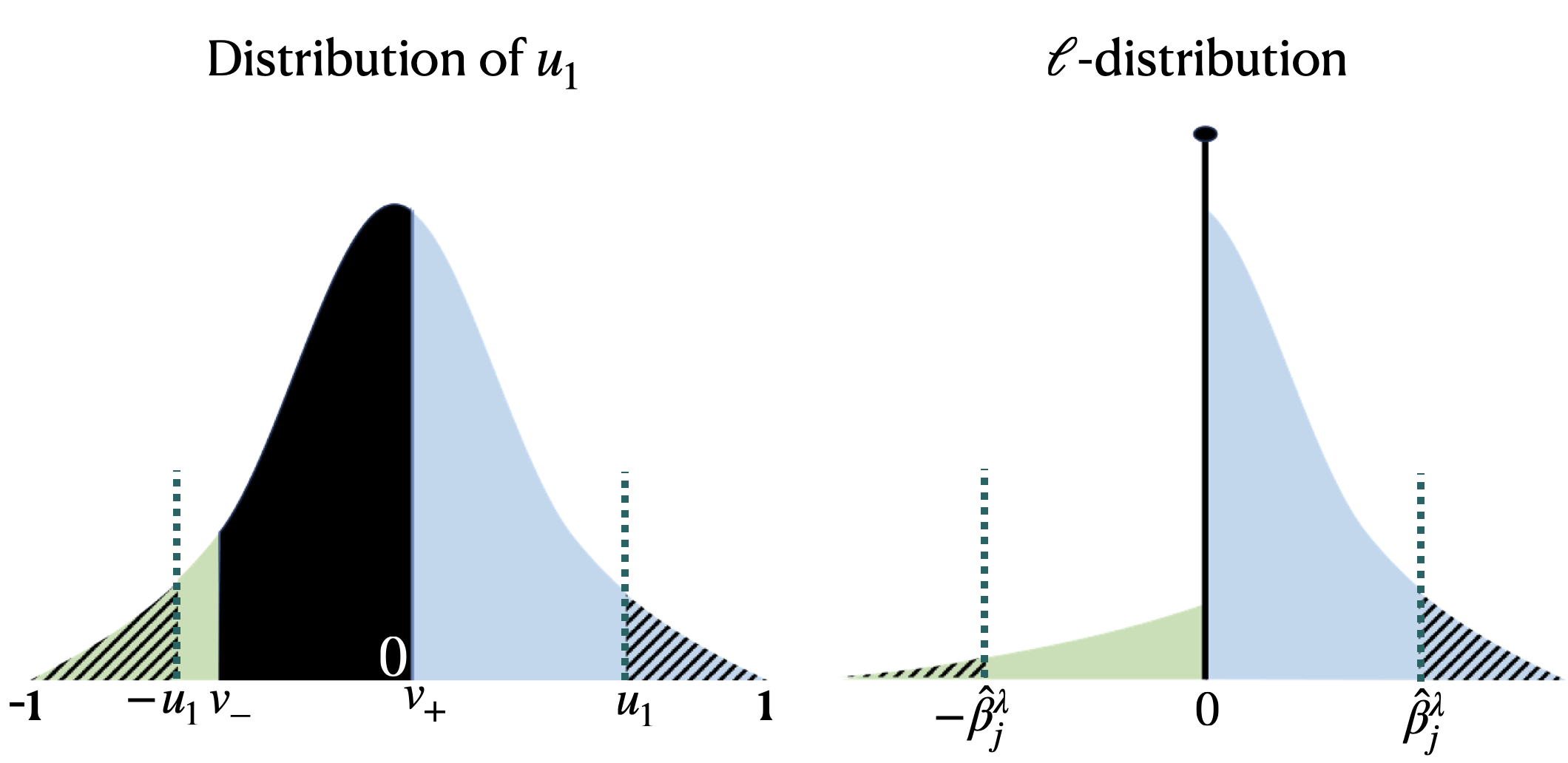
Figure 1: Connection between the distribution of $u_{1}$ (left) and the $\ell$-distribution (right). Regions of matching color between the two plots represent a one-to-one correspondence between the random variable values within them, as proved in Theorem 2.1.

We will argue that when $\beta_{j}\neq 0$, the test based on $|\hat{\beta}^{\lambda}_{j}|$ (i.e., the $\ell$-test) leverages the asymmetry of the interval $[v_{-},v_{+}]$ about 0 to gain power. Observe that from Theorem 2.1, $\hat{\beta}_{j}^{\lambda}$ is negative when $u_{1}\leq v_{-}$, while it is positive when $u_{1}\geq v_{+}$. Without loss of generality, we will assume that $\beta_{j}>0$ for the proceeding discussion, and assume the center of the interval $[v_{-},v_{+}]$ is negative (we will justify this latter assumption in a little bit). Consider Figure 1 for a visual representation of this, where under $H_{j}$, the left and the right figures show the conditional distributions of $u_{1}$ (i.e., $F_{u}$) and $\hat{\beta}_{j}^{\lambda}$ (i.e., the $\ell$-distribution $F_{\ell}^{\lambda}(\cdot\mid\bm{S}^{(j)})$), respectively. The correspondence between the two distributions is shown by matching colors—for example, as is evident from Theorem 2.1, the mass that the distribution of $u_{1}$ puts to the left of $v_{-}$ is exactly the mass the $\ell$-distribution puts on the negative half, and hence both these regions are colored green. As can be seen from the figure, the asymmetry in $[v_{-},v_{+}]$ (and the symmetry of $F_{u}$) directly implies asymmetry in the $\ell$-distribution.

Since $\beta_{j}>0$, we expect that $\hat{\beta}_{j}^{\lambda}>0$ as well, as reflected in the righthand plot, with corresponding positive $u_{1}$ also marked in the lefthand plot. Due to the symmetry of $u_{1}$’s distribution, the p-value of the two-sided test using $|u_{1}|$ is just twice the mass to the right of $u_{1}$, and by Lemma 2.2, this is also the p-value of the (two-sided) $t$-test. To understand the $\ell$-test p-value for comparison, note that by Theorem 2.1, the mass to the right of $u_{1}$ in the left plot is exactly the mass to the right of $\hat{\beta}^{\lambda}_{j}$ in the right plot, but, critically, the mass to the left of $-\hat{\beta}^{\lambda}_{j}$ in the right plot is far less than the mass to the left of $-u_{1}$ in the left plot. Thus, the $\ell$-test’s p-value, which is exactly the mass of the shaded regions in the right plot, is dominated by the right-most shaded region, whose mass is exactly the value of the one-sided $t$-test.

Next, we argue why we expect the interval $[v_{-},v_{+}]$ to lean opposite to the true sign of $\beta_{j}$, that is, towards the negative side in this case. Note that the interval $[v_{-},v_{+}]$ has mid-point

$$\hat{m}_{j}:=\frac{v_{-}+v_{+}}{2}=\frac{\Lambda_{j}(0,-1)+\Lambda_{j}(0,+1)}{2}=\frac{-\bm{X}_{j}^{T}\left(\hat{\bm{y}}_{j}-\bm{X}_{-j}\hat{\bm{\beta}}^{\lambda}_{-j}(0)\right)}{\|(\bm{I}-\bm{P}_{-j})\bm{X}_{j}\|\hat{\sigma}_{j}}.$$ (2.6)

We can think of $\hat{m}_{j}$ as an estimator of $m_{j}$, where $m_{j}$ has the exact same expression with $\hat{\bm{\beta}}^{\lambda}_{-j}(0)$ replaced by its estimand, $\bm{\beta}_{-j}$. Defining $\tau_{j}^{2}:=\bm{X}_{j}^{T}\bm{P}_{-j}\bm{X}_{j}\geq 0$, it can be seen that the numerator of $m_{j}$ satisfies

$$-\bm{X}_{j}^{T}(\hat{\bm{y}}_{j}-\bm{X}_{-j}\bm{\beta}_{-j})\sim\mathcal{N}\left(-\beta_{j}\tau_{j}^{2},\sigma^{2}\tau_{j}^{2}\right).$$

Thus under the alternative, $m_{j}$’s distribution is shifted towards the opposite sign of $\beta_{j}$ as long as $\bm{X}_{j}$ is not exactly orthogonal to $\bm{X}_{-j}$. And when $\bm{\beta}$ is sparse, we expect the lasso estimator $\hat{\bm{\beta}}_{-j}^{\lambda}(0)$ of $\bm{\beta}_{-j}$ to be a good one, and hence that $\hat{m}_{j}$’s distribution will also be shifted towards the opposite sign of $\beta_{j}$. In particular, when $\beta_{j}>0$, this means we expect $[v_{-},v_{+}]$ to be shifted in the negative direction, as we assumed it would be earlier in this subsection.

In sum, when $\bm{\beta}$ is sparse, the LASSO leverages information in $\bm{S}^{(j)}$ (via $\hat{\bm{\beta}}_{-j}^{\lambda}(0)$) to guess the sign of $\beta_{j}$, and the point mass in the $\ell$-distribution uses that guess (via $[v_{-},v_{+}]$) to reduce the “wrong” tail of the $\ell$-test, resulting in a test with power approximating the one-sided $t$-test; see Appendix B for further discussion. Note that although the intuition for the power gain of the $\ell$-test over the $t$-test relied on sparsity, we emphasize that the validity guarantees of the $\ell$-test remain identical to those of the $t$-test, and in particular do not require sparsity.

2.3 Breaking ties when $\hat{\beta}_{j}^{\lambda}=0$

As alluded to earlier in this section, the $\ell$-test p-value $\bar{F}_{|\ell|}^{\lambda}(|\hat{\beta}^{\lambda}_{j}|\mid\bm{S}^{(j)})$ is not $\mathrm{Unif}(0,1)$ under $H_{j}$. Instead, its conditional distribution given $\bm{S}^{(j)}$ is a mixture of $\mathrm{Unif}(0,\mathbb{P}_{H_{j}}(\hat{\beta}_{j}^{\lambda}\neq 0\mid\bm{S}^{(j)}))$ and a point mass at 1 of weight $\mathbb{P}_{H_{j}}(\hat{\beta}_{j}^{\lambda}=0\mid\bm{S}^{(j)})$ because $|\hat{\beta}_{j}^{\lambda}|=0$ is the “least significant” value of the test statistic and occurs with positive probability. It is preferable not to have such a point mass, since it makes the $\ell$-test somewhat conservative and because both users and many procedures which take p-values as inputs generally assume uniform null p-values. To remedy this, we need a way to break ties among data values that give $\hat{\beta}_{j}^{\lambda}=0$, since the test statistic $|\hat{\beta}_{j}^{\lambda}|$ does not distinguish between them. The strong connection between $\hat{\beta}_{j}^{\lambda}$ and $u_{1}$ established in Theorem 2.1 and visualized in Figure 1 suggests that $u_{1}$, whose distribution is continuous on $[v_{-},v_{+}]$ given the event $\{\hat{\beta}_{j}^{\lambda}=0\}$, provides a way forward. In particular, since $\hat{\beta}_{j}^{\lambda}$ approaches zero as $u_{1}$ approaches $v_{-}$ from the left or $v_{+}$ from the right, it is natural (and continuous in the data) to set $v_{-}$ and $v_{+}$ as tied for the “most significant” values on the interval $[v_{-},v_{+}]$, and then have the significance decrease as $u_{1}$ moves inward from those endpoints. This corresponds to breaking ties according to $|u_{1}-\hat{m}_{j}|$ when $\hat{\beta}_{j}^{\lambda}=0$, and can equivalently be thought of as using $|\hat{\beta}_{j}^{\lambda}|+\min\{|u_{1}-\hat{m}_{j}|-(v_{+}-\hat{m}_{j}),0\}$ as the test statistic. Recalling that $F_{u}$ denotes $u_{1}$’s CDF and defining $\bar{F}_{|u|}(u^{\prime}\mid\bm{S}^{(j)}):=\mathbb{P}_{H_{j}}(|u_{1}-\hat{m}_{j}|\geq u^{\prime}\mid\bm{S}^{(j)})=1-F_{u}(\hat{m}_{j}+u^{\prime})+F_{u}(\hat{m}_{j}-u^{\prime})$ as the tail probability of $|u_{1}-\hat{m}_{j}|$, we can express this p-value as

$$p^{\lambda}_{j}:=\begin{cases}\bar{F}_{|\ell|}^{\lambda}(|\hat{\beta}^{\lambda}_{j}|\mid\bm{S}^{(j)}),&\textrm{ if }\hat{\beta}^{\lambda}_{j}\neq 0\\ \bar{F}_{|u|}\left(|u_{1}-\hat{m}_{j}|\mid\bm{S}^{(j)}\right),&\textrm{ if }\hat{\beta}^{\lambda}_{j}=0\end{cases},$$ (2.7)

which is exactly $\mathrm{Unif}(0,1)$ under $H_{j}$ and never larger than $\bar{F}_{|\ell|}^{\lambda}(|\hat{\beta}^{\lambda}_{j}|\mid\bm{S}^{(j)})$, the p-value proposed in Section 2.1.

2.4 The choice of $\lambda$

Thus far, we have treated $\lambda$ as a fixed tuning parameter, but in practice it is preferable to have an automated, data-dependent way to choose it. Standard practice for the LASSO is to choose $\lambda$ via cross-validation (on the full data $(\bm{y},\bm{X})$), but while this choice invalidates the theoretical guarantees of the $\ell$-test, just a slight modification of it is sufficient to retain those guarantees. Let $\tilde{\bm{u}}\sim\mathrm{Unif}(\mathbb{S}^{n-d})$ be drawn independently of $\bm{u}$, and plug it into Equation (2.1) and call the resulting lefthand side $\tilde{\bm{y}}$, so that $\tilde{\bm{y}}$ is conditionally independent of $\bm{y}$ given $\bm{S}^{(j)}$. Then it is easy to see that cross-validation on $(\tilde{\bm{y}},\bm{X}_{-j})$ produces a $\lambda$, which we denote by $\hat{\lambda}_{j}$, that is exactly valid to use in the $\ell$-test, since conditioning on $\hat{\lambda}_{j}$ does not change the $\ell$-distribution. And empirically, $\hat{\lambda}_{j}$ (our implementation uses 10-fold cross-validation) seems to be just as powerful as the (technically invalid) choice via cross-validation on $(\bm{y},\bm{X})$; see Appendix E.2. Although $\hat{\lambda}_{j}$ is randomized through $\tilde{\bm{u}}$ and the random 10-fold partition of the data used by cross-validation, we find this exogenous randomness barely makes a difference: in our simulations it empirically accounts for at most about 0.8% of the variability in the $\ell$-test p-value $p_{j}^{\hat{\lambda}_{j}}$; see Appendix E.2. Furthermore, if desired, this randomness could be arbitrarily reduced by computing many conditionally independent $\hat{\lambda}_{j}$’s and using their mean or median for the $\ell$-test.

2.5 Putting it all together: the $\ell$-test

We can now state our recommended implementation of the $\ell$-test: the p-value $p_{j}^{\hat{\lambda}_{j}}$ which combines the main $\ell$-test idea with the tie-breaking of Sections 2.3 and the $\lambda$ choice of Section 2.4. Computing $p_{j}^{\hat{\lambda}_{j}}$ requires, aside from a cross-validated LASSO to compute $\hat{\lambda}_{j}$, one (non-cross-validated) LASSO to compute $\hat{\bm{\beta}}^{\hat{\lambda}_{j}}$ and, if $\hat{\beta}_{j}^{\hat{\lambda}_{j}}\neq 0$, then a second (non-cross-validated) LASSO to compute $\hat{\bm{\beta}}_{-j}^{\hat{\lambda}_{j}}(-\hat{\beta}_{j}^{\hat{\lambda}_{j}})$. When $\hat{\beta}_{j}^{\hat{\lambda}_{j}}\neq 0$, these two LASSO’s allow us to compute the two tails for the $\ell$-test p-value via Theorem 2.1, since $\hat{\bm{\beta}}_{-j}^{\hat{\lambda}_{j}}(\hat{\beta}_{j}^{\hat{\lambda}_{j}})=\hat{\bm{\beta}}_{-j}^{\hat{\lambda}_{j}}$. And when $\hat{\beta}_{j}^{\hat{\lambda}_{j}}=0$, by Equation (2.7), the only LASSO quantity needed is $\hat{\bm{\beta}}_{-j}^{\hat{\lambda}_{j}}(0)$ to compute $\hat{m}_{j}$, but since $\hat{\bm{\beta}}_{-j}^{\hat{\lambda}_{j}}(0)=\hat{\bm{\beta}}_{-j}^{\hat{\lambda}_{j}}$ in this case, no additional LASSO run is needed beyond the first. Thus computation for the $\ell$-test requires just a very small constant number of LASSO runs.

It is an immediate consequence of our construction that $p_{j}^{\hat{\lambda}_{j}}$ is valid and non-conservative under no further assumptions than the (homoskedastic Gaussian) linear model, which we formally state here as a corollary.

Corollary 2.1 (Validity of the $\ell$-test).

For model (1.1), for all $\alpha\in[0,1]$, $\mathbb{P}_{H_{j}}(p_{j}^{\hat{\lambda}_{j}}\leq\alpha)=\alpha$.

3 $\ell$-test confidence intervals

If we can use the $\ell$-test to test $H_{j}(\gamma):\beta_{j}=\gamma$ for any $\gamma\in\mathbb{R}$, then this family of tests can be inverted to obtain a valid confidence region for $\beta_{j}$. But extending the $\ell$-test to $H_{j}(\gamma)$ is straightforward, since $\bm{y}$ satisfying $H_{j}(\gamma)$ is equivalent to $\bm{y}-\gamma\bm{X}_{j}$ satisfying $H_{j}(0)=H_{j}$, so we can simply apply the regular $\ell$-test (exactly as detailed in Section 2) to the data $(\bm{y}-\gamma\bm{X}_{j},\bm{X})$. Defining $p_{j}^{\hat{\lambda}_{j}(\gamma)}(\gamma)$ as the $\ell$-test p-value for $H_{j}(\gamma)$, the $100(1-\alpha)\%$ $\ell$-test confidence region is given by $\{\gamma\in\mathbb{R}:p_{j}^{\hat{\lambda}_{j}(\gamma)}(\gamma)>\alpha\}$, and for interpretability purposes, we take its convex hull (i.e., the smallest interval containing it) as our $\ell$-test confidence interval:

$$\hat{C}_{j}:=\mathrm{conv}(\{\gamma\in\mathbb{R}:p_{j}^{\hat{\lambda}_{j}(\gamma)}(\gamma)>\alpha\}).$$

The validity of $\hat{C}_{j}$ follows directly from that of the $\ell$-test p-values $p_{j}^{\hat{\lambda}_{j}(\gamma)}(\gamma)$ and the fact that taking the convex hull can only make a set bigger and hence only increase its coverage. We recommend using the same $\tilde{\bm{u}}$ and cross-validation partition for all $\gamma$ when constructing $\hat{C}_{j}$, so that the slight randomness in the $\ell$-test p-values is consistent across $\gamma$.

Computationally, one may be concerned that computing $\hat{C}_{j}$ requires many LASSO runs for a fine grid of $\gamma$ values. It is known (Efron et al., 2004, Rosset and Zhu, 2007) that the LASSO solution is piecewise linear in $\lambda$ and that these paths can be generated by efficient algorithms, but in Appendix D, we show that the LASSO solution ($\hat{\bm{\beta}}^{\lambda}_{-j}(\gamma)$) is also piecewise linear in $\gamma$ (for fixed $\lambda$) and we provide an algorithm to efficiently generate these paths as well. Combining these two path-generating algorithms (in $\lambda$ and $\gamma$) provides an efficient way to share computation to efficiently compute all the LASSO solutions needed for $\hat{C}_{j}$.

4 $\ell$-test inference conditional on LASSO selection

The $\ell$-test p-value’s distributional form (2.7) makes it extremely straightforward (both conceptually and computationally) to adjust it to be conditionally valid given $\hat{\beta}_{j}^{\lambda}\neq 0$: simply divide the $\ell$-test p-value $p_{j}^{\lambda}$ by $r_{j}^{\lambda}:=\mathbb{P}_{H_{j}}(\hat{\beta}_{j}^{\lambda}\neq 0\mid\bm{S}^{(j)})=\mathbb{P}_{H_{j}}(u_{1}\notin[v_{-},v_{+}]\mid\bm{S}^{(j)})=1-F_{u}(v_{+})+F_{u}(v_{-})$ to get $\underline{p}_{j}^{\lambda}:=p_{j}^{\lambda}/r_{j}^{\lambda}$. The fact that, under $H_{j}$ $\underline{p}_{j}^{\lambda}$ has a $\mathrm{Unif}(0,1)$ distribution conditional on $\bm{S}^{(j)}$ and $\hat{\beta}_{j}^{\lambda}\neq 0$ follows because $r_{j}^{\lambda}$ is exactly the supremum value $p_{j}^{\lambda}$ can take as long as $\hat{\beta}_{j}^{\lambda}\neq 0$, and the density of $p_{j}^{\lambda}$ between 0 and $r_{j}^{\lambda}$ is uniformly distributed (see Section 2.3); it follows further that $\underline{p}_{j}^{\lambda}$’s null distribution conditional only on $\hat{\beta}_{j}^{\lambda}\neq 0$ is also $\mathrm{Unif}(0,1)$.

Corollary 4.1 (Validity of the conditional $\ell$-test).

For model (1.1), for all $\alpha\in[0,1]$, $\mathbb{P}_{H_{j}}(\underline{p}_{j}^{\lambda}\leq\alpha\mid\hat{\beta}_{j}^{\lambda}\neq 0)=\alpha$.

Computationally, only one extra LASSO (for $\hat{\bm{\beta}}_{-j}^{\lambda}(0)$, which goes into $r_{j}^{\lambda}$) needs to be run to compute $\underline{p}_{j}^{\lambda}$ for an index $j$ with $\hat{\beta}_{j}^{\lambda}\neq 0$. And since everything above is conditional on $\bm{S}^{(j)}$, the same result holds true when using $\hat{\lambda}_{j}$ from Section 2.4 (i.e., $\underline{p}_{j}^{\hat{\lambda}_{j}}$ is conditionally valid given $\hat{\beta}_{j}^{\hat{\lambda}_{j}}\neq 0$), since $\hat{\lambda}_{j}$ is conditionally independent of the data given $\bm{S}^{(j)}$.

Now for obtaining post-LASSO-selection valid confidence interval for $\beta_{j}$, we need to invert a conditionally valid test for $H_{j}(\gamma),\gamma\in\mathbb{R}$. For testing $H_{j}(\gamma)$, following the suggestion in Section 3, the test statistic should be based on the LASSO estimate on $(\bm{y}-\gamma\bm{X}_{j},\bm{X})$, that is $|\hat{\beta}_{j}^{\lambda}(\gamma)|$, whereas the model selection event is still based on the original, un-centered LASSO estimate, $\hat{\beta}_{j}^{\lambda}$. Furthermore, one can choose to use a different penalty parameter for the test statistic than the one used for the selection event. This prompts us to understand tests for $H_{j}(\gamma)$ based on $|\hat{\beta}_{j}^{\lambda_{\ell}}(\gamma)|$, valid conditionally on $\{\hat{\beta}_{j}^{\lambda_{s}}\neq 0\}$, where $\lambda_{\ell}$ and $\lambda_{s}$ need not be the same. Because now the test-statistic and the selection event are based on different LASSO estimates, a conditional p-value would not have such a simple form as for $\underline{p}^{\lambda}_{j}$, but we can still obtain valid p-value using CDF transforms if we can characterize the distribution of $|\hat{\beta}_{j}^{\lambda_{\ell}}(\gamma)|\mid\{\hat{\beta}_{j}^{\lambda_{s}}\neq 0\}$, under $H_{j}(\gamma)$.

First note that, as discussed in Section 3, Lemma 2.1 can be applied to $(\bm{y}-\gamma\bm{X}_{j},\bm{X})$ under $H_{j}(\gamma)$ to show that $\bm{S}^{(j)}(\gamma)=(\bm{X}_{j}^{T}\bm{y},\hat{\sigma}_{j}(\gamma))$ is sufficient under $H_{j}(\gamma)$, where, $\hat{\sigma}_{j}(\gamma)=\|(\bm{I}-\bm{P}_{-j})(\bm{y}-\gamma\bm{X}_{j})\|$, and that $\bm{y}-\gamma\bm{X}_{j}$ can be written as $\bm{P}_{-j}\left(\bm{y}-\gamma\bm{X}_{j}\right)+\hat{\sigma}_{j}(\gamma)\bm{V}\bm{u}^{\gamma}$, with $\bm{u}^{\gamma}\mid\bm{S}^{(j)}(\gamma)\stackrel{{\scriptstyle H_{j}(\gamma)}}{{\sim}}\mathrm{Unif}(\mathbb{S}^{n-d})$. In light of this result, one can now apply Theorem 2.1 to $(\bm{y}-\gamma\bm{X}_{j},\bm{X})$ to conclude that $\hat{\beta}_{j}^{\lambda_{\ell}}(\gamma)\leq b$ if and only if $u_{1}^{\gamma}\leq\Lambda_{j}^{*}(b,\mathrm{sign}(b);\gamma)$, where $\Lambda_{j}^{*}(b,\epsilon;\gamma)$ is exactly equal to $\Lambda(b,\epsilon)$ but with $\bm{y}$ replaced with $\bm{y}-\gamma\bm{X}_{j}$ and $\mathrm{sign}(0):=1$. In fact Theorem A.1 (that characterizes the distribution of $\hat{\beta}_{j}^{\lambda}\mid\bm{S}^{(j)}(\gamma)$ under $H_{j}(\gamma)$) in Appendix A shows that this same $u_{1}^{\gamma}$ can be used to characterize the event $\{\hat{\beta}_{j}^{\lambda_{s}}=0\}$, stating it is equivalent to $\{u^{\gamma}_{1}\in[\Lambda_{j}(0,\pm 1;\gamma)]\}$, where,

$$\Lambda_{j}(0,\pm 1;\gamma)=\frac{-\bm{X}_{j}^{T}(\hat{\bm{y}}_{j}+\gamma(\bm{I}-\bm{P}_{-j})\bm{X}_{j}-\bm{X}_{-j}\hat{\bm{\beta}}^{\lambda_{s}}_{-j}(0))\pm n\lambda_{s}}{\hat{\sigma}_{j}(\gamma)\|(\bm{I}-\bm{P}_{-j})\bm{X}_{j}\|}.$$

Because $\Lambda_{j}(0,\pm 1;\gamma)$ and $\Lambda_{j}^{*}(b,\mathrm{sign}(b);\gamma)$ are all functions of $\bm{S}^{(j)}(\gamma)$, we have that

$$\underline{F}^{\lambda_{\ell},\lambda_{s}}_{\ell}(b\mid\bm{S}^{(j)}(\gamma);\gamma) :=\mathbb{P}_{H_{j}(\gamma)}(\hat{\beta}_{j}^{\lambda_{\ell}}(\gamma)\leq b\mid\hat{\beta}_{j}^{\lambda_{s}}\neq 0,\bm{S}^{(j)}(\gamma))$$

$$=\mathbb{P}_{H_{j}(\gamma)}(u_{1}^{\gamma}\leq\Lambda_{j}^{*}(b,\mathrm{sign}(b);\gamma)\mid u^{\gamma}_{1}\notin[\Lambda_{j}(0,\pm 1;\gamma)],\bm{S}^{(j)}(\gamma)),$$

where the last expression can exactly be evaluated using the known quantiles of $F_{u}$ defined in Section 2.1. This gives us the adjusted p-value for testing $H_{j}(\gamma)$:

$$\underline{p}_{j}^{\lambda_{\ell},\lambda_{s}}(\gamma):=1-\underline{F}^{\lambda_{\ell},\lambda_{s}}_{\ell}(|\hat{\beta}_{j}^{\lambda_{\ell}}(\gamma)|\mid\bm{S}^{(j)}(\gamma);\gamma)+\lim_{b\rightarrow|\hat{\beta}^{\lambda_{\ell}}_{j}(\gamma)|^{-}}\underline{F}^{\lambda_{\ell},\lambda_{s}}_{\ell}(b\mid\bm{S}^{(j)}(\gamma);\gamma),$$

where we can also use the strategy in Section 2.3 to break ties when $\hat{\beta}^{\lambda_{\ell}}_{j}=0$. As one would expect, our original conditional $\ell$-test p-value $\underline{p}_{j}^{\lambda}$ is a special case of the above, with $\underline{p}_{j}^{\lambda}=\underline{p}_{j}^{\lambda,\lambda}(0)$. Finally, for $\lambda_{s}=\lambda$, the above test can be inverted to obtain a confidence interval for $\beta_{j}$ valid conditionally on $\{\hat{\beta}_{j}^{\lambda}\neq 0\}$. Two particularly interesting choices for such a $100(1-\alpha)\%$ confidence interval are

$$\hat{\underline{C}}_{j}^{\lambda}=\mathrm{conv}\left(\left\{\gamma:\underline{p}_{j}^{\lambda,\lambda}(\gamma)>\alpha\right\}\right)\textrm{ and }\hat{\underline{C}}_{j}^{*\lambda}=\mathrm{conv}\left(\left\{\gamma:\underline{p}_{j}^{\hat{\lambda}_{\ell}(\gamma),\lambda}(\gamma)>\alpha\right\}\right),$$

which use $\lambda_{\ell}=\lambda_{s}=\lambda$ and a cross-validated choice for $\lambda_{\ell}$ (see Section 2.4), respectively. Note that our cross-validation strategy does not allow for a data-adaptive choice for the selection $\lambda$ (i.e., $\lambda_{s}$), as for the individual $\ell$-test p-values $\underline{p}_{j}^{\lambda_{\ell},\lambda_{s}}(\gamma)$ to be valid, $\lambda_{s}$ needs to be a function of $\bm{S}^{(j)}(\gamma)$ (and maybe some external, conditionally independent, sources of randomness), and this needs to hold for all $\gamma\in\mathbb{R}$.

Like Liu et al. (2018) but unlike, e.g., Lee et al. (2016), our conditional inferences do not condition on anything about the LASSO’s selection except that it selects the $j^{\mathrm{th}}$ coefficient. As mentioned in Section 1.3, the key difference between our conditional inference and Liu et al. (2018)’s is essentially the same as the difference between the (unconditional) $\ell$-test and the $t$-test, and indeed in Section 5.4 we find that our conditional confidence intervals improve over those of Liu et al. (2018) similarly to how the unconditional $\ell$-test confidence intervals from Section 3 improve over standard $t$-test confidence intervals.

5 Experiments

In this section, we perform experiments to evaluate the performance of the $\ell$-test and its corresponding confidence intervals and post-selection procedures. For all simulations except in Section 5.2 (where we study the robustness of the $\ell$-test to deviations from model (1.1)), we use a linear model (1.1) with $k$ out of the $d$ elements of $\bm{\beta}$ chosen uniformly without replacement and set to $A$ or $-A$ with equal probability, and all the other remaining entries set to 0. We perform inference on one randomly chosen signal coefficient, $\beta_{j}$. The rows of $\bm{X}$ are drawn i.i.d. from $\mathcal{N}_{d}(\bm{0},\bm{\Sigma})$ and then the columns are normalized. We will specify the values of $n,d,k,A,\bm{\Sigma}$, and $\sigma$ for each of the simulation settings we consider.

5.1 Power of the $\ell$-test

We compare the power of the following three tests: The $\ell$-test, the two-sided $t$-test, and the one-sided $t$-test in the direction of the true sign of $\beta_{j}$, under simulation settings studying the effect of varying the amplitude of the signal variables, the number of signal variables, and the inter-variable correlation. Note there is no need to compare Type I error rates, since all three methods have guaranteed exactly nominal Type I error (as long as model (1.1) is well-specified, which it is in this subsection). The results are reported in Figure 2 (see the caption for further details of the simulations). A simulation considering the case where $d$ is closer to $n$ is provided in Appendix F.1; the agreement between the $\ell$-test and the one-sided $t$-test becomes even stronger in this case.

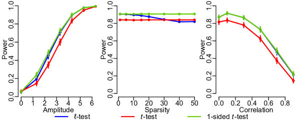
Figure 2: Power comparison of size-5$\%$ tests for $H_{j}$. For all the settings, we fix $n=100,d=50,\sigma=1$. For left, we fix $k=5,\bm{\Sigma}=\bm{I}$ and vary the amplitude $A$. For center, we fix $A=4.3,\bm{\Sigma}=\bm{I}$ and vary the sparsity level $k$. For right, we fix $A=4.3,k=5,\Sigma_{ij}=\rho^{|i-j|}$ and vary the inter-variable correlation $\rho$. The error bars represent plus or minus two standard errors.

The $\ell$-test significantly outperforms the $t$-test in sparse settings for any signal amplitude, achieving essentially one-sided $t$-test power for moderate-to-high signal amplitudes. The $\ell$-test’s power remains close to that of the one-sided $t$-test when as many as 30$\%$ of the coefficients are signals, and this phenomenon seems to be similar across covariate correlation levels. Furthermore, the $\ell$-test only starts to underperform the $t$-test after more than 60% of the coefficients are non-zero (as one might expect, given the $\ell$-test is designed to leverage sparsity), and even when the signal is fully dense (100% nonzero entries, all with equal magnitude), the $\ell$-test’s power loss is still only a fraction of its power gain in sparse settings.

5.2 Robustness of the $\ell$-test

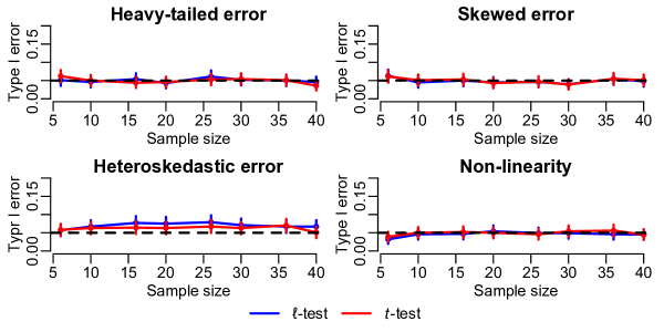
Figure 3: We vary the sample size ($n$) on the x-axis and set $d=n/2$. For the top-left, we draw $\epsilon_{i}\stackrel{{\scriptstyle i.i.d.}}{{\sim}}t_{2}$ (which does not have a finite second moment), for the top-right, $\epsilon_{i}\stackrel{{\scriptstyle i.i.d.}}{{\sim}}\mathrm{Exp}(1)$, standardized with its theoretical mean and standard deviation, and for the bottom-left, $\epsilon_{i}\stackrel{{\scriptstyle i.i.d.}}{{\sim}}N(0,1)$ if mean of the $i^{\mathrm{th}}$ row of $\bm{X}$ is less than the median of the row-means, while, $\epsilon_{i}\stackrel{{\scriptstyle i.i.d.}}{{\sim}}N(0,8)$, otherwise. For bottom-right, we generate $y_{i}\sim\mathcal{N}\left((\bm{X}_{i}^{4})^{T}\bm{\beta},\bm{I}\right)$, where, $(\bm{X}_{i}^{4})_{j}=X_{ij}^{4}$. All these settings use the nominal size of $5\%$ and the error bars represent plus or minus two units of standard error.

One thing that makes the $t$-test remarkable and so useful in practice is its robustness, even in relatively small samples, to violations of model (1.1). To evaluate the $\ell$-test’s robustness, we fix $d=n/2,k=1,\bm{\Sigma}=\bm{I}$, $A=3.3$, and test on a null index $\beta_{j}=0$. Figure 3 shows Type I error results for the $\ell$-test and $t$-test for four types of model violation: heavy-tailed errors, skewed errors, heteroskedastic errors, and model non-linearity (the figure caption gives exact specifications of each of the model violations) for a range of small sample sizes. In Appendix F.2 we present further simulations of these same four types of model violations, but Figure 3 shows the most extreme example of each of the four. Despite substantial deviations from (1.1), the $\ell$-test remains quite robust: like the $t$-test, it only makes even noticeable Type I error violations in the case of (very subtantial) heteroskedasticity, but even in this case (which is a well-known source of non-robustness for the $t$-test), the Type I error violation of the $\ell$-test remains close to that of the $t$-test and both are just a few percentage points above nominal.

5.3 Confidence Intervals for $\beta_{j}$

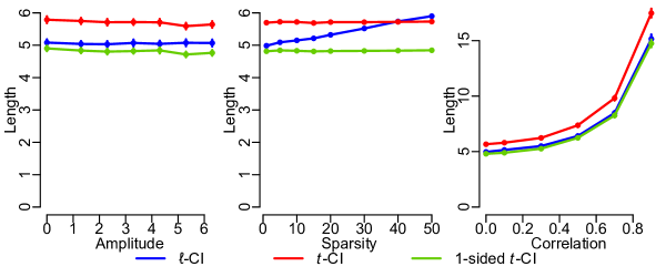
Figure 4: Coverage and lengths of the 95$\%$ confidence intervals. Figures on the left, center and right are under the exact same experimental settings as are the respective figures in Figure 2. The error bars represent plus or minus two standard errors.

We now perform simulations to compare the $\ell$-test confidence interval with the usual (two-sided) $t$-test confidence interval, as well as the interval obtained by inverting the one-sided $t$-test in the direction of the true sign of the alternative for every alternative $\beta_{j}=\gamma$. In Appendix G, we discuss an explicit characterization of this last interval, however a point we highlight here is that this is an oracle procedure (even more so than the one-sided $t$-test we compare to in Section 5.1) and can only be constructed if we know the exact true value of the coefficient, not just its sign. To obtain the $\ell$-test confidence interval, we choose a grid of candidate values for $\beta_{j}$ and report the coverage and length of the smallest interval that strictly encloses the rejected values of $\beta_{j}$ from both the ends. Note that this interval will always have length and coverage at least as large as the true $\ell$-test confidence interval (which we can never obtain exactly from a finite grid of $\beta_{j}$ values). We use brute force calculations using the highly optimized functions available in the package glmnet (Friedman et al., 2010) in R instead of our theoretically efficient algorithm in Appendix D for $\ell$-test inversion (and defer the task of designing an optimized implementation for it to future research).

For our simulations we consider the exact settings as in Figure 2 and summarize the results in Figure 4. We only report the lengths of all the intervals for a more compact presentation whereas the full results with empirical converges are reported in Appendix F.3 (the coverage is always extremely close to the nominal 95%). As expected, we see similar trends as in Figure 2, with the $\ell$-test confidence intervals being close to the oracle one-sided $t$-test intervals, consistently across amplitudes, in sparse settings. In the left and right plots, the $\ell$-test confidence intervals are consistently about $12\%$ shorter than their $t$-test based counterparts. Perhaps surprisingly, the center plot shows that the $\ell$-test’s benefit in confidence interval width over the $t$-test remains up until about 80% nonzero entries in the coefficient vector, which is a larger outperformance range of sparsity than in Figure 2. Similar to the power results, we see only a small detriment to using the $\ell$-test confidence interval in the densest setting, relative to its benefit in the sparsest setting. As with the power simulations, we also consider a setting with $d$ closer to $n$ in Appendix F.3, and again find this further narrows the gap between the $\ell$-test and one-sided $t$-test procedures.

5.4 Post-selection $\ell$-test inference

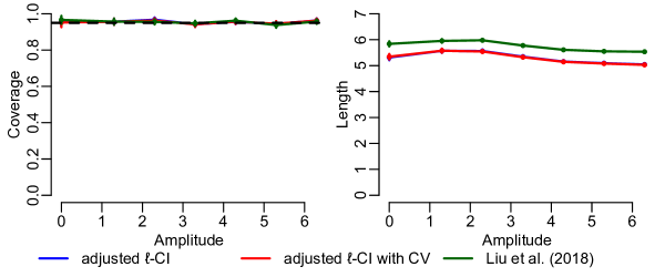
Figure 5: Length and coverage of various post-selection $95\%$ confidence intervals. We are under exactly the same setting as the left panel of Figure 4. Here ‘adjusted $\ell$-CI’ and ‘adjusted $\ell$-CI with CV’ refer to $\underline{\hat{C}}_{j}^{\lambda}$ and $\underline{\hat{C}}_{j}^{*\lambda}$, respectively, and we have used $\lambda=0.01$ (which approximately matched the average cross-validated value found on independent data sets, for the entire range of amplitudes). The error bars represent plus or minus two standard errors.

In this section, we perform simulations to empirically evaluate the performance of the adjusted $\ell$-test confidence intervals in Section 4 for post-selection inference in the linear model under LASSO selection. In particular, we will compare $\underline{\hat{C}}_{j}^{\lambda}$ and $\underline{\hat{C}}_{j}^{*\lambda}$, where for both of these methods we invert the respective adjusted $\ell$-tests on a grid of values using the same strategy as in Section 5.3, along with the conditional confidence interval procedure of Liu et al. (2018). Figure 5 shows the effect of varying coefficient amplitude on the length and coverage of the intervals (conditional on the LASSO selecting the coefficient) for the same setting as the left panels of Figures 2. We see there is practically no difference between the performance of $\underline{\hat{C}}_{j}^{\lambda}$ and $\underline{\hat{C}}_{j}^{*\lambda}$ (see figure caption for how $\lambda$ was chosen) and both are consistently shorter than the method in Liu et al. (2018), reflecting again the benefits of the $\ell$-test under sparsity but now conditional on LASSO selection. In Appendix F.4, we show results for an additional setting where $d$ is closer to $n$.

5.5 Analysis of the HIV drug resistance data

The HIV drug resistant data (Rhee et al., 2006) consists of 16 different regressions, each containing data on a set of genetic mutations (the covariates) and a score measuring resistance to an HIV drug (the response). We follow the same pre-processing step suggested in Barber and Candès (2015), resulting in 16 regressions with $n$ ranging between 328 and 842 and $d$ ranging between 147 and 313. Running the $t$-test on all covariates across all data sets results in an average power of 16.7%, while for the $\ell$-test it is 18.6% (this represents an 11% improvement), showing that the $\ell$-test’s theoretical benefits under sparsity provide genuine power gains in real data sets. Similarly, the $t$-test confidence intervals have an average width of 3.85 while the $\ell$-test confidence intervals’ is 3.54, representing about an 8% improvement. We also note that previous works studying the same data have aggregated discovered mutations to the gene level, and if we do this, the comparison remains similar: the $t$-test’s average power is 31.8% discovered genes while the $\ell$-test’s is 36.4% (a 14% improvement).

6 Discussion

The $\ell$-test leverages sparsity by using the LASSO coefficient estimate $|\hat{\beta}^{\lambda}_{j}|$ as its test statistic and can achieve power close to that of the one-sided $t$-test without any knowledge about the true sign of the coefficient. The $\ell$-test can be inverted to confidence intervals that are over 10% shorter than $t$-test intervals under sparsity, and the $\ell$-test and confidence intervals can also be adjusted for LASSO selection. A number of questions remain for future work:

1. A recentered $u_{1}$-based test. Section 2.2 argued that the $\ell$-test’s power gains under sparsity are derived from $\hat{m}_{j}$ tending to take the opposite sign of $\beta_{j}$, as this results in the $\ell$-test p-value (which uses the test statistic $|\hat{\beta}_{j}^{\lambda}|$) putting most of its weight on the “correct” tail of $\hat{\beta}_{j}^{\lambda}$. In fact, due to the increasing relationship between $u_{1}$ and $\hat{\beta}_{j}^{\lambda}$ established in Theorem 2.1, it is easy to see that a similar phenomenon occurs if we use $|u_{1}-\hat{m}_{j}|$ as the test statistic (note this is the same test statistic used to break ties in the $\ell$-test in Section 2.3), and indeed, although doing so produces a test that is numerically distinct from the $\ell$-test, the two tests perform very similarly. We presented the $\ell$-test in its current form because we expect it to be more interpretable for most (especially non-statistician) users to have its test statistic be a natural estimator of $\beta_{j}$ under sparsity, as well as because of the easy extension to post-selection inference, but recognizing that the test statistic $|u_{1}-\hat{m}_{j}|$ produces a very similar test may be helpful in generalizing the $\ell$-test idea or for theoretical study such as power analysis.

2. Extension to Gaussian means and, asymptotically, to general parametric models. A Gaussian means problem, wherein $\bm{w}\sim\mathcal{N}(\bm{\beta},\bm{\Sigma})$ is observed for some known positive-definite $\bm{\Sigma}$ (but $\bm{\beta}$ unknown), can always be converted to linear regression by taking $\bm{X}=\bm{\Sigma}^{-1/2}$ and $\bm{y}=\bm{\Sigma}^{-1/2}\bm{w}$, so that $\bm{y}\sim\mathcal{N}(\bm{X}\bm{\beta},\bm{I}_{n})$. The key point is that the $\ell$-test can be directly applied to any Gaussian means problem with known covariance matrix, with the analogous expectation that, when $\bm{\beta}$ is sparse, the $\ell$-test will outperform the standard $z$-test as long as $\bm{\Sigma}$ has sufficient off-diagonal entries (recall from Section 2.2 that the $\ell$-test’s power gain under sparsity derives from the sign-guessing ability of $\hat{m}_{j}$, which in turn relies on non-orthogonality of the columns of $\bm{X}$). This opens up many possible further applications of the $\ell$-test, including to any multivariate parametric model that admits an asymptotically multivariate Gaussian estimator and a consistent estimator for its covariance matrix, which includes both classical low-dimensional maximum likelihood or M-estimator asymptotics (see (Li and Fithian, 2021, Theorem 4) for an asymptotic result like this for knockoffs) as well as certain proportional asymptotic regimes with $n\propto d$ (Sur and Candès, 2019, Zhao et al., 2022).

3. Leveraging structure other than sparsity. The $\ell$-test leverages sparsity to improve upon the $t$-test, but it would be helpful to have analogous methods to use in settings that may not be sparse, but are believed to satisfy other forms of structure. For instance, if $\bm{\beta}$ is dense but smooth (i.e., it has small total variation), a test based on the fused LASSO (Tibshirani et al., 2005) may be more appropriate. The FAB method (Hoff, 2022) mentioned in Section 1.3 achieves a similar goal as the $\ell$-test for other forms of prior information and it may also be interesting to understand the relationship between the two.

Appendix A Characterization of the $\ell$-distribution under $H_{j}(\gamma):\beta_{j}=\gamma$

In Section 2.1, we characterized the conditional distribution, $\hat{\beta}_{j}^{\lambda}\mid\bm{S}^{(j)}$ under $H_{j}$ based on the quantiles of $u_{1}$. In this section, we extend the result to provide a similar characterization of the $\ell$-distribution under $H_{j}(\gamma):\beta_{j}=\gamma$.

Theorem A.1.

Consider the linear model defined in Theorem 2.1, fix $\gamma\in\mathbb{R}$ and define $\hat{\sigma}_{j}(\gamma)=\|(\bm{I}-\bm{P}_{-j})(\bm{y}-\gamma\bm{X}_{j})\|$. Then,

1. $\bm{S}^{(j)}(\gamma)=(\bm{X}_{-j}^{T}\bm{y},\|(\bm{I}-\bm{P}_{-j})(\bm{y}-\gamma\bm{X}_{j})\|)$ is sufficient under $H_{j}(\gamma)$. Furthermore, fixing an orthogonal matrix $\bm{V}$ for the column-space of $\bm{X}_{-j}$ as in Lemma 2.1, there exists a unique vector $\bm{u}^{\gamma}\in\mathbb{S}^{n-d}$ such that $\bm{y}=\hat{\bm{y}}_{j}+\gamma(\bm{I}-\bm{P}_{-j})\bm{X}_{j}+\hat{\sigma}_{j}(\gamma)\bm{V}\bm{u}^{\gamma}$ and

   $$\bm{u}^{\gamma}\mid\bm{S}^{(j)}(\gamma)\stackrel{{\scriptstyle H_{j}(\gamma)}}{{\sim}}\mathrm{Unif}\left(\mathbb{S}^{n-d}\right).$$

2. Furthermore, analogously define $\Lambda_{j}(\cdot,\cdot;\gamma):\mathbb{R}^{2}\mapsto\mathbb{R}$ by

   $$\Lambda_{j}(b,\epsilon;\gamma)=\frac{-\bm{X}_{j}^{T}(\hat{\bm{y}}_{j}+\gamma(\bm{I}-\bm{P}_{-j})\bm{X}_{j}-b\bm{X}_{j}-\bm{X}_{-j}\hat{\bm{\beta}}^{\lambda}_{-j}(b))+n\lambda\epsilon}{\hat{\sigma}_{j}(\gamma)\|(\bm{I}-\bm{P}_{-j})\bm{X}_{j}\|}.$$

   Then the function $f_{\bm{S}^{(j)}(\gamma)}^{\gamma}:\mathbb{R}\mapsto\mathbb{R}$, whose inverse is defined as

   $$\left(f_{\bm{S}^{(j)}(\gamma)}^{\gamma}\right)^{-1}(b)=\begin{cases}\Lambda_{j}(b,\mathrm{sign}(b);\gamma),&b\neq 0\\ [\Lambda_{j}(0,-1;\gamma),\Lambda_{j}(0,1;\gamma)],&b=0\end{cases},$$

   is continuous and increasing in $\mathbb{R}$ and strictly increasing in $\{u:f^{\gamma}_{\bm{S}^{(j)}(\gamma)}(u)\neq 0\}$ and satisfies $\hat{\beta}_{j}^{\lambda}=f^{\gamma}_{\bm{S}^{(j)}}(u^{\gamma}_{j})$.

Note that, as discussed in Section 4, the proof of item 1 of the above theorem directly follows from Lemma 2.1 applied to $(\bm{y}-\gamma\bm{X}_{j},\bm{X})$. Analogous to the proof of Theorem 2.1 using Lemma 2.1, one can derive item 2 of Theorem A.1 from its item 1, by defining $\bm{z}:=\bm{y}-\gamma\bm{X}_{j}$ and $\bm{\delta}$ by $\bm{\delta}_{-j}=\bm{\beta}_{-j}$ and $\delta_{j}=\beta_{j}-\gamma$ and copying exactly the same proof as in Appendix C.3 but by replacing $(\bm{y},\bm{\beta},\hat{\sigma}_{j})$ with $(\bm{z},\bm{\delta},\hat{\sigma}_{j}(\gamma))$ and then substituting back for $\bm{\delta}$ and $\bm{z}$ at the end. We thus skip an explicit proof of Theorem A.1.

Here we would also like to draw attention to the fact that the function $f_{\bm{S}^{(j)}(\gamma)}^{\gamma}$, for any $\gamma\in\mathbb{R}$, is defined for any real number $u$ and not necessarily restricted to $[0,1]$ and also that $\Lambda_{j}(b,\mathrm{sign}(b))$ can take values outside the $[-1,1]$ range. In fact if the values exceed this range, we can often draw conclusive insights about the behavior of the LASSO estimate $\hat{\beta}_{j}^{\lambda}$. For example, $\Lambda(0,\pm 1)<-1$ implies that $u_{1}^{\gamma}>\Lambda(0,1)$ and hence that for any $\bm{y}$ generated using the condition in Theorem A.1 for a $\bm{u}^{\gamma}\in\mathbb{S}^{n-d}$, the resultant LASSO estimator of the $j^{\mathrm{th}}$ coefficient, $\hat{\beta}_{j}^{\lambda}$, will always be positive. This can happen in situations as we next described in Section B and can in-fact, result in the $\ell$-test producing exactly the one-sided $t$-test p-value.

Appendix B Achieving the power of a one-sided $t$-test

The conclusions of the previous section show that if $\beta_{j}>0$ (which, without any loss of generality, we will assume throughout this section), the $\ell$-test would produce the exact p-value of a one-sided $t$-test if $\Lambda(0,\pm 1)=v_{\pm}<-1$ (as in this case $\hat{\beta}_{j}^{\lambda}>0$ under the null conditional distribution of $\bm{y}\mid\bm{S}^{(j)}$, and hence, the $\ell$-distribution puts all its mass on the positive half and we saw in Section 2 that the contribution from this part to the $\ell$-test p-value is exactly the one-sided $t$-test p-value). In this section, we will try to take a closer look at when this can be the case. Note that we introduced $\hat{m}_{j}$ in Section 2.2, defined by,

$$\hat{m}_{j}=\frac{-\bm{X}_{j}^{T}(\hat{\bm{y}}_{j}-\bm{X}_{-j}\hat{\bm{\beta}}^{\lambda}_{-j}(0))}{\hat{\sigma}_{j}\|(\bm{I}-\bm{P}_{-j})\bm{X}_{j}\|},$$

which is the mid-point of the interval $[v_{-},v_{+}]$, and argued that its numerator is a proxy to a quantity given by,

$$-\bm{X}_{j}^{T}(\bm{\hat{y}}_{j}-\bm{X}_{-j}\bm{\beta}_{-j})\sim\mathcal{N}(-\beta_{j}\bm{X}_{j}^{T}\bm{P}_{-j}\bm{X}_{j},\sigma^{2}\bm{X}_{j}^{T}\bm{P}_{-j}\bm{X}_{j}).$$

Thus roughly speaking, one can observe $v_{-},v_{+}\leq-1$ if $q_{j}=\frac{\beta_{j}\bm{X}_{j}^{T}\bm{P}_{-j}\bm{X}_{j}}{\|(\bm{I}-\bm{P}_{-j})\bm{X}_{j}\|}$ is highly positive. In particular, the magnitude of $q_{j}$ intuitively quantifies the reliability of the sign-guess. Notably, larger values of $|q_{j}|$ indicates higher differences between the mass the $\ell$-distribution assigns in the two halves of the real line (and hence is more asymmetric), thereby implying that the $\ell$-test p-value is much different from its two-sided-$t$-test counterpart. Now that we have an understanding of the role that $q_{j}$ plays, we next describe two situations in which one can observe $v_{-},v_{+}\leq-1$:

• Strong signal size: For any fixed design matrix $\bm{X}$, if the signal size $\beta_{j}$ is strong enough to make the quantity $q_{j}$ highly positive, one can expect that $\hat{m}_{j}$ would be sufficiently negative and hence, we can expect to see the p-value of a one-sided $t$-test. This result is intuitive as with increase in the signal size the variable gets more and more distinguishable. Thus the power of the one-sided $t$-test, the two-sided test and the $\ell$-test, all increase with the power of the latter getting closer to the power of the one-sided $t$-test.

• High feature correlation: Note that except for $\beta_{j}$, the other factor in $q_{j}$,

  $$\frac{\bm{X}_{j}^{T}\bm{P}_{-j}\bm{X}_{j}}{\|(\bm{I}-\bm{P}_{-j})\bm{X}_{j}\|}=\frac{\bm{X}_{j}^{T}\bm{P}_{-j}\bm{X}_{j}}{\sqrt{\|\bm{X}_{j}\|^{2}-\bm{X}_{j}^{T}\bm{P}_{-j}\bm{X}_{j}}},$$

  depends on the design. This shows that as $\bm{X}_{j}^{T}\bm{P}_{-j}\bm{X}_{j}$ increases and gets closer to $\bm{X}_{j}^{T}\bm{X}_{j}$, this factor starts blowing up and makes $q_{j}$ more positive highlighting another case when the power of the $\ell$-test can get closer to the power of the one-sided $t$-test. This, on the first glance, might seem non-intuitive because the increase in $\bm{X}_{j}^{T}\bm{P}_{-j}\bm{X}_{j}$ actually implies that the $j^{\mathrm{th}}$ variable gets more correlated with the rest of the variables and hence it should become harder to distinguish its effect. Note that unlike the previous case, in this case the power does not increase and as expected, the larger the quantity $\bm{X}_{j}^{T}\bm{P}_{-j}\bm{X}_{j}$ gets, the more the performance of all the three tests deteriorate. However with increase in $\bm{X}_{j}^{T}\bm{P}_{-j}\bm{X}_{j}$, the quantity $q_{j}$ increases in magnitude suggesting an increase in the belief about the validity of the sign guess. Put another way, with increase in $\bm{X}_{j}^{T}\bm{P}_{-j}\bm{X}_{j}$, it becomes possible to obtain a more reliable sign-guess as a function of the sufficient statistic, $\bm{S}^{(j)}$. Thus, though with this increasing correlation the tests loose power, the performances of the $\ell$-test and the one-sided $t$-test gets closer because of the improved sign-guessing ability of the former.

  Note that for design matrices, $\bm{X}$, of dimension $n\times d$ with i.i.d. drawn Gaussian columns (as is the case with most of the simulations in this paper), it indeed holds that with $d$ getting closer to $n$, the component $\bm{X}_{j}^{T}\bm{P}_{-j}\bm{X}_{j}$ increases in magnitude. Thus, in this case we would expect that the power curves of $\ell$-test and the one-sided $t$-test come closer as $d$ gets closer to $n$ (that is, as we move closer to un-identifiability).

Finally, note that it follows as a direct consequence of the discussions in this section and Section 2.2 that the $\ell$-test gains no power over the $t$-test if $\bm{X}_{j}$ is orthogonal with the rest of the columns (and in particular, for orthogonal designs). In this case, $\hat{m}_{j}=0$, so that we have no estimate of the sign of $\beta_{j}$ and hence, the $\ell$-distribution is symmetric about 0. With smoothing out of the p-value at $1$, we would expect the $\ell$-test and the $t$-test, as well as the respective confidence intervals, to perform similarly.

Appendix C Proofs

C.1 Proof of Lemma 2.1

Proof.

Because $\bm{V}$ is a full column-rank matrix, there exists a unique $\bm{u}$, such that,

$$\bm{V}\bm{u}=\frac{\bm{y}-\hat{\bm{y}}_{j}}{\|\bm{y}-\hat{\bm{y}}_{j}\|}=\frac{\bm{y}-\hat{\bm{y}}_{j}}{\hat{\sigma}_{j}}.$$

Clearly,

$$\|\bm{V}\bm{u}\|=\frac{\|\bm{y}-\hat{\bm{y}}_{j}\|}{\|\bm{y}-\hat{\bm{y}}_{j}\|}=1.$$

Because orthogonal transformations preserve norm, we must have that this unique $\bm{u}$ satisfy,

$$\|\bm{u}\|=\|\bm{V}\bm{u}\|=1,$$

which proves (2.1) in the statement of Lemma 2.1. The proof (2.2) follows directly from (Luo et al., 2022, Proposition E.1). $\square$

C.2 Proof of Lemma 2.2

Proof.

Note that we can write the OLS coefficient as (see (Fithian et al., 2014, Section 4)),

$$\hat{\beta}_{j,\mathrm{OLS}}=\frac{\bm{X}_{j}^{T}(\bm{I}-\bm{P}_{-j})\bm{y}}{\|(\bm{I}-\bm{P}_{-j})\bm{X}_{j}\|^{2}}.$$ (C.1)

We first start by showing that the OLS estimate, $\hat{\beta}_{j,\mathrm{OLS}}$, is a constant multiple of the statistic, $u_{1}$, where the constant is a deterministic function of the sufficient statistic, $\bm{S}^{(j)}$. Based on Lemma 2.1, we have the decomposition,

$$\bm{y}=\hat{\bm{y}_{j}}+\underbrace{\hat{\sigma}_{j}\bm{V}\bm{u}}_{\bm{\hat{}}e_{j}}.$$

This implies,

$$\begin{aligned} \bm{X}_{j}^{T}(\bm{I}-\bm{P}_{-j})\bm{y}&=\bm{X}_{j}^{T}(\bm{I}-\bm{P}_{-j})\bm{P}_{-j}\bm{y}+\hat{\sigma}_{j}\bm{X}_{j}^{T}(\bm{I}-\bm{P}_{-j})\bm{V}\bm{u}\\ &=\hat{\sigma}_{j}\bm{X}_{j}^{T}\bm{V}\bm{u}.\textrm{ [since the columns of }\bm{V}\textrm{ are orthogonal to the columns of }\bm{X}_{-j}]\end{aligned}$$ (C.2)

Note that from the choice of $\bm{V}$, we have that $\bm{V}_{1}=\frac{(\bm{I}-\bm{P}_{-j})\bm{X}_{j}}{\|(\bm{I}-\bm{P}_{-j})\bm{X}_{j}\|}$, and hence one can find other orthogonal vectors $\bm{v}_{i},i\in\{2,\dots,n-d+1\}$, such that, $\bm{V}=[\bm{v}_{1},\dots,\bm{v}_{n-d+1}]$. Then it follows that $\bm{X}_{j}^{T}\bm{v}_{i}=0,i>1$ and hence for $\bm{u}=(u_{1},\dots,u_{n-d+1})^{T}$,

$$\bm{X}_{j}^{T}\bm{V}\bm{u}=\bm{X}_{j}^{T}\sum_{i=1}^{n-d+1}\bm{v}_{i}u_{i}=\bm{X}_{j}^{T}\bm{V}_{1}u_{1}=\frac{\bm{X}_{j}^{T}(\bm{I}-\bm{P}_{-j})\bm{X}_{j}}{\|(\bm{I}-\bm{P}_{-j})\bm{X}_{j}\|}u_{1}=\|(\bm{I}-\bm{P}_{-j})\bm{X}_{j}\|u_{1},$$ (C.3)

thereby implying that,

$$\hat{\beta}_{j,\mathrm{OLS}}=\frac{\bm{X}_{j}^{T}(\bm{I}-\bm{P}_{-j})\hat{\bm{e}}_{j}}{\|(\bm{I}-\bm{P}_{-j})\bm{X}_{j}\|^{2}}.=\frac{\hat{\sigma}_{j}u_{1}}{\|(\bm{I}-\bm{P}_{-j})\bm{X}_{j}\|}$$ (C.4)

Note that the factor pre-multiplying $u_{1}$ in the above equation is a function of the sufficient statistic, $\bm{S}^{(j)}$, and the design matrix, $\bm{X}$. Thus for samples from $\bm{y}\mid\bm{S}^{(j)}$, under $H_{j}$, showing that a statistic is increasing in $u_{1}$ or $\hat{\beta}_{j,\mathrm{OLS}}$ are equivalent.

Next, we show that the $t$-test statistic is an increasing function of $\hat{\beta}_{j,\mathrm{OLS}}$. For that, we first decompose the error term $\hat{\bm{e}}_{j}$ as $\hat{\bm{e}}_{j}=\hat{\bm{e}}_{\parallel}+\hat{\bm{e}}_{\perp}$, where,

$$\begin{aligned} &\hat{\bm{e}}_{\parallel}=\frac{(\bm{I}-\bm{P}_{-j})\bm{X}_{j}\bm{X}_{j}^{T}(\bm{I}-\bm{P}_{-j})\hat{\bm{e}}_{j}}{\|(\bm{I}-\bm{P}_{-j})\bm{X}_{j}\|^{2}}=(\bm{I}-\bm{P}_{-j})\bm{X}_{j}\hat{\beta}_{j,\mathrm{OLS}}\textrm{, and }\\ &\hat{\bm{e}}_{\perp}=\left(\bm{I}-\frac{(\bm{I}-\bm{P}_{-j})\bm{X}_{j}\bm{X}_{j}^{T}(\bm{I}-\bm{P}_{-j})}{\|(\bm{I}-\bm{P}_{-j})\bm{X}_{j}\|^{2}}\right)\hat{\bm{e}}_{j}.\end{aligned}$$ (C.5)

Note that $\hat{\bm{e}}_{\parallel}$ is the component of $\hat{\bm{e}}_{j}$ along the component of $\bm{X}_{j}$ orthogonal to $\bm{X}_{-j}$, while the component $\hat{\bm{e}}_{\perp}$ is perpendicular to the columnspace of the entire $\bm{X}$. Furthermore, the components, $\hat{\bm{e}}_{\perp}$ and $\hat{\bm{e}}_{\parallel}$ are themselves orthogonal to each other. Using the relation $\hat{\bm{e}}_{j}=\hat{\sigma}_{j}\bm{V}\bm{u}$ and the fact that the matrix pre-multiplying $\hat{\bm{e}}_{j}$ to obtain $\hat{\bm{e}}_{\perp}$ is idempotent, one can write,

$$\|\hat{\bm{e}}_{\perp}\|^{2} =\hat{\sigma}_{j}^{2}\bm{u}^{T}\bm{V}^{T}\left(\bm{I}-\frac{(\bm{I}-\bm{P}_{-j})\bm{X}_{j}\bm{X}_{j}^{T}(\bm{I}-\bm{P}_{-j})}{\|(\bm{I}-\bm{P}_{-j})\bm{X}_{j}\|^{2}}\right)\bm{V}\bm{u}$$

$$=\hat{\sigma}_{j}^{2}\bm{u}^{T}\bm{V}^{T}\bm{V}\bm{u}-\frac{\left(\bm{X}_{j}^{T}\hat{\bm{e}}_{j}\right)^{2}}{\|(\bm{I}-\bm{P}_{-j})\bm{X}_{j}\|^{2}}$$

$$=\hat{\sigma}_{j}^{2}-\frac{\left(\bm{X}_{j}^{T}\hat{\bm{e}}_{j}\right)^{2}}{\|(\bm{I}-\bm{P}_{-j})\bm{X}_{j}\|^{2}}\textrm{ }\left[\because\bm{V}\textrm{ is an orthogonal matrix and }\bm{u}^{T}\bm{u}=1\right]$$

$$=\hat{\sigma}_{j}^{2}-\left(\hat{\beta}_{j,\mathrm{OLS}}\right)^{2}\|(\bm{I}-\bm{P}_{-j})\bm{X}_{j}\|^{2}$$

Because $\hat{\bm{e}}_{\perp}$ is in the orthogonal complement of the columnspace of $\bm{X}$, we can write,

$$(\bm{I}-\bm{P})\hat{\bm{e}}_{j}=\hat{\bm{e}}_{\perp}+(\bm{I}-\bm{P})\hat{\bm{e}}_{\parallel}.$$

Also,

$$\|(\bm{I}-\bm{P})\hat{\bm{e}}_{j}\|^{2} =\|\hat{\bm{e}}_{\perp}\|^{2}+\|(\bm{I}-\bm{P})\hat{\bm{e}}_{\parallel}\|^{2}$$

$$=\hat{\sigma}_{j}^{2}-\left(\hat{\beta}_{j,\mathrm{OLS}}\right)^{2}\|(\bm{I}-\bm{P}_{-j})\bm{X}_{j}\|^{2}+\|(\bm{I}-\bm{P})(\bm{I}-\bm{P}_{-j})\bm{X}_{j}\|^{2}(\hat{\beta}_{j,\mathrm{OLS}})^{2}$$

$$=\hat{\sigma}_{j}^{2}-(\hat{\beta}_{j,\mathrm{OLS}})^{2}\left(\|(\bm{I}-\bm{P}_{-j})\bm{X}_{j}\|^{2}-\|(\bm{I}-\bm{P})(\bm{I}-\bm{P}_{-j})\bm{X}_{j}\|^{2}\right)$$

$$=\hat{\sigma}_{j}^{2}-(\hat{\beta}_{j,\mathrm{OLS}})^{2}\underbrace{\|\bm{P}(\bm{I}-\bm{P}_{-j})\bm{X}_{j}\|^{2}}_{=:\,\kappa}.$$

With these expressions, we can write,

$$T_{j}=\frac{\hat{\beta}_{j,OLS}}{\hat{\sigma}\sqrt{(\bm{X}^{T}\bm{X})^{-1}_{j,j}}}=C\frac{\hat{\beta}_{j,\mathrm{OLS}}}{\sqrt{\hat{\sigma}_{j}^{2}-\left(\hat{\beta}_{j,\mathrm{OLS}}\right)^{2}\kappa}}=C\frac{\frac{\hat{\sigma}_{j}u_{1}}{\|(\bm{I}-\bm{P}_{-j})\bm{X}_{j}\|}}{\sqrt{\hat{\sigma}_{j}^{2}-u_{1}^{2}\left(\frac{\hat{\sigma}_{j}}{\|(\bm{I}-\bm{P}_{-j})\bm{X}_{j}\|}\right)^{2}\kappa}},$$

where, $C=\sqrt{\frac{n-d}{(\bm{X}^{T}\bm{X})^{-1}_{j,j}}}$ and $\kappa$ are both positive. Defining, $C^{\prime}=C\cdot\frac{\hat{\sigma}_{j}}{\|(\bm{I}-\bm{P}_{-j})\bm{X}_{j}\|}$, $\kappa^{\prime}=\kappa\cdot\left(\frac{\hat{\sigma}_{j}}{\|(\bm{I}-\bm{P}_{-j})\bm{X}_{j}\|}\right)^{2}$ and $g_{\bm{S}^{(j)}}(u)=\frac{C^{\prime}u}{\sqrt{\hat{\sigma}_{j}^{2}-u^{2}\kappa^{\prime}}}$, the above equation shows $T_{j}=g_{\bm{S}^{(j)}}(u_{1})$, thereby establishing that, $g_{\bm{S}^{(j)}}$ is a functional of $\bm{S}^{(j)}$ and itself is continuous, strictly increasing and anti-symmetric. $\square$

C.3 Proof of Theorem 2.1

We will first prove that $f_{\bm{S}^{(j)}}$ is continuous and strictly increasing in $\{u:f_{\bm{S}^{(j)}}(u)\neq 0\}$ (in C.3.1), followed by a proof of the characterization of its inverse (in C.3.2).

C.3.1 Proof of continuity and increasing properties of $f_{\mathbf{S}_{j}}$

In this section, we will prove that $f_{\bm{S}^{(j)}}$ is continuous and strictly increasing in $\{u:f_{\bm{S}^{(j)}}(u)\neq 0\}$.

Proof.

We again start with the decomposition,

$$\bm{y}=\hat{\bm{y}}_{j}+\underbrace{\hat{\sigma}_{j}\bm{V}\bm{u}}_{\hat{\bm{e}}_{j}},$$

and as we did in the proof in Section C.2, we again decompose,

$$\hat{\bm{e}}_{j}=\hat{\bm{e}}_{||}+\hat{\bm{e}}_{\perp}.$$

Next using Equation (C.1) and (C.4),

$$u_{1}=\frac{\bm{X}_{j}^{T}(\bm{I}-\bm{P}_{-j})\bm{y}}{\hat{\sigma}_{j}\|(\bm{I}-\bm{P}_{-j})\bm{X}_{j}\|}=\frac{\bm{X}_{j}^{T}(\bm{I}-\bm{P}_{-j})\hat{\bm{e}}_{j}}{\hat{\sigma}_{j}\|(\bm{I}-\bm{P}_{-j})\bm{X}_{j}\|}.$$

Also from Equation (C.5),

$$\hat{\bm{e}}_{\parallel}=\frac{(\bm{I}-\bm{P}_{-j})\bm{X}_{j}\bm{X}_{j}^{T}(\bm{I}-\bm{P}_{-j})\hat{\bm{e}}_{j}}{\|(\bm{I}-\bm{P}_{-j})\bm{X}_{j}\|^{2}}=\frac{\hat{\sigma}_{j}(\bm{I}-\bm{P}_{-j})\bm{X}_{j}u_{1}}{\|(\bm{I}-\bm{P}_{-j})\bm{X}_{j}\|}.$$

Based on these relations, we have,

$$\begin{aligned} &\|\bm{y}-\bm{X}\bm{\beta}\|^{2}+2n\lambda|\beta_{j}|+2n\lambda\sum_{i\neq j}|\beta_{i}|\\ &=\|\hat{\bm{y}}_{j}+\hat{\bm{e}}_{j}-\bm{X}_{-j}\bm{\beta}_{-j}-\bm{X}_{j}\beta_{j}\|^{2}+2n\lambda|\beta_{j}|+2n\lambda\sum_{i\neq j}|\beta_{i}|\\ &=\|\hat{\bm{y}}_{j}-\bm{X}_{-j}\bm{\beta}_{-j}-\bm{P}_{-j}\bm{X}_{j}\beta_{j}+\hat{\bm{e}}_{j}-(\bm{I}-\bm{P}_{-j})\bm{X}_{j}\beta_{j}\|^{2}+2n\lambda|\beta_{j}|+2n\lambda\sum_{i\neq j}|\beta_{i}|\\ &=\|\hat{\bm{y}}_{j}-\bm{X}_{-j}\bm{\beta}_{-j}-\bm{P}_{-j}\bm{X}_{j}\beta_{j}+\hat{\bm{e}}_{\perp}+\hat{\bm{e}}_{\parallel}-(\bm{I}-\bm{P}_{-j})\bm{X}_{j}\beta_{j}\|^{2}\\ &+2n\lambda|\beta_{j}|+2n\lambda\sum_{i\neq j}|\beta_{i}|\textrm{ [}\hat{\bm{e}}_{\perp},\hat{\bm{e}}_{\parallel}\textrm{ are defined above]}\\ &=\|\hat{\bm{y}}_{j}-\bm{X}_{-j}\bm{\beta}_{-j}-\bm{P}_{-j}\bm{X}_{j}\beta_{j}\|^{2}+\|\hat{\bm{e}}_{\perp}\|^{2}+\|\hat{\bm{e}}_{\parallel}-(\bm{I}-\bm{P}_{-j})\bm{X}_{j}\beta_{j}\|^{2}+2n\lambda|\beta_{j}|+2n\lambda\sum_{i\neq j}|\beta_{i}|\\ &=\|\hat{\bm{y}}_{j}-\bm{X}_{-j}\bm{\beta}_{-j}-\bm{P}_{-j}\bm{X}_{j}\beta_{j}\|^{2}+\|\hat{\bm{e}}_{\perp}\|^{2}+\left(\frac{u_{1}\hat{\sigma}_{j}}{\|(\bm{I}-\bm{P}_{-j})\bm{X}_{j}\|}-\beta_{j}\right)^{2}\|(\bm{I}-\bm{P}_{-j})\bm{X}_{j}\|^{2}\\ &+2n\lambda|\beta_{j}|+2n\lambda\sum_{i\neq j}|\beta_{i}|\\ &=\tilde{f}(\bm{\beta};\bm{y},\bm{X})+\left(\frac{u_{1}\hat{\sigma}_{j}}{\|(\bm{I}-\bm{P}_{-j})\bm{X}_{j}\|}-\beta_{j}\right)^{2}\|(\bm{I}-\bm{P}_{-j})\bm{X}_{j}\|^{2},\end{aligned}$$ (C.6)

$\tilde{f}(\bm{\beta};\bm{y},\bm{X})$ denotes the expression it is replacing, and whenever the context is clear, we will use $\tilde{f}$ to denote $\tilde{f}(\bm{\beta};\bm{y},\bm{X})$. Note that $\tilde{f}$ also depends on $\lambda>0$, but for compactness, we have suppressed this in the notation as in the following lines we will not be interested in the behavior of $\tilde{f}$ as a function of $\lambda$. In fact, we will only analyze $\tilde{f}$ as a function of the argument $\bm{\beta}$. Thus we have,

$$\underset{\bm{\beta}}{\arg\min}\left(\|\bm{y}-\bm{X}\bm{\beta}\|^{2}+2n\lambda|\beta_{j}|+2n\lambda\sum_{i\neq j}|\beta_{i}|\right)$$

$$=\underset{\bm{\beta}}{\arg\min}\left(\tilde{f}+\left(\frac{\hat{\sigma}_{j}u_{1}}{\|(\bm{I}-\bm{P}_{-j})\bm{X}_{j}\|}-\beta_{j}\right)^{2}\|(\bm{I}-\bm{P}_{-j})\bm{X}_{j}\|^{2}\right).$$

Define

$$\hat{\bm{\beta}}(a):=\underset{\bm{\beta}}{\arg\min}\left(\underbrace{\tilde{f}+\left(a-\beta_{j}\right)^{2}\|(\bm{I}-\bm{P}_{-j})\bm{X}_{j}\|^{2}}_{=:U(a,\bm{\beta};\bm{y},\bm{X})}\right).$$ (C.7)

Thus, $\hat{\beta}_{j}\left(\frac{\hat{\beta}_{j,\mathrm{OLS}}}{\|(\bm{I}-\bm{P}_{-j})\bm{X}_{j}\|^{2}}\right)$ is just the LASSO estimate of $\beta_{j}$, $\hat{\beta}^{\lambda}_{j}$ and hence, it suffices to show that $\hat{\beta}^{\lambda}_{j}(a)$ is a non-decreasing function of $a$. As is the case with the function, $\tilde{f}$, we will also be primarily be interested in the behavior of $U$ as a function of the arguments, $(a,\bm{\beta})$. We start with listing some properties of the function, $U$. First, note that $U$ is a continuous, convex function in its arguments and is strictly convex in $a$ for any fixed value of $\bm{\beta}$. This implies that $\hat{\bm{\beta}}(a)$ is continuous in $a$. To see this, first note that as $\|\bm{\beta}\|\rightarrow\infty$, the function, $U$ diverges, so that for the minimization problem to obtain $\hat{\bm{\beta}}(a)$, we can constraint $\bm{\beta}$ within some compact set, $C(a)\subset\mathbb{R}^{d}$. One can then apply Berge’s Maximum Theorem (Berge, 1963), to conclude that $\hat{\bm{\beta}}(a)$ is continuous in $a$.

Next, note that the only non-differentiable component in the expression of $U$ is the $\ell_{1}$-penalty of $\bm{\beta}$, which implies that the $U$ has a partial derivative in $\beta_{j}$ at all non-zero values of $\beta_{j}$. Consider a value of $a$ such that $\hat{\beta}_{j}(a)\neq 0$ and let $\mathcal{A}(a)=\{i\in[1:k]\setminus\{j\}:\hat{\beta}_{i}(a)\neq 0\}$ denote the active set among the remaining variables.

Note that because $\hat{\bm{\beta}}(a)$ maximizes $U$, and $\forall i\notin\mathcal{A}(a)\cup\{j\}$, $\hat{\bm{\beta}}_{j}(a)=0$, it holds that $\hat{\bm{\beta}}_{\mathcal{A}(a)\cup\{j\}}(a)$ is a minimizer of $U(a,\bm{\gamma};\bm{y},\bm{X}_{\mathcal{A}(a)\cup\{j\}})$, where now $\bm{\gamma}$ is a vector of length $|\mathcal{A}(a)\cup\{j\}|$. For a proof, see Lemma 1 of (Liu et al., 2021+, Section 3.2). Because all the entries of $\hat{\bm{\beta}}_{\mathcal{A}(a)\cup\{j\}}$ are non-zero, $U(a,\bm{\gamma};\bm{y},\bm{X}_{\mathcal{A}(a)\cup\{j\}})$ is differentiable in $\bm{\gamma}$ at $\hat{\bm{\beta}}_{\mathcal{A}(a)\cup\{j\}}$, and because the latter is a minimizer, an appeal to the first-order stationary conditions yield that for any $i\in\mathcal{A}(a)$,

$$\frac{\partial}{\partial\gamma_{i}}U(a,\bm{\gamma};\bm{y},\bm{X}_{\mathcal{A}(a)\cup\{j\}})\big{|}_{\bm{\gamma}=\hat{\bm{\beta}}_{\mathcal{A}(a)\cup\{j\}}}(a)=0$$

$$\implies -\bm{X}_{i}^{T}(\hat{\bm{y}}_{j}-\bm{X}_{\mathcal{A}(a)}\hat{\bm{\beta}}_{\mathcal{A}(a)}(a)-\bm{P}_{-j}\bm{X}_{j}\hat{\beta}^{\lambda}_{j}(a))+2n\lambda\mathrm{sign}(\hat{\beta}_{i}(a))=0$$

Note that from the continuity of $\hat{\bm{\beta}}(a)$ in the neighbourhood of $a$ where $\mathcal{A}(a)$ does not change, the sign of the active variables also remain constant so that $\mathrm{sign}(\hat{\beta}_{i}(a))$ is a constant in that neighborhood, $\forall i\in\mathcal{A}(a)\cup\{j\}$. Thus, differentiating the above equation both the sides with respect to $a$ yields,

$$\bm{X}_{i}^{T}\bm{X}_{\mathcal{A}(a)}\frac{\partial}{\partial a}\hat{\bm{\beta}}_{\mathcal{A}(a)}+\bm{X}_{i}^{T}\bm{P}_{-j}\bm{X}_{j}\frac{\partial}{\partial a}\hat{\beta}_{j}(a)=0,\forall i\in\mathcal{A}(a)$$

$$\implies \bm{X}_{\mathcal{A}(a)}^{T}\bm{X}_{\mathcal{A}(a)}\frac{\partial}{\partial a}\hat{\bm{\beta}}_{\mathcal{A}(a)}+\bm{X}_{\mathcal{A}(a)}^{T}\bm{P}_{-j}\bm{X}_{j}\frac{\partial}{\partial a}\hat{\beta}_{j}(a)=\bm{0}$$

$$\implies \frac{\partial}{\partial a}\hat{\bm{\beta}}_{\mathcal{A}(a)}=-\left(\bm{X}_{\mathcal{A}(a)}^{T}\bm{X}_{\mathcal{A}(a)}\right)^{-1}\bm{X}_{\mathcal{A}(a)}^{T}\bm{P}_{-j}\bm{X}_{j}\frac{\partial}{\partial a}\hat{\beta}_{j}(a)$$

Similarly using the first-order stationary condition on the index $j$ yields,

$$-\bm{X}_{j}^{T}\bm{P}_{-j}(\hat{\bm{y}}_{j}-\bm{X}_{\mathcal{A}(a)}\hat{\bm{\beta}}_{\mathcal{A}(a)}(a)-\bm{P}_{-j}\bm{X}_{j}\hat{\beta}^{\lambda}_{j}(a))-(a-\hat{\beta}^{\lambda}_{j}(a))\|(\bm{I}-\bm{P}_{-j})\bm{X}_{j}\|^{2}=0$$

$$\implies \bm{X}_{j}^{T}\bm{X}_{\mathcal{A}(a)}\frac{\partial}{\partial a}\hat{\bm{\beta}}_{\mathcal{A}(a)}(a)+\bm{X}_{j}^{T}\bm{P}_{-j}\bm{X}_{j}\frac{\partial}{\partial a}\hat{\beta}^{\lambda}_{j}(a)-\left(1-\frac{\partial}{\partial a}\hat{\beta}^{\lambda}_{j}(a)\right)\|(\bm{I}-\bm{P}_{-j})(\bm{X}_{j})\|^{2}=0$$

$$\implies -\bm{X}_{j}^{T}\bm{X}_{\mathcal{A}(a)}\left(\bm{X}_{\mathcal{A}(a)}^{T}\bm{X}_{\mathcal{A}(a)}\right)^{-1}\bm{X}_{\mathcal{A}(a)}^{T}\bm{P}_{-j}\bm{X}_{j}\frac{\partial}{\partial a}\hat{\beta}_{j}(a)+\bm{X}_{j}^{T}\bm{X}_{j}\frac{\partial}{\partial a}\hat{\beta}^{\lambda}_{j}(a)=\|(\bm{I}-\bm{P}_{-j})(\bm{X}_{j})\|^{2}$$

$$\implies -\bm{X}_{j}^{T}\bm{P}_{\mathcal{A}(a)}\bm{P}_{-j}\bm{X}_{j}\frac{\partial}{\partial a}\hat{\beta}_{j}(a)+\|\bm{X}_{j}\|^{2}\frac{\partial}{\partial a}\hat{\beta}^{\lambda}_{j}(a)=\|(\bm{I}-\bm{P}_{-j})(\bm{X}_{j})\|^{2}$$

$$\implies -\bm{X}_{j}^{T}\bm{P}_{\mathcal{A}(a)}\bm{X}_{j}\frac{\partial}{\partial a}\hat{\beta}_{j}(a)+\|\bm{X}_{j}\|^{2}\frac{\partial}{\partial a}\hat{\beta}^{\lambda}_{j}(a)=\|(\bm{I}-\bm{P}_{-j})(\bm{X}_{j})\|^{2}$$

$$\implies \frac{\partial}{\partial a}\hat{\beta}^{\lambda}_{j}(a)=\frac{\|(\bm{I}-\bm{P}_{-j})(\bm{X}_{j})\|^{2}}{\|\bm{X}_{j}\|^{2}-\|\bm{P}_{\mathcal{A}(a)}\bm{X}_{j}\|^{2}}=\frac{\|(\bm{I}-\bm{P}_{-j})(\bm{X}_{j})\|^{2}}{\|(\bm{I}-\bm{P}_{\mathcal{A}(a)})(\bm{X}_{j})\|^{2}},$$

which is positive, whenever $\hat{\beta}^{\lambda}_{j}(a)\neq 0$. Hence, for an $a\in\mathbb{R}$, either $\hat{\beta}^{\lambda}_{j}(a)=0$ or $\frac{\partial\hat{\beta}_{j}(a)}{\partial a}>0$, showing that $\hat{\beta}^{\lambda}_{j}$ is locally increasing around $a$ in the latter case. Now define,

$$f_{\bm{S}^{(j)}}(u)=\hat{\beta}_{j}^{\lambda}\left(u\cdot\frac{\hat{\sigma}_{j}}{\|(\bm{I}-\bm{P}_{-j})\bm{X}_{j}\|}\right),$$

and note that, $\hat{\beta}_{j}^{\lambda}=f_{\bm{S}^{(j)}}(u_{1})$. Furthermore, note that $f_{\bm{S}^{(j)}}$ is a functional of the sufficient statistic, $\bm{S}^{(j)}$, and using the arguments above, is a continuous, piece-wise linear function that is increasing in the region, $\{u:f_{\bm{S}^{(j)}}(u)\neq 0\}$. This establishes all the claims about $f_{\bm{S}^{(j)}}$ in the statement of Theorem 2.1 except for (2.4), which we turn to next.

$\square$

C.3.2 Proof of Equation (2.4) in Theorem 2.1

To prove Equation (2.4), we first start with an intermediate result.

Theorem C.1.

For data $(\bm{y},\bm{X})$, with $\bm{X}$ full column-rank and $\lambda>0$, define $\bm{\hat{\beta}}_{*}^{\lambda}(b)$ to be $b$ at the $j^{\mathrm{th}}$ coordinate and $\bm{\hat{\beta}}_{-j}^{\lambda}(b)$ on the rest, where, $\bm{\hat{\beta}}_{-j}^{\lambda}(b)$ is defined as in Equation (2.3). Also let

$$f_{\lambda}(\bm{y};\bm{\beta}):=\frac{1}{2n}\|\bm{y}-\bm{X}\bm{\beta}\|^{2}+\lambda\|\bm{\beta}\|_{1},$$ (C.8)

be the LASSO objective function. Then for any $b\in\mathbb{R}$, the following are equivalent

1. $0\in\partial_{\beta_{j}}f_{\lambda}({\bm{y}};{\bm{\beta}})\big{\lvert}_{\bm{\beta}=\hat{\bm{\beta}}_{*}^{\lambda}(b)}$

2. $\hat{\bm{\beta}}^{\lambda}=\hat{\bm{\beta}}_{*}^{\lambda}(b)$

3. $\hat{\beta}_{j}^{\lambda}=b$

Proof of Theorem C.1.

We first show the equivalence of (a) and (b). Assume that, $0\in\partial_{\beta_{j}}f_{\lambda}({\bm{y}};{\bm{\beta}})\big{\lvert}_{\bm{\beta}=\hat{\bm{\beta}}_{*}^{\lambda}(b)}$. The convexity of $f_{\lambda}({\bm{y}};(\bm{\beta}_{-j}=\hat{\bm{\beta}}_{-j}^{\lambda}(b),\beta_{j}))$ in $\beta_{j}$ shows that the $j^{\mathrm{th}}$ entry of $\hat{\bm{\beta}}_{*}^{\lambda}(b)$ is the minimizer of $f_{\lambda}({\bm{y}};(\bm{\beta}_{-j}=\bm{\hat{}}{\bm{\beta}}_{-j}^{\lambda}(b),\beta_{j}))$ in $\beta_{j}$. That is,

$$\underset{\beta_{j}}{\arg\min}f_{\lambda}({\bm{y}};(\bm{\beta}_{-j}=\hat{\bm{\beta}}_{-j}^{\lambda}(b),\beta_{j}))=b.$$

But by the definition of $\hat{\bm{\beta}}^{\lambda}_{-j}(b)$, we know that

$$\underset{\bm{\beta}_{-j}}{\arg\min}f_{\lambda}({\bm{y}};(\bm{\beta}_{-j},\beta_{j}=b))=\hat{\bm{\beta}}_{-j}^{\lambda}(b).$$

Thus, if one runs a blockwise coordinate descent with blocks $\{j\}$ and $[1:p]\setminus\{j\}$ starting at $\hat{\bm{\beta}}_{*}^{\lambda}(b)$, we see that the iterates will be constant at $\hat{\bm{\beta}}_{*}^{\lambda}(b)$, thereby implying that this is a limit point of the iterates. One can now invoke (Tseng, 2001, Proposition 5.1) (the conditions for applying this proposition follow directly as $f_{\lambda}$ can be separated into the squared error loss and the non-differentiable $\ell_{1}$-penalty) to conclude that,

$$\hat{\bm{\beta}}=\underset{\bm{\beta}}{\arg\min}f_{\lambda}({\bm{y}};\bm{\beta})=\hat{\bm{\beta}}_{*}^{\lambda}(b),$$

which establishes the implication of (a) to (b). The reverse implication follows directly from the fact that $\hat{\bm{\beta}}$ is the optimizer of the LASSO objective, so that each coordinate, and in particular the $j^{\mathrm{th}}$ coordinate of the sub-gradient, contains 0, that is, $0\in\partial_{\beta_{j}}f_{\lambda}({\bm{y}};{\bm{\beta}})\big{\lvert}_{\bm{\beta}=\hat{\bm{\beta}}}$. The fact that $\hat{\bm{\beta}}=\hat{\bm{\beta}}_{*}^{\lambda}(b)$ completes the argument. It is also straightforward to see that (b) implies (c). To show that (c) implies (b), note that one can use the blockwise coordinate descent argument used above to conclude that $\hat{\bm{\beta}}^{\lambda}=\hat{\bm{\beta}}^{\lambda}(\hat{\beta}_{j}^{\lambda})$, and then use the hypothesis of (c) (that is, $\hat{\beta}_{j}^{\lambda}=b$) to conclude (b). $\square$

Hence, Theorem C.1 now implies that $\hat{\beta}_{j}^{\lambda}=b$ if and only if $0\in\partial_{\beta_{j}}f_{\lambda}(\bm{y};\bm{\beta})\lvert_{\bm{\beta}=\hat{\bm{\beta}}_{*}^{\lambda}(b)}$. We will now prove item 2 of Theorem 2.1 by evaluating this sub-gradient.

Proof of item 2 of Theorem 2.1.

Note that we have the following decomposition,

$$f_{\lambda}({\bm{y}};\bm{\beta})$$

$$=\frac{1}{2n}\|{\bm{y}}-\bm{X}\bm{\beta}\|^{2}+\lambda\|\bm{\beta}\|_{1}$$

$$=\frac{1}{2n}\|\hat{\bm{y}}_{j}+\hat{\sigma}_{j}\bm{V}\bm{u}-\bm{P}_{-j}\bm{X}_{j}\beta_{j}-(\bm{I}-\bm{P}_{-j})\bm{X}_{j}\beta_{j}-\bm{X}_{-j}\bm{\beta}_{-j}\|^{2}+\lambda\|\bm{\beta}\|_{1}$$

$$=\frac{1}{2n}\|\hat{\bm{y}}_{j}-\bm{P}_{-j}\bm{X}_{j}\beta_{j}-\bm{X}_{-j}\bm{\beta}_{-j}\|^{2}+\frac{1}{2n}\|\hat{\sigma}_{j}\bm{V}\bm{u}-(\bm{I}-\bm{P}_{-j})\bm{X}_{j}\beta_{j}\|+\lambda|\beta_{j}|+\lambda\sum_{i\neq j}|\beta_{i}|$$

Now define,

$$s(\beta_{j})=\begin{cases}[-1,1],&\beta_{j}=0\\ \mathrm{sign}(\beta_{j}),&\beta_{j}\neq 0\end{cases}.$$

Then we have,

$$\partial_{\beta_{j}}f_{\lambda}({\bm{y}};\bm{\beta})$$

$$=-\frac{1}{n}\bm{X}_{j}^{T}\bm{P}_{-j}(\hat{\bm{y}}_{j}-\bm{P}_{-j}\bm{X}_{j}\beta_{j}-\bm{X}_{-j}\bm{\beta}_{-j})-\frac{1}{n}\bm{X}_{j}^{T}(\bm{I}-\bm{P}_{-j})\left(\hat{\sigma}_{j}\bm{V}\bm{u}-(\bm{I}-\bm{P}_{-j})\bm{X}_{j}\beta_{j}\right)+\lambda s(\beta_{j})$$

$$=-\frac{1}{n}\bm{X}_{j}^{T}\hat{\bm{y}}_{j}-\frac{\hat{\sigma}_{j}}{n}\bm{X}_{j}^{T}\bm{V}\bm{u}+\frac{\bm{X}_{j}^{T}\bm{P}_{-j}\bm{X}_{j}\beta_{j}+\bm{X}_{j}^{T}(\bm{I}-\bm{P}_{-j})\bm{X}_{j}\beta_{j}+\bm{X}_{j}^{T}\bm{X}_{-j}\bm{\beta}_{-j}}{n}+\lambda s(\beta_{j})$$

$$=-\frac{1}{n}\bm{X}_{j}^{T}\hat{\bm{y}}_{j}-\frac{\hat{\sigma}_{j}}{n}\bm{X}_{j}^{T}\bm{V}\bm{u}+\frac{\bm{X}_{j}^{T}\bm{X}_{j}\beta_{j}+\bm{X}_{j}^{T}\bm{X}_{-j}\bm{\beta}_{-j}}{n}+\lambda s(\beta_{j})$$

$$=-\frac{1}{n}\bm{X}_{j}^{T}\hat{\bm{y}}_{j}-\frac{\hat{\sigma}_{j}}{n}\bm{X}_{j}^{T}\bm{V}\bm{u}+\frac{\bm{X}_{j}^{T}\bm{X}\bm{\beta}}{n}+\lambda s(\beta_{j})$$

$$=-\frac{1}{n}\bm{X}_{j}^{T}(\hat{\bm{y}}_{j}-\bm{X}\bm{\beta})-\frac{\hat{\sigma}_{j}}{n}\bm{X}_{j}^{T}\bm{V}\bm{u}+\lambda s(\beta_{j}).$$

From the calculations in Section C.2,

$$\bm{X}_{j}^{T}\bm{V}\bm{u}=\bm{X}_{j}^{T}\sum_{i=1}^{n-d+1}\bm{v}_{i}u_{i}=\bm{X}_{j}^{T}\bm{v}_{j}u_{1}=\frac{\bm{X}_{j}^{T}(\bm{I}-\bm{P}_{-j})\bm{X}_{j}}{\|(\bm{I}-\bm{P}_{-j})\bm{X}_{j}\|}u_{1}=\|(\bm{I}-\bm{P}_{-j})\bm{X}_{j}\|u_{1},$$

and thus we have,

$$\partial_{\beta_{j}}f_{\lambda}({\bm{y}};\bm{\beta})$$

$$=-\frac{1}{n}\bm{X}_{j}^{T}(\hat{\bm{y}}_{j}-\bm{X}\bm{\beta})-\frac{\hat{\sigma}_{j}\|(\bm{I}-\bm{P}_{-j})\bm{X}_{j}\|}{n}u_{1}+\lambda s(\beta_{j}).$$

Setting $\bm{\beta}=\hat{\bm{\beta}}^{*}(b)$ for a $b$, the above equation along with Theorem C.1 establishes that for $b\neq 0$, $\hat{\beta}_{j}^{\lambda}=b$ if and only if,

$$u_{1}=\frac{-\bm{X}_{j}^{T}(\hat{\bm{y}}_{j}-b\bm{X}_{j}-\bm{X}_{-j}\hat{\bm{\beta}}_{-j}(b))+n\lambda\mathrm{sign}(b)}{\hat{\sigma}_{j}\|(\bm{I}-\bm{P}_{-j})\bm{X}_{j}\|}=\Lambda_{j}(b,\mathrm{sign}(b)),$$

while for $b\neq 0$, $\hat{\beta}_{j}^{\lambda}=0$ if and only if,

$$u_{1}\in\left[\frac{-\bm{X}_{j}^{T}(\hat{\bm{y}}_{j}-b\bm{X}_{j}-\bm{X}_{-j}\hat{\bm{\beta}}_{-j}(b))\pm n\lambda}{\hat{\sigma}_{j}\|(\bm{I}-\bm{P}_{-j})\bm{X}_{j}\|}\right]=[\Lambda_{j}(0,-1),\Lambda_{j}(0,1)].$$

Noting that $\hat{\beta}_{j}^{\lambda}=f_{\bm{S}^{(j)}}(u_{1})$ completes the proof of item 2. $\square$

C.4 Proof of the fact that $T_{j}$ is independent of the sufficient statistic, $\mathbf{S}_{j}$ under $H_{j}:\beta_{j}=0$

Proof.

In Section C.2, we showed that,

$$T_{j} \propto\frac{\hat{\beta}_{j,\mathrm{OLS}}}{\sqrt{\hat{\sigma}_{j}^{2}-{\hat{\beta}_{j,\mathrm{OLS}}}^{2}}}$$

$$=\frac{\frac{\hat{\beta}_{j,\mathrm{OLS}}}{\hat{\sigma}_{j}}}{\sqrt{1-\left(\frac{\hat{\beta}_{j,\mathrm{OLS}}}{\hat{\sigma}_{j}}\right)^{2}}},$$

where the proportionality constant consists of terms that entirely depend on the design matrix. Thus, the only stochastic component in the expression for $T_{j}$ is $\frac{\hat{\beta}_{j,\mathrm{OLS}}}{\hat{\sigma}_{j}}=\frac{\bm{X}_{j}^{T}(\bm{I}-\bm{P}_{-j})\bm{y}}{\|(\bm{I}-\bm{P}_{-j})\bm{X}_{j}\|^{2}\hat{\sigma}_{j}}=:\frac{\bm{X}_{j}^{T}}{\|(\bm{I}-\bm{P}_{-j})\bm{X}_{j}\|^{2}}\bm{L}_{j}$, where $\bm{L}_{j}$ equals the term its replacing. Thus, it suffices to show that under $H_{j}$, the unconditional distribution of $\bm{L}_{j}$ is the same as its conditional distribution, $\bm{L}_{j}\mid\bm{S}^{(j)}$.

Note that from Equation (2.1), we have that under $H_{j}$

$$\bm{L}_{j}\mid\bm{S}^{(j)}\sim\bm{V}\bm{u},$$

where, $\bm{u}$ is uniformly distributed over $\mathbb{S}^{n-d}$. Now, let us evaluate the unconditional distribution. Under $H_{j}$, we can write,

$$\bm{y}\sim\bm{X}_{-j}\bm{\beta}_{-j}+\bm{\epsilon},$$

for some, $\bm{\epsilon}\sim N_{n}(\bm{0},\sigma^{2}\bm{I}_{n})$. Then, because $\bm{V}$ denotes a matrix with columns forming an orthonormal basis for the complement of the columnspace of $\bm{X}_{-j}$, we have, $\bm{I}-\bm{P}_{-j}=\bm{V}\bm{V}^{T}$. Thus, we have under $H_{j}$,

$$\bm{L}_{j} =\frac{\bm{V}\bm{V}^{T}\bm{y}}{\|\bm{V}\bm{V}^{T}\bm{y}\|}$$

$$=\frac{\bm{V}\bm{V}^{T}\bm{\epsilon}}{\|\bm{V}\bm{V}^{T}\bm{\epsilon}\|}$$

$$=\bm{V}\frac{\bm{V}^{T}\bm{\epsilon}}{\|\bm{V}^{T}\bm{\epsilon}\|}.\textrm{ [since orthogonal transformations do not change the norm]}.$$

Now, since $\bm{V}$ is orthogonal, we have, $\bm{v}=\bm{V}^{T}\bm{\epsilon}\sim\mathcal{N}(\bm{0},\sigma^{2}\bm{I}_{rank(\bm{V})})=\mathcal{N}(\bm{0},\sigma^{2}\bm{I}_{n-d+1})$. Thus we have under $H_{j}$,

$$\bm{L}_{j}=\bm{V}\frac{\bm{v}}{\|\bm{v}\|}=\bm{V}\bm{u}^{*},$$

where, $\bm{u}^{*}=\bm{v}/\|\bm{v}\|$ is uniformly distributed over $\mathbb{S}^{n-d}$. This completes the proof. $\square$

C.5 Proof of the map of $U_{j}$ to the $t$-distribution

In this section, we will prove that $\bm{U}\sim\mathrm{Unif}(\mathbb{S}^{m})$ implies that

$$\frac{\sqrt{m}\cdot U_{j}}{\sqrt{1-U_{j}^{2}}}\sim t_{m}.$$

The proof follows from the following representation of $\bm{U}$: Let $\bm{X}\sim N_{m+1}(\bm{0},\bm{I}_{m+1})$, then we have that,

$$U_{j}\stackrel{{\scriptstyle d}}{{=}}\frac{X_{j}}{\sqrt{X_{j}^{2}+\sum_{i\neq j}X_{i}^{2}}}\implies\sqrt{m}\cdot\frac{U}{\sqrt{1-U^{2}}}\stackrel{{\scriptstyle d}}{{=}}\frac{\sqrt{m}X_{j}}{\sqrt{\sum_{i\neq j}X_{i}^{2}}}.$$

The proof follows from the fact that $X_{j}\sim N(0,1)$ and $\sum_{i\neq j}X_{i}^{2}\sim\chi^{2}_{m}$, independent of $X_{j}$.

Appendix D Characterization of $\hat{\bm{\beta}}^{\lambda}_{-j}(b)$ as a function of $b$

1 Input: Data: $(\bm{y},\bm{v},\bm{X})$, Regularization parameter: $\lambda$.

2 Output: Piecewise linear characterization of $\hat{\bm{\beta}}^{\lambda}(b)$.

3 Find a point a point $x_{0}$ such that $\hat{\bm{\beta}}^{\lambda}$ is differentiable at $x_{0}$ and set $b=x_{0}$

4 Calculate $\bm{\gamma}(x_{0})$ and set $\bm{\gamma}=\bm{\gamma}(x_{0})$.

5 while Not stopped do

6       Find $d_{1}:=\min\left\{d>0:\left\lvert\bm{Z}_{i}^{T}\left(\bm{y}-\bm{v}b-\bm{Z}(\hat{\bm{\beta}}^{\lambda}(b)+d\bm{\gamma})\right)\right\rvert=n\lambda\right\}$.

7       Find $d_{2}:=\min\left\{d>0:\textrm{ at least one coordinate of }\hat{\bm{\beta}}^{\lambda}_{S(b)}+d\bm{\gamma}_{S(b)}\textrm{ is }0\right\}$.

8       if the minima could not be found in the above two steps then

9             Label $b$ as a terminal knot

10             Record $\bm{\gamma}(b)$ and tag it with $b$.

11             Break the While loop.

12            

13       end if

14      Set $d\leftarrow\min\{d_{1},d_{2}\}$.

15       Set $\hat{\bm{\beta}}^{\lambda}(b+d)=\hat{\bm{\beta}}^{\lambda}(b)+d\bm{\gamma}$.

16       Set $b=b+d$

17       Set $\bm{\gamma}=\bm{\gamma}(b)$ Label $b$ a non-terminal knot.

18       Record $(b,\hat{\bm{\beta}}^{\lambda}(b))$.

19 end while

20Repeat from Step 4, but with $\bm{\gamma}=-\bm{\gamma}(x_{0})$ instead.

Generate piecewise linear paths by linearly interpolating $\hat{\bm{\beta}}^{\lambda}(b)$ between two non-terminal knots or a terminal and non-terminal knot. For a terminal knot, $b_{t}$, towards the side where there is no other knot, generate the linear path with slope $\bm{\gamma}(b_{t})$ originating at $(b_{t},\hat{\bm{\beta}}^{\lambda}(b_{t}))$.

Algorithm 1 Piecewise linear characterization of $\hat{\bm{\beta}}^{\lambda}(b)$ (as defined in (D.1))

In Sections 3 and 4, we saw that for obtaining the $\ell$-test confidence intervals for $\beta_{j}$, one needs to evaluate the function $\hat{\bm{\beta}}^{\lambda}_{-j}(b)$ for different values of $b$. Recall from (2.3) that $\hat{\bm{\beta}}^{\lambda}_{-j}(b)$ is defined as

$$\hat{\bm{\beta}}_{-j}^{\lambda}(b):=\underset{\bm{\beta}_{-j}\in\mathbb{R}^{d-1}}{\arg\min}\left(\frac{1}{2n}\|\bm{y}-b\bm{X}_{j}-\bm{X}_{-j}\bm{\beta}_{-j}\|^{2}+\lambda\|\bm{\beta}_{-j}\|_{1}\right).$$

Certainly, evaluating $\hat{\bm{\beta}}^{\lambda}_{-j}(b)$ for different values of $b$ is computationally expensive as each evaluation requires a LASSO run. In this section, we show that this computation burden can be relieved significantly by providing a characterization of $\hat{\bm{\beta}}^{\lambda}_{-j}(b)$.

We will ease notations and for this section we will assume that we have data of the form $(\bm{y},\bm{v},\bm{Z})$ and define,

$$\hat{\bm{\beta}}^{\lambda}(b):=\underset{\bm{\beta}}{\arg\min}\left(\frac{1}{2n}\|\bm{y}-b\bm{v}-\bm{Z}\bm{\beta}\|^{2}+\lambda\|\bm{\beta}\|_{1}\right).$$ (D.1)

The above notation is valid in this section only and any mention of $\hat{\bm{\beta}}^{\lambda}(b)$ would always imply the above. We will characterize $\hat{\bm{\beta}}^{\lambda}(b)$ as a function of $b\in\mathbb{R}$. Note that one can obtain $\hat{\bm{\beta}}^{\lambda}_{-j}(b)$ (as defined in (2.3)) by substituting $\bm{Z}=\bm{X}_{-j}$ and $\bm{v}=\bm{X}_{j}$.

In the following proposition, we first show that $\hat{\bm{\beta}}^{\lambda}(b)$ is a piecewise linear function of $b$, in which we take heavy inspiration from Rosset and Zhu (2007) where the authors establish that the optimizers of $\ell_{1}$-penalized, twice-differentiable likelihoods are piecewise linear in the regularization parameter $\lambda$ and provide algorithm for generating these paths.

Proposition D.1.

Assume that $\bm{y},\bm{v}\in\mathbb{R}^{n}$ and $\bm{Z}\in\mathbb{R}^{n\times d}$, for $n>d$. Then, for $\hat{\bm{\beta}}^{\lambda}(b)$ defined as in (D.1), we have that $\hat{\bm{\beta}}^{\lambda}(b)$ is a continuous, piecewise linear function of $b$.

Proof sketch.

First note that due to Berge’s Maximum Theorem (Berge, 1963), $b\mapsto\hat{\bm{\beta}}^{\lambda}(b)$ is a continuous transformation. Now for any $b\in\mathbb{R}$, define,

$$S(b)=\left\{j\in[1:d]:\left(\hat{\bm{\beta}}^{\lambda}(b)\right)_{j}\neq 0\right\}.$$ (D.2)

Note that $S(b)$ is constant in a neighborhood $b\in\mathcal{N}$, if and only if $\hat{\bm{\beta}}_{S(b)}^{\lambda}(b)$ is differentiable in $b$. Pick such a $b$, then it follows that

$$\frac{\partial}{\partial b}\hat{\bm{\beta}}_{S(b)}^{\lambda}(b)=-\left(\bm{Z}_{S(b)}^{T}\bm{Z}_{S(b)}\right)^{-1}\bm{Z}_{S(b)}^{T}\bm{v}$$ (D.3)

Thus this shows that $\hat{\bm{\beta}}^{\lambda}_{S(b)}(b)$ , and hence, $\hat{\bm{\beta}}^{\lambda}(b)$ is linear in that neighborhood. And hence, $\hat{\bm{\beta}}^{\lambda}(b)$ is piecewise linear for $b\in\mathbb{R}$. $\square$

We now turn our attention to methods of exactly generating these piecewise linear paths, following an approach analogous to Rosset and Zhu (2007). To begin with, denote,

$$L(\bm{\beta}):=\frac{1}{2n}\|\bm{y}-\bm{v}b-\bm{Z}\bm{\beta}\|^{2}$$

Then, note that we can decompose $\bm{\beta}=\bm{\beta}^{+}-\bm{\beta}^{-}$ to write our LASSO minimization problem as,

$$\textrm{Minimize: }L(\bm{\beta}^{+}-\bm{\beta}^{-})+\lambda\sum(\beta_{i}^{+}-\beta_{i}^{-})$$

$$\textrm{Subject to: }\beta_{i}^{+},\beta_{i}^{-}\geq 0,\forall i.$$

We introduce Lagarange multipliers for each of these $2p$ elements to get the Lagarangian

$$\mathcal{L}=L(\bm{\beta}^{+}-\bm{\beta}^{-})+\lambda\sum(\beta_{i}^{+}+\beta_{i}^{-})-\sum\lambda_{i}^{+}\beta_{i}^{+}-\sum\lambda_{i}^{-}\beta_{i}^{-}.$$

KKT conditions on the primal show that the following relations are suggested at the optimum for all $1\leq i\leq d$:

$$(\partial_{\bm{\beta}}L(\bm{\beta}))_{i}+\lambda-\lambda_{i}^{+}=0$$

$$- (\partial_{\bm{\beta}}L(\bm{\beta}))_{i}+\lambda-\lambda_{i}^{-}=0$$

$$\lambda_{i}^{+}\beta_{i}^{+}=0$$

$$\lambda_{i}^{-}\beta_{i}^{-}=0$$

The above set of equations suggest that,

$$\hat{\beta}^{\lambda}_{i}(b)\neq 0\Leftrightarrow\left\lvert\left(\partial_{\bm{\beta}}L\big{|}_{\bm{\beta}=\hat{\bm{\beta}}^{\lambda}(b)}\right)_{i}\right\rvert=\lambda\Leftrightarrow\left\lvert\bm{Z}_{i}^{T}\left(\bm{y}-\bm{v}b-\bm{Z}\hat{\bm{\beta}}^{\lambda}(b)\right)\right\rvert=n\lambda.$$ (D.4)

We use Equation (D.3), (D.4), along with Proposition D.1 and the fact that the set $S(b)$ (from (D.2)) changes only at non-differentiability points of $\hat{\bm{\beta}}(b)$ to devise an algorithm to exactly generate the paths of $\hat{\bm{\beta}}(b)$ as a function of $b$ in Algorithm 1. The algorithm uses a notation defined below for the ‘derivative’ of $\hat{\bm{\beta}}^{\lambda}(b)$:

$$\bm{\gamma}(b):= \begin{cases}&\bm{\gamma}_{S(b)}(b)=-\left(\bm{Z}_{S(b)}^{T}\bm{Z}_{S(b)}\right)^{-1}\bm{Z}_{S(b)}^{T}\bm{v}\\ &\bm{\gamma}_{S(b)^{c}}(b)=\bm{0}\end{cases},\textrm{ if }S(b)\neq\phi$$

$$:= \bm{0},\textrm{ otherwise}.$$

Appendix E Choice of the tuning parameter, $\lambda$

E.1 The min rule vs. The 1se rule

In Section 2.4, we justified that a reasonable way of choosing $\lambda$ for testing $H_{j}$ so that it does not invalidate our theory surrounding the $\ell$-test can be to cross validate on $(\tilde{\bm{y}},\bm{X}_{-j})$, where $\tilde{\bm{y}}$ is drawn from the conditional distribution of $\bm{y}\mid\bm{S}^{(j)}$, under $H_{j}$. For computational convenience, we have used cross-validation on $(\bm{X}_{-j},\bm{\tilde{y}})$ instead of $(\bm{X},\bm{\tilde{y}})$, as the two choices result in almost identical performances of the resulting methods and because the LASSO estimates obtained using $(\bm{X}_{-j},\bm{y})$ is the same as that using $(\bm{X}_{-j},\bm{\tilde{y}})$, this enables us to recycle some common information from the latter dataset, thereby saving computation time while obtaining the conditional distribution of $\hat{\beta}_{j}\mid\bm{S}^{(j)}$, under $H_{j}$.

Throughout this paper, we recommend using the min rule for choosing $\lambda$ using cross-validation—that is, choosing the $\lambda$ that results in the smallest cross-validated error. However another popular choice with cross-validation can be to pick the largest $\lambda$ resulting in a cross-validated error within one standard deviation of the minimum cross-validated error, also known as the 1se rule. The latter rule results in stricter selection, but more severe multiplicity correction post-selection, and hence, it is not entirely clear whether the trade-off that the 1se rule presents can be any better than the min rule.

In Section F.3, we provide the empirical coverage and lengths of the resulting confidence intervals when using the 1se rule for selecting $\lambda$. To summarize our findings, we observe that the 1se rule and the min rule have similar performances for constructing $\ell$-test confidence intervals except for the case when the $\bm{\beta}$ is very dense, in which case the min rule results in intervals of shorter length. Hence, we recommend using the min rule for choosing $\lambda$.

E.2 The randomness in the choice of $\lambda$

The rule for the choice of $\lambda$ we discussed involves sampling, $\tilde{\bm{y}}\sim\bm{y}\mid\bm{S}^{(j)}$, under $H_{j}$ and then running cross-validation on $(\bm{X}_{-j},\tilde{\bm{y}})$. This suggests towards some inherent sources of variability in the method—the random sampling of $\tilde{\bm{y}}$ and the random splitting of the dataset to perform cross-validation. In order to understand its effect, we perform $m=100$ replications of an experiment under the setting of the left panel of Figure 2 where for each replicate we form a linear model with this design matrix and obtain p-value for testing $H_{j}:\beta_{j}=0$ for $m=100$ samples of $\tilde{\bm{y}}$. Let $p_{ij}$ denote the p-value after sampling $\tilde{\bm{y}}$ for the $j^{\mathrm{th}}$ time for the dataset $(\bm{y}^{(i)},\bm{X}^{(i)})$ (corresponding to the $i^{\mathrm{th}}$ replication of drawing $(\bm{y},\bm{X})$ from a pre-determined distribution). For these $m^{2}=10^{4}$ p-values, we plot the empirical estimate of the overall standard deviation of the p-values, $\sqrt{\mathrm{Var}(p_{ij})}$ against the standard deviation conditioned on a replicate, $\sqrt{\mathbb{E}\mathrm{Var}\left(p_{ij}\mid(\bm{y}^{(i)},\bm{X}^{(i)})\right)}$ in Figure 6 in the log-scale. These quantities are estimated using $\sqrt{\frac{1}{m^{2}-1}\left(\sum_{i,j=1}^{m}(p_{ij}-\bar{p}_{\cdot\cdot})^{2}\right)}$ and $\sqrt{\frac{1}{m^{2}-m}\left(\sum_{i,j=1}^{m}(p_{ij}-\bar{p}_{i\cdot})^{2}\right)}$, respectively, where, $\bar{p}_{i\cdot}$ represents the mean of the entries in $\{p_{ij}:1\leq j\leq m\}$, while $\bar{p}_{\cdot\cdot}$ represents the mean of all the p-values, $\{p_{ij}:1\leq i,j\leq m\}$.

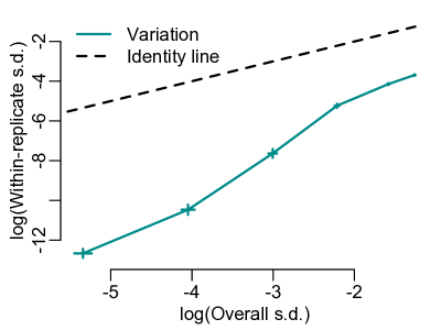
Figure 6: Relative variability in the $\ell$-test p-values due to the randomness in $\hat{\lambda}_{j}$. The error bars represent plus or minus two units of standard errors.

This figure suggests that the variability due to sampling of $\tilde{\bm{y}}$ is negligible compared to the monte-carlo variability in the p-values due to the replication of the procedure—we see from Figure 6 that sampling of $\tilde{\bm{y}}$ never accounts for more than about $9\%$ of the overall standard deviation (or about $0.8\%$ of the overall variation). This suggests that even though randomized due to sampling of $\tilde{\bm{y}}$, the p-values we obtain are stable.

Finally, note that an alternate way of doing cross-validation that does not introduce the randomness in the procedure due to sampling $\tilde{\bm{y}}$ is by cross-validating on $(\hat{\bm{y}}_{j},\bm{X}_{-j})$ instead, where $\hat{\bm{y}}_{j}$ is the projection of $\bm{y}$ on the columnspace of $\bm{X}_{-j}$ (and is the non-zero-mean component of $\tilde{\bm{y}}$, when sampled from $\bm{y}\mid\bm{S}^{(j)}$ under $H_{j}$). Note that computation of $\ell$-distribution based on either of $(\hat{\bm{y}}_{j},\bm{X}_{-j})$ or $(\tilde{\bm{y}},\bm{X}_{-j})$ would exactly be the same. Even though we have established that the sampling of $\tilde{\bm{y}}$ introduces negligible randomness in the $\ell$-test p-value, one might wonder why introduce any randomness at all in the first place and not cross-validate on $(\hat{\bm{y}}_{j},\bm{X}_{-j})$? In Figure 7, we compare three possible datasets we can cross-validate on to choose $\lambda$: $(\tilde{\bm{y}},\bm{X}_{-j})$ (our default choice), $(\hat{\bm{y}}_{j},\bm{X}_{-j})$ and $(\bm{y},\bm{X})$. Note that, as described in Section 2.4, the last choice is not valid as the chosen $\lambda$ will not be a function of the sufficient statistic, however as this is cross-validating on the full dataset, we can expect this chosen $\lambda$ to have the ‘optimal performance’ and the resulting power curve can be used as a benchmark. Indeed, Figure 7 shows that choosing $\lambda$ based on $(\hat{\bm{y}}_{j},\bm{X}_{-j})$ suffers a detriment as compared to our recommended choice (which also performs almost similarly to cross-validating on the full $(\bm{y},\bm{X})$), providing further justification for it.

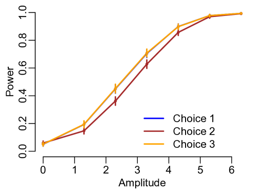
Figure 7: We use exactly the same setting as in the left panel of Figure 2. Choice 1,2 and 3 denote choosing $\lambda$ by cross-validating on $(\tilde{\bm{y}},\bm{X}_{-j})$, $(\hat{\bm{y}}_{j},\bm{X}_{-j})$ and $(\bm{y},\bm{X})$, respectively. The curves for Choice 1 and 3 are on top of each other. The error bars represent plus or minus two standard errors.

Appendix F Further Experiments

F.1 Performance of the $\ell$-test under different settings

To explore further aspects of the performance of the $\ell$-test, we test its performance under an additional setting, with the results are summarized in Figure 8. We see that in this case, similar to Figure 2, the power of the $\ell$-test increases with increasing amplitude, but almost overlapping with that of the one-sided $t$-test. Note that, as follows from Appendix B, in this case where our particular choice of the design matrix is closer to un-identifiability, the $\ell$-test is more sure about its guess of the sign of the alternate $\beta_{j}$ as compared to the $d=50$ case.

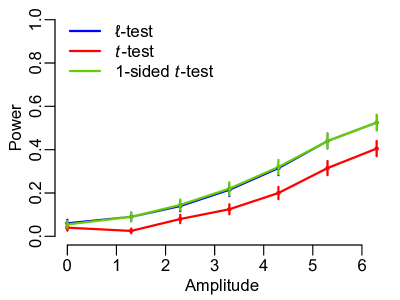
Figure 8: Exactly the same setting as in the left panel of Figure 2 but with $d=90$. The error bars represent plus or minus two standard errors.

F.2 Robustness of the $\ell$-test to violations of the linear model assumptions

In this section, we extend the results in Section 5.2 by performing more extensive experiments to empirically evaluate the robustness of the validity of the $\ell$-test to the violations in the assumptions of the Gaussian linear model. We will be under the same exact setup of Section 5.2 and will consider the following settings, each aimed at testing a specific kind of violation.

• Setting 1 (Violation of the Gaussianity of errors—effect of heavy tails): For each specific value of $(n,d)$, we draw i.i.d. errors from a $t$ distribution with $\nu$ degrees of freedom. We vary $\nu$ between 30 and 2. For $\nu>2$, we also standardize the mean zero errors with the standard deviation of the $t_{\nu}$ distribution. We do not do this for $t_{2}$ as it does not have a finite second moment. As $\nu$ varies from 30 to 2, the tails of $t_{\nu}$ gets fatter as compared to the normal distribution. We summarize our results in Figure 9.

• Setting 2 (Violation of the Gaussianity of errors—effect of skewness): We consider a setup similar to that in Setting 1 but instead consider Gamma distributed error with scale parameter 1 and shape parameter, $\alpha$. We vary $\alpha$ between 1 and 10 and for each error draw, we standardize the error with the mean and standard deviation of the Gamma$(1,\alpha)$ distribution. This error distribution is asymmetric for smaller values of $\alpha$ and moves towards symmetry as the value of $\alpha$ increases. We summarize our results in Figure 10.

• Setting 3 (Violation of homoskedasticity of error): We again consider a similar setup as above, but change the error distribution as follows: For design matrix, $\bm{X}$, we define $m_{\bm{X}}$ to be the median of the mean of the rows, that is median of the elements of $\bm{X}\bm{1}/d$. Let $r_{i}$ denote mean of the $i^{\mathrm{th}}$ row of the design matrix, we generate the error vector $\bm{\epsilon}=(\epsilon_{1},\dots,\epsilon_{n})^{T}$, where,

  $$\epsilon_{i}\stackrel{{\scriptstyle i.i.d.}}{{\sim}}\begin{cases}\mathcal{N}(0,1),&\textrm{ if }r_{i}\leq m_{\bm{X}}\\ \mathcal{N}(0,\eta^{2}),&\textrm{ if }r_{i}>m_{\bm{X}}\end{cases},$$

  where $\eta^{2}>0$ is a quantity, specified by us, that controls the heteroskedasticity in the error term. For $\eta=1$, the distribution is homoskedastic while becomes heteroskedastic for larger and smaller values of $\eta$. We vary $\eta^{2}$ in the set $\{0.01,0.25,0.5,1,4,8\}$ and compare the performance of the two tests for each of these values. The results are summarized in Figure 11.

• Setting 4 (Violation of the linearity assumption): In this setting we test the robustness of the two tests to non-linearity in the model. We consider settings with similar specifications as the above three cases but with i.i.d. homoskedastic, normal errors with variance $\sigma^{2}$. In this case, for design matrix, $\bm{X}$, and error term, $\bm{\epsilon}$, we define,

  $$y_{i}=(\bm{X}_{i}^{\delta})^{T}\bm{\beta}+\epsilon_{i},$$

  where $\delta$ is variable we will control, and $\bm{X}_{i}^{\delta}$ denotes a vector whose $j^{\mathrm{th}}$ entry is the $j^{\mathrm{th}}$ entry of $\bm{X}_{i}$ raised to the exponent, $\delta$. $\delta=1$ recovers the usual linear model and larger departure of $\delta$ from 1 imparts higher degree of non-linearity to the model. We vary $\delta$ in the set, $\{0.3,0.5,1,2,3,4\}$ and summarize the results in Figure 12.

The results from all the three simulations suggest that the $\ell$-test and the $t$-test have similar degree of tolerance against violations of the linear model assumptions. The $t$-test exhibits robustness against the violation of the Gaussianity assumption in the error term, as Figures 9 and 10 indicate and we see a similar behavior for the $\ell$-test. Notably, the performance of $\ell$-test is almost similar to that of the $t$-test in the extreme cases, such as when the degrees of freedom for the error $t$-distribution is 2 in Figure 9 (indicating fat tails of the error distribution) or when the shape parameter of the centered gamma distributed error is 1 (which essentially is a centered exponential distribution with rate 1, indicating a high degree of skeweness in the error term). For Setting 3 with heteroskedastic errors, we see from Figure 11 that the $\ell$-test’s size does depart from its nominal target of $0.05$ as $\eta$ moves away from 1 (which is the homoskedastic case). However, this departure is of a similar degree as that of the $t$-test, so that both the tests exhibit similar robustness properties under this setting. From Figure 12 as well, we see that both the $t$-test and the $\ell$-test are robust to the violation of non-linearity.

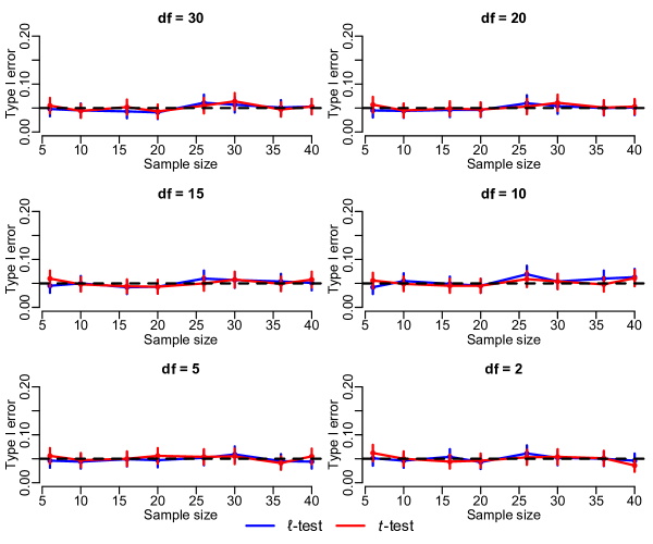
Figure 9: Effect of $t$-distributed errors on the size of the $\ell$-test and the $t$-test, for different degrees of freedom. The error bars represent plus or minus two standard errors.

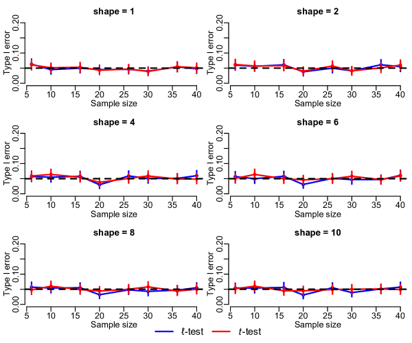
Figure 10: Effect of Gamma distributed errors (with scale parameter 1) on the size of the $\ell$-test and the $t$-test, for different values of the shape parameter. The error bars represent plus or minus two standard errors.

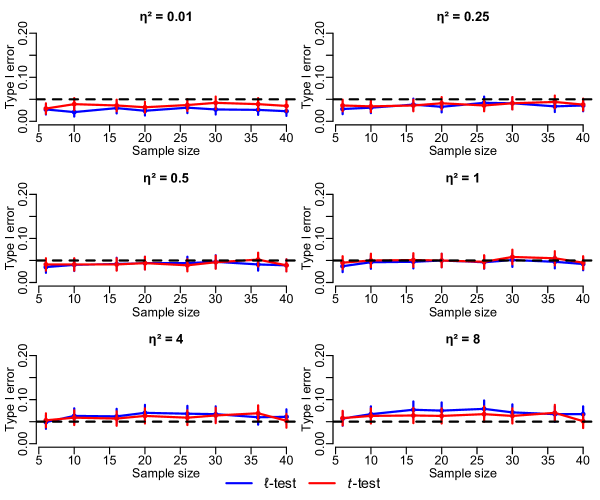
Figure 11: Effect of heteroskedasticity on the size of the $\ell$-test and the $t$-test. Values of $\eta$ away from 1 indicate higher degree of heteroskedasticity. The error bars represent plus or minus two standard errors.

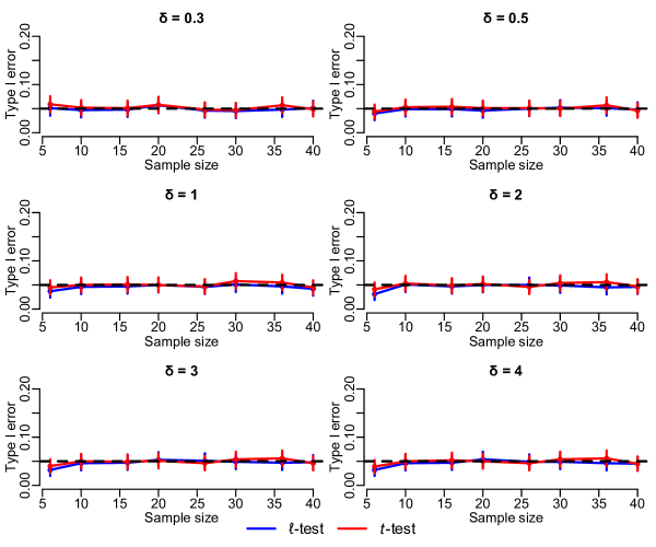
Figure 12: Effect of non-linearity on the size of the $\ell$- and the $t$-test. Departure of the exponent, $\delta$ away from 1 indicates higher degree of non-linearity in the model. The error bars represent plus or minus two standard errors.

F.3 Comparison of the various confidence intervals in the linear model

In this section, we summarize the full results of our simulations comparing the various procedures of obtaining confidence intervals for $\beta_{j}$. We consider four different experimental settings in Figure 13 (studying the effect of varying the amplitude with $d$ much smaller than $n$ ), Figure 14 (studying the effect of varying the amplitude with $d$ and $n$ close), Figure 15 (studying the effect of varying the sparsity in $\bm{\beta}$) and Figure 16 (studying the effect of varying the inter-variable correlations). The linear model we consider has exactly the same specifications as in Section 5.3 and the captions of the respective figures contain the further details. For the $\ell$-test confidence interval, we consider the performance of the procedure when both the min rule and the 1se rule is used to choose $\lambda$. In addition to our observations in Section 5.3 and similar to those in Section F.1, we observe from Figure 14 that the gap between the average length of the confidence interval obtained by inverting the one-sided $t$-test and the $\ell$-test confidence interval is even smaller when $d=90$, and can again be justified by our observations in Appendix B. We also see that, except for the cases when the vector $\bm{\beta}$ is very dense, the performance of the 1se rule and the min rule is almost identical, despite the former being a stricter selection rule. Even though the former chops-off a larger mass from the distribution of $u_{1}$, it is less likely that this region significantly overlaps with the corresponding $5\%$ rejection region and hence the corresponding smoothed out statistic (as described in Section 2.3) under both the rules have almost similar distribution in the 5$\%$ rejection region. However, as is evident from Figure 15, the 1se rule does perform worse than the min rule when the most of the entries of $\bm{\beta}$ are signals and can be attributed to the fact that in this case the LASSO is not a good estimator of $\bm{\beta}$ and most of our intuitions break down.

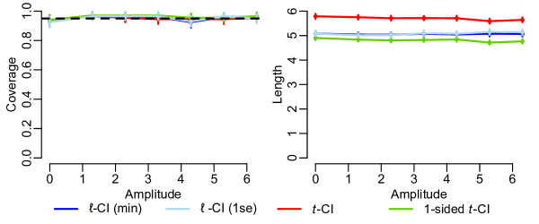
Figure 13: Length and coverage of various $95\%$ confidence intervals. We set $n=100,d=50,k=5,\bm{\Sigma}=\bm{I},\sigma=1$ and vary $A$. The error bars represent plus or minus two standard errors.

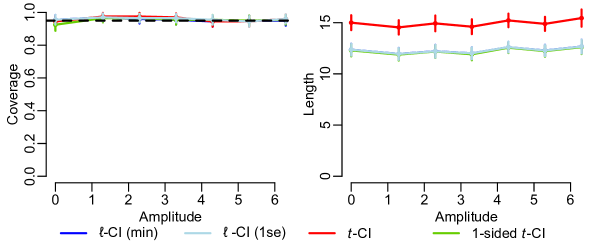
Figure 14: Length and coverage of various $95\%$ confidence intervals. We set $n=100,d=90,k=5,\bm{\Sigma}=\bm{I},\sigma=1$ and vary $A$. The error bars represent plus or minus two standard errors.

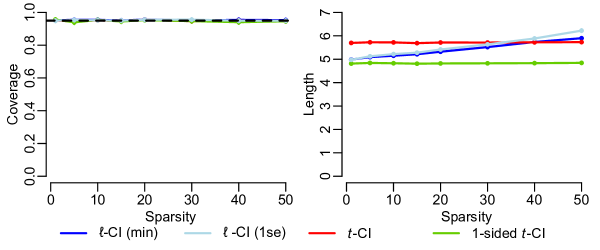
Figure 15: Length and coverage of various $95\%$ confidence intervals while varying the sparsity. We set $n=100,d=90,A=4.3,\bm{\Sigma}=\bm{I},\sigma=1$ and vary $k$. The error bars represent plus or minus two standard errors.

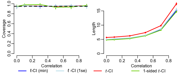
Figure 16: Length and coverage of various $95\%$ confidence intervals while varying the inter-variable correlation. We set $n=100,d=90,A=4.3,k=4,\bm{\Sigma}_{ij}=\rho^{|i-j|},\sigma=1$ and vary $\rho$. The error bars represent plus or minus two standard errors.

F.4 LASSO selection-adjusted confidence sets for linear model coefficients

Expanding on Section 5.4, we compare the various conditional-on-LASSO-selection inference methods under another setting where $d=90$, with the results plotted in Figure 17. As in Figure 5, there is practically no difference between the performance of $\underline{\hat{C}}_{j}^{\lambda}$ and $\underline{\hat{C}}_{j}^{*\lambda}$ but, unlike in Figure 5, Liu et al. (2018) performs quite similarly to them as well. The reason for this is that, as noted in Section 1.3, Liu et al. (2018)’s method assumes known $\sigma^{2}$ (and hence we provide it the true value of $\sigma^{2}$ in both this simulation and that of Figure 5) while the $\ell$-test does not. Unknown $\sigma^{2}$ is what necessitates the second component of the sufficient statistic $\bm{S}^{(j)}$, namely, $\bm{y}^{T}\bm{y}$, which the $\ell$-test conditions on but Liu et al. (2018)’s method does not. This difference becomes information-theoretically more pronounced as $d$ approaches $n$, as it does in the simulation in Figure 17, because the residual degrees of freedom decreases, resulting in a relative power loss for the $\ell$-test-based confidence intervals that approximately offsets the benefit of the $\ell$-test. To confirm this explanation, we can easily derive a version of the $\ell$-test and corresponding conditional confidence intervals that assumes $\sigma^{2}$ is known and hence does not condition on $\bm{y}^{T}\bm{y}$ (see footnote in Section 6). This is plotted as dashed curves in Figure 17, and as expected these methods again provide consistently shorter confidence intervals than the method in Liu et al. (2018).

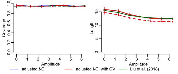
Figure 17: We consider the exact same setting as Figure 5 but with $d=90$. The dashed curves represent the counterparts of the corresponding $\ell$-test procedures with known $\sigma^{2}$. The error bars represent plus or minus two standard errors.

Appendix G Inverting the one-sided $t$-test

In this section, we describe the confidence interval obtained by inverting the one-sided $t$-test, as mentioned in Section 5.3. For the linear model, $\bm{y}\sim N_{n}(\bm{X}\bm{\beta},\sigma^{2}\bm{I}_{n})$, the one-sided $t$-test tests $H_{j}(\gamma):\beta_{j}=\gamma$ by rejecting for large values of the $t$-test statistic if $\beta_{j}>\gamma$ and and for small values, if $\beta_{j}<\gamma$. In case $\beta_{j}=\gamma$, we, without any loss of generality, fix the convention of rejecting for small values of the $t$-test statistic, however, the validity of the test is not affected if rejecting for large values as well. Thus, with this convention, the one-sided $t$-test rejects $H_{j}(\gamma)$ when $\frac{\hat{\beta}_{j,\mathrm{OLS}}-\gamma}{\hat{\mathrm{SE}}\left(\hat{\beta}_{j,\mathrm{OLS}}\right)}>t_{\alpha;n-d}$, if $\beta_{j}>\gamma$ and when $\frac{\hat{\beta}_{j,\mathrm{OLS}}-\gamma}{\hat{\mathrm{SE}}\left(\hat{\beta}_{j,\mathrm{OLS}}\right)}<-t_{\alpha;n-d}$, if $\beta_{j}\leq\gamma$. Here $t_{\alpha;n-d}$ is the quantile of the $t_{n-d}$ distribution putting mass $\alpha$ on its upper tail. Inverting this test gives the following one-sided $100(1-\alpha)\%$ confidence interval,

$$C^{t}_{\mathrm{1-sided}}=\begin{cases}\left[\hat{\beta}_{j,\mathrm{OLS}}\pm t_{\alpha;n-d}\hat{\mathrm{SE}}\left(\hat{\beta}_{j,\mathrm{OLS}}\right)\right],&\textrm{ if }\beta_{j}\in\left[\hat{\beta}_{j,\mathrm{OLS}}\pm t_{\alpha;n-d}\hat{\mathrm{SE}}\left(\hat{\beta}_{j,\mathrm{OLS}}\right)\right]\\ \left[\beta_{j},\hat{\beta}_{j,\mathrm{OLS}}+t_{\alpha;n-d}\hat{\mathrm{SE}}\left(\hat{\beta}_{j,\mathrm{OLS}}\right)\right),&\textrm{ if }\beta_{j}<\hat{\beta}_{j,\mathrm{OLS}}-t_{\alpha;n-d}\hat{\mathrm{SE}}\left(\hat{\beta}_{j,\mathrm{OLS}}\right)\\ \left(\hat{\beta}_{j,\mathrm{OLS}}-t_{\alpha;n-d}\hat{\mathrm{SE}}\left(\hat{\beta}_{j,\mathrm{OLS}}\right),\beta_{j}\right),&\textrm{ if }\beta_{j}>\hat{\beta}_{j,\mathrm{OLS}}+t_{\alpha;n-d}\hat{\mathrm{SE}}\left(\hat{\beta}_{j,\mathrm{OLS}}\right).\end{cases}$$

Note that the above interval is indeed an oracle interval as one needs to know the exact value of $\beta_{j}$ to construct it. Furthermore note that when $\beta_{j}>\hat{\beta}_{j,\mathrm{OLS}}+t_{\alpha;n-d}\hat{\mathrm{SE}}\left(\hat{\beta}_{j,\mathrm{OLS}}\right)$, the interval surely misses the target parameter, $\beta_{j}$, and this is because of the one-sided nature of the test when we are testing at the true parameter, $\gamma=\beta_{j}$. In case we were rejecting for large values of the $t$-test statistic on observing $\beta_{j}$, we would get an open interval in the case when $\beta_{j}<\hat{\beta}_{j,\mathrm{OLS}}-t_{\alpha;n-d}\hat{\mathrm{SE}}\left(\hat{\beta}_{j,\mathrm{OLS}}\right)$ instead.

References

- Adichie (1967) J. N. Adichie. Asymptotic Efficiency of a Class of Non-Parametric Tests for Regression Parameters. The Annals of Mathematical Statistics, 38(3):884 – 893, 1967. doi: 10.1214/aoms/1177698882. URL https://doi.org/10.1214/aoms/1177698882.
- Bachoc et al. (2016) F. Bachoc, D. Preinerstorfer, and L. Steinberger. Uniformly valid confidence intervals post-model-selection. The Annals of Statistics, 48, 11 2016. doi: 10.1214/19-AOS1815.
- Barber and Candès (2015) R. F. Barber and E. J. Candès. Controlling the false discovery rate via knockoffs. The Annals of Statistics, 43(5):2055 – 2085, 2015. doi: 10.1214/15-AOS1337. URL https://doi.org/10.1214/15-AOS1337.
- Barber and Janson (2022) R. F. Barber and L. Janson. Testing goodness-of-fit and conditional independence with approximate co-sufficient sampling. The Annals of Statistics, 50(5):2514 – 2544, 2022. doi: 10.1214/22-AOS2187. URL https://doi.org/10.1214/22-AOS2187.
- Bartlett (1937) M. S. Bartlett. Properties of sufficiency and statistical tests. Proceedings of the Royal Society of London. Series A-Mathematical and Physical Sciences, 160(901):268–282, 1937.
- Berge (1963) C. Berge. Topological spaces including a treatment of multi-valued functions, vector spaces and convexity. Edinburgh-London: Oliver & Boyd, Ltd. XIII, 270 p. (1963)., 1963.
- Berk et al. (2013) R. Berk, L. Brown, A. Buja, K. Zhang, and L. Zhao. Valid post-selection inference. The Annals of Statistics, 41(2):802 – 837, 2013. doi: 10.1214/12-AOS1077. URL https://doi.org/10.1214/12-AOS1077.
- Candès et al. (2018) E. Candès, Y. Fan, L. Janson, and J. Lv. Panning for gold: Model-X knockoffs for high-dimensional controlled variable selection. Journal of the Royal Statistical Society: Series B, 80(3):551–577, 2018.
- Cox (1975) D. R. Cox. A note on data-splitting for the evaluation of significance levels. Biometrika, 62:441–444, 1975. URL https://api.semanticscholar.org/CorpusID:119955345.
- Dai et al. (2022) C. Dai, B. Lin, X. Xing, and J. S. Liu. False discovery rate control via data splitting. Journal of the American Statistical Association, 0(0):1–18, 2022. doi: 10.1080/01621459.2022.2060113. URL https://doi.org/10.1080/01621459.2022.2060113.
- Efron (1979) B. Efron. Bootstrap Methods: Another Look at the Jackknife. The Annals of Statistics, 7(1):1 – 26, 1979. doi: 10.1214/aos/1176344552. URL https://doi.org/10.1214/aos/1176344552.
- Efron et al. (2004) B. Efron, T. Hastie, I. Johnstone, and R. Tibshirani. Least angle regression. The Annals of Statistics, 32(2):407 – 499, 2004. doi: 10.1214/009053604000000067. URL https://doi.org/10.1214/009053604000000067.
- Fisher (1922) R. A. Fisher. The goodness of fit of regression formulae, and the distribution of regression coefficients. Journal of the Royal Statistical Society, 85(4):597–612, 1922.
- Fithian et al. (2014) W. Fithian, D. Sun, and J. Taylor. Optimal inference after model selection. 10 2014.
- Freedman (1981) D. A. Freedman. Bootstrapping Regression Models. The Annals of Statistics, 9(6):1218 – 1228, 1981. doi: 10.1214/aos/1176345638. URL https://doi.org/10.1214/aos/1176345638.
- Friedman et al. (2010) J. Friedman, R. Tibshirani, and T. Hastie. Regularization paths for generalized linear models via coordinate descent. Journal of Statistical Software, 33(1):1–22, 2010. doi: 10.18637/jss.v033.i01.
- Friedman (1937) M. Friedman. The use of ranks to avoid the assumption of normality implicit in the analysis of variance. Journal of the American Statistical Association, 32(200):675–701, 1937. doi: 10.1080/01621459.1937.10503522. URL https://www.tandfonline.com/doi/abs/10.1080/01621459.1937.10503522.
- Gutenbrunner et al. (1993) C. Gutenbrunner, J. JurečKová, R. Koenker, and S. Portnoy. Tests of linear hypotheses based on regression rank scores. Journal of Nonparametric Statistics, 2(4):307–331, Jan. 1993. ISSN 1048-5252. doi: 10.1080/10485259308832561.
- Habiger and Peña (2014) J. D. Habiger and E. A. Peña. Compound p-value statistics for multiple testing procedures. Journal of Multivariate Analysis, 126:153–166, 2014. ISSN 0047-259X. doi: https://doi.org/10.1016/j.jmva.2014.01.007. URL https://www.sciencedirect.com/science/article/pii/S0047259X14000153.
- Hajek (1962) J. Hajek. Asymptotically Most Powerful Rank-Order Tests. The Annals of Mathematical Statistics, 33(3):1124 – 1147, 1962. doi: 10.1214/aoms/1177704476. URL https://doi.org/10.1214/aoms/1177704476.
- Hoff (2022) P. Hoff. Smaller p-values via indirect information. Journal of the American Statistical Association, 117(539):1254–1269, 2022. doi: 10.1080/01621459.2020.1844720. URL https://doi.org/10.1080/01621459.2020.1844720.
- Hoff and Yu (2019) P. Hoff and C. Yu. Exact adaptive confidence intervals for linear regression coefficients. Electronic Journal of Statistics, 13(1):94 – 119, 2019. doi: 10.1214/18-EJS1517. URL https://doi.org/10.1214/18-EJS1517.
- Huang and Janson (2020) D. Huang and L. Janson. Relaxing the assumptions of knockoffs by conditioning. Ann. Statist., 48(5):3021–3042, 10 2020. doi: 10.1214/19-AOS1920. URL https://doi.org/10.1214/19-AOS1920.
- Jaeckel (1972) L. A. Jaeckel. Estimating Regression Coefficients by Minimizing the Dispersion of the Residuals. The Annals of Mathematical Statistics, 43(5):1449 – 1458, 1972. doi: 10.1214/aoms/1177692377. URL https://doi.org/10.1214/aoms/1177692377.
- Javanmard and Montanari (2014) A. Javanmard and A. Montanari. Confidence intervals and hypothesis testing for high-dimensional regression. Journal of Machine Learning Research, 15(82):2869–2909, 2014. URL http://jmlr.org/papers/v15/javanmard14a.html.
- Kruskal and Wallis (1952) W. H. Kruskal and W. A. Wallis. Use of ranks in one-criterion variance analysis. Journal of the American Statistical Association, 47(260):583–621, 1952. ISSN 01621459. URL http://www.jstor.org/stable/2280779.
- Lee and Ren (2024) J. Lee and Z. Ren. Boosting e-bh via conditional calibration, 2024.
- Lee et al. (2016) J. D. Lee, D. L. Sun, Y. Sun, and J. E. Taylor. Exact post-selection inference, with application to the lasso. The Annals of Statistics, 44(3):907 – 927, 2016. doi: 10.1214/15-AOS1371. URL https://doi.org/10.1214/15-AOS1371.
- Lehmann and Scheffé (1955) E. L. Lehmann and H. Scheffé. Completeness, similar regions, and unbiased estimation: Part ii. Sankhyā: The Indian Journal of Statistics (1933-1960), 15(3):219–236, 1955. ISSN 00364452. URL http://www.jstor.org/stable/25048243.
- Lei and Bickel (2020) L. Lei and P. J. Bickel. An assumption-free exact test for fixed-design linear models with exchangeable errors. Biometrika, 108(2):397–412, 09 2020. ISSN 0006-3444. doi: 10.1093/biomet/asaa079. URL https://doi.org/10.1093/biomet/asaa079.
- Li and Fithian (2021) X. Li and W. Fithian. Whiteout: when do fixed-x knockoffs fail?, 2021.
- Liu et al. (2018) K. Liu, J. Markovic, and R. Tibshirani. More powerful post-selection inference, with application to the lasso, 2018.
- Liu et al. (2021+) M. Liu, E. Katsevich, L. Janson, and A. Ramdas. Fast and powerful conditional randomization testing via distillation. Biometrika, 2021+. To Appear.
- Luo et al. (2022) Y. Luo, W. Fithian, and L. Lei. Improving knockoffs with conditional calibration, 2022.
- Panigrahi et al. (2021) S. Panigrahi, J. Taylor, and A. Weinstein. Integrative methods for post-selection inference under convex constraints. The Annals of Statistics, 49(5):2803–2824, 2021.
- Pitman (1937) E. J. G. Pitman. Significance tests which may be applied to samples from any populations. ii. the correlation coefficient test. Supplement to the Journal of the Royal Statistical Society, 4(2):225–232, 1937. ISSN 14666162. URL http://www.jstor.org/stable/2983647.
- Pitman (1938) E. J. G. Pitman. Significance Tests which May be Applied to Samples from any Populations: III. The Analysis of Variance Test. Biometrika, 29(3-4):322–335, 02 1938. ISSN 0006-3444. doi: 10.1093/biomet/29.3-4.322. URL https://doi.org/10.1093/biomet/29.3-4.322.
- R Core Team (2024) R Core Team. R: A Language and Environment for Statistical Computing. R Foundation for Statistical Computing, Vienna, Austria, 2024. URL https://www.R-project.org/.
- Ren and Barber (2023) Z. Ren and R. F. Barber. Derandomised knockoffs: leveraging e-values for false discovery rate control. Journal of the Royal Statistical Society Series B: Statistical Methodology, page qkad085, 09 2023. ISSN 1369-7412. doi: 10.1093/jrsssb/qkad085. URL https://doi.org/10.1093/jrsssb/qkad085.
- Rhee et al. (2006) S.-Y. Rhee, J. Taylor, G. Wadhera, A. Ben-Hur, D. L. Brutlag, and R. W. Shafer. Genotypic predictors of human immunodeficiency virus type 1 drug resistance. Proceedings of the National Academy of Sciences, 103(46):17355–17360, 2006. doi: 10.1073/pnas.0607274103. URL https://www.pnas.org/doi/abs/10.1073/pnas.0607274103.
- Rinaldo et al. (2016) A. Rinaldo, L. Wasserman, M. G’Sell, J. Lei, and R. Tibshirani. Bootstrapping and sample splitting for high-dimensional, assumption-free inference. The Annals of Statistics, 47, 11 2016. doi: 10.1214/18-AOS1784.
- Rosset and Zhu (2007) S. Rosset and J. Zhu. Piecewise linear regularized solution paths. The Annals of Statistics, 35(3):1012 – 1030, 2007. doi: 10.1214/009053606000001370. URL https://doi.org/10.1214/009053606000001370.
- Spector and Janson (2022) A. Spector and L. Janson. Powerful knockoffs via minimizing reconstructability. Annals of Statistics, 50(1):252–276, 2022.
- Stephens (2012) M. Stephens. Goodness-of-fit and sufficiency: Exact and approximate tests. Methodology and Computing in Applied Probability, 14, 09 2012. doi: 10.1007/s11009-011-9267-2.
- Sur and Candès (2019) P. Sur and E. J. Candès. A modern maximum-likelihood theory for high-dimensional logistic regression. Proceedings of the National Academy of Sciences, 116(29):14516–14525, 2019.
- Tian and Taylor (2018) X. Tian and J. Taylor. Selective inference with a randomized response. The Annals of Statistics, 46(2):679–710, 2018.
- Tibshirani et al. (2005) R. Tibshirani, M. Saunders, S. Rosset, J. Zhu, and K. Knight. Sparsity and smoothness via the fused lasso. Journal of the Royal Statistical Society Series B: Statistical Methodology, 67(1):91–108, 2005.
- Tibshirani et al. (2016) R. Tibshirani, J. Taylor, R. Lockhart, and R. Tibshirani. Exact post-selection inference for sequential regression procedures. Journal of the American Statistical Association, 111:600–620, 04 2016. doi: 10.1080/01621459.2015.1108848.
- Tseng (2001) P. Tseng. Convergence of a block coordinate descent method for nondifferentiable minimization. J. Optim. Theory Appl., 109(3):475–494, jun 2001. ISSN 0022-3239. doi: 10.1023/A:1017501703105. URL https://doi.org/10.1023/A:1017501703105.
- Tukey (1958) J. Tukey. Bias and confidence in not quite large samples. Annals of Mathematical Statistics, 29:614, 01 1958. doi: 10.1214/aoms/1177706647.
- van de Geer et al. (2014) S. van de Geer, P. Bühlmann, Y. Ritov, and R. Dezeure. On asymptotically optimal confidence regions and tests for high-dimensional models. The Annals of Statistics, 42(3):1166 – 1202, 2014. doi: 10.1214/14-AOS1221. URL https://doi.org/10.1214/14-AOS1221.
- Xing et al. (2023) X. Xing, Z. Zhao, and J. S. Liu. Controlling false discovery rate using gaussian mirrors. Journal of the American Statistical Association, 118(541):222–241, 2023. doi: 10.1080/01621459.2021.1923510. URL https://doi.org/10.1080/01621459.2021.1923510.
- Zhang and Zhang (2014) C.-H. Zhang and S. S. Zhang. Confidence intervals for low dimensional parameters in high dimensional linear models. Journal of the Royal Statistical Society. Series B (Statistical Methodology), 76(1):217–242, 2014. ISSN 13697412, 14679868. URL http://www.jstor.org/stable/24772752.
- Zhao et al. (2022) Q. Zhao, P. Sur, and E. J. Candes. The asymptotic distribution of the mle in high-dimensional logistic models: Arbitrary covariance. Bernoulli, 28(3):1835–1861, 2022.