SAM: Semi-Active Mechanism for Extensible Continuum Manipulator and Real-time Hysteresis Compensation Control Algorithm

Abstract

Cable-Driven Continuum Manipulators (CDCMs) enable scar-free procedures via natural orifices and improve target lesion accessibility through curved paths. However, CDCMs face limitations in workspace and control accuracy due to non-linear cable effects causing hysteresis. This paper introduces an extensible CDCM with a Semi-active Mechanism (SAM) to expand the workspace via translational motion without additional mechanical elements or actuation. We collect a hysteresis dataset using 8 fiducial markers and RGBD sensing. Based on this dataset, we develop a real-time hysteresis compensation control algorithm using the trained Temporal Convolutional Network (TCN) with a 1ms time latency, effectively estimating the manipulator’s hysteresis behavior. Performance validation through random trajectory tracking tests and box pointing tasks shows the proposed controller significantly reduces hysteresis by up to 69.5% in joint space and approximately 26% in the box pointing task.

Keywords: computer-assisted surgery, continuum robots, flexible manipulator, extensible continuum, cable actuation, hysteresis compensation

I Introduction

Rigid surgical manipulator encounter difficulties in accessing lesions, especially in surgeries involving internal organs like the small and large intestines[1]. In contrast, Cable-Driven Continuum Manipulators (CDCMs), with their flexible and bendable property, are expected to enable minimally invasive surgery by navigating through complex internal organs [2, 3, 4, 5]. CDCMs are emerging as a next-generation surgical manipulation technology.

Miniaturization of CDCMs for endoscopic surgery arise challenge due to size constraints [6]. While miniaturization is crucial for safe insertion without damaging tissue, it inherently restricts the workspace [7, 8], making it difficult for surgeons to navigate and access diverse target lesions. This conflict between miniaturization and workspace necessitates the development of novel CDCM [9]. Additionally, endoscopic CDCMs leverage cable actuation for insertion into the body, with motors positioned outside the patient. However, various factors such as cable elongation[10], friction[11], twist[12], and coupling[13] induce enlarging hysteresis. This hysteresis behavior hinders precise control of movement, impacting surgical accuracy and potentially extending operating time [14]. These limitations pose a risk to the broader adoption of CDCMs in real-world surgical settings [15].

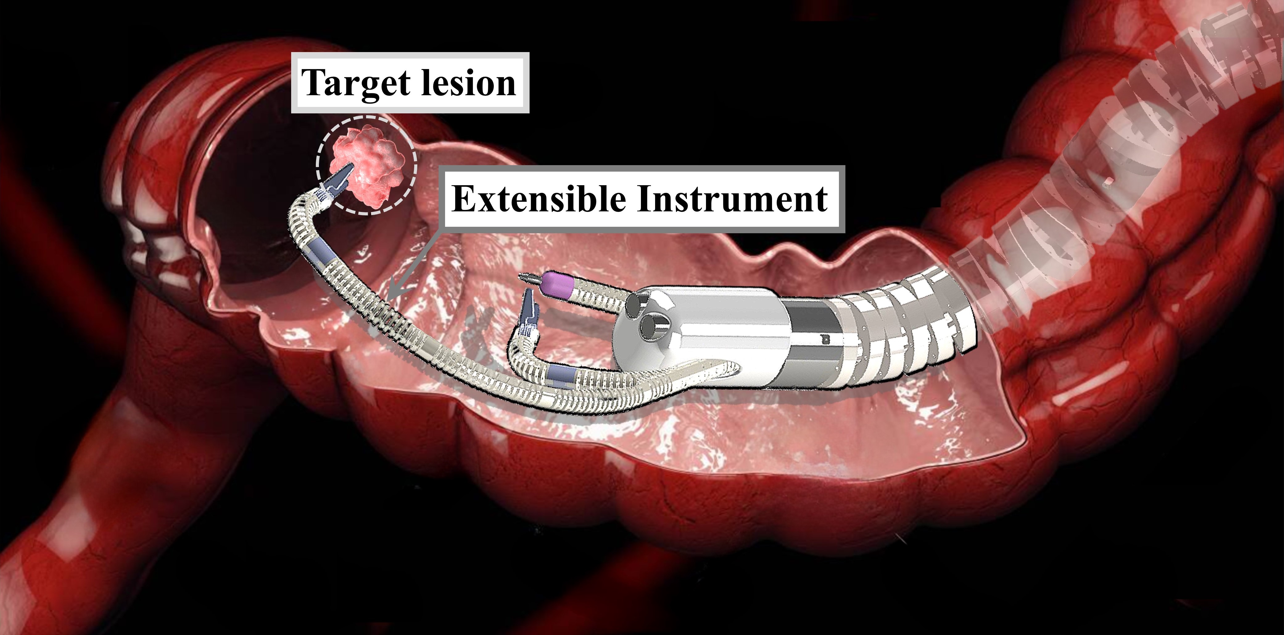
Figure 1: Concept design of the proposed mechanism: By utilizing the semi-active segment, the SAM manipulator can access to the target lesions.

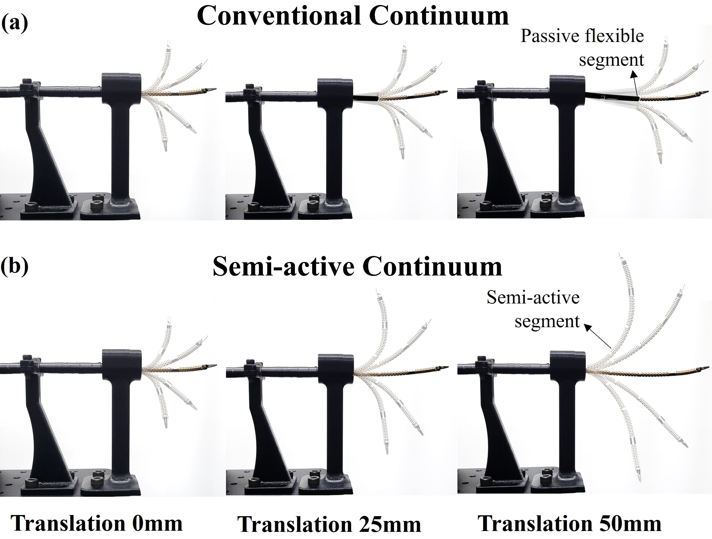
Figure 2: Comparison of workspace during translation between conventional continuum and semi-active continuum: (a) Conventional CDCM with fixed-length segments and a passive flexible segment. This design limits the workspace regardless of manipulator translation and restricts accessibility to the target region. (b) The proposed manipulator with a semi-active segment that lengthens during translation, resulting in an increased workspace within its operational space.

This study introduces the Semi-active Mechanism (SAM) for compact extensible endoscopic CDCMs. Compared to conventional continuum manipulators, the proposed mechanism features ensures that the workspace proportionally expands as the instrument undergoes axial translation (refer to Fig. 1). In a conventional CDCMs, the proximal segment is directly connected to a passive flexible segment (e.g., insertion tube), resulting in a fixed workspace regardless of translation. By introducing SAM, we gain the advantage of extending the workspace without additional active segments (refer to Fig. 2).

The proposed extension mechanism enhances the workspace, but introduces the challenge of hysteresis model variation as the semi-active segment length increases. To address this, we propose a real-time hysteresis compensation control algorithm for the extensible continuum manipulator. The approach involves constructing a hysteresis dataset using an RGBD camera and fiducial markers to capture the relationship between command joint angles and the physical joint angles. We then employ a Temporal Convolutional Network (TCN) to model the complex hysteresis behavior. This trained TCN model estimates the command joint angles for the inputted physical joint angles. Based on this estimation, we develop a real-time control algorithm that actively compensates for hysteresis, leading to enhanced control accuracy. Finally, the performance of the TCN-based compensation method is validated through random joint trajectory tracking and box pointing tasks, demonstrating significant hysteresis reduction in both operational space and joint space.

The main contributions of this paper are summarized as follows: (1) Design and kinematics analysis of the proposed extensible surgical instrument, SAM. (2) Proposal of real-time hysteresis compensation control algorithm in 1ms latency on the proposed instrument. (3) Validation of the proposed control algorithm with random trajectory tracking test and box pointing task suggesting significant hysteresis reduction on both operational space and joint space.

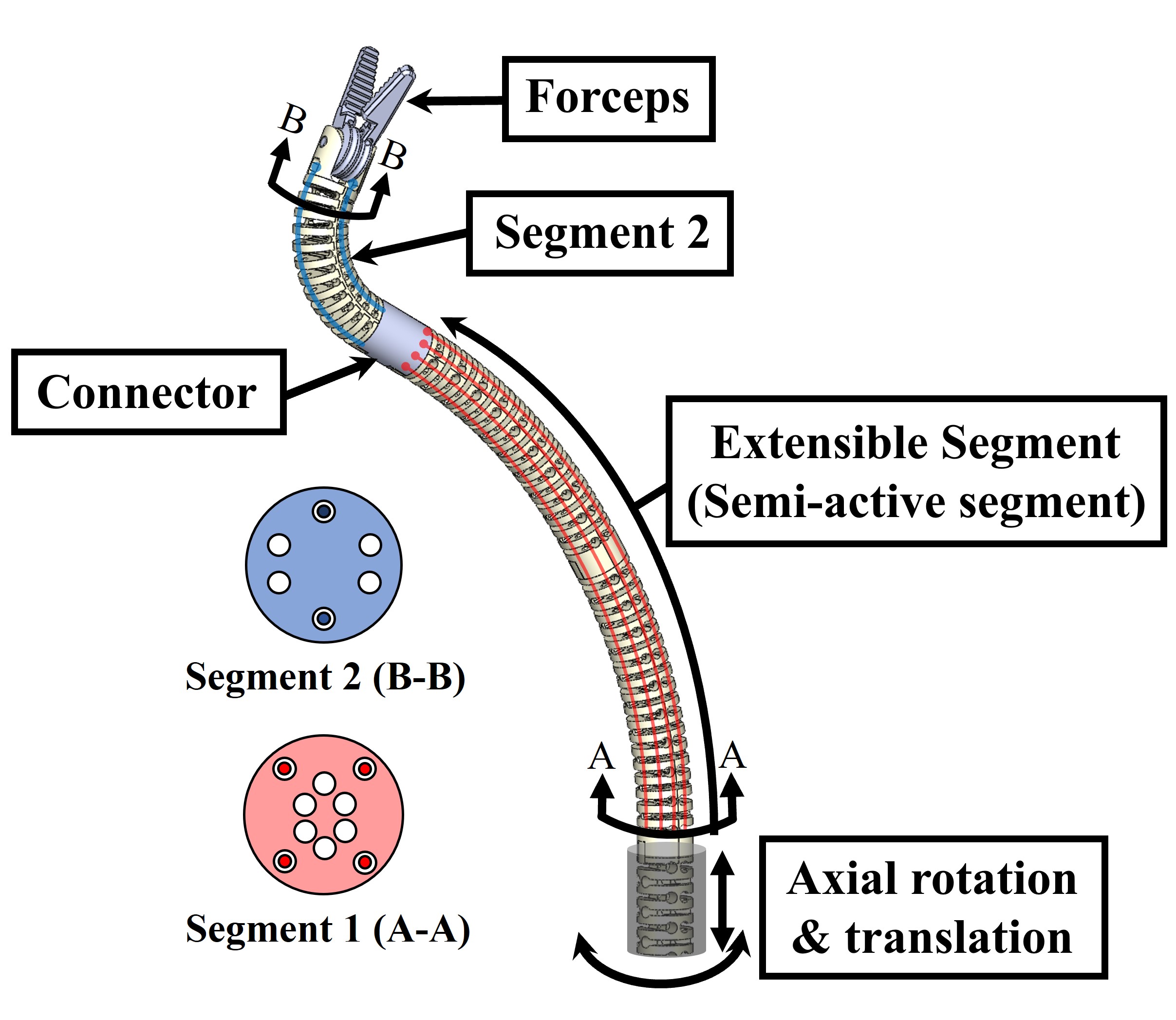
Figure 3: Design of the proposed continuum manipulator : It shows the components of the manipulator and the arrangement of cables in the cross-sections of each segment.

II Related Works

Extensible continuum manipulators have been the subject of various research efforts. These include the use of permanent magnets attached to backbone disks [16], incorporating springs into segments of continuum manipulators to enable extension [17], adjusting length by combining a rack and pinion structure on continuum manipulators [18], automatically attaching and detaching spacer disks on backbone-type continuum manipulators to enable extension [19], and extending the three backbones of continuum manipulators through telescopic principles [20]. Most studies achieve extension and contraction through cable actuation, often incorporating additional mechanical elements such as magnets, springs, and gears. However, these additions can introduce new challenges. For instance, magnetic components often cause control instability due to electromagnetic interference in clinical settings, while gears or springs impede miniaturization efforts. In contrast, the proposed semi-active segment (refer to Fig. 3) enables workspace extensibility without additional mechanical components.

Cable-driven surgical-assistant robots [21] and CDCMs struggles with hysteresis caused by factors like elongation [10], friction [11], twist [12], and coupling [13]. These factors hinder precise control and extend surgical completion times [14]. Previous research has addressed this through analytical modeling [22, 23, 24, 25, 26], learning-based methods [27, 28, 29, 30], and hybrid approaches combining both techniques [31]. Park et al. [30] utilized RGBD cameras and fiducial markers to estimate CDCM poses, employing a Temporal Convolutional Network (TCN)-based hysteresis compensation control algorithm that achieved a 60% reduction in hysteresis. However, their algorithm depends on various parameters and repeatedly utilizes trained models multiple time, resulting in a time latency of approximately 0.05 seconds, which is not be suitable for real-time applications.

Current hysteresis compensation research primarily focuses on general CDCM designs, which are not directly applicable to the proposed manipulator due to the significant impact of extension length on hysteresis behavior. To address this problem, we propose a novel real-time hysteresis compensation model specifically designed for the SAM. This model leverages a dataset of hysteresis behavior under various extension lengths. By utilizing a single trained model that estimates command joint angles from physical joint angles, we achieve real-time compensation control without requiring additional control parameters.

III Kinematics Analysis of Extensible Continuum Manipulator

The proposed continuum manipulator comprises three main components: extensible segment 1, segment 2, and forceps, as illustrated in Fig. 3. Unlike conventional continuum manipulators where the proximal bending segment directly connects to a passive flexible component (e.g., a medical insertion tube), our design incorporates a semi-active segment. This segment allows for extension while maintaining a consistent curvature during bending (see Fig. 2 and Fig. 3). The manipulator has 7 Degrees-of-freedom (DOFs), including axial translation and rotation, pitch and yaw bending of segment 1, pitch bending of segment 2, yaw rotation and grasping of the forceps. It consists of a total of 10 actuation cables, with 4 cables for segment 1, 2 cables for segment 2, and 4 cables for the forceps.

III-A Terminology, Coordinate Frame and Modeling Assumptions

For kinematics modeling, we employ the piecewise constant-curvature approximation, treating each segment of the continuum manipulator as an arc with uniform curvature. The terminology and coordinate frames used in our model are detailed in Table I and illustrated in Fig. 4(a).

• Base coordinate frame of the segment: $O_{i-1}\equiv\left\{{\hat{x}_{i-1}},{\hat{y}_{i-1}},{\hat{z}_{i-1}}\right\}$. The origin of $O_{i-1}$ is at the center of the base of the segment, and axis $z_{i-1}$ is perpendicular to the base plane.

• Base Coordinate frame in bending plane: ${O}^{\prime}_{i-1}\equiv\left\{{{\hat{x}}^{\prime}_{i-1}},{{\hat{y}}^{\prime}_{i-1}},{{\hat{z}}^{\prime}_{i-1}}\right\}$. The origin of ${O}^{\prime}_{i-1}$ aligns with that of $O_{i-1}$, and ${O}^{\prime}_{i-1}$ is derived from $O_{i-1}$ that rotates by $\varphi$ about the z-axis of $O_{i-1}$.

• End coordinate frame in bending plane: ${O}^{\prime}_{i}\equiv\left\{{{\hat{x}}^{\prime}_{i}},{{\hat{y}}^{\prime}_{i}},{{\hat{z}}^{\prime}_{i}}\right\}$. The origin of ${O}^{\prime}_{i}$ is located at the segment’s end center, with its ZY plane parallel to the bending plane of the segment.

• End coordinate frame of the segment : $O_{i}\equiv\left\{{\hat{x}_{i}},{\hat{y}_{i}},{\hat{z}_{i}}\right\}$. The origin of $O_{i}$ aligns with that of ${O}^{\prime}_{i}$, and $O_{i}$ is derived from ${O}^{\prime}_{i}$ that rotates by $-\varphi$ about the z-axis of $O_{i}$.

The overall local coordinate frame definitions for the proposed continuum manipulator are depicted in Fig. 4 (b) and detailed in Table I.

III-B Forward Kinematics of Extensible Segment

We denote the parameters of the extensible segment as $\chi_{\mu}$. As illustrated in Fig. 4 (a), these parameters are represented by $\chi_{\mu}=\left[\kappa,\varphi,\vartheta\right]$. The kinematics of the extensible segment varies based on the protrusion of the semi-active segment, resulting in changes to the arc length corresponding to the translation length $q_{1}$. The arc length of the extensible segment is given by:

$$s=q_{1}+l_{1}$$ (1)

TABLE I: Nomenclature for Extensible Continuum Manipulator

Symbol	Definition
Frame Index ($i$)	Sequential numbering of frames from the base to the EE of the manipulator.
Bending Angle ($\varphi$)	Angle between the bending plane and a reference axis.
Curvature ($k_{x}$)	Curvature around the x-axis.
Curvature ($k_{y}$)	Curvature around the y-axis.
Curvature ($k$)	Overall curvature along the bent segment from its base to the end.
Arc Length ($s_{1}$)	Arc length of the bent extensible segment from its base to the end.
Arc Length ($s_{2}$)	Arc length of segment 2 from its base to the end.
Central Length ($l_{1}$)	The central length of the segment 1.
Translation Length ($q_{1}$)	Translation distance (mm) along the z-axis from the base.
Rotation Angle ($q_{2}$)	Angle of rotation in the roll direction at the base.
Bending Angle of Segment 1 ($q_{3},q_{4}$)	Angles of bending in the pitch and yaw directions of segment 1.
Bending Angle of Segment 2 ($q_{5}$)	The angle by bending in the pitch direction of segment 2.
Rotation Angle of Forceps ($q_{6}$)	The angle by rotating in the yaw direction from forceps.
Bending angle ($\vartheta$)	The total bending angle of each segment.
Homogeneous Transformation Matrix (${}^{i-1}\textrm{T}_{i})$	The homogeneous transformation matrix from $i-1$ to $i$ of extensible segment.
Rotation Matrix ($R_{z}\left(\varphi\right)$)	Rotation matrix that rotates by $\varphi$ about the z-axis.
Rotation Matrix ($R_{x}\left(\kappa s\right)$)	Rotation matrix that rotates by $\kappa s$ about the x-axis.
Rotation Matrix ($R_{z}\left(-\varphi\right)$)	Rotation matrix that rotates by $\varphi$ about the z-axis.
Translation Vector (${}^{i-1}\textrm{P}_{i}$)	Translation vector from $i-1$ to $i$.
Frame ($O_{1_{b}}$)	Manipulator base frame.
Frame ($O^{{}^{\prime}}_{1_{b}}$)	Segment 1 base frame, rotated in the roll direction.
Frame ($O_{1_{e}}$)	End of segment 1 frame.
Frame ($O_{2_{b}}$)	Base of segment 2 frame
Frame ($O_{2_{e}}$)	End of segment 2 frame.
Frame ($O_{ee}$)	End effector frame of the manipulator.

The curvature $\kappa$ of the segment can be represented using the components of curvature along the x-axis $\kappa_{x}$ and y-axis $\kappa_{y}$ of the local frame. The components of curvature, curvature, and the angle $\varphi$ to the bending plane can be expressed as follows:

$$\kappa_{x}=\frac{q_{3}}{s},\;\;\kappa_{y}=\frac{q_{4}}{s}$$

$$\kappa=\sqrt{\kappa_{x}^{2}+\kappa_{y}^{2}}$$

$$\varphi=atan2(\kappa_{x},\kappa_{y})$$ (2)

The angle $\vartheta$ at which the segment is bent, and the translation vector $P(s)$ can be obtained as follows:

$$\vartheta=\sqrt{{q_{3}}^{2}+{q_{4}}^{2}}$$

$$P\left(s\right)=\begin{bmatrix}\dfrac{cos\varphi}{\kappa}(1-cos(\vartheta))\\[4.30554pt] \dfrac{sin\varphi}{\kappa}(1-cos(\vartheta))\\[4.30554pt] \dfrac{1}{\kappa}(sin(\vartheta))\end{bmatrix}$$ (3)

Exceptionally, when the bending angle $\vartheta\approx 0$, the radius of the arc becomes infinity, and the translation vector $P(s)$ becomes:

$$P(s)=\left[\>0\;\;\;0\;\;\;l_{1}\>\right]^{T}$$ (4)

Based on the coordinate frame and topology listed in Table I, the homogeneous transformation matrix from the base to the end of the extensible segment can be written as:

$$\begin{split}{}^{i-1}\textrm{T}_{i}=\begin{bmatrix}R_{z}\left(\varphi\right)&0\\ 0&1\end{bmatrix}\begin{bmatrix}R_{x}\left(\kappa s\right)&P_{z}\\ 0&1\end{bmatrix}\begin{bmatrix}R_{z}\left(-\varphi\right)&0\\ 0&1\end{bmatrix}\end{split}$$ (5)

III-C Kinematics of Proposed Manipulator

This section describes the forward and inverse kinematics of the proposed manipulator. Specific descriptions of the coordinate frames from the manipulator’s base to the end-effector (EE) are mentioned in Table I and Fig. 4 (b). The transformation matrix from $O_{1_{b}}$ to $O^{\prime}_{1_{b}}$ involves a rotation about the z-axis, resulting in:

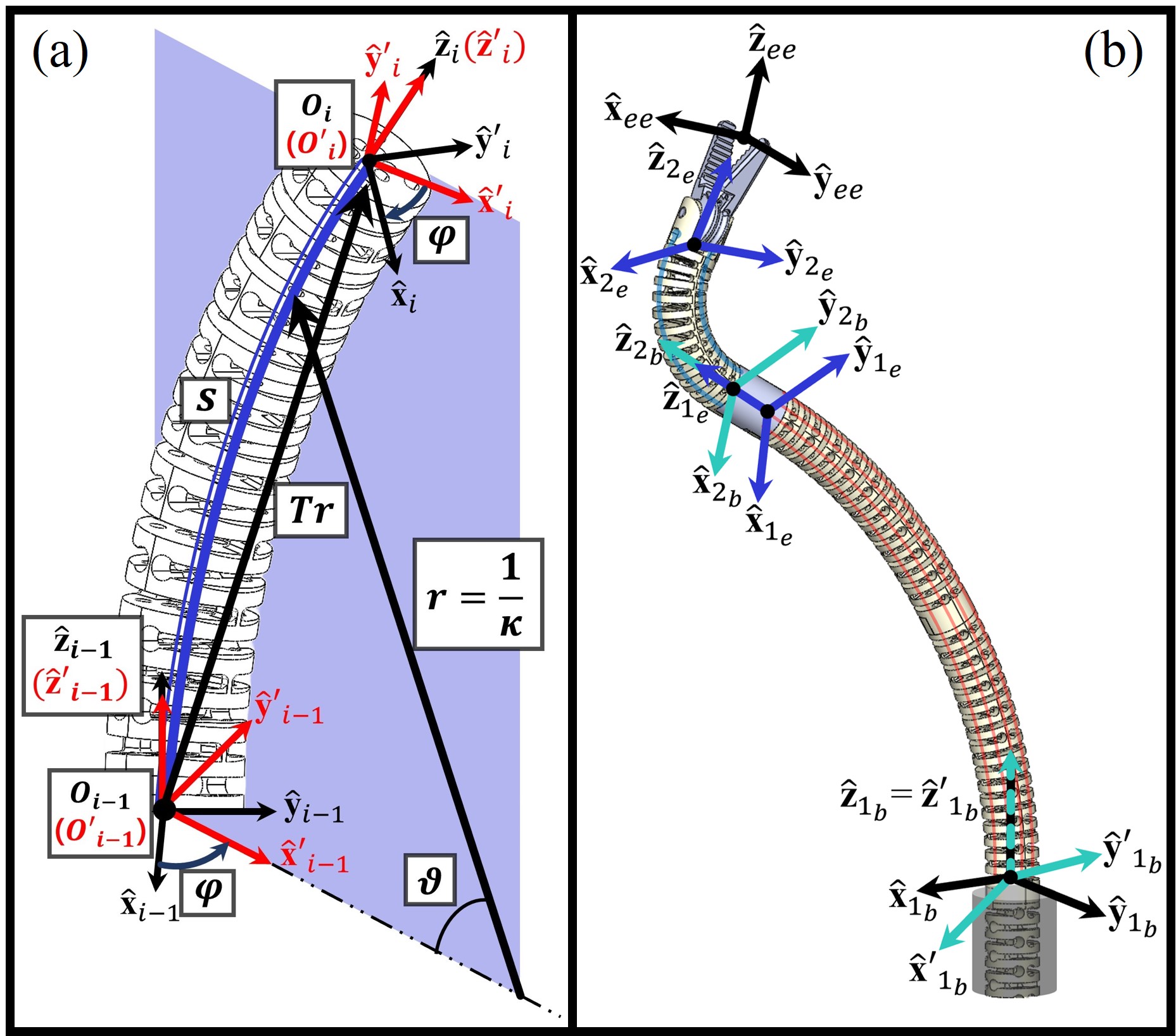
Figure 4: Kinematics diagram of a extensible segment and the proposed manipulator : (a) The coordinate frame and terminology of the extensible segment, (b) The coordinate frame and terminology of the proposed manipulator.

$${}^{1_{b}}\textrm{T}_{1^{\prime}_{b}}=\begin{bmatrix}R_{z}\left(q_{2}\right)&0\\ 0&1\end{bmatrix}$$ (6)

The transformation matrix from $O^{\prime}_{1_{b}}$ to $O_{1_{e}}$ is identical to the result of the extensible segment’s forward kinematics:

$${}^{1^{\prime}_{b}}\textrm{T}_{1_{e}}\equiv\>^{i-1}\textrm{T}_{1}$$ (7)

The transformation matrix from $O_{1_{e}}$ to $O_{2_{b}}$ applies connector length along the z-axis direction. The transformation matrix from $O_{2_{b}}$ to $O_{2_{e}}$ applies the position and rotation of segment 2, bent in the pitch direction, consistent with the assumptions of the extensible segment’s kinematics modeling. The expression for the transformation matrix is as follows:

$${}^{2_{b}}\textrm{T}_{2_{e}}=\begin{bmatrix}R_{y}\left(q_{5}\right)&P(s_{2})\\ 0&1\end{bmatrix}$$

$$\text{where}\;\;P\left(s_{2}\right)=\begin{bmatrix}\dfrac{s_{2}}{q_{5}}(1-cos(q_{5}))\\ 0\\ \dfrac{s_{2}}{q_{5}}(sin(q_{5}))\end{bmatrix}$$ (8)

The transformation matrix from $O_{2_{e}}$ to $O_{ee}$ applies yaw rotation of the forceps and length, resulting in:

$${}^{2_{e}}\textrm{T}_{ee}=\begin{bmatrix}I&a_{3}\\ 0&1\end{bmatrix}\begin{bmatrix}R_{x}\left(q_{6}\right)&{}^{2_{e}}P_{ee}\\ 0&1\end{bmatrix}$$

$$\text{where}\;\;^{2_{e}}P_{ee}=\begin{bmatrix}0\\ -sin(q_{6})d_{4}\\ cos(q_{6})d_{4}\end{bmatrix},P(s)=\left[\>0\;\;\;0\;\;\;l_{1}\>\right]^{T}$$ (9)

Finally, the transformation matrix from the manipulator’s base to the EE is obtained as follows:

$${}^{base}\textrm{T}_{ee}=^{1_{b}}\textrm{T}_{1^{\prime}_{b}}\cdot^{1^{\prime}_{b}}\textrm{T}_{1_{e}}\cdot^{1_{e}}\textrm{T}_{2_{b}}\cdot^{2_{b}}\textrm{T}_{2_{e}}\cdot^{2_{e}}\textrm{T}_{ee}$$ (10)

Specific descriptions of the proposed manipulator’s operational parameters are provided in Table I. As illustrated in Fig. 5 (b), we employ forward kinematics to compute the manipulator’s workspace, delineating reachable and unreachable areas.

To find the solution for inverse kinematics, we apply the Broyden-Fletcher-Goldfarb-Shanno Algorithm (BFGS) to obtain a numerical solution. The equation is as follows:

$$q_{k+1}=q_{k}-\alpha_{k}H_{k}J_{k}$$

$$\underset{\mathbf{q}\in\mathbb{R}^{6}}{\text{minimize}}\>f(\mathbf{q}),\>\>\>\text{where}\>f:\mathbb{R}^{6}\rightarrow\mathbb{R}$$ (11)

$$f(\mathbf{q})=\left\|T(\mathbf{q})-T_{d}\right\|$$ (12)

Here, the subscript $k$ denotes the corresponding sequence, $q$ is the joint angle, $\alpha$ is the step size, $J_{k}$ is the Jacobian matrix, $H_{k}$ is the approximated Hessian matrix, $\mathbf{q}$ represents a vector of joint angles, including $\left\{q_{1},q_{2},q_{3},q_{4},q_{5},q_{6}\right\}$, and $T(\mathbf{q})$ represents the position and orientation of Tool Center Point (TCP), and $T_{d}$ represents the desired TCP position and orientation. The $\left\|\cdot\right\|$ denotes the norm representing the magnitude of the vector.

By minimizing $f(\mathbf{q})$, one can adjust the joint angles to move the robot to the desired target position and orientation, solving the inverse kinematics problem.

III-D Workspace Comparison with Conventional Continuum Manipulator

We calculate the workspace volumes of a continuum manipulator by using the discrete integration of Tomas Simpson method [32]. We compare the workspace volumes of the proposed manipulator and a general manipulator based on the results of forward kinematics (refer to Table II and Fig. 5 (a)). When the protrusion length $q_{1}$ is at its maximum of 125mm, the volume of reachable workspace of the general continuum manipulator is $456,083\,\text{mm}^{3}$, whereas the volume of the reachable workspace of the proposed manipulator increase to $7,790,518\,\text{mm}^{3}$. The total volume of the workspace including translation is $1,496,967\,\text{mm}^{3}$ for the general continuum manipulator and $7,790,518\,\text{mm}^{3}$ for the proposed continuum manipulator. As shown in Fig. 5 (b), the volume of the accessible workspace excluding the unreachable workspace is $7,485,460\,\text{mm}^{3}$ for the proposed continuum manipulator and $1,191,909\,\text{mm}^{3}$ for the general continuum manipulator. This indicates that the presence of SAM increases the workspace volume by about 527.6%. This implies that in future surgical applications, the proposed surgical instrument by itself can access various lesions.

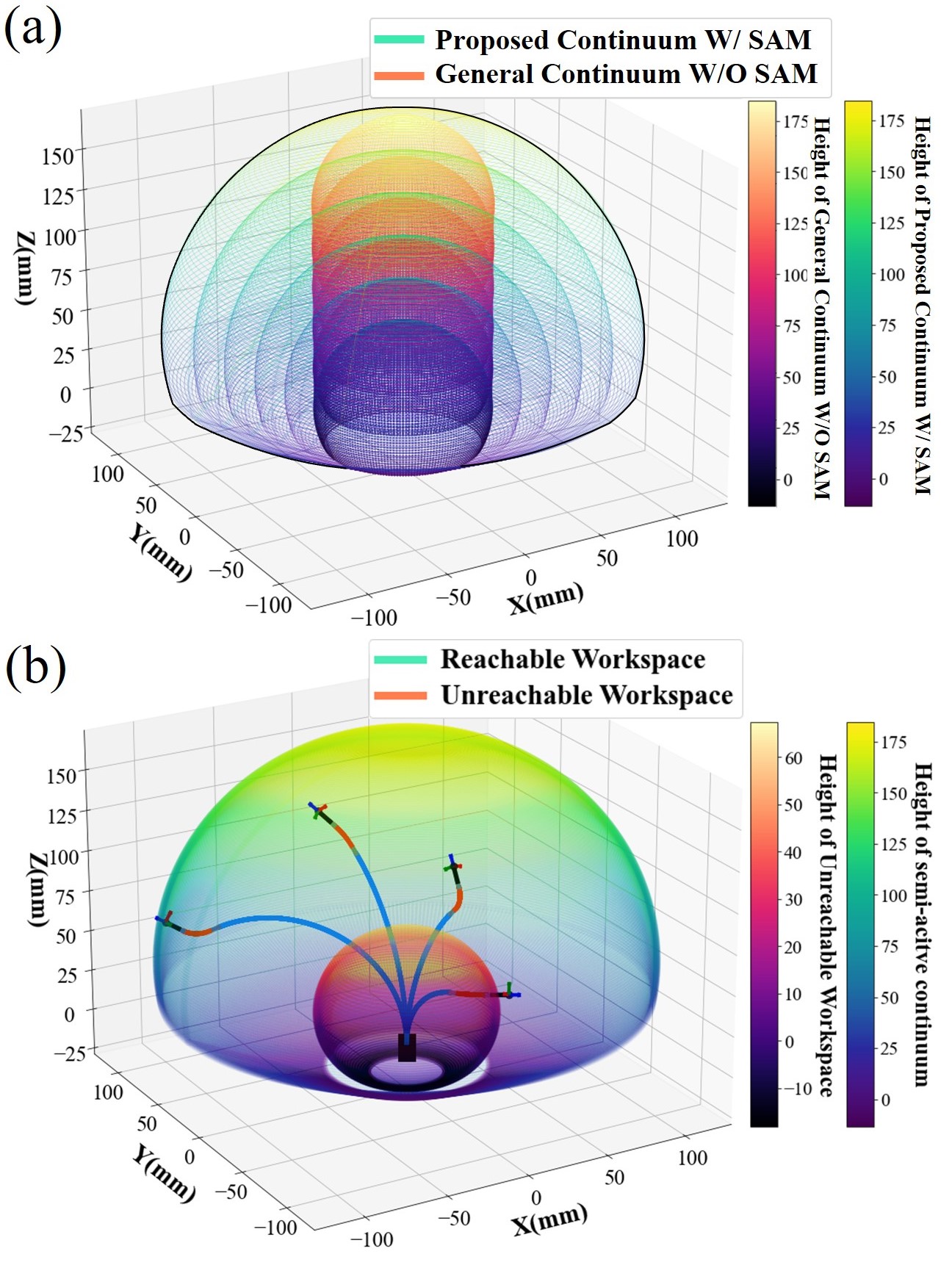
Figure 5: Visualization of the workspace of a continuum manipulator with a SAM: (a) Difference in workspace between the general continuum manipulator W/O SAM and proposed continuum manipulator W/ SAM based on translation length, (b) The reachable and unreachable workspace of the proposed manipulator W/ SAM.

TABLE II: Volume of workspace by translation, $q_{1}$

Volume     ($\times 10^{5}\,\text{mm}^{3}$)	$q_{1}$(mm)
	0	25	50	75	100	125
Semi-active	4.56	10.76	20.24	34.05	53.0	77.9
General	$\hskip 25.00003pt4.56\hskip 25.00003pt$

III-E Cable Actuation Equation

The proposed continuum manipulator is consisted with driving parts with 7 actuators, 1.5m length of insertion tube (e.g., connected cables), and proposed SAM manipulator as refer to Fig. 6. The driving part of the proposed manipulator employs $n$-type actuator, where $n$ represents the number of DOFs [33]. In this actuator, two cables are tied to a single motor, which makes it difficult to adjust cable pretension due to their coupling, compared to $2n$-type actuators. We have formulated the amount of cable length required for driving our proposed manipulator. The formula is as follows:

$$\Delta w_{i}(\vartheta_{i},d_{i})=\left(\frac{L\cdot h}{\vartheta_{i}}-\frac{d_{i}}{2}\right)\cdot 2\cdot\sin\frac{\vartheta_{i}}{2h}$$

($$i=1,\ldots,h$$) (13)

Here, $\Delta w_{i}$ represents the variation in cable length, $d_{i}$ is the diameter of segment, $L$ is the length between hinges, $\vartheta_{i}$ is the angle at which each hinge of segment bends, and $h$ is the total number of hinges.

IV Hysteresis Analysis and Compensation

Using an RGBD camera and attached fiducial markers, we obtain the measured physical joint angles ($\textbf{q}_{\mathrm{phy}}$) corresponding to the commanded joint angles ($\textbf{q}_{\mathrm{cmd}}$). Through the collected dataset, we trained TCN to model the hysteresis. The trained TCN model estimates the command joint angles ($\textbf{q}_{\mathrm{cmd}}$) based on the inputted physical joint angles ($\textbf{q}_{\mathrm{phy}}$). Leveraging the trained TCN models, we propose a hysteresis compensation control strategy to achieve more precise control of the manipulator.

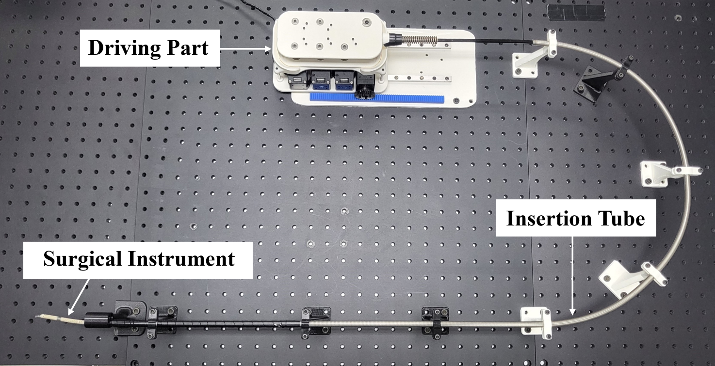
Figure 6: Robot Hardware Configuration of the proposed continuum manipulator : The main components consist of 3 parts: the driving part, insertion tube, and surgical instrument, with a total length of approximately 1.5m.

IV-A Estimation of Physical Joint Configuration

We utilize eight fiducial markers and two RGBD cameras to detect the physical joint angles. As shown in Fig. 8, we employ HSV thresholding to identify each marker and obtain its corresponding point cloud data. The RANSAC algorithm [34] is then applied to estimate the center of each marker. The base pose of the manipulator is calculated using the following equations:

$${}^{cam}\hat{\textbf{x}}_{base}=^{cam}\hat{\textbf{y}}_{base}\crossproduct^{cam}\hat{\textbf{z}}_{base}$$

$${}^{cam}\hat{\textbf{y}}_{base}=(^{cam}\textbf{p}_{r_{0}}-^{cam}\textbf{p}_{r_{1}})/\norm{{}^{cam}\textbf{p}_{r_{0}}-^{cam}\textbf{p}_{r_{1}}}$$

$${}^{cam}\hat{\textbf{z}}_{base}=(^{cam}\textbf{p}_{r_{1}}-^{cam}\textbf{p}_{b_{0}})/\norm{{}^{cam}\textbf{p}_{r_{1}}-^{cam}\textbf{p}_{b_{0}}}$$

$${}^{cam}\textbf{p}_{base}=(^{cam}\textbf{p}_{r_{0}}+^{cam}\textbf{p}_{b_{0}})/2+\textbf{p}_{offset}$$ (14)

where ${}^{cam}\hat{\textbf{x}}_{base}$, ${}^{cam}\hat{\textbf{y}}_{base}$, and ${}^{cam}\hat{\textbf{z}}_{base}$ are the unit vectors of the robot base frame in the camera frame. ${}^{cam}\textbf{p}_{r_{0}}$, ${}^{cam}\textbf{p}_{r_{1}}$, and ${}^{cam}\textbf{p}_{b_{0}}$ denote the center positions of red ball 0, red ball 1, and blue ball 0 in the camera frame (see Fig. 8 for marker index information). $\textbf{p}_{offset}$ is the fixed offset between the manipulator base and the base markers, determined from design parameters.

The EE pose detection is described in Fig. 7. To address potential marker occlusion during data collection, we use five markers instead of the minimum three required to determine the EE pose.

The transformation matrix from the base frame to the EE frame (${}^{base}T_{ee}$) is estimated using the obtained camera-to-base (${}^{cam}T_{base}$) and camera-to-EE (${}^{cam}T_{ee}$) transformation matrices:

$${}^{base}T_{ee}=\>^{cam}T_{base}^{-1}\cdot^{cam}T_{ee}$$ (15)

With the computed ${}^{base}T_{ee}$ matrix, we can solve the inverse kinematics (detailed in Section III-C) to obtain the physical joint angles ($\textbf{q}_{\mathrm{phy}}$).

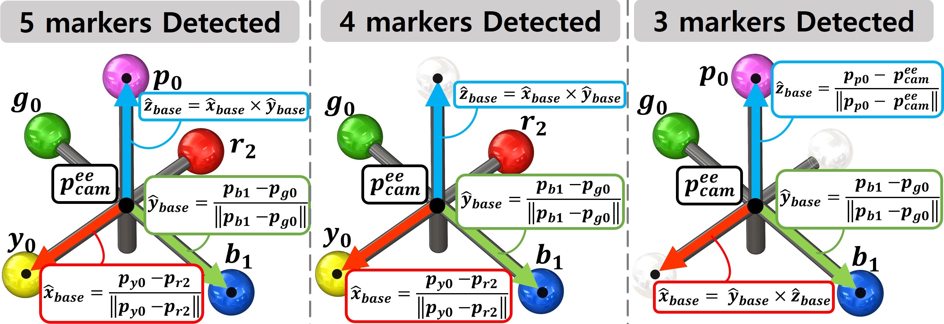
Figure 7: Pose estimation of manipulator’s EE using 5 fiducial markers: This figure illustrates the method used to estimate the relative pose (position and orientation) of the camera frame with respect to the manipulator’s end-effector (EE) using five fiducial markers. Three scenarios are considered: (1) All five markers are detected. (2) Four markers are visible due to occlusion. (4 different configurations exist depending on the occluded markers.) (3) Three markers are detected due to occlusion. (total of 10 different configurations exist). For scenarios with partial occlusion (cases 2 and 3), the approach involves obtaining the 3D coordinates (denoted by $\textbf{p}^{EE}_{cam}$) of the EE center in the camera frame using the detected markers. This then allows for calculating the end-effector frame.

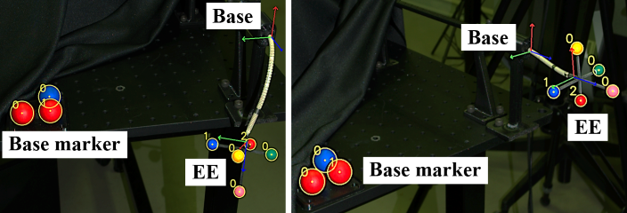
Figure 8: Physical joint angle estimation: Using 8 fiduical markers and RGBD camera, we obtain the transformation matrix of cam to base (${}^{cam}T_{base}$), and cam to EE (${}^{cam}T_{EE}$).

IV-B Data Collection and Hysteresis Analysis

Building upon the physical joint angles obtained in Section IV-A, we investigate how translation affects the hysteresis behavior of the proposed continuum manipulator. As translation increases, the activated length of segment 1 grows, leading to decreased stiffness. This results in greater deflection for the same driving moment applied at the joints.

To analyze this effect, we generated a set of random trajectories (denoted by $\mathcal{D}_{trans_{i}}$). Within each trajectory, the command joint angles for joints $q_{2}$ to $q_{7}$ are identical. These angles are randomly chosen within specific ranges for each joint (i.e., $q_{2}$: $[-30^{\circ},30^{\circ}$], $q_{3}$ to $q_{5}$ : $[-60^{\circ},60^{\circ}]$, $q_{6}$ to $q_{7}$ = $0^{\circ}$).

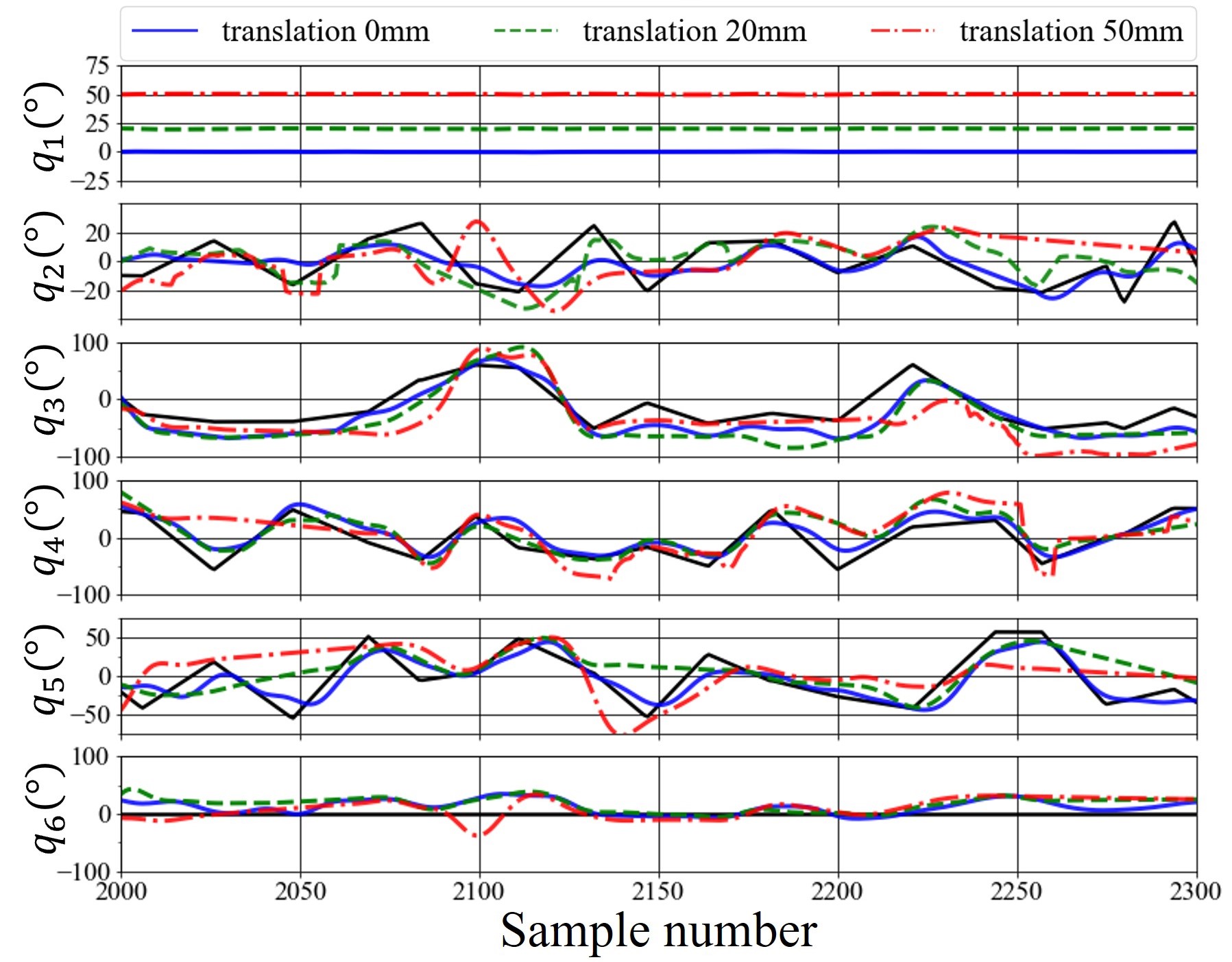
Figure 9: The comparision of the command and the physical joint angles through the collected $\mathcal{D}$: The X-axis represents the sample number during the measurement process. The Y-axis represents the joint angle (in degrees) for each joint of the SAM instrument (denoted as $q_{1}$, $q_{2}$, …, $q_{6}$). The black line states the $\textbf{q}_{\mathrm{cmd}}$. The blue, green, and red dashed lines represent the measured physical joint angles ($\textbf{q}_{\mathrm{phy}}$) on 0mm, 20mm, 50mm translations, respectively. The difference between $\textbf{q}_{\mathrm{cmd}}$ and $\textbf{q}_{\mathrm{phy}}$ illustrates the hysteresis effect.

TABLE III: Hysteresis statics on different translation

Trans	Error	$q_{1}$ [mm]	$q_{2}$ [∘]	$q_{3}$ [∘]	$q_{4}$ [∘]	$q_{5}$ [∘]	$q_{6}$ [∘]
0mm	MAE	0.1	8.2	18.1	11.9	10.3	19.0
	SD	0.1	6.0	12.0	9.1	7.4	12.8
	MSE	0.0	1.0	15.3	-7.7	-0.1	-17.4
	SD	0.1	10.1	15.4	12.9	12.7	14.8
20mm	MAE	0.1	11.2	28.4	18.3	12.6	19.6
	SD	0.1	7.9	16.5	12.4	9.4	13.5
	MSE	0.0	0.1	25.7	-9.2	-5.6	-17.9
	SD	0.2	13.7	20.4	20.1	14.7	15.7
50mm	MAE	0.1	15.1	46.4	30.0	21.7	23.1
	SD	0.1	10.7	24.9	19.8	15.3	16.0
	MSE	0.0	-0.1	42.1	-10.8	-16.4	-17.8
	SD	0.1	18.5	31.6	34.3	20.9	21.7

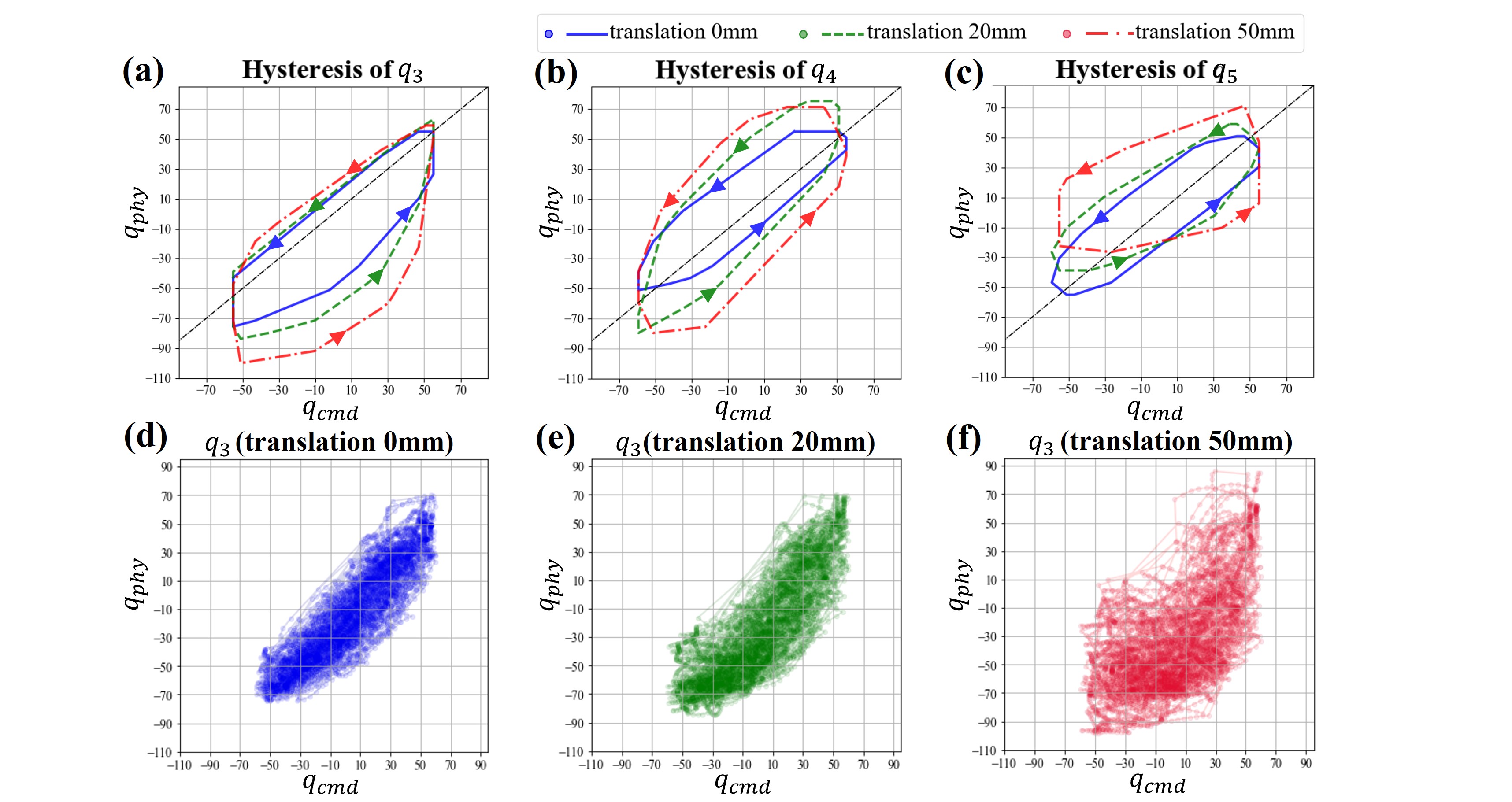
Figure 10: Hysteresis loop on different translation: This figure depicts the hysteresis loop of the proposed Semi-Active Segment (SAM) instrument at different extension levels (translation lengths). The blue, green, and red color states translation 0 mm, 20 mm, and 50 mm, respectively. (a), (b), (c) states the outermost points of the hysteresis loop on $q_{3}$, $q_{4}$, $q_{5}$, respectively. On (a), (b), (c), the black dashed line represent the reference line. (d), (e), and (f) states the hysteresis loop on $q_{3}$ on different translations, and each figure plotted utilizing collected dataset, $\mathcal{D}$. Notice that the $q_{3}$ exhibit a wider variation as the extension level increases. The proposed SAM mechanisms exhibits different nonlinear hysteresis on different extension levels and higher extension levels lead to a larger discrepancy between commanded and achieved joint angles. This characteristics makes it hard to model the hysteresis of SAM mechanism.

The translation value ($q_{1}$) varies between trajectories, represented by the subscript $i$ in $\mathcal{D}_{trans_{i}}$. Each command joint angle is linearly interpolated with a step size of 3 degrees. The trajectory data is structured as follows:

$$\mathcal{D}_{trans_{i}}=\{\textbf{q}_{\mathrm{cmd}},\textbf{q}_{\mathrm{phy}}\}_{1}^{N}$$

$$\mathcal{D}=\{\mathcal{D}_{trans_{i}}|(i=0,10,20,30,40,50)\}$$ (16)

• $\mathcal{D}_{trans_{i}}$ : This dataset stores pairs of corresponding command joint angles ($\textbf{q}_{\mathrm{cmd}}$) and physical joint angles ($\textbf{q}_{\mathrm{phy}}$) for $N$ data points.

• $\mathcal{D}$ : This dataset combines multiple $\mathcal{D}_{trans_{i}}$ datasets for different translation values ($i$ = 0, 10, 20, 30, 40, 50 mm).

We analyzed the translation-induced hysteresis using the collected dataset $\mathcal{D}$ ($N$ = 4,955, total: 29,730). Detailed statistics and figures of $\mathcal{D}$ are presented in Fig. 9 and Table III. The analysis revealed a trend: as the translation distance increases, the Mean Absolute Error (MAE, (17) of joint angles $q_{3}$ and $q_{4}$ (corresponding to the pitch and yaw directions of extensible segment 1) also grow significantly. Fig. 10 shows the hysteresis loop widening with increasing extension levels. Higher extension leads to lower structural stiffness, resulting in larger deflections of the manipulator even under the same cable-driven moment.

$$MAE=\frac{1}{n}\sum_{i=1}^{n}\>{|\textbf{q}_{\mathrm{phy}}-\textbf{q}_{\mathrm{cmd}}|}$$ (17)

$$MSE=\frac{1}{n}\sum_{i=1}^{n}\>(\textbf{q}_{\mathrm{phy}}-\textbf{q}_{\mathrm{cmd}})$$ (18)

Furthermore, $q_{3}$ exhibited biased hysteresis with a near-equal relationship between the Mean Signed Error (MSE, (18)) and MAE across various translation values (e.g., MAE/MSE of 18.1/15.3 at 0 mm, 28.4/25.7 at 25 mm, and 46.4/42.1 at 50 mm translation). As shown in Fig. 10-(a), $\textbf{q}_{\mathrm{phy}}$ consistently falls below the reference line across all $\textbf{q}_{\mathrm{cmd}}$ values. This bias stems from the inherent difficulty of $n$-type actuators in maintaining equal initial tension in antagonistic cable pairs. The initial tension imbalance is amplified by larger translations, which reduce structural stiffness, resulting in higher deflections at greater extension levels. We infer that the cable driving positive $q_{3}$ likely has a higher initial tension than its negative counterpart, contributing to this observed bias.

IV-C Hysteresis Modeling using Deep Learning

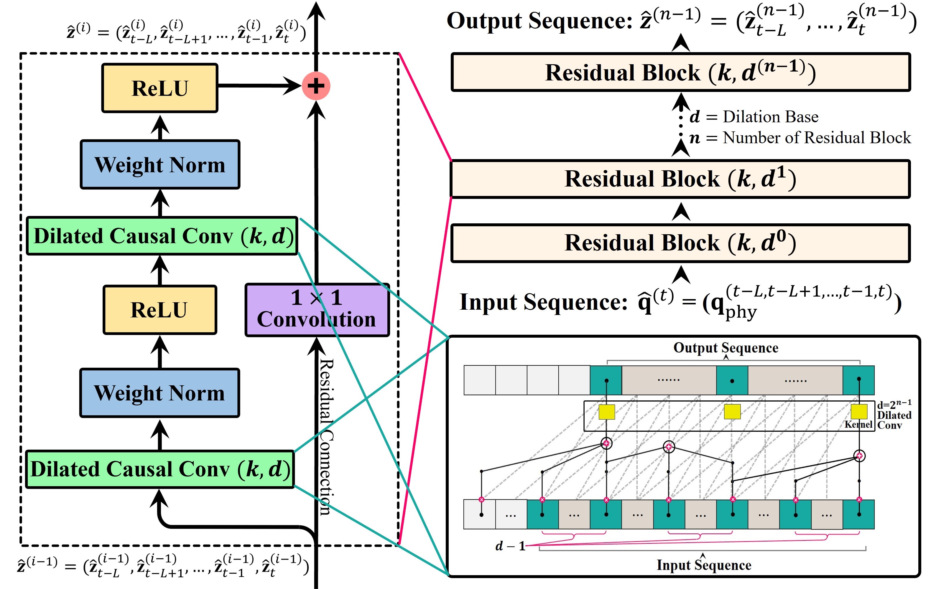
Figure 11: Architecture of TCN: TCN composed with layers of 1D dilated convolution layer, which can get features from the history of the joints. The dilation base was set as $2$, so the dilation factor is increase in $2^{0}$, $2^{1}$, …, and $2^{i}$. The last of the feature vector, $\hat{z}_{L}^{t}$, become the outputs of the model.

We employed a TCN [35] for hysteresis estimation due to its proven effectiveness in this domain. As detailed in [30], TCN efficiently compensate for the hysteresis effect. The TCN architecture consists of serially connected residual blocks. Each residual block incorporates two dilated convolutions, two weight normalization layers, and two ReLU activation functions (refer to Fig. 11 for details). The residual blocks employ exponentially increasing dilation factors with a base of 2 ($d$). The first residual block has dilation factor of $1$($2^{0}$), the second residual block has dilation factor of $2$ ($2^{1}$), and others has $2^{n-1}$ dilation factor. The number of residual blocks ($n$) are determined by the (19). In (19), the $L$ is the input sequence length and $k$ is kernel size. In our setting, the kernel size is 3. The TCN returns the feature vectors of the input sequence ($\hat{\textbf{z}}^{(n-1)}$). The last one of the feature vector ($\hat{\textbf{z}}_{t}^{(n-1)}$) serving as the estimated $\textbf{q}_{\mathrm{cmd}}$ corresponding to the input $\textbf{q}_{\mathrm{phy}}$ as refer to (20).

$$num\>block=\lceil\log_{2}\frac{(L-1)}{2k-2}+1\rceil$$ (19)

$$\hat{\textbf{q}}_{\mathrm{cmd}}^{(t)}=\hat{\textbf{z}}_{t}^{(n-1)}=f_{\theta}(\textbf{q}_{\mathrm{phy}}^{(t-L,\>t-L+1,\>...,\>t-1,\>t)})$$ (20)

For training the TCN models, we utilize a dataset, $\mathcal{D}_{train}$, containing 4,955 randomly commanded joint angles across 6 different translations, resulting in a total of 29,730 data points. Validation datasets, $\mathcal{D}_{valid}$, are employed, each containing 1,307 command joint angles across 6 translations, totaling 7,842 data points.

TABLE IV: Performance comparison of TCN-inverse models for each sequence length, $L$ on test dataset

MAE / L	$L=10$	$L=50$	$L=100$	$L=150$
Model 1 $[MAE\pm SD]$	$5.5\pm 8.3$	$7.6\pm 10.3$	$8.3\pm 11.0$	$8.5\pm 11.1$
Model 2 $[MAE\pm SD]$	$5.6\pm 8.3$	$8.1\pm 11.9$	$8.8\pm 12.0$	$9.7\pm 12.7$
Model 3 $[MAE\pm SD]$	$5.6\pm 8.4$	$8.6\pm 11.8$	$9.0\pm 12.0$	$9.8\pm 13.3$

To mitigate biases from random weight initialization, each TCN model is trained three times with varying initial weights. Additionally, we investigate the impact of different input sequence lengths ($L$ = 10, 50, 100, 150) and determine the optimal input sequence length which can capture the history-dependent hysteresis in continuum manipulators.

During training, we use a fixed learning rate of 0.001, mean squared error as the loss function, and utilization of Adam optimizer. After 10,000 epochs, the model with the lowest validation loss from each training phase is selected. These optimal models are then evaluated on unseen trajectories from the test dataset ($\mathcal{D}_{test}$).

As detailed in Table IV (e.g., Mean Absolute Error (MAE) and Standard Deviation (SD)), the TCN model with a sequence length ($L$) of 10 achieve the best performance, exhibiting lower MAE and SD compared to other lengths. This suggests that a memory of the past 10 timesteps is sufficient for the model to effectively capture the hysteresis behavior.

IV-D Design of Hysteresis Compensation Algorithm

In this section, we present the design of the proposed hysteresis compensation algorithm, which leverages three TCN with input sequence length $L=10$. These models achieved the best performance on the test dataset, as detailed in Section  IV-C. Hysteresis compensation aims to return calibrated command joint angles that can accurately reach the inputted desired joint angles.

The trained TCN models (refer to (20)) predict command joint angles for given physical joint angles. Consequently, the predicted command joint angles corresponding to the desired joint angles can be directly input into the control algorithm. Our proposed hysteresis compensation control algorithm exclusively employs TCN models. These models receive a sequence of desired joint angles ($\textbf{q}_{\mathrm{desired}}$) as input and output the corresponding calibrated commanded joint angles ($\textbf{q}_{\mathrm{cal}}$).

As shown in Algorithm 1 and Fig. 12, the calibrated command joint angle ($\hat{\textbf{q}}_{\mathrm{cal}}^{(t)}$) is computed as the average of outputs from three individual TCN models ($\hat{\textbf{q}}_{\mathrm{cal_{1}}}^{(t)}$, $\hat{\textbf{q}}_{\mathrm{cal_{2}}}^{(t)}$, $\hat{\textbf{q}}_{\mathrm{cal_{3}}}^{(t)}$). This ensemble approach aims to enhance output stability. Due to random weight initialization, the three models exhibit some variance even with identical inputs. Averaging their outputs mitigates this effect and improves accuracy. The proposed algorithm achieves a time latency of 1ms, ensuring real-time control capabilities.

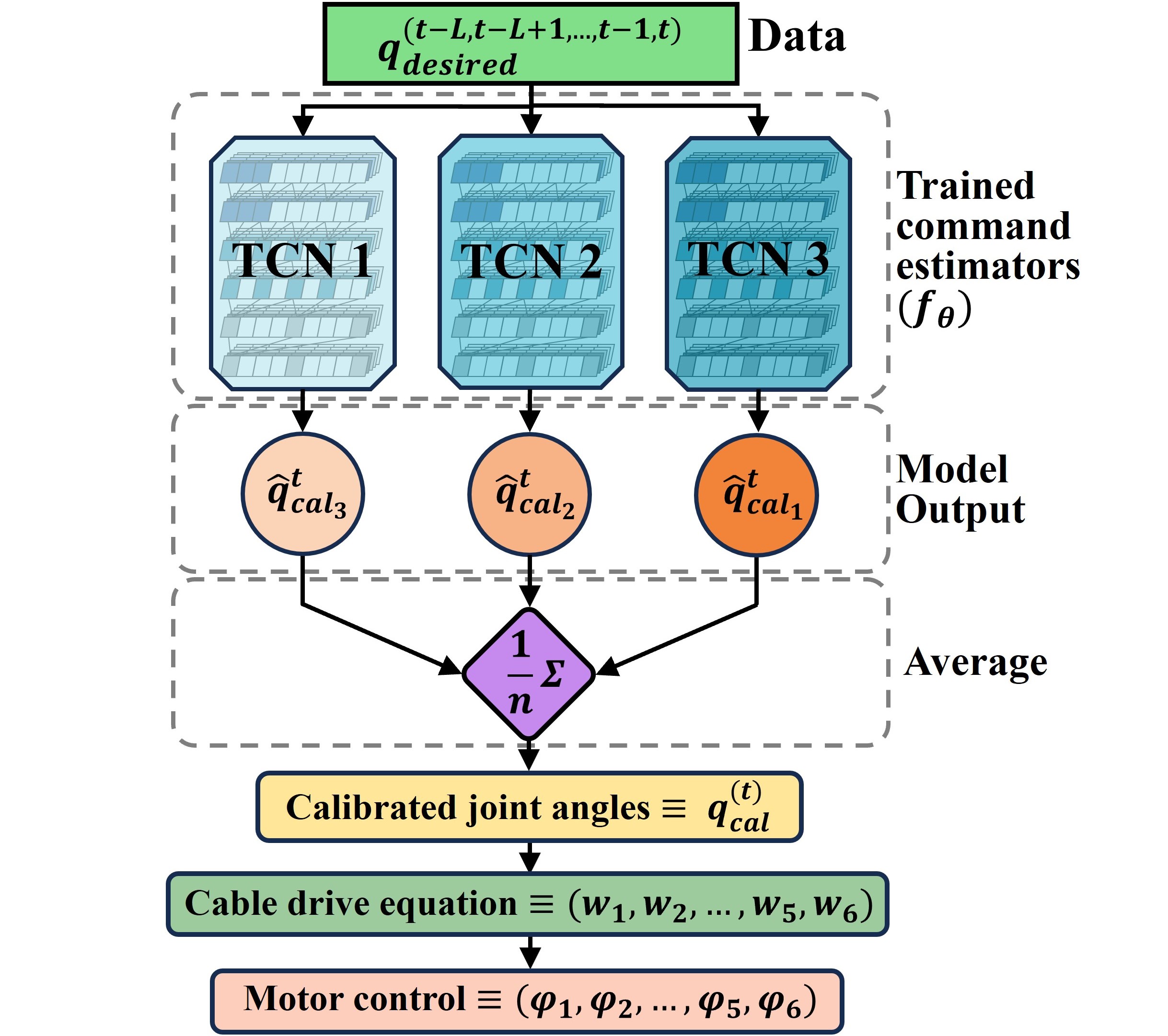
Figure 12: Hysteresis Compensation Control Method: Using the trained TCN models, we get the output, $\hat{\textbf{q}}_{cal_{1,2,3}}^{(t)}$, on the desired joint angle. Then, we get average of the $\hat{\textbf{q}}_{cal_{1,2,3}}^{(t)}$, to obtain the final calibrated joint angle ($\hat{\textbf{q}}_{cal}$).

V Results and Validation

This section evaluates the performance of the calibrated controller in comparison to the uncalibrated controller.

• Calibrated Controller: The desired joint angles ($\textbf{q}_{\mathrm{desired}}$) serve as input. The calibrated command joint angles ($\textbf{q}_{\mathrm{cal}}$) for achieving $\textbf{q}_{\mathrm{desired}}$ are computed by processing them through the three trained TCN models (as described in Section IV-D). Subsequently, the motor commands for $\textbf{q}_{\mathrm{desired}}$ are calculated using equation (13).

• Uncalibrated Controller: The desired joint angles are directly input into the control equation (equation (13)).

The validation process comprises two distinct tasks: a random trajectory tracking test and a box pointing task. These tasks are designed to assess the accuracy of the calibrated control in both joint space (via the random trajectory tracking test in Section V-A) and operational space (via the box pointing task in Fig. 14).

V-A Random Trajectory Tracking Test

This section compares the performance of the uncalibrated and calibrated controllers in tracking random joint space trajectories. It’s important to note that the training data in Section IV-C included translations at $0$, $10$, $20$, $30$, $40$, and $50mm$. To test generalization, random trajectories are generated for unseen translations: $5mm$, $25mm$, and $45mm$.

For joints $q_{3}$ to $q_{5}$, values are randomly assigned within the range $[-60^{\circ},:60^{\circ}]$, while for $q_{2}$, values are randomly assigned within $[-30^{\circ},:30^{\circ}]$. Each trajectory comprises 955, 887, and 941 desired joint angles ($\textbf{q}_{\mathrm{desired}}$) respectively, with each angle linearly interpolated by 3 degrees.

We obtained the physical joint angles for both the uncalibrated and calibrated controllers using an RGBD camera and 8 fiducial markers (employing the same methods as in Section IV-A), with $\textbf{q}_{\mathrm{desired}}$ as input. The results for physical joint angles of each controller are detailed in Fig. 13 for the three trajectories (translations: $5mm$, $25mm$, and $45mm$). The proposed calibrated controller effectively mitigates hysteresis effects, consistently demonstrating lower Mean Absolute Error (MAE) across all joints compared to the uncalibrated controller (refer to Fig. 13 and Table V). Notably, these significant improvements are achieved even with unseen translations, highlighting the generalizability of the compensation method beyond the specific training data. The summary of the notable observed reductions in MAE is as follows:

• Translation 5 mm: $q_{3}$, $q_{4}$, $q_{5}$ exhibit reductions of 69.5 %, 46.8 %, and 33.0 %, respectively.

• Translation 25 mm: $q_{3}$, $q_{4}$, $q_{5}$ exhibit reductions of 53.2%, 56.5%, and 29.9%, respectively.

• Translation 45 mm: $q_{3}$, $q_{4}$, $q_{5}$ exhibit reductions of 57.7%, 40.2%, and 54.1%, respectively.

Algorithm 1 Hysteresis Compensation Algorithm

0:  Sequence of desired joint angles $\textbf{q}_{desired}^{t,...,t-M}$ $(M\leq L)$, command estimators $f_{\theta_{1}}$, $f_{\theta_{2}}$, and $f_{\theta_{3}}$, time sequence length $L$

1:  if $M$ $<$ $L$ then

2:     $\textbf{q}_{desired}^{t-M-1},...,\textbf{q}_{desired}^{t-L}$ $\leftarrow zero$ $padding$

3:  end if

4:  $\hat{\textbf{q}}_{cal_{1,2,3}}^{(t)}=f_{\theta_{1,2,3}}(\textbf{q}_{desired}^{(t)},...,\textbf{q}_{desired}^{(t-L)})$

5:  $\textbf{q}_{\mathrm{cal}}^{(t)}=(\hat{\textbf{q}}_{\mathrm{cal_{1}}}^{(t)}+\hat{\textbf{q}}_{\mathrm{cal_{2}}}^{(t)}+\hat{\textbf{q}}_{\mathrm{cal_{3}}}^{(t)})/3$

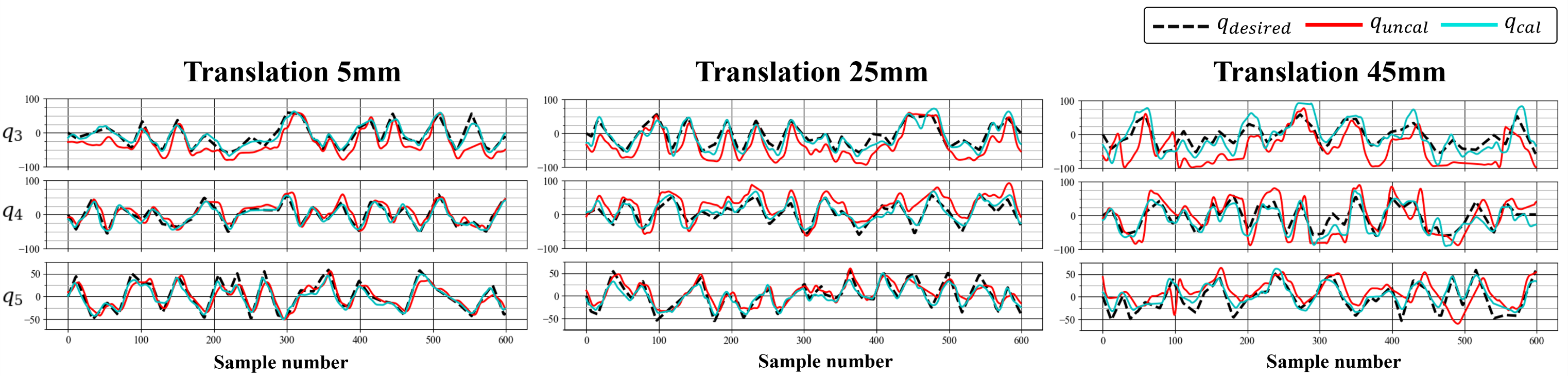
Figure 13: Performance comparison of calibrated and uncalibrated controller on random trajectory tracking test using three unseen trajectory: This figure compares the performance of a calibrated controller (blue line, $\textbf{q}_{\mathrm{cal}}$ ) and an uncalibrated controller (red line, $\textbf{q}_{\mathrm{uncal}}$ ) on a random trajectory tracking test using three unseen trajectories (not previously encountered by the controllers). The black dashed line represents the desired trajectory ($\textbf{q}_{\mathrm{desired}}$ ). The calibrated controller shows significantly better tracking performance, following the desired trajectory more closely compared to the uncalibrated controller. This highlights the effectiveness of the calibration process in improving the accuracy of the manipulator’s movements.

TABLE V: Performance Comparison between Uncalibrated and Calibrated Control on Random Trajectory Tracking Test

Trans / MAE		Translation 5 mm					Translation 25 mm					Translation 45 mm
		$q_{2}$	$q_{3}$	$q_{4}$	$q_{5}$	$q_{6}$	$q_{2}$	$q_{3}$	$q_{4}$	$q_{5}$	$q_{6}$	$q_{2}$	$q_{3}$	$q_{4}$	$q_{5}$	$q_{6}$
Caibrated	MAE	4.2	6.8	6.6	6.3	14.2	8.5	14.6	11.0	7.5	17.0	12.2	18.3	17.7	9.5	16.3
	SD	3.1	5.4	5.2	5.1	9.2	6.1	11.9	8.3	5.7	11.7	8.2	13.8	12.6	7.7	12.3
Uncalibrated	MAE	8.9	22.3	12.4	9.4	19.7	13.3	31.2	25.3	10.7	24.6	15.5	43.3	29.6	20.7	26.7
	SD	6.0	14.7	9.3	6.7	11.4	8.9	16.4	14.6	8.3	14.9	10.6	23.8	19.6	15.2	18.1
* MAE represents that mean absolute error.

V-B Box Pointing Task

This section assesses the effectiveness of the proposed hysteresis compensation method in achieving accurate positioning. The experiment utilizes five boxes of varying heights, each attached with unique red, green, and blue fiducial markers (refer to Fig. 14).

An RGBD camera captures the markers, enabling the estimation of their centers using the methods described in Section IV-A. These marker positions are then used to compute the transformation matrix from the camera frame to each box frame ${}^{cam}T_{box_{j}}$ $(j=1,2,3,4,5)$ using Equation (18):

$${}^{cam}\hat{\textbf{x}}_{box_{j}}=^{cam}\hat{\textbf{y}}_{box_{j}}\crossproduct^{cam}\hat{\textbf{z}}_{box_{j}}$$

$${}^{cam}\hat{\textbf{y}}_{box_{j}}=(^{cam}\textbf{p}_{r_{j}}-^{cam}\textbf{p}_{g_{j}})/\norm{{}^{cam}\textbf{p}_{r_{j}}-^{cam}\textbf{p}_{g_{j}}}$$

$${}^{cam}\hat{\textbf{z}}_{box_{j}}=(^{cam}\textbf{p}_{r_{j}}-^{cam}\textbf{p}_{b_{j}})/\norm{{}^{cam}\textbf{p}_{r_{j}}-^{cam}\textbf{p}_{b_{j}}}$$

$${}^{cam}\textbf{p}_{box_{j}}=(^{cam}\textbf{p}_{g_{j}}+^{cam}\textbf{p}_{b_{j}})/2+\textbf{p}_{x_{offset}}$$ (21)

where ${}^{cam}\textbf{p}_{r_{j}}$, ${}^{cam}\textbf{p}_{b_{j}}$, and ${}^{cam}\textbf{p}_{g_{j}}$ are the center positions (in the camera frame) of the red, blue, and green spheres on each box (denoted by subscript j), respectively. Using inverse kinematics (detailed in Section III-C), the target joint angles ($\textbf{q}_{box_{j}}$) required to reach designated points on each box are calculated through the obtained ${}^{cam}T_{box_{j}}$.

The manipulator executes a series of motions to reach target positions on each box, beginning with the lowest box and sequentially progressing to the highest. This process is repeated 15 times with the boxes placed in random configurations. Two control strategies are compared: the uncalibrated controller and the proposed calibrated controller. The position errors between the desired positions and the physical end effector’s positions are evaluated for both controllers.

The proposed calibrated controller demonstrates consistent superiority over the uncalibrated controller across all spatial dimensions ($x$, $y$, $z$) and the overall Euclidean distance. As detailed in Table VI, the calibrated controller achieves significant error reductions:

• $x:(mm)$: MAE and SD are decreased by 36.9% and 38.2%, respectively.

• $y:(mm)$: MAE and SD are decreased by 38.1% and 47.8%, respectively.

• $z:(mm)$: MAE and SD are decreased by 43.5% and 37.4%, respectively.

• Euclidean Distance: MAE and SD are decreased by 25.8% and 56.7%, respectively.

VI CONCLUSIONS

This study introduced a novel continuum manipulator incorporating SAM, enabling extended reach without increasing size or degrees of freedom. The proposed design demonstrated a significant 527.6% expansion in reachable workspace volume compared to conventional continuum manipulators. However, the instrument exhibited considerable hysteresis, primarily due to cable effects such as friction, elongation, and coupling. Moreover, the hysteresis model was observed to vary with increasing extension length, attributed to changes in structural stiffness.

To address the variation in hysteresis with extension, we proposed a real-time deep learning-based compensation control algorithm. We utilized an RGBD camera and 8 fiducial markers to collect joint angle data from the manipulator. Through collected dataset, we trained TCN models. These models estimate the command joint angles for the inputted physical joint angles. Trajectory tracking tests on unseen trajectories demonstrated significant and consistent reduction in hysteresis across all joint angles, particularly in the highly affected $q_{3}$ joint. The calibrated controller achieved substantial improvements in joint space: for translation 5mm, $q_{3}$ error was reduced from 22.3° to 6.8°; for translation 25mm, $q_{3}$ error went from 31.2° to 14.6°; and for translation 45mm, $q_{3}$ error decreased from 43.3° to 18.3°. Similarly, the box pointing task with the calibrated controller showed significant reductions in position error across all axes: $x$ (mm) error decreased from 21.09 to 13.31 (MAE), $y$ (mm) error went from 19.73 to 12.22 (MAE), $z$ (mm) error reduced from 20.04 to 11.32 (MAE), and the average Euclidean distance error decreased from 32.33mm to 23.99mm.

These results demonstrate that despite the presence of hysteresis effects, the proposed controller with TCN-based compensation effectively reduced error and deviation. Our research implies that in future surgical applications, using the proposed SAM mechanism surgical tool, we can access various lesions without accessing the overtube, which can lead to damage to surrounding tissues. Additionally, the improvement in hysteresis compensation has the potential to significantly enhance surgical task performance by minimizing position and joint angle errors in real-time.

Figure 14: Box pointing task : (a) Demonstration figure of the task: This part of the evaluation assesses the effectiveness of the End-Effector (EE) in precisely reaching randomly positioned target points (yellow) on five boxes. We compare the positioning error between the calibrated and uncalibrated control approaches. (b) and (c) visualize the difference in positioning error between the calibrated and uncalibrated controllers relative to the target points.

TABLE VI: Performance Comparision betwen Calibrated and Uncalibrated Control on Box Picking Task

EE Position Error		Calibrated Control	Uncalibrated Control
$x$ (mm)	MAE	13.31	21.09
	SD	15.19	24.57
$y$ (mm)	MAE	12.22	19.73
	SD	14.55	27.86
$z$ (mm)	MAE	11.50	20.04
	SD	14.47	23.12
Euclidean distance (mm)	AVG	23.99	32.33
	SD	9.52	21.95

VII ACKNOWLEDGEMENT

This work was supported by the DGIST R&D Program of the Ministry of Science and ICT (23-PCOE-02, 23-DPIC-20), by the DGIST Start-up Fund Program of the Ministry of Science and ICT (2024010213), and by the collaborative project with ROEN Surgical Inc. This work was supported by the Korea Medical Device Development Fund grant funded by the Korea government (Project Number: 1711196477 , RS-2023-00252244) and by the National Research Council of Science & Technology (NST) grant funded by the Korea government (MSIT) (CRC23021-000).

References

- [1] B. S. Peters et al., “Review of emerging surgical robotic technology,” Surgical endoscopy, vol. 32, pp. 1636–1655, 2018.
- [2] M. Hwang and D. Kwon, “K‐flex: a flexible robotic platform for scar‐free endoscopic surgery,” The International Journal of Medical Robotics and Computer Assisted Surgery, vol. 16, p. e2078, 2020.
- [3] M. Remacle et al., “Transoral robotic surgery (TORS) with the Medrobotics Flex™ System: first surgical application on humans,” European Archives of Oto-Rhino-Laryngology, vol. 272, pp. 1451–1455, 2015.
- [4] S. J. Phee et al., “Master and slave transluminal endoscopic robot (MASTER) for natural orifice transluminal endoscopic surgery,” in Proc. 2009 Annual International Conference of the IEEE Engineering in Medicine and Biology Society, 2009.
- [5] L. Zorn et al., “A novel telemanipulated robotic assistant for surgical endoscopy: preclinical application to ESD,” IEEE Transactions on Biomedical Engineering, vol. 65, pp. 797–808, 2017.
- [6] T. da Veiga et al., “Challenges of continuum robots in clinical context: a review,” Prog. Biomed. Eng., vol. 2, 2020.
- [7] Burgner-Kahrs, D. Jessica et al., “Continuum robots for medical applications: A survey,” IEEE Transactions on Robotics, vol. 31, pp. 1261–1280, 2015.
- [8] M. W. Gifari et al., “A review on recent advances in soft surgical robots for endoscopic applications.” The International Journal of Medical Robotics and Computer Assisted Surgery, vol. 15, p. e2010, 2019.
- [9] H. M. Le et al., “A survey on actuators-driven surgical robots,” Sensors and Actuators A: Physical, vol. 247, pp. 323–354, 2016.
- [10] M. M. Dalvand et al., “An analytical loading model for -tendon continuum robots.” IEEE Transactions on Robotics, vol. 34, pp. 1215–1225, 2018.
- [11] H. Yuan, L. Zhou et al., “A comprehensive static model of cable-driven multi-section continuum robots considering friction effect,” Mechanism and Machine Theory, vol. 135, pp. 130–149, 2019.
- [12] D. Ji et al., “Analysis of twist deformation in wire-driven continuum surgical robot,” International Journal of Control, Automation and Systems, vol. 18, pp. 10–20, 2020.
- [13] R. Roy et al., “Modeling and estimation of friction, extension, and coupling effects in multisegment continuum robots.” IEEE/ASME Transactions on Mechatronics, vol. 22, pp. 909–920, 2016.
- [14] H. Kim et al., “Effect of backlash hysteresis of surgical tool bending joints on task performance in teleoperated flexible endoscopic robot.” The International Journal of Medical Robotics and Computer Assisted Surgery, vol. 16, p. e2047, 2020.
- [15] T. d. Veiga et al., “Challenges of continuum robots in clinical context: a review,” Progress in Biomedical Engineering, vol. 2, p. 032003, 2020.
- [16] E. Amanov, T.-D. Nguyen et al., “Tendon-driven continuum robots with extensible sections—a model-based evaluation of path-following motions,” The International Journal of Robotics Research, vol. 40, pp. 7–23, 2021.
- [17] B. Su et al., “Extensible and compressible continuum robot: A preliminary result,” 2019.
- [18] Y. Liu and P. B. Tzvi, “A new extensible continuum manipulator using flexible parallel mechanism and rigid motion transmission,” Journal of Mechanisms and Robotics, vol. 13, p. 031014, 2021.
- [19] N. Fischer et al., “A self-assembling extendable tendon-driven continuum robot with variable length,” IEEE Robotics and Automation Letters, 2023.
- [20] Y. Zhang et al., “A continuum robot with contractible and extensible length for neurosurgery,” in Proc. 2018 IEEE 14th International Conference on Control and Automation (ICCA), 2018.
- [21] P. Kazanzides et al., “An open-source research kit for the da Vinci surgical system,” in IEEE International Conference on Robotics and Automation, 2014, pp. 6434–6439.
- [22] T. N. Do et al., “Hysteresis modeling and position control of tendon-sheath mechanism in flexible endoscopic systems,” Mechatronics, vol. 24, pp. 12–22, 2014.
- [23] T. N. Do and S. Phee, “Nonlinear friction modelling and compensation control of hysteresis phenomena for a pair of tendon-sheath actuated surgical robots,” Mechanical Systems and Signal Processing, vol. 60, pp. 770–784, 2015.
- [24] T. Kato et al., “Tendon-driven continuum robot for neuroendoscopy: validation of extended kinematic mapping for hysteresis operation,” International journal of computer assisted radiology and surgery, vol. 11, pp. 589–602, 2016.
- [25] Y.-H. Kim and T. Mansi, “Shape-adaptive hysteresis compensation for tendon-driven continuum manipulators,” arXiv preprint arXiv, vol. 2109.06907, 2021.
- [26] D.-H. Lee et al., “Non-linear hysteresis compensation of a tendon-sheath-driven robotic manipulator using motor current,” IEEE Robotics and Automation Letters, vol. 6, pp. 1224–1231, 2021.
- [27] X. Wang, Y. Li, and K.-W. Kwok, “A survey for machine learning-based control of continuum robots,” Frontiers in Robotics and AI, vol. 8, p. 730330, 2021.
- [28] M. Hwang et al., “Efficiently calibrating cable-driven surgical robots with RGBD fiducial sensing and recurrent neural networks,” IEEE Robotics and Automation Letters, vol. 5, pp. 5937–5944, 2020.
- [29] M. Hwang, J. Ichnowski, B. Thananjeyan, D. Seita, S. Paradis, D. Fer, T. Low, and K. Goldberg, “Automating surgical peg transfer: Calibration with deep learning can exceed speed, accuracy, and consistency of humans,” IEEE Transactions on Automation Science and Egineering, pp. 909–922, 2023.
- [30] J. Park et al., “Hysteresis compensation of flexible continuum manipulator using rgbd sensing and temporal convolutional network,” IEEE Robotics and Automation Letters, vol. 9, pp. 6091–6098, 2024.
- [31] D. Kim, H. Kim, and S. Jin, “Recurrent neural network with preisach model for configuration-specific hysteresis modeling of tendon-sheath mechanism,” IEEE Robotics and Automation Letters, vol. 7, pp. 2763–2770, 2022.
- [32] D. M. Young and R. T. GREGORY, “A survey of numerical mathematics,” Courier Corporation, vol. 1, 1988.
- [33] H. M. Le et al., “A survey on actuators-driven surgical robots,” Sensors and Actuators A: Physical, vol. 247, pp. 323–354, 2016.
- [34] M. A. Fischler and R. C. Bolles, “Random sample consensus: a paradigm for model fitting with applications to image analysis and automated cartography,” Communications of the ACM, vol. 24, pp. 381 – 395, 1981.
- [35] S. Bai, J. Z. Kolter et al., “An empirical evaluation of generic convolutional and recurrent networks for sequence modeling,” arXiv preprint arXiv:1803.01271, 2018.