Bending Light via Transverse Momentum Exchange: Theory and Experiment

Abstract

In this work we present a transport model for the paraxial propagation of vector beams. Of particular importance is the appearance of a new transverse momentum term proportional to the linear polarization angle gradient imparted to the beam during the beam preparation process. The model predicts that during propagation, this new momentum will be exchanged for classical transverse momentum, thereby causing the beam to accelerate. We observe the momentum exchange in experiment by designing the polarization profile in such a way as to cause the beam centroid to follow a parabolic path through free space.

1 Introduction

One of the more fundamental set of predictions that can be made in optical physics is the magnitude, phase, and polarization of a beam at a location downrange from an aperture. Such predictions form the foundation of technology development for imaging, spectroscopy, countermeasures, communications, ranging, etc. Despite the hundreds of years devoted to the associated models, the field continues to see the emergence of new physical phenomena that in some cases have challenged these models and suggested modifications. Examples include beams with novel phase [1], amplitude [2], and polarization [3, 4, 5] distributions. These novel “structured light fields” are changing our collective understanding of fundamental quantities such as optical momentum [6, 7], the Poynting vector [8, 9] and the Maxwell stress tensor [10].

In fact, in a prior work [4] we showed how a beam with a spatially inhomogeneous polarization distribution could be made to accelerate in the transverse plane. The resulting model predictions were in direct agreement with experiment. Here we elaborate on this model, make additional predictions, and validate those predictions experimentally.

In particular, we show that the paraxial propagation of structured light can be described completely by the continuity and momentum equations from continuum mechanics. In this description, diffraction is appropriately viewed as an internal “pressure” that acts to flatten the beam’s intensity profile. More importantly, however, the transverse linear momentum vector is seen to include a new term proportional to the beam’s linear polarization angle gradient. This term captures a type of “stored” transverse momentum that can then be expended on propagation. Indeed, we predict an interaction whereby this initial “polarization momentum” is exchanged with conventional transverse linear momentum, causing the beam to accelerate and follow a curved path through free-space. Our experiments show the beam follows precisely this path, yielding centroid deflections of several millimeters (several orders of magnitude larger than a wavelength) over a 20m propagation distance.

The model begins with the vector paraxial wave equation

$$\left[-i2k_{0}\partial_{z}+\nabla^{2}_{X}\right]\left\{E_{X}(\vec{x},z),E_{Y}(\vec{x},z)\right\}=0$$ (1)

which governs the complex amplitude of the transverse, monochromatic electric field $\vec{E}(\vec{x},z,t)=\{E_{X}(\vec{x},z),~{}E_{Y}(\vec{x},z)\}\exp[i(\omega t-k_{0}z)]$. The notation $\nabla_{X}(\cdot)\equiv\{\partial_{x}(\cdot),\partial_{y}(\cdot)\}$ denotes the transverse gradient operator.

Equation (1) can be constructed directly from Maxwell’s equations assuming 1) the divergence of the electric field is negligible, i.e., $\nabla\cdot\{E_{X},E_{Y},E_{Z}\}=0$, 2) propagation occurs in free space 3) propagation proceeds mainly in the preferred direction $z$ (that is, no backscatter and deviations from the $z-$ axis of less than $\approx 0.1$ rad) with phase accumulating in that direction at a rate governed by wavenumber $k_{0}$, and 4) amplitude variations in the transverse plane $\vec{x}\equiv\{x,y\}$ occur much more slowly than those in $z$ (the ”slowly varying envelope” approximation). Solutions to Eqn.(1) therefore predict the spatially-dependent, slowly-varying field amplitudes $E_{X}(\vec{x},z),E_{Y}(\vec{x},z)$ associated with temporal frequency $\omega=ck_{0}$. Note that as a direct consequence of 1) and 4), the $\hat{z}$ component of the electric field is $E_{Z}(\vec{x},z)=-i/k_{0}\nabla_{X}\cdot\{E_{X}(\vec{x},z),E_{Y}(\vec{x},z)\}$ [11, 6]. The dynamics of interest (hence our model) is therefore governed entirely by the spatial variation of the transverse field amplitudes.

2 Free-space propagation of vector beams

Consistent with the stated assumptions, we presume the transverse vector electric field model

$$\{E_{X}(\vec{x},z),E_{Y}(\vec{x},z)\}=\rho^{1/2}(\vec{x},z)e^{-i\phi(\vec{x},z)}\left\{\cos{\gamma(\vec{x},z)},\sin{\gamma(\vec{x},z)}\right\}$$ (2)

as an approximate solution and substitute into (1). This transforms the complex equation (1) into the real-valued system of equations (see Appendix A)

$$\partial_{z}\rho(\vec{x},z)+\nabla_{X}\cdot\left[\rho(\vec{x},z)\vec{v}(\vec{x},z)+\rho(\vec{x},z)\vec{\Omega}(\vec{x},z)\right] =0$$ (3a)

$$\frac{D\vec{v}(\vec{x},z)}{Dz} =-\left(\vec{\Omega}(\vec{x},z)\cdot\nabla_{X}\right)\vec{\Omega}(\vec{x},z)+\frac{1}{2k_{0}^{2}}\nabla_{X}\left(\frac{\nabla_{X}^{2}\rho^{1/2}(\vec{x},z)}{\rho^{1/2}(\vec{x},z)}\right)$$ (3b)

$$\frac{D\vec{\Omega}(\vec{x},z)}{Dz}+\left(\vec{\Omega}(\vec{x},z)\cdot\nabla_{X}\right)\vec{v}(\vec{x},z)=0$$ (3c)

where

$$\vec{v}(\vec{x},z)=k_{0}^{-1}\nabla_{X}\phi(\vec{x},z)$$ (4a)

$$\vec{\Omega}(\vec{x},z)\equiv k_{0}^{-1}\nabla_{X}\gamma(\vec{x},z)$$ (4b)

captures the spatially localized rate of change in the beam path in the transverse direction per unit change in the direction of propagation (i.e., a transverse “velocity”) and the polarization angle gradient respectively [4, 5]. The notation $D(\cdot)/Dz$ denotes total derivative.

We first note that for homogeneously polarized light, $\vec{\Omega}(\vec{x},z)=0$, the model predicts the same amplitude and phase as scalar diffraction theory in the Fresnel approximation [12]. The model also illustrates the tight coupling among the transverse vector components of phase and polarization gradients and, hence, the inability of scalar diffraction theory to capture the dynamics of inhomogeneously polarized beams in general.

Equation (3a) is the familiar “transport of intensity equation”, but it is augmented by a new transverse linear momentum component, $\rho(\vec{x},z)\vec{\Omega}(\vec{x},z)$.

Expression (3b) governs the optical path as determined by the transverse phase gradient. The second term on the right hand side governs diffraction [12] while, importantly, the beam’s trajectory is clearly also influenced by the polarization angle gradient. In fact, through proper choice of $\vec{\Omega}(\vec{x},z)$ the beam can be caused to accelerate and follow a parabolic path through free-space. This method of “beam bending” was demonstrated initially in [4] and will be explored further in section (5).

Interestingly, equation (3c) is well known in fluid mechanics as the vorticity transport equation for inviscid flow with $\vec{\Omega}(\vec{x},z)$ playing the role of “vorticity” [13]. This term is necessary for the conservation of momentum and, in fluid mechanics, (3c) captures “vortex stretching”, a phenomenon whereby velocity gradients change the rate of rotation of particles in a fluid flow. In the optical case, $\vec{\Omega}(\vec{x},z)$ captures the rotation of the optical axis in the transverse plane. As the beam diffracts, the polarization gradient decreases as the transverse velocity gradient is “stretched” (Eqn. 3c), thereby decreasing the beam acceleration via (3b). In this sense, diffraction dissipates the polarization gradient during propagation.

As we will show next, the model (3) is simply expressing an exchange between the momentum stored within the polarization angle gradient and the transverse linear momentum as the beam propagates. The former is generated during the beam preparation process and is then expended on propagation, due to diffraction, which causes the beam to accelerate via a corresponding increase in the classical transverse linear momentum. Once the stored momentum is expended, the model predicts the beam will cease to “bend” and will simply follow a straight path governed by the standard diffraction theory, albeit at some non-zero angle relative to the $z$ direction.

3 Momentum Conservation and Momentum Exchange

The model (3) can alternatively be written in the “conservation form” commonly used in continuum mechanics. Following the basic steps outlined in the Appendix A, we can express (3) as

$$\partial_{z}\rho(\vec{x},z)+\nabla_{X}\cdot\left[\vec{P}(\vec{x},z)\right]=0,$$ (5a)

$$\partial_{z}\vec{P}(\vec{x},z)+\nabla_{X}\cdot\left[\vec{P}(\vec{x},z)\otimes\frac{1}{\rho(\vec{x},z)}\vec{P}(\vec{x},z)\right]=-\nabla_{X}\cdot{\bf P}(\vec{x},z)$$ (5b)

where the $\otimes$ symbol denotes vector outer product and $\vec{P}(\vec{x},z)$ is a generalization of the transverse optical Poynting vector

$$\vec{P}(\vec{x},z)= \rho(\vec{x},z)\Bigl{[}\vec{v}(\vec{x},z)+\vec{\Omega}(\vec{x},z)\Bigr{]}.$$ (6)

The tensor ${\bf P}(\vec{x},z)$ plays the role of a diffractive “pressure” as will be discussed shortly. This form of the model combines the phase and polarization vector fields into a single quantity, highlighting the fact that, if only intensity is measured downrange, the contribution from these two fields cannot be distinguished. Equations (5a) and (5b) express (spatially) local conservation of intensity and transverse linear momentum respectively. Integrating these expressions over the transverse plane (see Appendix B) gives the corresponding global conservation statements. We can also define the transverse Maxwell stress tensor (in the paraxial limit)

$${\boldsymbol{\sigma}}(\vec{x},z)={\bf P}(\vec{x},z)+\vec{P}(\vec{x},z)\otimes\frac{1}{\rho(\vec{x},z)}\vec{P}(\vec{x},z)$$ (7)

in which case (5b) further condenses to

$$\partial_{z}\vec{P}(\vec{x},z)+\nabla_{X}\cdot{\boldsymbol{\sigma}}(\vec{x},z)=0.$$ (8)

The expression (8) mirrors that which is often derived from the familiar Lorenz force law [14].

This form of the model, and the structure of Eqn. (6) clearly suggests a momentum exchange whereby the initial momentum associated with the polarization gradient is converted to classical transverse momentum thereby accelerating the beam. The initial transverse momentum (at the aperture $z=0$) is captured in the model by $\rho(\vec{x},0)\vec{\Omega}(\vec{x},0)$. Diffraction will then reduce the polarization gradient through (3c) which will reduce the acceleration until all of the initial polarization gradient momentum has been converted to $\rho(\vec{x},z)\vec{v}(\vec{x},z)$. Diffraction therefore plays a critical role in the dynamics. For example, smaller beam diameters lead to stronger diffraction which then dissipates the bending effect over shorter propagation distances; this can be seen in the experimental results of section (5).

To conclude this section, we note that an interesting byproduct of the formulation (5) is the implicit definition of a diffractive force as the divergence of a pressure tensor ${\bf P}$ by [15]

$${\bf P}=-\frac{\rho(\vec{x},z)}{4k_{0}^{2}}\nabla_{X}\left(\frac{\nabla_{X}\rho(\vec{x},z)}{\rho(\vec{x},z)}\right)=-\frac{\rho(\vec{x},z)}{4k_{0}^{2}}\left(\vphantom{\vec{\Omega}}\nabla_{X}\otimes\nabla_{X}\log\left[\rho(\vec{x},z)\right]\right).$$ (9)

Thus we arrive at an alternative view of diffraction, namely, that it stems from an internal “pressure” associated with the distribution of intensity. The pressure will clearly vanish for a uniformly distributed intensity, that is, a plane wave will not diffract. However, by (5b), we see that the transverse acceleration is driven by the negative of the divergence of this term, in other words, diffraction drives uneven or "peaked“ intensity distributions toward flatter, more uniform distributions, and the rate at which the flattening occurs depends on the logarithm of the distribution. This is, to our knowledge, a new interpretation of diffraction. We note that the “Airy beam bending” path found in the literature (see e.g., [16]) can be modeled solely with this diffractive term, as we noted in [4]. The bending effect described in this work, however, is driven entirely by the polarization gradient $\vec{\Omega}(\vec{x},z)$ and therefore represents an entirely different “non-diffractive” bending mechanism.

4 Alternative views of the model

One can also arrive at our model through consideration of the Lagrangian energy density and the principle of stationary action. Letting $\alpha(\vec{x},z)=\phi(\vec{x},z)+\gamma(\vec{x},z)$, the Lagrangian energy density can be written

$$\mathcal{L} =-k_{0}\rho(\vec{x},z)\partial_{z}\alpha(\vec{x},z)-\frac{1}{2}\rho(\vec{x},z)|\nabla_{X}\alpha(\vec{x},z)|^{2}-\frac{|\nabla_{X}\rho(\vec{x},z)|^{2}}{8\rho(\vec{x},z)}.$$ (10)

Using the Euler-Lagrange equations to set the variation in $\alpha$ equal to zero yields directly Eqn. (3a) while the variation in $\rho$ yields the sum of Eqn. (17c) and Eqn (17d) (and by extension, Eqn. 3b and Eqn. 3c). In the absence of a transverse gradient in $\gamma$, one recovers the hydrodynamic form of standard paraxial beam propagation [12]. Thus, going from a scalar (standard) to vector beam model simply involves the transformation $\phi\rightarrow\phi+\gamma$ in the Lagrangian density! Moreover, this transformation is a symmetry in that, to leading order in $\gamma$ it adds $D\gamma/Dz$ to the Lagrangian density which, using Noether’s Theorem, is zero. This mathematical statement matches Eqn. (17d) in our initial derivation (and consequently, 3c). Importantly, however, the transformation also results in the addition of the higher order term $\rho|\nabla_{X}\gamma|^{2}/2$ which breaks the symmetry and ultimately becomes the “bending” term in Eqn. (3b).

That a polarization gradient and a phase gradient are on equal footing in the definition (6) and in the energy density (10) should not be entirely surprising. For example, if one represents the electric field in the circular basis, $\phi$ and $\gamma$ exchange positions in (2) and the energy in the system cannot depend on the coordinate representation, a principle embedded in Eqn. (10).

Additionally, a connection between polarization and the “geometric”, Pacharatnam-Berry (PB) phase (named for the initial investigators [17, 18]) has been known for some time and noted in several recent works (see e.g., [19, 20, 21, 22, 23]). The geometric PB phase is a fundamentally different quantity than the dynamical phase, $\phi(\vec{x},z)$ in that it is non-integrable [18] and requires a vector (as opposed to scalar) electric field model. This is yet another reason why scalar diffraction theory cannot capture the effect reported here. Although not explicitly given in the model (2), a spatially-dependent PB phase is accumulated during creation of the polarization gradient (see [4]). The exact relationship between the PB phase gradient and the polarization angle gradient is provided in Appendix C for our specific experimental implementation. Thus, our model can be viewed as simply describing the evolution of two distinct types of phase: dynamical and geometric.

The new polarization gradient momentum possesses at least some of the properties of so-called “hidden” momentum (see e.g., [24, 25, 26]). For example, if one observed a transverse displacement of the beam centroid, but was unaware of the polarization gradient contribution, they would conclude there must be hidden source of momentum in the system. As noted in [26], “the usual momentum density proportional to Poynting’s vector is equal to the hidden momentum and cancels it” which is precisely what is implied by Eqn. (6) where $\rho(\vec{x},z)\vec{\Omega}(\vec{x},z)$ acts to balance the traditional transverse Poynting vector $\rho(\vec{x},z)\vec{v}(\vec{x},z)$.

Based on our model structure, the term $\rho(\vec{x},z)\vec{\Omega}(\vec{x},z)$ is perhaps more appropriately viewed as a vector potential. In the language and notation of [27, 28] it is referred to as a “potential momentum”, “available for exchange with kinetic momenta” just as our model predicts. Alternatively, this term plays the role of the density-dependent gauge potential in quantum mechanics [29], as suggested by our Eqn. (10). To be more specific, instead of (2), write the scalar electric field amplitude

$$E(\vec{x},z) =\rho^{1/2}(\vec{x},z)e^{-i\phi(\vec{x},z)}e^{-i\gamma(\vec{x},z)}$$ (11)

which simply augments the traditional (scalar) model by the gauge function $\gamma(\vec{x},z)$ (the polarization angle). Substituting (11) into the scalar paraxial wave equation again yields our model (3). The author of [29] goes on to note “the action of a gauge potential can be mimicked by imparting a geometric phase onto the wavefunction”, precisely what we have done here in creating our polarization/Berry phase gradient (see again Appendix C). Thus, viewing a polarization angle as a geometric phase in the scalar beam model is equivalent to our initial treatment in the vector model (2). The physical meaning of vector potentials has been debated for over 150 years [30], and the model offered herein offers a concrete example in the field of optics where the presence of such a potential predicts a clear effect (bending) that we then observed in experiment.

Lastly, although the definition (6) occurs quite naturally in the transport model, it is not at all an obvious choice. This difficulty was acknowledged explicitly by Berry [6] who suggested multiple definitions of the transverse Poynting vector for paraxial vector light. Bekshaev & Soskin present a general definition of the Poynting vector for vector fields which includes both the standard (scalar) component $\rho(\vec{x},z)\vec{v}(\vec{x},z)$ and a “Spin Flow Density” (SFD) equal to the gradient of the third Stokes parameter [31]. For our linearly polarized beam the SFD is zero, although in an earlier work [5] we showed

$$\rho(\vec{x},z)\vec{\Omega}(\vec{x},z) =\lim_{\vec{x^{\prime}}\rightarrow\{0,0\}}\Big{(}-ik_{0}^{-1}\nabla_{X^{\prime}}s_{3}(\vec{x},\vec{x^{\prime}})\Big{)},$$ (12)

that is, a spatial gradient in linear polarization is related to the transverse spatial gradient of the generalized Stokes parameter $s_{3}(\vec{x},\vec{x}^{\prime})\equiv i\left[E_{X}(\vec{x}-\vec{x}^{\prime}/2)E_{Y}^{*}(\vec{x}+\vec{x}^{\prime}/2)-E_{X}^{*}(\vec{x}+\vec{x}^{\prime}/2)E_{Y}(\vec{x}-\vec{x}^{\prime}/2)\right]$ (easily verified by substituting Eqn. 2 into Eqn. 12). Alternatively, (12) can be written as an integral over transverse spatial frequencies, suggesting that changes in $\vec{\Omega}(\vec{x},z)$ yields changes in frequency, also the conclusion of [20]. Our observed effect occurs in free-space and is unrelated to the optical Magnus [32], “spin Hall” effect [33, 34], the Orbital Angular Momentum (OAM) Hall effect [35, 7]), or other “spin-redirection” phases [36, 23] in which beam interaction with an inhomogeneous medium can cause transverse beam deflections. Importantly, while the deflection of the beam centroid in these effects is typically on the order of a wavelength, the transverse displacement associated with our momentum exchange is many orders of magnitude larger and can be easily observed in experiment. Indeed, the new transverse momentum component has been observed directly via its affect on the optical path (via Eq. 3b), a prediction that is supported by our initial result in [4] and the results reported here. To our knowledge, such a model has not been previously put forward. Moreover the effect, a bending of the optical path in free space, holds tremendous value in the field of optics.

5 Experimental validation

As noted in the previous sections, the influence of the momentum exchange on a vector beam’s trajectory is directly observable through the proper choice of $\vec{\Omega}(\vec{x},0)$. In [4], it was shown that generating a vector beam with an initial ($z=0$) transverse polarization angle distribution of

$$\gamma(x,0) =\frac{\pi}{2}\frac{(x-a)^{2}}{a^{2}}+\frac{\pi}{8}$$ (13)

will cause the beam to accelerate in the transverse direction along the chosen coordinate axis (in this case laboratory $x$). The parameter $a$ determines the strength of the gradient and therefore the curvature of the beam’s path. Note that in our implementation, the gradient parameter $a$ must be proportional to the beam diameter due to the fixed pixel pitch and maximum phase retardation of the spatial light modulator (SLM) used to generate $\gamma(\vec{x},0)$.

The optical setup used to create a vector beam with the desired $\gamma(x,0)$ is shown in Figure 1 (a). First, a $\lambda$=1552nm laser source is converted to linear, +45^∘ polarized beam by the first quarter-wave plate (QWP) and half-wave plate (HWP). After exiting the HWP, the beam is reflected by a mirror (M) towards the SLM. The beam is then incident on the SLM, which applies a spatially-dependent phase shift along the beam’s $x$-axis. Consequently, the reflected beam’s polarization state is no longer independent of its transverse spatial dimension(s), that is, it has become a vector beam. The vector beam is then transmitted through the second HWP, which applies another spatially-dependent polarization rotation (since the input light’s polarization is itself spatially-dependent). After the second HWP, the beam then propagates through the second QWP which applies the final polarization rotation(s). The vector beam preparation technique, polarization rotations, and the resulting accrual of a spatially-varying PB phase is discussed in Appendix C and in [4].

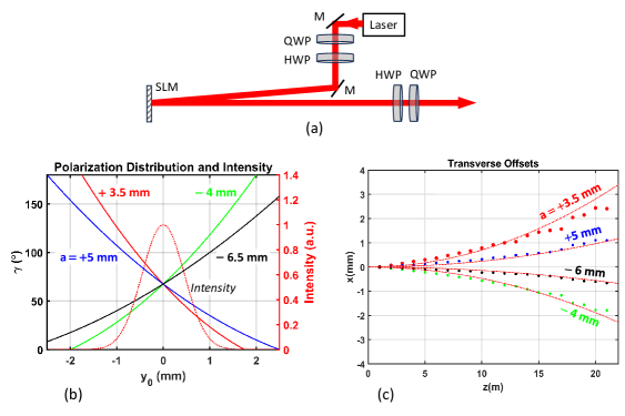
Figure 1: (a) Experimental setup (b) transverse intensity and polarization profiles and (c) the corresponding predicted and observed transverse movement of the beam centroid using the approximate theory of [4].

Figure 1 (b, c) displays the transverse intensity profile along with several transverse polarization angle distributions (obtained by varying $a$ in Eqn. (13)). The corresponding measured transverse displacements of the beam centroid $x_{c}$ are shown as a function of propagation distance $0\leq z\leq 25~{}m$. The transverse displacements were measured using the procedure described in [4]. These are compared to the approximate theory of [4] which neglects the reduction in $\vec{\Omega}$ due to diffraction to obtain, in closed form,

$$x_{c}(z)\approx\frac{\pi^{2}}{2k_{0}^{2}a^{3}}z^{2}.$$ (14)

Over the range of $z$ values shown, the approximation holds in good agreement with measurement. However, one can begin to see the predicted effects of the diffractive spreading (reduced curvature) at the longer ranges and for the smaller beam diameters which, as mentioned above, are proportional to $a$. Thus in practice there exists a trade-off between smaller $a$ (stronger initial bending, but greater reduction in curvature due to diffraction) and larger $a$ (minimal diffractive reduction in curvature, but weaker bending).

6 Model extensions

Although this paper is focused on free-space propagation, we can easily adapt the transport model to include propagation in a lossless, non-magnetic, isotropic, homogeneous medium characterized by relative permittivity $\epsilon_{1}(\vec{x},z)\neq 0$. This inclusion adds the term $k_{0}^{2}\epsilon_{1}(\vec{x},z)$ inside the brackets in (1) and, by extension, the term $\nabla_{X}\epsilon_{1}$ on the right hand side of Eqn. (3b). This term also results in the addition of the “body force"

$$\vec{s}(\vec{x},z)\equiv\rho(\vec{x},z)\nabla_{X}\epsilon_{1}(\vec{x},z)$$ (15)

to the right hand side of the conservation of momentum expression, Eqn. (5b). This holds true whether the permittivity is assumed to be a deterministic function, or is rather capturing statistical variations in the refractive index of the medium [5].

We also note that while we have considered coherent, fully polarized, monochromatic light, our model holds more generally for polychromatic, partially coherent, partially polarized light. The only difference is that one has to re-define beam intensity, transverse phase gradient, and transverse polarization angle gradient as appropriate statistical quantities. In the more general setting, these quantities were defined as averages over both time and spatial frequency in [5]. Appropriately, these quantities reduce to their coherent, monochromatic, fully polarized counterparts in those respective limits. Thus, the model (3) or (5) represents a very general model for vector beam propagation under a wide variety of conditions.

7 Summary

We have shown that paraxial beam propagation can in general be described by the model (3). The model is entirely consistent with the conservation equations found in many areas of continuum mechanics and can alternatively be written in the form (5). The model also clearly suggests a more general Poynting vector (6) which handles the spatially non-uniform polarization case, but reduces to the standard form for uniformly polarized light. The acceleration of a beam in the transverse plane is viewed appropriately as a momentum exchange where by an initial momentum, captured in the model by the polarization gradient is converted to classical transverse momentum during propagation. The physics of polarization gradient bending were alternatively described as a “symmetry breaking” in the Lagrangian density and as an observable manifestation of the vector potential found in other areas of physics.

An additional byproduct of the model is the interpretation of diffraction as a pressure. The notion that intensity will always seek to move away from highly concentrated regions to flatter regions is consistent with both intuition and observation.

We then validated the predictions of this model in experiment. The vector beams were generated using sequential polarization rotations and thus are accompanied by a geometric, Pantcharatnam-Berry phase gradient. Experimental measurements of the beam centroid as a function of propagation distance were then shown for different slopes and directions of the polarization gradient. These results match closely the associated parabolic paths predicted by an approximate closed-form solution to the model. The ultimate limits of the bending effect will be determined to a large extent by the strength of the polarization gradient that can be generated at the aperture as this dictates the available momentum that can be exchanged for transverse motion of the centroid. More generally, the model provided here gives practitioners a fundamentally new design tool for tailoring the behavior of light beams. New beam preparation approaches and testing longer propagation paths (numerically and experimentally) are the focus of ongoing investigations.

8 Acknowlegments

The authors would like to acknowledge support of the Office of Naval Research Codes 31 and 33 under grants N0001423WX01102, N0001422WX01660

Appendix A Appendix: Derivation of the transport model for vector beams

To derive the model (3) and the “conservation form” (5), we use the following approximate representation for a linearly-polarized field where the polarization angle $\gamma$ is allowed to vary with position $(\vec{x},z)$,

$$\{E_{X}(\vec{x},z),~{}E_{Y}(\vec{x},z)\} =\rho^{1/2}(\vec{x},z)e^{-i\phi(\vec{x},z)}\{\cos(\gamma(\vec{x},z)),~{}\sin(\gamma(\vec{x},z))\}$$ (16)

and substitute into Eq. (1). The result is the four mathematical statements:

$$k_{0}^{-1}\nabla_{X}\cdot\left[\rho(\vec{x},z)\nabla_{X}\gamma(\vec{x},z)\right] =0$$ (17a)

$$\partial_{z}\rho(\vec{x},z)+k_{0}^{-1}\nabla_{X}\cdot\left[\rho(\vec{x},z)\nabla_{X}\phi(\vec{x},z))\right] =0$$ (17b)

$$k_{0}\partial_{z}\phi(\vec{x},z)+\frac{1}{2}|\nabla_{X}\phi(\vec{x},z)|^{2}+\frac{1}{2}|\nabla_{X}\gamma(\vec{x},z)|^{2} =\frac{1}{2}\frac{\nabla_{X}^{2}\rho^{1/2}(\vec{x},z)}{\rho^{1/2}(\vec{x},z)}$$ (17c)

$$\frac{D\gamma(\vec{x},z)}{Dz} =0.$$ (17d)

Defining $\vec{v}(\vec{x},z)=k_{0}^{-1}\nabla_{X}\phi(\vec{x},x)$ and $\vec{\Omega}(\vec{x},z)=k_{0}^{-1}\nabla_{X}\gamma(\vec{x},z)$, (17a) can be added to (17b) to arrive at (3a, 5a). Taking the transverse gradient of both (17c) and (17d) yields, upon simplification, (3b) and (3c). Note that in doing so, use is made of the identity $\nabla_{X}\left(\vec{A}\cdot\vec{B}\right)=(\vec{A}\cdot\nabla_{X})\vec{B}+(\vec{B}\cdot\nabla_{X})\vec{A}+\vec{A}\times(\nabla_{X}\times\vec{B})+\vec{B}\times(\nabla_{X}\times\vec{A})$. Both $\vec{\Omega}(\vec{x},z)$ and $\vec{v}(\vec{x},z)$ are expressible as gradients of scalars, hence the cross-product terms vanish.

To arrive at the “conservation form” of the model, first multiply (3c) by $\rho(\vec{x},z)$ and add to the result the quantity

$$\left(\vec{v}(\vec{x},z)+\vec{\Omega}(\vec{x},z)\right)\left(\vphantom{\vec{\Omega}}\partial_{z}\rho(\vec{x},z)+\nabla_{X}\cdot\left[\vphantom{\vec{\Omega}}\rho(\vec{x},z)\vec{v}(\vec{x},z)+\rho(\vec{x},z)\vec{\Omega}(\vec{x},z)\right]\right)$$ (18)

which, by (3a), is identically zero. With this addition, and use of the the vector identity $\nabla_{X}\cdot\left(\vec{B}\otimes\vec{A}\right)=\vec{A}\left(\nabla_{X}\cdot\vec{B}\right)+\left(\vec{B}\cdot\nabla_{X}\right)\vec{A}$, Eqn. (3c) becomes

$$\partial_{z} \left(\rho(\vec{x},z)\vec{\Omega}(\vec{x},z)\right)+\nabla_{X}\cdot\left[\rho(\vec{x},z)\vec{v}(\vec{x},z)\otimes\vec{\Omega}(\vec{x},z)+\rho(\vec{x},z)\vec{\Omega}(\vec{x},z)\otimes\vec{v}(\vec{x},z)\right]=$$

$$-\vec{v}(\vec{x},z)\left(\vphantom{\vec{\Omega}}\partial_{z}\rho(\vec{x},z)+\nabla_{X}\cdot\left[\rho(\vec{x},z)\vec{v}(\vec{x},z)\right]\right)-\vec{\Omega}(\vec{x},z)\nabla_{X}\cdot\left[\rho(\vec{x},z)\vec{\Omega}(\vec{x},z)\right].$$ (19)

Now multiplying Eqn. (3b) by $\rho(\vec{x},z)$ and adding to Eqn. (19) then gives our momentum conservation equation (5b). Thus, under the new, more general definition of the Poynting vector,

$$\vec{P}(\vec{x},z) =\rho(\vec{x},z)\left(\vec{v}(\vec{x},z)+\vec{\Omega}(\vec{x},z)\right),$$ (20)

the system (5) express conservation of intensity and conservation of momentum for polarization gradient vector beams.

Appendix B Total Transverse Momentum Conservation

Equations (5a) and (5b) are local expressions of conservation in the transverse plane in the sense that they depend on $\vec{x}$. Using the Reynolds Transport Theorem (see e.g., [37], [38]) we can relate these expressions to global statements of conservation. Specifically, Eqn. (5a) can be integrated in the transverse plane to yield

$$\frac{d}{dz}\int_{X_{z}}\rho(\vec{x},z)d\vec{x} =0.$$ (21)

In other words, the total intensity is conserved on propagation, although its distribution in the transverse plane may be altered under action of the field $\vec{v}(\vec{x},z)+\vec{\Omega}(\vec{x},z)$ (via 3a).

Likewise, Eqn. (5b) expresses the conservation of transverse linear momentum. By integrating this expression in the transverse plane and again applying the Transport Theorem to the left hand side of (5b) and the well known Divergence Theorem to the right hand side of Eqn. (5b), the expression can be written

$$\frac{d}{dz}\int_{X_{z}}\vec{P}(\vec{x},z)d\vec{x}=-\int_{\partial X_{z}}{\bf P}\cdot\hat{n}~{}ds=0$$ (22)

where $ds=\sqrt{dx^{2}+dy^{2}}$ is the differential element along the closed curve $\partial_{X_{z}}$ which physically defines the transverse boundary of the beam as it propagates. Along this boundary the intensity approaches zero by definition and therefore so too does ${\bf P}$ (by Eqn. 9), hence diffraction does not change the total transverse linear momentum per unit length of propagation distance. This was also the conclusion of [39] in analyzing the analogous “quantum pressure” term found in hydrodynamic models of Schrödingers equation [40, 15].

Lastly, we note that we could have written these global, transverse conservation laws with $t$ as the independent variable by re-defining $\epsilon_{0}\rho(\vec{x},z)/c^{2}\sim[kg/m^{3}]$ (mass per unit volume) and $\epsilon_{0}\vec{P}(\vec{x},z)/c^{2}\sim[kg\cdot(m/s)\cdot m^{-3}]$ (transverse linear momentum density). This alternative representation is realized by allowing $z\rightarrow ct$ and multiplying Eqns. (5) by the free-space permittivity $\epsilon_{0}$.

Appendix C Polarization gradients and the Berry Phase

The electric field model (2) does not explicitly include the Pacharatnam-Berry (PB) phase that was acquired in creating the polarization gradient [4]. However, at the aperture ($z=0$) the geometric PB phase and polarization angle are directly related so that the subsequent evolution in the transverse gradient of the latter (Eqn. 3c) can be viewed as predicting the transverse gradient of the former.

To see this in more detail, we recall from our earlier work that the PB phase is generally a function of polarization angle, $F(\gamma(\vec{x}))$. For our particular experiment, this relationship is [4]

$$\phi_{PB}\left(\vec{x}\right) =F(\vphantom{\vec{\Omega}}\gamma(\vec{x}))=-\frac{1}{2}\left(A\cos\left(\vphantom{\vec{\Omega}}2\gamma(\vec{x})\right)+B\right)$$ (23)

that is, during our process of creating the polarization angle gradient, the beam acquires a PB phase proportional to the cosine of twice the polarization angle. Taking the transverse gradient of (23), rearranging, and multiplying by the intensity we can write

$$\rho(\vec{x},0)\vec{\Omega}(\vec{x},0) =\frac{\rho(\vec{x},0)k_{0}^{-1}\nabla_{X}F\left(\vphantom{\vec{\Omega}}\gamma(\vec{x},0)\right)}{F^{\prime}\left(\gamma(\vec{x},0)\right)}=\frac{\rho(\vec{x},0)k_{0}^{-1}\nabla_{X}\phi_{PB}\left(\vphantom{\vec{\Omega}}\vec{x}\right)}{A\sin\left(2\gamma(\vphantom{\vec{\Omega}}\vec{x},0)\right)}.$$ (24)

The polarization gradient is therefore proportional to a transverse PB phase gradient, a relationship also noted in [41], Eqn. 4. The factor in the denominator, $F^{\prime}(\gamma(\vec{x},0))\equiv dF(\gamma(\vec{x}))/d\gamma(\vec{x})$, stems from applying the chain rule in differentiating (24) and depends in general on the particular sequence of transformations that lead to the polarization gradient.

Our polarization gradient momentum could therefore also be described as a transverse momentum associated with a geometric phase gradient. Put another way, the dynamic and geometric phases give rise to corresponding, distinct momenta. Once the the beam leaves the aperture, the transverse gradients $\vec{v}(\vec{x},z),~{}\vec{\Omega}(\vec{x},z)$ evolve according to (3b) and (3c) respectively although they clearly remain coupled on propagation in such a way that the latter is eventually converted to the former causing the observed acceleration.

References

- [1] G. Milione, S. Evans, D. A. Nolan, and R. R. Alfano, “Higher order Pancharatnam-Berry phase and the angular momentum of light,” \JournalTitlePhysical Review Letters 108, 190401 (2012).
- [2] B. Zhao, V. Rodríguez-Fajardo, X.-B. Hu, R. I. Hernandez-Aranda, B. Perez-Garcia, and C. Rosales-Guzmán, “Parabolic-accelerating vector waves,” \JournalTitleNanophotonics 11, 681–688 (2022).
- [3] W.-Y. Wang, T.-Y. Cheng, Z.-X. Bai, S. Liu, and J.-Q. Lü, “Vector optical beam with controllable variation of polarization during propagation in free space: A review,” \JournalTitleApplied Sciences 11, 10664 (2021).
- [4] J. M. Nichols, D. V. Nickel, and F. Bucholtz, “Vector beam bending via a polarization gradient,” \JournalTitleOptics Express 30, 38907–38929 (2022).
- [5] J. M. Nichols, D. V. Nickel, G. K. Rohde, and F. Bucholtz, “Transport model for the propagation of partially coherent, partially polarized, polarization-gradient vector beams,” \JournalTitleJournal of the Optical Society of America - A 40, 1084–1100 (2023).
- [6] M. V. Berry, “Optical currents,” \JournalTitleJournal of Optics A: Pure and Applied Optics 11, 094001 (2009).
- [7] A. Bekshaev, K. Y. Bliokh, and M. Soskin, “Internal flows and energy circulation in light beams,” \JournalTitleJournal of Optics 13, 053001 (2011).
- [8] D. Paganin and K. A. Nugent, “Noninterferometric phase imaging with partially coherent light,” \JournalTitlePhysical Review Letters 80, 2586–2589 (1998).
- [9] K. A. Nugent and D. Paganin, “Matter-wave phase measurement: A noninterferometric approach,” \JournalTitlePhysical Review A 61, 063614 (2000).
- [10] M. Nieto-Vesperinas and X. Xu, “the complex Maxwell stress tensor theorem: The imaginary stress tensor and the reactive strength of orbital momentum. a novel scenery underlying electromagnetic optical forces,” \JournalTitleLight: Science & Applications 11, 297 (2022).
- [11] M. Lax, W. H. Louisell, and W. B. McKnight, “From Maxwell to paraxial wave optics,” \JournalTitlePhysical Review A 11, 1365–1370 (1975).
- [12] J. M. Nichols, T. H. Emerson, and G. K. Rohde, “A transport model for broadening of a linearly polarized, coherent beam due to inhomogeneities in a turbulent atmosphere,” \JournalTitleJournal of Modern Optics 66, 835–849 (2019).
- [13] M. Saeedipour and S. Schneiderbauer, “toward a universal description of multiphase turbulence phenomena based on the vorticity transport equation,” \JournalTitlePhysics of Fluids 34, 073317 (2022).
- [14] A. Davis and V. Onoochin, “The Maxwell Stress Tensor and electromagnetic momentum,” \JournalTitleProgress In Electromagnetics Research Letters 94, 151–156 (2020).
- [15] P. Mocz and S. Succi, “Numerical solution of the nonlinear Schrödinger equation using smoothed-particle hydrodynamics,” \JournalTitlePhysical Review E 91, 053304 (2015).
- [16] T. Latychevskaia, D. Schachtler, and H.-W. Fink, “Creating airy beams employing a transmissive spatial light modulator,” \JournalTitleAppl. Opt. 55, 6095–6101 (2016).
- [17] S. Pancharatnam, “Generalized theory of interference, and its applications,” \JournalTitleProceedings of the Indian Academy of Sciences-Section A 44, 247–262 (1956).
- [18] M. V. Berry, “Quantal phase factors accompanying adiabatic changes,” \JournalTitleProceedings of the Royal Society of London A 392, 45–57 (1984).
- [19] Z. Bomzon, V. Kleiner, and E. Hasman, “Pancharatnam-Berry phase in space-variant polarization manipulations with subwavelength gratings,” \JournalTitleOptics Letters 26, 1424–1426 (2001).
- [20] A. H. Dorrah, M. Tamagnone, N. A. Rubin, and F. Capasso, “Introducing Berry phase gradients along the optical path via propagation-dependent polarization transformations,” \JournalTitleNanophotonics 11, 713–725 (2022).
- [21] C. McDonnell, J. Deng, S. Sideris, G. Li, and T. Ellenbogen, “Terahertz metagrating emitters with beam steering and full linear polarization control,” \JournalTitleACS Nano Letters 22, 2603–2610 (2022).
- [22] C. P. Jisha, S. Nolte, and A. Alberucci, “Geometric phase in optics: From wavefront manipulation to waveguiding,” \JournalTitleLaser & Photonics Reviews 15, 2100003 (2021).
- [23] K. Y. Bliokh, F. J. R.-F. no, F. Nori, and A. V. Zayats, “Spin-orbit interactions of light,” \JournalTitleNature Photonics 9, 796–808 (2015).
- [24] D. Babson, S. P. Reynolds, R. Bjorkquist, and D. J. Griffiths, “Hidden momentum, field momentum, and electromagnetic impulse,” \JournalTitleAmerican Journal of Physics 77, 826–833 (2009).
- [25] D. J. Griffiths, “Resource letter em-1: Electromagnetic momentum,” \JournalTitleAmerican Journal of Physics 80, 7–18 (2012).
- [26] J. L. Jiméenez, I. Campos, and J. A. E. Roa-Neri, “The Feynman paradox and hidden momentum,” \JournalTitleEuropean Journal of Physics 43, 055202 (2022).
- [27] E. J. Konopinski, “What the electromagnetic vector potential describes,” \JournalTitleAmerican Journal of Physics 46, 499–502 (1978).
- [28] A. A. Martins and M. J. Pinheiro, “On the Electromagnetic origin of inertia and inertial mass,” \JournalTitleInternational Journal of Theoretical Physics 47, 2706–2715 (20008).
- [29] Y. Buggy, L. G. Phillips, and P. Ohberg, “On the hydrodynamics of nonlinear gauge-coupled quantum fluids,” \JournalTitleThe European Physical Journal D 74, 10.1140/epjd/e2020–100524–3 (2020).
- [30] J. D. Jackson and L. B. Okun, “Historical roots of gauge invariance,” \JournalTitleReviews of modern physics 73, 663–680 (2001).
- [31] A. Y. Bekshaev and M. S. Soskin, “Transverse energy flows in vectorial fields of paraxial beams with singularities,” \JournalTitleOptics Communicatinos 271, 332–348 (2007).
- [32] K. Y. Bliokh and Y. P. Bliokh, “Modified geometrical optics of a smoothly inhomogeneous isotropic medium: The anisotropy, Berry phase, and the optical Magnus effect,” \JournalTitlePhysical Review E 70, 026605 (2004).
- [33] K. Y. Bliokh, “Geometrodynamics of polarized light: Berry phase and spin Hall effect in a gradient-index medium,” \JournalTitleJournal of Optics A: Pure and Applied Optics 11, 094009 (2009).
- [34] A. Aiello, N. Lindlein, C. Marquardt, and G. Leuchs, “Transverse angular momentum and geometric spin Hall effect of light,” \JournalTitlePhysical Review Letters 103, 100401 (2009).
- [35] K. Y. Bliokh, “Geometrical optics of beams with vortices: Berry phase and orbital angular momentum Hall effect,” \JournalTitlePhysical Review Letters 97, 043901 (2006).
- [36] S. C. Tiwari, “Geometric phase in optics,” \JournalTitleJournal of Modern Optics 39, 1097–1105 (1992).
- [37] J. D. Achenbach, Wave propagation in elastic solids (North-Holland Pub. Co., Amsterdam, 1973).
- [38] J. E. Marsden and T. J. R. Hughes, Mathematical Foundations of Elasticity (Prentice-Hall, Englewood Cliffs, NJ, 1983).
- [39] S. K. Ghosh, “A classical view of quantum chemistry,” \JournalTitleCurrent Science 52, 769–774 (1983).
- [40] C. Nore, M. E. Brachet, and S. Fauve, “Numerical study of hydrodynamics using the nonlinear schrodinger equation,” \JournalTitlePhysica D 65, 154–162 (1993).
- [41] Y. Liu, X. Ling, X. Yi, X. Zhou, S. Chen, Y. Ke, H. Luo, and S. Wen, “Photonic spin Hall effect in dielectric metasurfaces with rotational symmeetry breaking,” \JournalTitleOptics Letters 40, 756–759 (2015).