Reinforcement Learning with Intrinsically Motivated Feedback Graph for Lost-sales Inventory Control
LIU Zifan
\AFF
Department of Electronic and Computer Engineering,
The Hong Kong University of Science and Technology,
zliuft@connect.ust.hk
\AUTHORLI Xinran
\AFF
Department of Electronic and Computer Engineering,
The Hong Kong University of Science and Technology,
xinran.li@connect.ust.hk
\AUTHORChen Shibo
\AFF
Department of Electronic and Computer Engineering,
The Hong Kong University of Science and Technology,
eeshibochen@ust.hk
\AUTHORLI Gen
\AFF
Department of Statistics,
The Chinese University of Hong Kong,
genli@cuhk.edu.hk
\AUTHORJIANG Jiashuo
\AFF
Department of Industrial Engineering and Decision Analytics,
The Hong Kong University of Science and Technology,
jsjiang@ust.hk
\AUTHORJun Zhang
\AFF
Department of Electronic and Computer Engineering,
The Hong Kong University of Science and Technology,
eejzhang@ust.hk
Reinforcement learning (RL) has proven to be well-performed and general-purpose in the inventory control (IC). However, further improvement of RL algorithms in the IC domain is impeded due to two limitations of online experience. First, online experience is expensive to acquire in real-world applications. With the low sample efficiency nature of RL algorithms, it would take extensive time to train the RL policy to convergence. Second, online experience may not reflect the true demand due to the lost sales phenomenon typical in IC, which makes the learning process more challenging. To address the above challenges, we propose a decision framework that combines reinforcement learning with feedback graph (RLFG) and intrinsically motivated exploration (IME) to boost sample efficiency. In particular, we first take advantage of the inherent properties of lost-sales IC problems and design the feedback graph (FG) specially for lost-sales IC problems to generate abundant side experiences aid RL updates. Then we conduct a rigorous theoretical analysis of how the designed FG reduces the sample complexity of RL methods. Based on the theoretical insights, we design an intrinsic reward to direct the RL agent to explore to the state-action space with more side experiences, further exploiting FG’s power. Experimental results demonstrate that our method greatly improves the sample efficiency of applying RL in IC. Our code is available at https://anonymous.4open.science/r/RLIMFG4IC-811D/
1 Introduction
Inventory control (IC) is a crucial and practical problem, serving as the basis of business efficiency for supply chain management. IC problems are challenging due to the intractability caused by the inherent complexity and the difficulty of finding optimal solutions within a reasonable timeframe. In the past few decades, researchers Zipkin (2008a), Bai et al. (2023), Xin (2021), and Chen et al. (2024) have designed a few heuristic methods based on specific model assumptions. However, such methods often face challenges due to the curse of dimensionality (Goldberg et al. 2021), where the problem size grows exponentially as the lead time increases. Here lead time refers to the duration between placing and receiving an order. Another limitation is that these model-based methods are not flexible enough to generalize to various environmental settings. These limitations call for a more adaptable approach to IC problems, for which data-driven control methods stand out as a promising alternative.
Reinforcement learning (RL) has gained significant attention as a powerful data-driven technique for solving complex sequential decision-making problems. In particular, it offers several advantages for addressing the challenges of IC problems. Firstly, RL allows for the discovery of optimal policies without relying on strong problem-specific assumptions, enabling more generalizable solutions (Nian et al. 2020). Secondly, when combined with the deep neural network, Deep RL (DRL) can handle large state and action spaces, making it suitable for problems with high-dimensional state variables (Dehaybe et al. 2024). Early works demonstrate the feasibility of RL in IC problems. Oroojlooyjadid et al. (2022) showcases the ability of a Deep Q-network (DQN) to discover near-optimal solutions for the widely recognized beer distribution game. Gijsbrechts et al. (2022) introduces the A3C algorithm into IC problems and show that it can achieve acceptable performance but not better than heuristic methods. Stranieri and Stella (2023) benchmarks various DRL methods such as A3C, PPO, and vanilla policy gradient (VPG) in IC problems. More recently, researchers tend to explore how DRL can address various scenarios within the IC problems. These scenarios include: non-stationary uncertain demand (Dehaybe et al. 2024, Park et al. 2023), multi-product (Sultana et al. 2020, Selukar et al. 2022), variable kinds of products (Meisheri et al. 2020, 2022), multi-echelon supply chains (Wu et al. 2023, Stranieri et al. 2024), one-warehouse multi-retailer (Kaynov et al. 2024), and the stochastic capacitated lot sizing problem (Van Hezewijk et al. 2023).
However, traditional RL methods are characterized by low sample efficiency, which becomes a significant barrier when implementing these techniques in real-world IC scenarios, as obtaining experiences can be both costly and time-consuming (Boute et al. 2022, De Moor et al. 2022). Furthermore, this sample inefficiency issue is enlarged in lost-sales IC problems because of censored demands (Chen et al. 2024), which refers to the phenomenon when customers’ real demands are unobservable due to insufficient inventory. For instance, if the order is placed daily, it takes over a year to generate four hundred experiences and part of them may be censored, making them too few to update the RL policy. De Moor et al. (2022) tries to alleviate this problem by incorporating heuristic knowledge, such as the base-stock policy, into DQN with reward-shaping. Although this method can improve the sample efficiency, it still relies on specific model heuristics, making it hard to generalize to different scenarios. Overall, resolving the low sample efficiency of RL without strong heuristics is crucial in solving IC (especially lost-sales IC) problems. The detailed related work is in Appendix 6.
By addressing the above-mentioned limitation, this paper proposes a novel decision framework that combines the reinforcement learning with feedback graphs (RLFG) and intrinsically motivated exploration (IME):
1) We tailor the feedback graph (FG) based the general property of lost-sales IC problems rather than strong heuristics (e.g. known demand distribution). In particular, the connectivity of FG is adjusted dynamically based on the relationship between the demand and inventory rather than being static in the environment. With FG, the sample efficiency in the training process is significantly improved by allowing the agent to acquire not only online experiences but also side experiences from FG.
2) We conduct a theoretical analysis of how FG reduces the sample complexity with Q-learning as an example. It demonstrates that FG decreases the sample complexity by improving the update probabilities across all state-action pairs.
3) Inspired by these theoretical insights, we design a novel intrinsic reward that guides the RL algorithm to explore towards the state-action space where more side experiences can be obtained thereby further boosting sample efficiency.
4) We evaluate our method on the standard discrete lost-sales inventory control environment. Our empirical results demonstrate the superior sample efficiency improvement by FG and the intrinsic reward separately, underlining the effectiveness of our design.
2 Background and Problem Formulation
2.1 Reinforcement Learning with Feedback Graph
RLFG is proposed by Dann et al. (2020) to reduce the sample complexity of RL. In typical RL scenarios, an agent can only get one experience each time as feedback that can be used to update the policy. However, when some prior knowledge about the environments is available, it becomes possible to observe additional experiences involving other states and actions. RLFG aims to explore how RL algorithms can benefit from these side experiences by constructing a feedback graph (FG). Here “side experiences” bears the same meaning as “side observations” in Dann et al. (2020), and we use the term “side experiences” to avoid confusion with “observations” in partially observed MDPs. FG is a directed graph , where is the vertex set and is the edge set , formalized by the side information indicating that if the agent visits , it can also observe other vertices . The total experiences observed by the agent at from is
| (1) |
2.2 Lost Sales Inventory Control Problem
| Symbol | Representation | Symbol | Representation |
|---|---|---|---|
| Order lead time | Order at time | ||
| Time index | Maximum order | ||
| Real demand in period | Unit cost of procurement | ||
| Demand observed in period | Unit cost of holding inventory | ||
| Maximum demand | Unit cost penalty of lost sales | ||
| State: | Discount factor | ||
| Inventory at time , | Maximum inventory at time , | ||
| after the order due at arrives | after the order due at arrives |
We formulate a standard, single-item, discrete-time, and lost-sales IC problem following Zipkin (2008a), Gijsbrechts et al. (2022) and Xin (2021) with environment variables in Table 1. The “lost-sales” means that customers leave if there is not enough inventory without any way to record the excess demand. The lost-sales IC problem considers three kinds of costs in each time step , which are the cost of procurement , the cost of holding inventory , and the cost penalty of lost sales . The cost terms are specified below, where .
| (2) |
In this problem, the real demand is unobservable when it exceeds the current inventory. Thus we define the real demand as a random variable and the observed demand , which may be censored by and , given as
| (3) |
Here, the term “censored” indicates the otherwise case in Equation 3, when we can only observe all inventory is sold but do not know the value of . The objective is to minimize the total cost over the time horizon under the uncertainty on the demand side, which is
| (4) |
2.3 MDP Formulation
To better understand the lost-sales IC problem from the perspective of RL, we formulate it into an infinite-horizon MDP with discounted rewards (Li et al. 2020), represented by . The MDP consists of the state space , action space , transition function , reward function , and discount factor . The detailed composition of MDP is shown as follows:
State: The state includes the inventory at time after receiving the orders and all upcoming orders due to lead time. We define it as .
Action: The action is the amount to be ordered for future sales, given as , where is the maximum amount that can be ordered for this item.
Reward: Since the goal is to minimize the cumulative discounted cost, the reward at each time step is defined as the opposite number of costs, which is .
Transition Function: The transition function is defined as . The inventory transition is defined as due to the lead time. As has been received, in will replace in for .
3 Method
3.1 IC Decision Framework with RLFG and IME
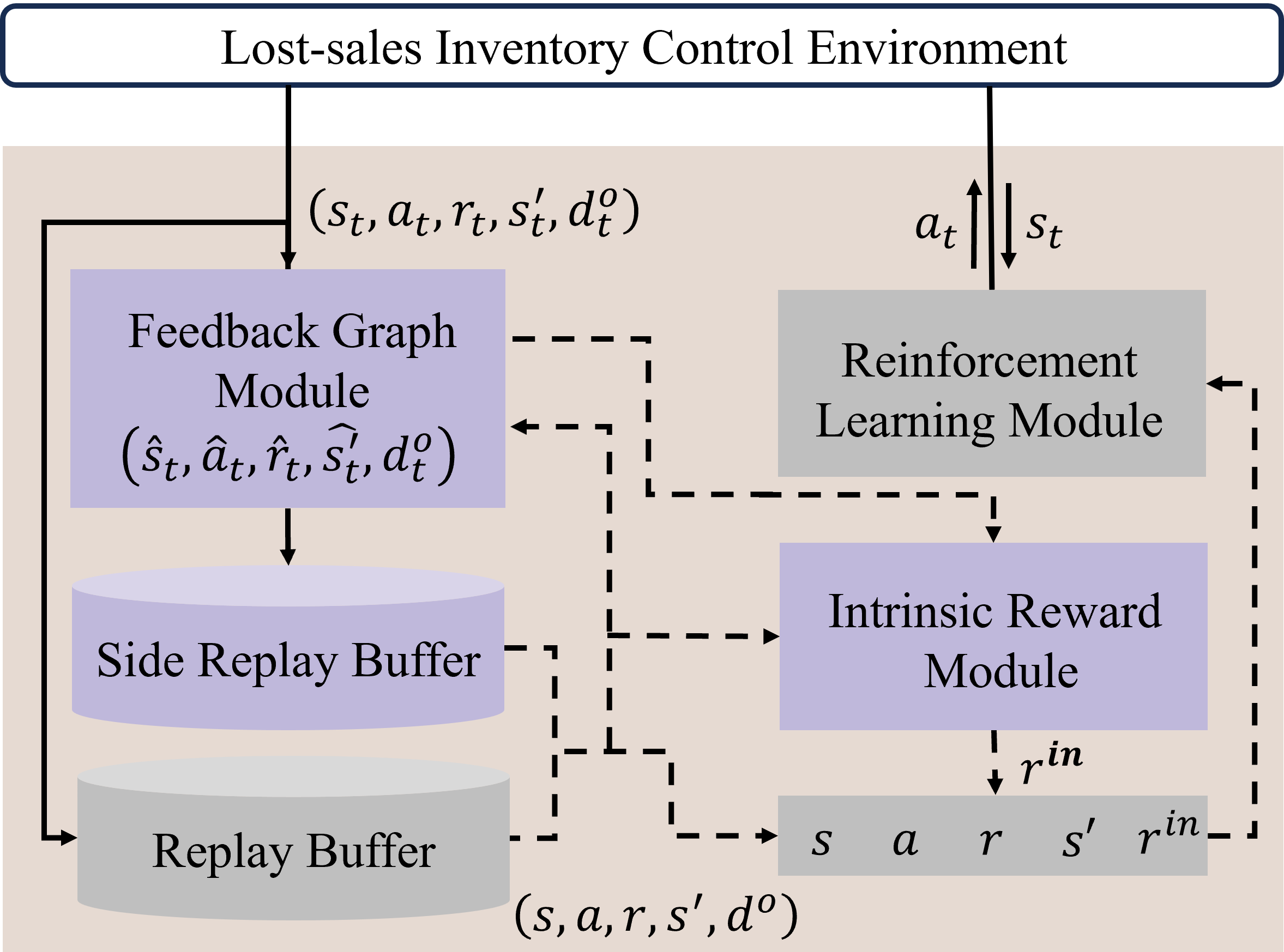
The proposed decision framework for IC problems aims to enhance the sample efficiency of off-policy RL algorithms by integrating RLFG and IME together. This framework relies on two key assumptions. First, the real demand is unknown and the observed demand may be censored. Second, the experiences generated in real-world operations are limited due to the cost involved in collecting online data. As illustrated in Figure 1, the FG module generates side experiences to improve the sample efficiency and the intrinsic reward module aids the exploration to further exploit the power of the FG module. Here, the RL module can be any off-policy RL algorithm, such as DQN, DDPG, Rainbow, or TD3. Note that experiences from both reply buffers are sampled with no differences in the model-updating step. Then a new set of side experiences are generated based on the sampled experiences. These new side experiences are just used to calculate intrinsic rewards of the sampled experiences. Here we provide Rainbow-FG as an example in Algorithm 1.
3.2 Feedback Graph in Inventory Control
Motivated by the reduction in sample complexity by FG (Dann et al. 2020), we incorporate FG into the IC problem. FG is naturally suitable for the IC problem since the IC problem is a structured MDP with most environmental transition components determined and predictable depending on the demand. Furthermore, the demand is usually independent of the state-action space. If we can observe the demand, the experiences of other state-action pairs can also be obtained through leveraging the underlying properties of such structured MDPs. Thus the main challenge is how to construct FG considering the lost-sales property, whose demand is potentially censored. To solve this problem, we propose to construct FG dynamically based on the observed demand. If the observed demand is real, FG generates side experiences of all other state-action pairs. Even if the observed demand is censored, FG can generate side experiences of the state-action pairs whose inventory is less than the observed demand.
Algorithm 2 shows the details of the FG module. When is uncensored, FG is a complete graph and all state-action pairs can be used to generate side experiences based on . When is censored, it becomes more complex. For the state-action pairs having larger inventory numbers than that in , is not a correct demand for them and unfortunately is unknown. Still using will generate wrong side experiences. We can only use the state-action pairs having smaller inventory numbers than that in to generate side experiences, which means that FG is a partially connected graph. Note that FG is still dynamically constructed based on under the censored case since different generates different numbers of side experiences.
3.3 Theoretical Analysis
We conduct a quantitative analysis of how the sample complexity is reduced with the FG in the lost-sales IC environment. The qualitative analysis based on the property of RLFG is in Appendix 7. Here we provide an analysis based on Q-learning for simplicity. The detailed proof is in Appendix 8
Without loss of generality, we restrict some definitions in section 2.3 and define some new concepts. We consider the reward function . The demand can obey any independent discrete distribution and . We define as the stationary behavior policy and as the stationary distribution of the Markov chain under and , which is the same as the update probability in typical RL. In RLFG, the stationary distribution does not change but the update probability becomes because of the side experiences.
Scenario 1: Consider a graph with all state-action pairs as the nodes and there is no edge between the nodes. It can be regarded as , where and consists of nodes without any edge.
Lemma 1: The sample complexity of the asynchronous Q-learning under scenario 1 is analyzed in Li et al. (2020), which is , where and is the mixing time of the chain.
Lemma 1 indicates that the sample complexity of Q-learning without FG is determined by . We will show how Q-learning with FG improves to reduce the sample complexity.
Scenario 2: Consider a graph with all state-action pairs as the nodes. Assume for nodes satisfying , once one node is sampled, all of these nodes can be sampled and updated simultaneously. For nodes with , only nodes with can be sampled and updated simultaneously. Thus can be regarded as .
Theorem 1: The update probability for Q-learning with FG under scenario 2 is:
| (5) |
Conclusion: We can obtain the relationship between and in Equation (6). It shows that FG not only improves but also improves that of all the state-action pairs.
| (6) |
3.4 Intrinsically Motivated Exploration
To further utilize the benefits of FG, we design an intrinsic reward by incorporating the information of the side experiences into the curiosity-driven exploration. In particular, for a state-action pair, the number and the average uncertainty of the side experiences generated by this state-action pair are incorporated into the intrinsic reward. With this intrinsic reward, the agent is directed towards the state-action space where more side experiences can be generated.
This idea is inspired by the theoretical analysis based on Equation 5. The uncensored term indicates how much the uncensored case contributes to improving the probability of being updated. This term contributes to all state-action pairs so improving this term can improve the probability of being updated for all state-action pairs. The censored term indicates how much benefit the current state-action pair can obtain from the censored cases. For the censored case, the sample complexity can be further reduced by visiting the state-action pairs with larger inventory. To satisfy both conditions, designing a behavior policy manually is difficult and not general enough. Thus we design an intrinsic reward, written in Equation 7 because both conditions lead to generating more side observations.
| (7) |
Algorithm 3 shows the details of the intrinsic reward module. We utilize the M-head DQN (Nikolov et al. 2018) with each head trained by different mini-batch of experiences to get the prediction error as curiosity rewards. The final intrinsic reward, denoted in Equation 7, consists of the curiosity reward of the experience itself () and the averaged curiosity reward of all corresponding side experiences () generated by this experience. The averaged value preserves the advantage of scale invariance but loses the quantity information compared with the sum value. To balance these two aspects, we multiply the averaged value with to incorporate more quantity information into the intrinsic reward. In the censored condition, where , a larger increases the intrinsic reward, which means more side experiences. In the uncensored condition, is larger than , which means that the intrinsic reward is more likely to be larger than that in the censored condition.
4 Experiment
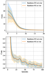
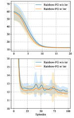
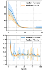
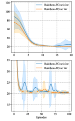
To verify the performance and sample efficiency of our decision framework, we utilize the example algorithm in Algorithm 1 and test it based on the standard lost-sales IC environment. All experiments are averaged with 20 random seeds with shaded areas representing the standard deviation.
4.1 Setup
4.1.1 Baseline
Heuristic Methods: We compare our method with widely recognized and well-performed heuristic methods. All parameters used in these methods are searched in detail and the best results are selected.
-
•
Constant Order: The order is always a constant (), where is a parameter.
-
•
Myopic 1-period (Morton 1971): Assume the distribution of is known. This method aims to minimize the expected cost at . The order is , .
-
•
Myopic 2-period (Zipkin 2008a): Since Myopic 1-period only considers the expected cost for one time step, it can be improved by considering 2-time steps.
-
•
Base-Stock method (Zipkin 2008a): The Base-Stock method aims to keep the inventory level constant, including upcoming orders. The order is , where is a parameter.
-
•
Capped Base-Stock method (Xin 2021): It combines Base-Stock and Constant Order method. The order is , where and are parameters.
-
•
Bracket method (Bai et al. 2023): A variant of the Constant Order method. The order is , where and are parameters.
Deep Reinforcement Learning Methods: We choose to compare Rainbow-FG with the A3C method in Gijsbrechts et al. (2022), which is an on-policy RL method; Rainbow, which is the basis of Rainbow-FG; Rainbow-FG(H), which utilizes the heuristic knowledge to continue finetuning Rainbow-FG. Rainbow-FG(H) can be regarded as the upper bound of Rainbow-FG. Since A3C is on-policy, it is not applicable to compare sample efficiency with off-policy Rainbow-FG. Thus A3C is only used to compare the optimal results.
| Parameter | ||||||||
|---|---|---|---|---|---|---|---|---|
| Value |
4.1.2 Environments
We test our method and baselines across different settings of the standard discrete lost-sales IC environment with demand obeying Poisson distribution, where indicates the mean value. The parameters of the environment setting are shown in Table 2 and the hyperparameters of our method are in Appendix 9. As for parameters in Table 2, we follow the common recognized settings according to Zipkin (2008a), Xin (2021), and Gijsbrechts et al. (2022). In the following sections, default parameters are used unless stated otherwise. The hyperparameter analysis is demonstrated in Appendix 12.
| Method | p=4 | p=9 | ||||
| L=2 | L=3 | L=4 | L=2 | L=3 | L=4 | |
| Optimal | 4.40 | 4.60 | 4.73 | 6.09 | 6.53 | 6.84 |
| Constant Order | 5.27 | 5.27 | 5.27 | 10.27 | 10.27 | 10.27 |
| 19.8% | 14.6% | 11.4% | 68.6% | 57.3% | 50.1% | |
| Bracket | 5.00 | 5.01 | 5.02 | 8.02 | 8.02 | 8.03 |
| 13.6% | 8.9% | 6.1% | 31.7% | 22.8% | 17.3% | |
| Myopic 1-period | 4.56 | 4.84 | 5.06 | 6.22 | 6.80 | 7.20 |
| 3.7% | 5.3% | 7.1% | 2.1% | 4.1% | 5.3% | |
| Myopic 2-period | 4.41 | 4.64 | 4.82 | 6.10 | 6.57 | 6.92 |
| 0.2% | 0.8% | 1.9% | 0.2% | 0.6% | 1.2% | |
| Base-Stock | 4.64 | 4.98 | 5.20 | 6.32 | 6.86 | 7.27 |
| 5.5% | 8.2% | 9.9% | 3.7% | 5.1% | 6.4% | |
| Capped Base-Stock | 4.41 | 4.63 | 4.80 | 6.12 | 6.62 | 6.91 |
| 0.2% | 0.7% | 1.5% | 0.5% | 1.4% | 1.0% | |
| A3C | 4.54 | 4.74 | 5.05 | 6.38 | 6.73 | 7.07 |
| 3.2% | 3.0% | 6.7% | 4.8% | 3.1% | 3.4% | |
| Rainbow | 4.52 | 4.72 | 4.91 | 6.28 | 6.72 | 7.09 |
| 2.7% | 2.6% | 3.8% | 3.1% | 2.9% | 3.7% | |
| Rainbow-FG (our) | 4.48 | 4.67 | 4.87 | 6.22 | 6.73 | 6.99 |
| 1.8% | 1.5% | 2.9% | 2.1% | 3.1% | 2.2% | |
| Rainbow-FG (H) (our) | 4.404 | 4.61 | 4.775 | 6.12 | 6.60 | 6.92 |
| 0.1% | 0.2% | 0.9% | 0.5% | 1.1% | 1.2% | |
4.2 Optimal Results Comparison
Table 3 presents the average results and optimality gap compared to the optimal results. Without strong heuristics, Rainbow demonstrates similar performance to the A3C method in Gijsbrechts et al. (2022), whereas Rainbow-FG achieves superior results. This notable improvement can be attributed to Rainbow-FG’s ability to leverage a broader range of side experiences from the feedback graph, enabling it to converge towards better solutions compared with Rainbow.
When contrasting Rainbow-FG with the heuristic methods, Rainbow-FG still falls short of surpassing the top-performing heuristic methods, such as Myopic 2-period and Capped Base-Stock. However, Myopic 2-period method assumes the distribution of the demand is known, which is a strong assumption, and the Capped Base-Stock method needs extensive parameter searches to attain this optimal result. These parameters vary across different scenarios without patterns. Conversely, Rainbow-FG consistently achieves close performance and possesses adaptability to diverse settings without these strong heuristics. Furthermore, after incorporating the heuristic knowledge, Rainbow-FG(H) attains equivalent or even superior performance compared to the best heuristic methods, particularly in certain settings. This result indicates that Rainbow-FG has the potential to perform better than heuristic methods.
4.3 Sample Efficiency Comparison for FG
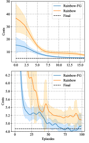
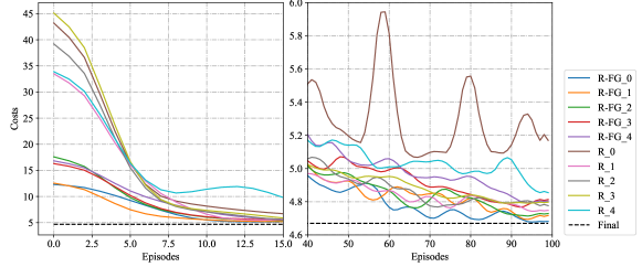
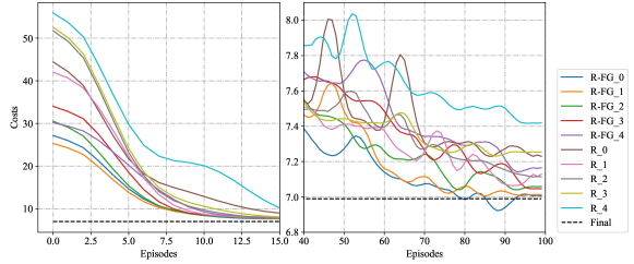
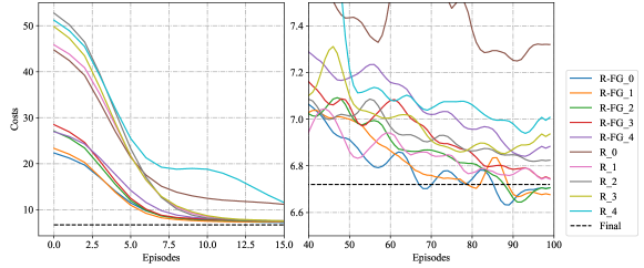
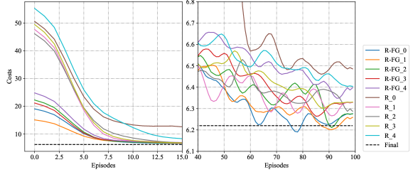
Figure 2 illustrates the learning process of Rainbow and Rainbow-FG with different exploration parameters. The utilization of FG significantly enhances the sample efficiency. During the initial stage, Rainbow-FG with all consistently outperforms Rainbow. Towards the end, Rainbow-FG with converges to the final result first and subsequently trails Rainbow-FG with . Conversely, Rainbow fails to converge to the final result throughout the entire 100 episodes. Furthermore, FG contributes to improving the stability of the learning process. Notably, the learning process of Rainbow-FG exhibits lower standard deviation and more stable learning curves. Under low exploration conditions (), Rainbow-FG demonstrates significantly faster learning compared to Rainbow. This outcome signifies the benefits of FG when exploration is not favorable. Experiments on more settings are shown in Appendix 11.
4.4 Sample Efficiency Comparison for Intrinsic Reward
This section investigates the effect of intrinsic reward designed for the IC problem. Figure 3 illustrates the learning process of Rainbow-FG with and without the intrinsic reward, referred to as Rainbow-FG w/ inr and Rainbow-FG w/o inr, respectively. The results demonstrate that the designed intrinsic reward significantly improves sample efficiency during the initial stages of training in the environment with , and . However, as the learning process reaches the Constant Order level, the intrinsic reward does not exhibit a substantial impact. We attribute it to the simplicity of the environment, which weakens the effect of the intrinsic reward. To further evaluate its effectiveness, we conduct experiments in more complex settings with , and varying values of (5, 10, 15). In these environments, we observe a clear effect of the intrinsic reward during the whole training process. Moreover, Rainbow-FG w/ inr demonstrates a more stable training process compared to Rainbow-FG w/o inr, achieving slightly lower cost.
5 Conclusion
dresses the challenge of sample inefficiency for RL methods in lost-sales IC problems. We design a novel decision framework integrating RLFG and IME to boost the sample efficiency of RL methods. We first specially tailored FG only based on the general property of lost-sales IC problems rather than strong heuristics to generate side experiences to aid RL update. We then conduct a theoretical analysis to demonstrate our method’s effectiveness with Q-learning as an example. The analysis shows that FG decreases the sample complexity by improving the update probabilities for all state-action pairs. Additionally, we design an intrinsic reward to fully utilize FG for lost-sales IC problems based on the analysis result. Experimental results show that our approach greatly enhances RL’s sampling efficiency in IC problems, which is consistent with the theoretical analysis. As for the limitation, we only analyze the magnitude relationship between and ; a detailed multiplicative relationship still needs to be proved.
References
- Alon et al. [2015] N. Alon, N. Cesa-Bianchi, O. Dekel, and T. Koren. Online learning with feedback graphs: Beyond bandits. In Conference on Learning Theory, pages 23–35. PMLR, 2015.
- Arrow et al. [1958] K. J. Arrow, S. Karlin, H. E. Scarf, et al. Studies in the mathematical theory of inventory and production. 1958.
- Bai et al. [2023] X. Bai, X. Chen, M. Li, and A. Stolyar. Asymptotic optimality of open-loop policies in lost-sales inventory models with stochastic lead times. Available at SSRN 4362329, 2023.
- Bijvank and Johansen [2012] M. Bijvank and S. G. Johansen. Periodic review lost-sales inventory models with compound poisson demand and constant lead times of any length. European Journal of Operational Research, 220(1):106–114, 2012.
- Bijvank and Vis [2011] M. Bijvank and I. F. Vis. Lost-sales inventory theory: A review. European Journal of Operational Research, 215(1):1–13, 2011.
- Bijvank et al. [2023] M. Bijvank, W. T. Huh, and G. Janakiraman. Lost-sales inventory systems. In Research Handbook on Inventory ManagemenT, pages 2–26. Edward Elgar Publishing, 2023.
- Boute et al. [2022] R. N. Boute, J. Gijsbrechts, W. Van Jaarsveld, and N. Vanvuchelen. Deep reinforcement learning for inventory control: A roadmap. European Journal of Operational Research, 298(2):401–412, 2022.
- Chen et al. [2024] B. Chen, J. Jiang, J. Zhang, and Z. Zhou. Learning to order for inventory systems with lost sales and uncertain supplies. Management Science, 2024.
- Cuartas and Aguilar [2023] C. Cuartas and J. Aguilar. Hybrid algorithm based on reinforcement learning for smart inventory management. Journal of intelligent manufacturing, 34(1):123–149, 2023.
- Dann et al. [2020] C. Dann, Y. Mansour, M. Mohri, A. Sekhari, and K. Sridharan. Reinforcement learning with feedback graphs. Advances in Neural Information Processing Systems, 33:16868–16878, 2020.
- De Moor et al. [2022] B. J. De Moor, J. Gijsbrechts, and R. N. Boute. Reward shaping to improve the performance of deep reinforcement learning in perishable inventory management. European Journal of Operational Research, 301(2):535–545, 2022.
- Dehaybe et al. [2024] H. Dehaybe, D. Catanzaro, and P. Chevalier. Deep reinforcement learning for inventory optimization with non-stationary uncertain demand. European Journal of Operational Research, 314(2):433–445, 2024.
- Gijsbrechts et al. [2022] J. Gijsbrechts, R. N. Boute, J. A. Van Mieghem, and D. J. Zhang. Can deep reinforcement learning improve inventory management? performance on lost sales, dual-sourcing, and multi-echelon problems. Manufacturing & Service Operations Management, 24(3):1349–1368, 2022.
- Goldberg et al. [2016] D. A. Goldberg, D. A. Katz-Rogozhnikov, Y. Lu, M. Sharma, and M. S. Squillante. Asymptotic optimality of constant-order policies for lost sales inventory models with large lead times. Mathematics of Operations Research, 41(3):898–913, 2016.
- Goldberg et al. [2021] D. A. Goldberg, M. I. Reiman, and Q. Wang. A survey of recent progress in the asymptotic analysis of inventory systems. Production and Operations Management, 30(6):1718–1750, 2021.
- Han et al. [2023] J. Han, M. Hu, and G. Shen. Deep neural newsvendor. arXiv preprint arXiv:2309.13830, 2023.
- Hao et al. [2022] B. Hao, T. Lattimore, and C. Qin. Contextual information-directed sampling. In International Conference on Machine Learning, pages 8446–8464. PMLR, 2022.
- Harsha et al. [2021] P. Harsha, A. Jagmohan, J. Kalagnanam, B. Quanz, and D. Singhvi. Math programming based reinforcement learning for multi-echelon inventory management. Available at SSRN 3901070, 2021.
- Janakiraman and Roundy [2004] G. Janakiraman and R. O. Roundy. Lost-sales problems with stochastic lead times: Convexity results for base-stock policies. Operations Research, 52(5):795–803, 2004.
- Jiang and Ye [2024] J. Jiang and Y. Ye. Achieving sample complexity for constrained markov decision process. arXiv preprint arXiv:2402.16324, 2024.
- Karlin [1958] S. Karlin. Inventory models of the arrow-harris-marschak type with time lag. Studies in the mathematical theory of inventory and production, 1958.
- Kaynov et al. [2024] I. Kaynov, M. van Knippenberg, V. Menkovski, A. van Breemen, and W. van Jaarsveld. Deep reinforcement learning for one-warehouse multi-retailer inventory management. International Journal of Production Economics, 267:109088, 2024.
- Li et al. [2020] G. Li, Y. Wei, Y. Chi, Y. Gu, and Y. Chen. Sample complexity of asynchronous q-learning: Sharper analysis and variance reduction. Advances in neural information processing systems, 33:7031–7043, 2020.
- Li et al. [2024] G. Li, C. Cai, Y. Chen, Y. Wei, and Y. Chi. Is q-learning minimax optimal? a tight sample complexity analysis. Operations Research, 72(1):222–236, 2024.
- Liu et al. [2018] F. Liu, S. Buccapatnam, and N. Shroff. Information directed sampling for stochastic bandits with graph feedback. In Proceedings of the AAAI Conference on Artificial Intelligence, volume 32, 2018.
- Mannor and Shamir [2011] S. Mannor and O. Shamir. From bandits to experts: On the value of side-observations. Advances in Neural Information Processing Systems, 24, 2011.
- Marinov et al. [2022] T. V. Marinov, M. Mohri, and J. Zimmert. Stochastic online learning with feedback graphs: Finite-time and asymptotic optimality. Advances in Neural Information Processing Systems, 35:24947–24959, 2022.
- Meisheri et al. [2020] H. Meisheri, V. Baniwal, N. N. Sultana, H. Khadilkar, and B. Ravindran. Using reinforcement learning for a large variable-dimensional inventory management problem. In Adaptive learning agents workshop at AAMAS, pages 1–9, 2020.
- Meisheri et al. [2022] H. Meisheri, N. N. Sultana, M. Baranwal, V. Baniwal, S. Nath, S. Verma, B. Ravindran, and H. Khadilkar. Scalable multi-product inventory control with lead time constraints using reinforcement learning. Neural Computing and Applications, 34(3):1735–1757, 2022.
- Morton [1969] T. E. Morton. Bounds on the solution of the lagged optimal inventory equation with no demand backlogging and proportional costs. SIAM review, 11(4):572–596, 1969.
- Morton [1971] T. E. Morton. The near-myopic nature of the lagged-proportional-cost inventory problem with lost sales. Operations Research, 19(7):1708–1716, 1971.
- Nian et al. [2020] R. Nian, J. Liu, and B. Huang. A review on reinforcement learning: Introduction and applications in industrial process control. Computers & Chemical Engineering, 139:106886, 2020.
- Nikolov et al. [2018] N. Nikolov, J. Kirschner, F. Berkenkamp, and A. Krause. Information-directed exploration for deep reinforcement learning. arXiv preprint arXiv:1812.07544, 2018.
- Oroojlooyjadid et al. [2022] A. Oroojlooyjadid, M. Nazari, L. V. Snyder, and M. Takáč. A deep q-network for the beer game: Deep reinforcement learning for inventory optimization. Manufacturing & Service Operations Management, 24(1):285–304, 2022.
- Park et al. [2023] H. Park, D. G. Choi, and D. Min. Adaptive inventory replenishment using structured reinforcement learning by exploiting a policy structure. International Journal of Production Economics, 266:109029, 2023.
- Reiman [2004] M. I. Reiman. A new and simple policy for the continuous review lost sales inventory model. Unpublished manuscript, 2004.
- Selukar et al. [2022] M. Selukar, P. Jain, and T. Kumar. Inventory control of multiple perishable goods using deep reinforcement learning for sustainable environment. Sustainable Energy Technologies and Assessments, 52:102038, 2022.
- Stranieri and Stella [2023] F. Stranieri and F. Stella. Comparing deep reinforcement learning algorithms in two-echelon supply chains, 2023.
- Stranieri et al. [2024] F. Stranieri, E. Fadda, and F. Stella. Combining deep reinforcement learning and multi-stage stochastic programming to address the supply chain inventory management problem. International Journal of Production Economics, 268:109099, 2024.
- Sultana et al. [2020] N. N. Sultana, H. Meisheri, V. Baniwal, S. Nath, B. Ravindran, and H. Khadilkar. Reinforcement learning for multi-product multi-node inventory management in supply chains. arXiv preprint arXiv:2006.04037, 2020.
- Tossou et al. [2017] A. Tossou, C. Dimitrakakis, and D. Dubhashi. Thompson sampling for stochastic bandits with graph feedback. In Proceedings of the AAAI Conference on Artificial Intelligence, volume 31, 2017.
- Van Hezewijk et al. [2023] L. Van Hezewijk, N. Dellaert, T. Van Woensel, and N. Gademann. Using the proximal policy optimisation algorithm for solving the stochastic capacitated lot sizing problem. International Journal of Production Research, 61(6):1955–1978, 2023.
- Wu et al. [2023] G. Wu, M. Á. de Carvalho Servia, and M. Mowbray. Distributional reinforcement learning for inventory management in multi-echelon supply chains. Digital Chemical Engineering, 6:100073, 2023.
- Xie et al. [2024] Y. Xie, W. Ma, and L. Xin. Vc theory for inventory policies. arXiv preprint arXiv:2404.11509, 2024.
- Xin [2021] L. Xin. Understanding the performance of capped base-stock policies in lost-sales inventory models. Operations Research, 69(1):61–70, 2021.
- Zipkin [2008a] P. Zipkin. Old and new methods for lost-sales inventory systems. Operations research, 56(5):1256–1263, 2008a.
- Zipkin [2008b] P. Zipkin. On the structure of lost-sales inventory models. Operations research, 56(4):937–944, 2008b.
6 Related Work
6.1 Inventory Control Problem
The inventory control (IC) problem involves determining the optimal quantity of inventory to order to minimize costs while maintaining sufficient stock levels to meet customer demand. Based on different assumptions about the behavior of the customer, the IC problem can be divided into backlogging IC and lost-sales IC problems [Chen et al., 2024]. The backlogging IC problem assumes that when the demand cannot be met due to insufficient inventory, the request of customers is accepted but delayed until inventory is replenished. Arrow et al. [1958] has proven that the base-stock policy, which aims to keep the sum of inventory level and upcoming orders constant, is optimal for single-source backlogging IC with constant lead time. Compared with backlogging IC, the lost-sales IC problem is more complex and relevant [Bijvank and Vis, 2011]. the lost-sale IC problem assumes that when demand cannot be met due to insufficient inventory, the customer’s request is lost and the exceeding request is unobservable, such as e-commerce. The base-stock policy can only be optimal when the cost of the lost-sales penalty is high. This motivates researchers to find better methods for the lost-sales IC problem.
6.2 Heuristic Methods in Lost-sales Inventory Control
The lost-sales IC problem is first simply studied by Karlin [1958], which assumes the lead time to place orders is one. Karlin [1958] proves that base-stock policy is not optimal because the inventory availability in future periods cannot be characterized by the inventory level and order quantity. Morton [1969] extends the former analysis to any positive and integral-value lead time and provides the upper and lower bounds of the optimal policy. Furthermore, Zipkin [2008b] generalizes to any lead times from the aspect of L-natural-convexity, and Janakiraman and Roundy [2004] studies the case when lead time is stochastic. The base-stock policy is sensitive to the demand due to its design. The opposite one is the Constant Order policy, whose decision has no relationship with the demand [Bijvank et al., 2023]. As the lead time goes to infinity, Goldberg et al. [2016] proves that the constant-order policy can be asymptotically optimal and Reiman [2004] proves that the constant-order policy can be better than the base-stock policy. The contrary properties of these two methods motivate a better idea that combines both advantages [Bijvank and Johansen, 2012]. Xin [2021] improves this idea to a new method named capped base-stock policy.
The above-introduced methods need to search for the best parameter for specific settings to perform well. Besides them, there is another serious of heuristic method, also called approximate dynamic programming (APD). These methods assume known demand distribution rather than parameter searching. Morton [1971] proposes the Myopic method, which aims to minimize the expected cost when the placed order arrives. This method can be extended to the Myopic-T method, which considers the expected cost for time steps.
6.3 Reinforcement Learning Method in Inventory Control
The heuristic method needs either a parameter search or an assumption about the demand distribution, which are not general enough. This motivates the studies about applying reinforcement learning (RL) to lost-sales IC problems. RL has gained significant attention as a powerful data-driven technique for solving complex sequential decision-making problems [Han et al., 2023, Jiang and Ye, 2024, Xie et al., 2024]. RL offers several advantages for addressing the challenges of IC problems. Firstly, RL allows for the discovery of optimal policies without relying on strong problem-specific assumptions, enabling more generalizable solutions [Nian et al., 2020]. Secondly, combined with the deep neural network, Deep RL (DRL) can handle large state and action spaces, making it suitable for problems with high-dimensional variables [Dehaybe et al., 2024]. Initially, the work mainly focuses on verifying the feasibility of RL in IC problems. Oroojlooyjadid et al. [2022] showcases the ability of a Deep Q-Network (DQN) to discover solutions that are close to optimal for the widely recognized beer distribution game. Gijsbrechts et al. [2022] introduces the A3C algorithm into IC problems and show that A3C can achieve acceptable performance but not better heuristic methods. Stranieri and Stella [2023] benchmarks various DRL methods such as A3C, PPO, and vanilla policy gradient (VPG) in IC problems. Recently, researchers tend to study how DRL can solve different situations of IC problems such as, non-stationary uncertain demand [Dehaybe et al., 2024, Park et al., 2023], multi-product [Sultana et al., 2020, Selukar et al., 2022], variable kinds of products [Meisheri et al., 2020, 2022], multi-echelon supply chains [Wu et al., 2023, Stranieri et al., 2024], one-warehouse multi-retailer [Kaynov et al., 2024], stochastic capacitated lot sizing problem [Van Hezewijk et al., 2023].
However, Two fundamental issues have not been resolved. First, the final performance of DRL is not optimal, sometimes even worse than heuristic methods. To address this problem, some papers [Cuartas and Aguilar, 2023, Stranieri et al., 2024, Harsha et al., 2021] explore the potential to combine RL algorithms with existing other methods rather than directly applying RL to IC problems. The other problem is the low sample efficiency nature of existing RL methods, which restricts further application to real-world IC problems [Boute et al., 2022, De Moor et al., 2022], especially when obtaining experiences is expensive or time-consuming. Besides, this sample inefficiency problem is enlarged in lost-sales IC because of censored demands [Chen et al., 2024], which refers to the phenomenon when the customer’s real demand is unobservable due to insufficient inventory. Typically, if the order is placed daily, generating four hundred experiences needs over a year and part of them may be censored making them too hard to update RL policy. De Moor et al. [2022] tries to alleviate this problem by incorporating heuristic knowledge, such as base-stock policy, into DQN with reward-shaping. Although this method can improve the sample efficiency, it still relies on specific model heuristics, making it hard to generalize to different scenarios. Overall, Resolving the low sample efficiency of RL without strong heuristics is crucial in solving IC (especially lost-sales IC) problems.
6.4 Feedback Graph and its Application
Mannor and Shamir [2011] first proposes the feedback graph (FG) idea as a method to reduce the regret bound of the bandit problem when side observations can be obtained assuming the decision maker can also know the situations when other actions are taken besides the chosen action. Alon et al. [2015] extends the analysis of FG on bandit problems beyond the learning problems. Tossou et al. [2017] gives the first analysis of Thompson sampling for bandits with FG based on information theory. Building upon these foundations, Dann et al. [2020] combines FG with RL and shows how FG can reduce the regret bound and sample complexity of model-based RL algorithms. However, most existing work, such as Liu et al. [2018], Hao et al. [2022], and Marinov et al. [2022], mainly focus on the analysis of FG in some bandits problems. Seldom work tries to apply FG to real-world problems since side observations and the structure of FG are hard to define in applications.
7 Analysis based on the Property of Graph
Based on the feedback graph , Dann et al. [2020] defines three concepts to measure the sample complexity. , , and measure the minimum vertices to be sampled to observe the whole . We will talk about , , and for the IC environment in section 3.2.
Mas-number(): The maximum size of forming an acyclic subgraph of is the mas-number.
Independence number(): The size of the largest with no edge in within is the independence number.
Domination number(): A set of vertices is a dominating set if there always and such that . The smallest size of is called the domination number .
For any feedback graph , the inequality (8) is always satisfied, where is the size of the state set and is the size of the action set. The mas-number and independence number quantify the worst-case connectivity by measuring the maximum number of distinct vertices an algorithm can traverse before encountering a repeated vertex. On the other hand, the domination number represents a best-case scenario and indicates the minimum number of vertices that an algorithm must visit to observe every vertex. Besides, Dann et al. [2020] also shows that with feedback graph , the regret bound/sample complexity of a model-based RL algorithm can be reduced from scale to or even scale.
| (8) |
In this paragraph, we will simply show how sample complexity is reduced based on , , and . If we define all state-action pairs as the nodes of the feedback graph , can be divided into two parts and , where is a connected graph, is a graph without any edge, and .
For the uncensored case, is a complete graph and . The complete feedback graph has a good property which is . For the censored case, consists of for and for . Thus the feedback graph’s property should be and . We can obtain that , where holds iff and holds iff . Overall, sample complexity after using FG can be reduced.
8 Theoretical Analysis
Without loss of generality, we restrict the following definitions in section 2.3 and define some new definitions. We consider the reward function . The demand obeys an independent discrete distribution and . We define as the stationary behavior policy and as the stationary distribution of the Markov chain under and , which is the same as the probability of being updated in typical RL. In RLFG, the stationary distribution doesn’t change but the probability of being updated becomes or because of the side experiences.
Let us analyze the sample complexity and update probability scenario by scenario from the simplest case to real case.
Scenario 1: Consider a graph with all state-action pairs as the nodes and there is no edge between the nodes. It can be regarded as , where and consists of nodes without any edge.
Lemma 1: The sample complexity of the asynchronous Q-learning under scenario 1 is analyzed in Li et al. [2020], which is , where
Scenario 2: Consider a graph with all state-action pairs as the nodes. Assume all nodes, once one node is sampled, all of these nodes can be sampled and updated at the same time. Thus can be regarded as , where is a complete graph and . This case is the same as Synchronous Q-Learning in Li et al. [2024].
Lemma 2: The sample complexity of the Q-learning with feedback graph under scenario 2 is with learning rate being .
Scenario 3: Consider a graph with all state-action pairs as the nodes. Assume for some nodes, once one node is sampled, all of these nodes can be sampled and updated at the same time. For other nodes, when one node is sampled, only itself can be updated. Thus can be regarded as , where is a complete graph and consists of nodes without any edge.
Lemma 3: The sample complexity of the Q-learning with FG under scenario 3 is , where
Scenario 1 indicates the IC environment without feedback graph and scenario 2 indicates the uncensored case of the IC environment with feedback graph. As for the censored case of the IC environment, we simplify it in scenario 3 by assuming is a complete graph. We can see that the sample complexity order is , since , where indicates in scenario 2.
Now, Let us loosen the assumption that is a complete graph in scenario 3.
Scenario 4: Consider a graph with all state-action pairs as the nodes. We define and if . For nodes in , once one node is sampled, can be sampled and updated at the same time. For nodes in , when one node is sampled, only itself can be updated. Thus can be regarded as , where is a connected graph and .
Lemma 4: The sample complexity of the Q-learning with feedback graph under Assumption 4 is , where .
Based on the above scenarios and lemmas, let us consider the lost-sales IC environment with constant demand .
Scenario 5: Consider a graph with all state-action pairs as the nodes. Assume for nodes with , once one node is sampled, all of these nodes can be sampled and updated simultaneously. For nodes with , only nodes with can be sampled and updated simultaneously. Thus can be regarded as .
Lemma 5: The sample complexity of the Q-learning with feedback graph under scenario 5 is , where .
Proof:
For , we have .
For , we have .
Thus we have .
If appears in , we have .
If appears in , which means , we have .
Thus under scenario 5 improves at least times than that under scenario 1.
Proof done.
Now we lossen the assumption of the constant demand to .
Scenario 6: Consider a graph with all state-action pairs as the nodes. Assume for nodes with , once one node is sampled, all of these nodes can be sampled and updated simultaneously. For nodes with , only nodes with can be sampled and updated simultaneously.
Proof of Theorem 1:
For each and each possible value of , we have
| (9) |
| (10) |
Thus we have
| (11) |
Then we formulate in details:
| (12) |
Proof done.
9 Parameters of Rainbow-FG
| Parameter | Value | Parameter | Value |
| Training Episodes | 100 | Training Steps/Episode | 1000 |
| Testing Frequency | 1 | Testing Steps/Episode | 400 |
| Batch Size | 128 | Batch Size for FG | 256 |
| Replay Buffer Size | 12000 | Replay Buffer Size for FG | 192000 |
| 0.1 | 0.995 | ||
| lr | 1e-4 | Target Update Frequency | 100 |
| -200 | 0 | ||
| 51 | Hidden Layer Size | 512 | |
| Intrinsic Reward Weight | 0.01 | Intrinsic Reward Discount Factor | 0.9 |
10 Compute Resources
Experiments are carried out on Intel (R) Xeon (R) Platinum 8375C CPU @ 2.90GHz and NVIDIA GeForce RTX 3080 GPUs. All the experiments can be done within one day.
11 More experiments for FG
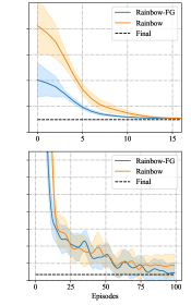
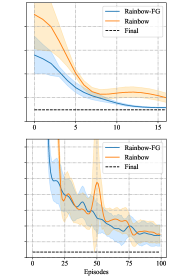
Figure 4 shows the learning process of Rainbow and Rainbow-FG with different exploration parameters in more settings. The learning processes in these settings show similar properties in section 4.3.
12 Hyperparameter Analysis
12.1 Feedback Graph Size
Theoretically, we should get enough side experiences by considering every term of and to get the largest size of . However, in practice, the time or resources may be limited so that only part of the side information can be obtained. Based on this question, this section focuses on the effect of different sizes of the feedback graph.

The default setting only constructs the feedback graph considering the current inventory , which is the first term of , and action . Each comparison group adds one following term of when constructing the feedback graph. Figure 5 illustrates the learning process of Rainbow-FG with different sizes of FG. The result shows that the sample efficiency is more sensitive to the size of FG at the initial stage than at the final stage. As the size of FG increases, the improvement of the sample efficiency mainly occurs at the initial stage. At the final stage, Rainbow-FG w/ s[0:1] & a and s[0:4] & a first reach the final level and then follows Rainbow-FG with s[0:3] & a.
12.2 Intrinsic Reward Weight
To test the sensitivity of our intrinsic reward design, we test our method with different intrinsic reward weights. Figure 6 shows the detailed learning process. A larger intrinsic reward weight tends to have higher sample efficiency during the initial stages of training. This result demonstrates the benefits of improving sample efficiency for the intrinsic reward method. However, large intrinsic reward weights can affect the performance of the final stage. The main reason is that adding the intrinsic reward to the extrinsic reward changes the original objective to be optimized.
