Model-based Design Tool for Cyber-physical Power Systems using SystemC-AMS

Abstract

Power grids have evolved into genuine cyber-physical systems (CPS) due to the increasing need for computational and communication components integrated with controlled physical systems to implement novel functions and increased resilience & fault-tolerance. These systems use computational components and real-time controllers to meet power requirements. Microgrids, composed of interconnected components, energy resources with set electrical boundaries, computational components, and controllers, provide a solution for incorporating renewable energy sources and ensuring resiliency in electricity demand. Simulating these CPS is crucial for grid design as it allows for the modeling and control of continuous physical processes along with discrete-time power converters and controllers. This paper presents a model-based design approach for creating microgrids using SystemC-AMS, which allows for physical modeling using native components defined in the SystemC-AMS library as well as user-defined computational components. Our study explores the trade-off between latency in CPS components and the sampling time required for high-fidelity simulation. We find that SystemC-AMS successfully produces the electromagnetic transient response necessary for studying grid stability. Additionally, its C-based nature allows for the integration of external libraries for added real-time capability and optimization functionality. We present three use cases to showcase the effectiveness of SystemC-AMS-based simulation.

I Introduction

Distributed and renewable energy resources to meet electricity demand have changed the landscape of the power grid. Modern power grids constitute several computational and communication components integrated with digital controllers making them suitable to study as Cyber-physical Systems (CPS). To address the environmental and economic concerns, we adopted electricity generation via renewable energy sources such as photovoltaics (PV), wind turbines, and biomass. Renewable energy sources bring an additional concern of unpredictability from the supply side which adds additional engineering requirements to be met in order to work in-situ with the main grid to serve communities [bird2013integrating]. Microgrid, a small localized version of the power grid, is created that uses distributed and/or renewable energy resources to meet electricity demand in the event the main grid is compromised due to a number of situations such as grid failure, cyber-attack, etc. In a grid-connected mode when a microgrid can send power to the main grid if there is a surplus, the microgrid has added additional requirements to improve stability and flexibility by grid operators.

Given that installing a microgrid is logistically challenging and costly, direct installation without studying in computer simulation may not lead to optimal outcomes. A number of software exist for microgrid simulation that provide varying levels of capability such as economic dispatch, secondary control, primary control, and electromagnetic transient (EMT) study [alzahrani2017modeling].

Economic dispatch simulation may not require a detailed model of microgrid components, however, conducting an EMT simulation requires a detailed modeling that may include physical circuit modeling as well as mathematical models. In this paper, we adopt a model-based engineering design approach to create grid components. These components are abstractions of physical models such as an electrical circuit representing transmission lines, resistors, capacitors, etc., and mathematical models such as a transfer function representing a low-pass filter, and subsystems such as a phase-locked loop, etc. While physical models are continuous in nature, their behavior is directly impacted by the discrete nature of the controllers. Hence, it requires careful orchestration of simulation parameters to provide high-fidelity CPS simulation. The main contribution of this paper is to create abstracted components for microgrid simulation in SystemC-AMS, an analog and mixed-signal extension of the widely popular SystemC library. We study the relationship between physical processes and timing properties of the simulation and the controller used. We demonstrate the use of SystemC-AMS to create a grid-following inverter for PV to track reference power based on a given load. Additionally, we provide a use case of a real-time simulation based on SystemC-AMS that can facilitate hardware-in-the-loop simulation.

II Background Review on Model-based Design for Cyber-physical Power Systems Modeling

The use of model-based design for modeling and simulating Cyber-physical Power Systems (CPPS) is a recent phenomenon attributed to the inclusion of communication and computational components to make grid operation resilient and fault-tolerant. Most of the work that has been done in power systems modeling doesn’t take into account the simulation aspects of cyber-physical systems. Electrical Power System Modelling in Modelica [mattsson1998physical] is one of the earlier works that led to some Modelica packages such as Spot, ObjectStab, and PowerSystems Library [winkler2017electrical], OpenIPSL [baudette2018openipsl]. OpenIPSL supports phasor time-domain simulation. Modelica is useful as it supports objected-oriented programming, and is a widely popular multi-domain modeling language for cyber-physical systems. In [cui2020hybrid], authors propose a symbolic-numerical hybrid model for the simulation of power systems. Their work has led to the creation of an open-source tool ANDES from writing models from block diagrams using predefined blocks that further generate Python code using the symbolic Python library. Another library written in C++ is DPSIM [mirz2019dpsim] which performs dynamic phasor-based simulation for power systems. However, DPSIM doesn’t provide an ability to write custom components or controller models and simulation is limited to only components available in the library. In [haugdal2021open], authors present DynPSSimPy which is able to simulate small to medium-sized grids using Python. DynPSSimPy is designed for reproducibility and expandability rather than speed of execution and accuracy.

When modeling power systems for simulation as a CPS, we need to consider a tight interaction between physical modeling and discrete-event simulation for controlling required signals to meet desired objectives. For CPPS, as we see increased usage of power electronic converters in grid design, we need to model electromagnetic transients (EMT) that require conducting a simulation with very high accuracy and at a much smaller time-step to observe the necessary transients. Using Modelica [llerins2022modelling], researchers have modeled power system simulation to produce EMT. With Modelica-like tools, the challenge remains in terms of extensibility, learning curve, and integration with other existing tools. Python-based tools suffer from the speed of execution and generally lack hardware-in-the-loop simulation support.

In addition to EMT simulation, a simulation tool should be able to provide the ability to create custom models for controllers as well as physical components. With SystemC and SystemC-AMS, we can not only model power systems and microgrid components but also, as it is written in C++, a vast number of C++ libraries can be used alongside SystemC code to provide added functionality. Further, we are looking to incorporate power electronic components at varying levels of fidelity – from physical modeling using electrical circuit components to mathematical models using discrete transfer functions or state-space equations. As such, we find SystemC-AMS suitable for modeling power systems using physical components such as resistors, capacitors, and controlled current generators in addition to modeling using transfer functions and state-space equations. Besides, we can also model software and embedded system components with SystemC which is not available with any of the tools discussed earlier [hartmann2009modeling].

SystemC [IEEE16662023] uses the discrete-event model of computation and utilizes delta-cycle to achieve deterministic simulation results. Delta cycles are non-time-consuming time-steps that consume zero time in simulation after a preceding event. SystemC-AMS, a supplemental library in C++, provides the ability to model analog and mixed-signal components and performs simulation using the SystemC simulation kernel.

In this paper, we present how we use a Model-based Design approach to create power systems components for microgrids, as well as controllers using SystemC-AMS. The main contribution of this work is the use of SystemC-AMS to create CPPS simulation by employing model-based design. We use the COSIDE tool [coside] that allows the use of a low-code, graphical drag-and-drop approach for creating SystemC and SystemC-AMS-based components that can be put together to create a CPPS such as a microgrid. We can create a time-domain simulation by specifying test cases to study the grid’s stability under multiple scenarios as well as for EMT.

In the next few sections, we explain how SystemC-AMS can be used to create physical models for power systems and provide a description of common components used for power converters and controllers in a microgrid. In later sections, we provide the use case of electrical circuits and microgrid design and explore how to design a suitable simulation scenario to produce electromagnetic transients with sufficient fidelity. We also provide a use-case with a real-time simulation scenario using an ideal DC microgrid with constant resistive load.

III SystemC Simulation Kernel and SystemC-AMS for physical modeling and controller component modeling

SystemC, a library and an event-driven simulation kernel in C++, was created to ease the design of the semiconductor intellectual property core by abstracting different levels of design. SystemC is used to model components at the system level by using networking of communicating processes. In addition, SystemC-AMS is an IEEE-1666 standard with the most recent update released in 2023 [IEEE16662023]. With SystemC, it is possible to model hardware and software jointly. On top of that, SystemC provides the possibility of carrying out the simulation of the description. SystemC integrates within it its own simulator which is an event simulator. Although concurrency is not supported in C/C++ and there is no notion of time, SystemC provides a model of time, hardware data types, module hierarchy, communication management, and concurrency. SystemC’s core provides models to represent time and provides a mechanism to obtain current time, modeling delays, and specific latency. Latency can be used to model the propagation time of information in hardware.

SystemC permits the creation of structural designs using modules, ports, and channels/signals. All ports and signals are declared to be of specific types. They facilitate data communication between modules. Modules can implement any desired functionality through processes. They are designed for concurrency. Figure 1 illustrates the relationship between SystemC modules, ports, and signals.

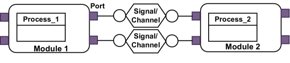
Figure 1: A diagram to illustrate modules, ports, signals, and processes in SystemC.

SystemC-AMS is an extension of SystemC that uses SystemC’s simulation kernel to model and simulate analog and mixed signals and systems that may include digital and analog filters, analog linear elements, and digital control algorithms characterized by sampling time. SystemC-AMS has multiple models of computation (MoC) for a variety of domains. Timed-data Flow (TDF) model can be used to model discrete-time processes and can be used to implement discrete transfer functions and custom algorithms. Linear Signal Flow (LSF) MoC implements some standard functionality in the continuous domain such as integrator, differentiators, delay, etc. Electrical Linear Network (ELN) MoC electrical networks use predefined elements such as resistors, capacitors, inductors, etc. With ELN MoC, we can create physical circuit models.

IV Proposed Framework for Modeling CPPS

To create components for microgrids in SystemC-AMS, we use a model-based design tool called COSIDE [coside]. COSIDE provides low-code or no-code drag-and-drop support for primitives (i.e. SystemC-AMS predefined basic components) and any user-defined modules to create a CPPS visually. COSIDE generates SystemC and SystemC-AMS C++ code skeletons for TDF MoC while for ELN MoC, it generates read-only SystemC code. Users can edit the generated TDF code and implement their logic in the processing function of TDF modules. ELN primitives can be dragged and dropped from a library on a schematic editor to construct a subsystem or a system which can be reused in other schematic editors for creating complex systems.

In order to model a CPPS, we are required to identify electrical components, any controllers, for example, phase-locked loop, environmental characteristics, identifying parameters, determine the maximum latency of any components in the system, and simulation step that can afford the maximum latency before the results can be propagated across channels from one module to another.

IV-A Physical-modeling through ELN MoC

SystemC-AMS provides current and voltage source primitive modules to model a physical current and voltage source that are of a continuous-time nature. In addition, a controlled current and voltage source can be defined that takes input from a discrete-time TDF module (see Section IV-B). An example circuit representing a physical model is illustrated in Figure 2. Each component can be dragged and dropped on the empty workspace in the COSIDE editor. The editor generates a SystemC module, a class declaration for which is provided in Listing 3. The function architecture specifies how components of the circuit are connected with each other. We skip the rest of the code for brevity (and will be made available open-source with the accepted version of the paper). The defined circuit is abstracted as a library component (as shown in Figure 4) that can be reused as a subsystem.

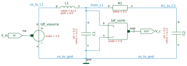
Figure 2: A circuit schematic illustrating a physical model using ELN MoC. The voltage source receives a discrete-time signal as an input from a TDF block. We measure the output as the voltage across the capacitor $C1$ using another ELN primitive voltage sink which acts as a voltmeter. Input and output ports are shown as elongated pentagonal boxes, labeled IN and OUT. The overall circuit with input/output ports can be abstracted as shown in Figure 4.

⬇ SC_MODULE(EMT_Circuit) { /// ports sca_tdf::sca_out<double> V_c; sca_tdf::sca_in<double> V_in; /// parameters struct params { double SIM_STEP; /** Simulation Step */ unsigned int T_RES; /** Time Resolution */ double L1; /** Inductance in Henry */ double C1; /** Capacitance in Farad */ double R1; /** Resistance in Ohm */ double C2; /** Capacitance in Farad */ params() { SIM_STEP = 0.000017067; T_RES = sc_core::SC_MS; L1 = 0.0022; C1 = 5.1200e-06; R1 = 0.1; C2 = 1.0240e-05; } } p; void architecture(); EMT_Circuit(sc_core::sc_module_name, const params& pa = params()); virtual ~EMT_Circuit(); struct components; components* c; components* operator -> () { return c; } }; C++ Declaration of SystemC module corresponding to the circuit shown in Figure 2. C++ structure components specifies components of the circuit, and the function architecture specifies how the terminals of each component are connected with each other.

Figure 4: An abstraction of Figure 2 that can be reused as a subsystem.

IV-B Discrete-time models through TDF MoC

The TDF MoC is capable of modeling discrete-time systems and conducting corresponding simulations, eliminating the need for costly dynamic scheduling required by SystemC’s discrete event kernel. TDF modules, when interconnected, establish a static schedule that forms a TDF cluster. This static schedule outlines the execution sequence, determines the number of samples to be read from or written to an input or output port, and sets delays at ports. These port delays are instrumental in resolving algebraic loops in feedback systems and can also simulate sensing delay. They can be further abstracted and reused to create hierarchically complex systems in a similar manner as depicted in Figure 4 with input and output ports connected to other subsystems with user-defined parameters at the design time.

V Simulation Results

In this section, we use SystemC-AMS and the model-based design framework discussed earlier on a few use cases such as the circuit discussed in Figure 2 for demonstrating EMT in an open-loop system, a grid-following inverter – a key component of a microgrid, and a secondary control for a DC microgrid model with constant resistive load showing the real-time simulation using ZeroMQ.

V-A Electromagnetic Transients in the Simulation for Open-loop System

The electrical circuit shown in Figure 2 is an equivalent electromagnetic transient model of a wye-connected, solidly-grounded three-phase transformer with two capacitor banks [watson2003power, zhao2019electromagnetic, su2012electromagnetic]. Referencing the circuit in Figure 2, connecting the two capacitors in parallel leads to a rapid transfer of charge between them. The time constant associated with this transfer is

$$\begin{split}\tau=R\bigg{(}\frac{C_{1}C_{2}}{C_{1}+C_{2}}\bigg{)}=3.35\times 10^{-7}\textrm{~{}sec}\end{split}$$ (1)

if $C_{1}=5.12\mu F$, and $C_{2}=10.24\mu F$. The parallel capacitance, when combined with the inductance, results in a natural response at a frequency of

$$\begin{split}\omega_{0}&=\cfrac{1}{\sqrt{L(C_{1}+C_{2})}}=5440\textrm{rad/s}\\ \Rightarrow T&=\cfrac{2\pi}{\omega_{0}}=1.15~{}\textrm{ms}\end{split}$$ (2)

for the inductance value $L=2.2~{}\textrm{mH}$. The time-step in a discrete-time-step simulator for electromagnetic transient response is typically much smaller than the time period of the natural response of the circuit. This is to ensure that the simulator can accurately capture the transient behavior of the circuit. A common rule of thumb is to choose a time-step that is at least an order of magnitude smaller than the smallest time constant in the system [liu2022using, wu2023fractional]. To produce a transient, we choose the time-step of the simulation as $0.05~{}\textrm{ms}\text{~{}or~{}}50~{}\mu\textrm{s}$. Choosing an extremely small time step (in the order of nanoseconds) to produce electromagnetic transients leads to a much slower simulation but the most accurate result, as shown in Figure 5. When we conduct a simulation with a significantly reduced time step and focus on a narrow region of the input/output signals, it becomes evident that any simulation time step exceeding the time constant fails to accurately reproduce the Electromagnetic Transients (EMT), as depicted in Figure 6. The figure further illustrates that it is not necessary to perform the simulation with a time-step in the nanosecond range to observe the EMT phenomenon, as further reduction in the time-step does not confer any additional benefits. However, we do note that signals in simulation with a higher time-step (say $50~{}\mu\textrm{s}$) exhibit gradual phase shift as the simulation progresses until steady state is achieved at around $0.35~{}\textrm{s}$ (not shown in the figure) when compared to the simulation with a smaller time-step (say $20~{}\textrm{ns}$) as you can observe in the signal plot for voltage measurement across the capacity bank $C_{1}$ in Figure 6. We find that this issue is not of concern for a feedback-loop-based system where a controller is designed to correct the tracking of a reference signal and the main purpose of the simulation centers around tackling high-frequency transients and a slight phase shift doesn’t obstruct such a study.

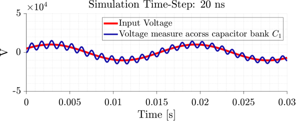
Figure 5: EMT phenomenon observed in the voltage measured across Capacitor bank $C_{1}$ from the circuit in Figure 2 when simulated in SystemC-AMS with the time-step of $20~{}\textrm{ns}$. The transient eventually disappears at around $0.35~{}\textrm{s}$ (not shown in the figure), and the voltage across the capacity $C_{1}$ stabilizes.

Figure 6: EMT phenomenon observed in the voltage measured across Capacitor bank $C_{1}$from the circuit  2 when simulated in SystemC-AMS with several different time-step values. Simulation with a large time step fails to produce an EMT phenomenon while a simulation with a time step smaller than the time period of the natural frequency exhibits an EMT phenomenon.

V-B PV-based Grid-following Inverter Design for Microgrid

Grid-following (GFL) control is widely used in grid-connected inverters, allowing the inverter to act similar to a current source. The main objective of a GFL inverter is to align with and monitor the frequency of the grid while operating as a regulated current source at a specified power output. It is engineered to supply the required amount of active and reactive power to the primary grid. GFL inverters have the ability to maintain almost steady output currents or power output during fluctuations in load. This regulation of active and reactive power is accomplished by observing the voltage of the grid, implementing a Phase-Locked Loop (PLL) [dong2014analysis, kamal2018three], and a current control loop, which facilitates swift control of the GFL’s output current.

The standard method for executing a linear controller in a three-phase system employs a PI controller operating within a dq-synchronous reference frame. This setup includes two separate control loops that manage the direct and quadrature components. However, most commercially available dynamic stability simulation tools model grid-following inverters as adjustable current sources, disregarding the inner control loops [nrel2014PSCADmodelforPV, PSSE]. This research treats GFL inverters as photovoltaic (PV) units, depicting the inverter side with an adjustable three-phase current source combined with a parasitic resistance and a high-value snubber capacitance. This configuration is designed to absorb and dissipate high-frequency oscillations, minimize overshooting, and enhance the inverter’s overall transient response [xue2022siemens, du2021GFLGFM].

Figure 7: Simplified GFL inverter without inner current loops. To break the algebraic loop that arises due to feedback, we use a delay unit $z^{-1}$ which introduces the port delay by one sample at the respective output port. LPF stands for low-pass filter. The GFL inverter model is abstracted as PV-GFL and works with the main grid as shown in Figure 8. abc 2 dq0 block is a TDF module that converts a time-varying three-phase signal to a dq0 reference frame (where signals appear to have a constant phase). dq0 2 abc does the opposite job. A PI block is a discrete-time controller implemented using TDF MoC with a sampling frequency of $1000~{}\textrm{Hz}$. We can specify active power reference and reactive power reference for the simulation as time-domain functions which are implemented using TDF MoC.

In the $dq$ reference frame, to control, aligning the $d$-axis with the space phasor of the plant model is crucial [IravaniBook]. The PLL aims to lock the GFL into the grid’s frequency or phase through a feedback implementation that nullifies the $q$-axis component of the inverter output voltage, $V_{sq}$. Consequently, the $d$-axis component of the inverter output voltage, $V_{sd}$, equals the RMS output voltage, $\hat{V}$.

$$V_{sd}=\hat{V},V_{sq}=0$$ (3)

The GFL’s control objective is to manage the real power, $P_{s}$, and the reactive power, $Q_{s}$, injected into the grid from the inverter.

$$\begin{split}P_{s}(t)&=\frac{3}{2}[V_{sd}(t)i_{d}(t)+V_{sq}(t)i_{q}(t)]\\ Q_{s}(t)&=\frac{3}{2}[-V_{sd}(t)i_{q}(t)+V_{sq}(t)i_{d}(t)]\end{split}$$ (4)

Given that $V_{sq}=0$,

$$\begin{split}P_{s}(t)&=\frac{3}{2}V_{sd}(t)i_{d}(t)\\ Q_{s}(t)&=-\frac{3}{2}V_{sd}(t)i_{q}(t)\end{split}$$ (5)

From these equations, we derive separate current references in the $dq$ domain,

$$\begin{split}i_{d,ref}(t)=\frac{2}{3V_{sd}}P_{s,ref}(t)\\ i_{q,ref}(t)=-\frac{2}{3V_{sd}}Q_{s,ref}(t)\end{split}$$ (6)

where $ref$ notation is used for reference signals.

In this paper, we discuss a simplified GFL inverter without inner current loops. Commercial dynamic simulation software typically models GFL inverters as controllable current sources, excluding the inner current loops. In the absence of the inner current loop, the control scheme mainly comprises the outer power loop, which produces the current references for the controllable current sources. A simplified block diagram of the GFL inverter, devoid of inner current loops, is depicted in Fig. 7.

The active and reactive power, denoted by $P$ and $Q$, are measured in the $dq$-reference frame as per Eq. (4) and subsequently filtered using a discrete low-pass filter to eliminate high-frequency elements in power measurement. The bandwidth of this low-pass filter can be further utilized to incorporate an inertial response from the inverter [Poolla2019FFR]. The $d$ and $q$ axes are uncoupled, thereby enabling independent control over $P$ and $Q$. However, due to the EMT phenomenon, we see some effect of step-change in active power on the reactive power. The measured power is then subtracted from the references, $P_{\textrm{ref}}$ and $Q_{\textrm{ref}}$, and passed through a PI controller that monitors the deviation of active and reactive power from the set reference to stabilize the instantaneous active and reactive power.

Figure 8: A PV-GFL inverter acting as a microgrid that works with the main grid. The main grid is modeled as a three-phase voltage source connected through the transmission line. Three-phase controlled current source is a group of three controlled current source elements provided by the SystemC-AMS library that act as a current source based on the input value. VI measurement block consists of a voltmeter and an ammeter (called voltage sink and current sink in SystemC-AMS) that measure voltage and current respectively. The overall implementation also provides three-phase grid voltage $V_{g_{a},g_{b},g_{c}}$ and current $I_{g_{a},g_{b},g_{c}}$ as output that can be logged during the simulation.

We can use the PV-GFL design for constructing a microgrid and its interaction with the main grid. The use of PV-GFL for operating with the main grid is depicted in Figure 8. PV-GFL model receives three-phase voltage $V_{a,b,c}$ and three-phase current $I_{a,b,c}$ as inputs and outputs regulated current $I_{aPV,bPV,cPV}$ as output. Figure 8 has an ideal grid modeled as a three-phase voltage source connected through a transmission line. The transmission is modeled as a lossy transmission using resistance in series with inductance. The overall model comprises an algebraic loop which can be broken by introducing a delay unit $z^{-1}$ (where is $z$ variable is from z-transform) in the GFL inverter model as shown in Figure 7. We measure the instantaneous active and reactive power $P$, and $Q$ using three-phase voltages $V_{a,b,c}$, and currents $I_{a,b,c}$ using the formula from Equation (7) as follows:

$$\begin{split}P&=V_{a}I_{a}+V_{b}I_{b}+V_{c}I_{c}\\ Q&=\cfrac{1}{\sqrt{3}}\bigg{(}(V_{a}-V_{b})I_{c}+(V_{b}-V_{c})I_{a}+(V_{c}-V_{a})I_{b}\bigg{)}\end{split}$$ (7)

To conduct the simulation in SystemC-AMS, we use a simulation time-step of $50~{}\mu\textrm{s}$ and run the simulation for $10~{}\textrm{s}$. The three-phase voltage source has the root-mean-square phase-to-phase voltage of $480$ V operating at $60$ Hz. The transmission line [chew2020lectures] is modeled as a series resistance of $0.01~{}\Omega$, a series inductance of $0.0001~{}H$, a shunt resistance of $0.15~{}\Omega$, and shunt capacitance of $80~{}\mu F$. Three-phase load is a pure resistive load of $1000~{}\Omega$. The low-pass filter (LPF block in Figure 7) uses the z-domain transfer function $\tfrac{0.0609}{z-0.9391}$ at the sampling rate of $1000~{}\textrm{Hz}$. Phase-locked-loop (PLL block in Figure 7) establishes a relationship between grid voltage and frequency. A GFL inverter uses PLL to keep the inverter in synchronization with the main grid. The measured angle is used to control the current. We study the step response by providing several step-change inputs that act as references for reactive and active power. We observe electromagnetic transients in the reactive power in response to the change in the active power as shown in Figure 9. Finally, we also compared the implementation of the GFL inverter design in SystemC-AMS with one in Simulink and our implementation demonstrated that SystemC-AMS provides three times faster simulation compared to Simulink-based simulation.

(a)

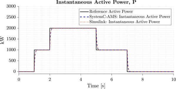
(b)

Figure 9: Simplified GFL inverter without inner current loops: step response. Top: Instantaneous reactive power plot with SystemC-AMS simulation of GFL inverter-based microgrid. We zoom in around the first transients as you can see in the inset figure. We also plot the reference reactive power. Bottom: Instantaneous active power plot in SystemC-AMS simulation. Notice the electromagnetic transients in reactive power as there is a step change in the active power – thereby demonstrating the capability to simulate EMT.

V-C Real-time Simulation of a DC Microgrid Model with Constant Resistive Load

In another case study, we decouple the controller from the microgrid plant to facilitate a real-time simulation. We use a DC microgrid with a primary control and a secondary control where the DC microgrid along with the primary control acts as a plant while the secondary control is a separate model communicating with the plant through ZeroMQ communication API [hintjens2013zeromq]. We model a single-bus DC microgrid consisting of a DC-DC converter, an inductor, a capacitor, and a load [tu2023impact] (see Figure 10). The inductor and capacitor together are equivalent to the line impedance, filters, and DC bus capacitor.

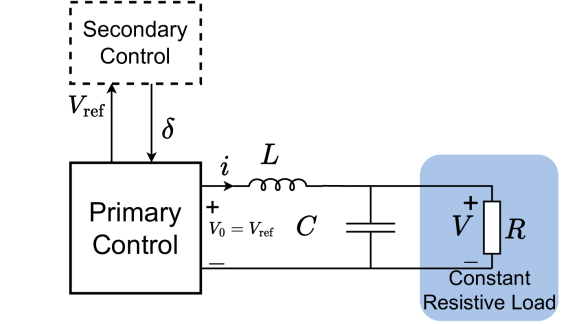
Figure 10: The model of a DC microgrid with a steady resistive load is considered. The primary controller, known as the droop controller, sets the reference voltage using a nominal voltage and the output current. If needed, a secondary controller can be employed to fine-tune the nominal voltage set by the primary controller in order to control the voltage of the microgrid, with an extra correction term $\delta(t)$.

The equation describing the DC microgrid is

$$\begin{split}V_{\text{ref}}(t)-V(t)&=L\cfrac{di}{dt}\\ i(t)-\cfrac{V(t)}{R}&=C\cfrac{dV}{dt}\end{split}$$ (8)

where $i$ is the inductor current; $V$ is the capacitor voltage; $V_{0}$ and $V_{\text{ref}}$ are the converter’s output voltage and reference voltage, respectively. We also assume that the output voltage can track the reference voltage as accurately as possible due to the converter’s inner current loop which is $V_{0}=V_{\textrm{ref}}$. $V_{\textrm{ref}}$ is generated by a primary controller (a droop controller) as follows

$$\begin{split}V_{\text{ref}}(t)=V_{n}-k\cdot i(t)\end{split}$$ (9)

where $k$ is the droop gain, and $V_{n}$ is the nominal voltage. Any fluctuation in the current $i(t)$, due to the constant resistive load, directly affects the reference voltage $V_{\text{ref}}$. In order to keep the voltage of a droop-controlled DC microgrid at its nominal level, a secondary controller can be implemented. This controller adjusts the nominal voltage $V_{n}$ using a correction term $\delta(t)$. In the context of this article’s use case, both the primary and secondary controllers are regulated by the subsequent equation:

$$\begin{split}V_{n}^{\prime}(t)&=\delta(t)+V_{n}\\ V_{\text{ref}}(t)&=V_{n}^{\prime}(t)-k\cdot i(t)\\ \delta(t)&=\int k_{s}(V_{n}-V_{\text{ref}}(t))dt\end{split}$$ (10)

where $k_{s}$ is the secondary control gain. Secondary controllers typically operate at a frequency ranging from 1 to 100 Hz [Tu2020], a rate that is compatible with real-time execution using SystemC-AMS. We set the nominal voltage of $V_{n}=200~{}\textrm{V}$, $k=0.2$, and $k_{s}=0.75$.

A schematic of our approach for real-time simulation is shown in Figure 11.

Figure 11: A microgrid simulation with the plant and controller exchanging data through a communication interface. In the context of this paper, we use ZeroMQ for communication.

As SystemC-AMS is designed for fast simulation, only limited by the device’s capability, we create a customized TDF module called the relay module that uses ZeroMQ API to schedule the message exchange between the plant and the controller using ZeroMQ subscribers and publishers. The module corresponding to the controller and the plant measures the computation time to produce the new result that is propagated by the relay modules. The relay modules deliver the new result to the other party only if time corresponds to the step size of the simulation that has elapsed since the start of the new calculation. Note that in this case, real-time simulation is only possible if the time required to perform a calculation by a SystemC-AMS module is less than the specified step size of the simulation. In addition to using ZeroMQ, we use PREEMPT_RT kernel patch in the Ubuntu and execute the binaries corresponding to the simulation with the highest scheduling priority. A schematic of the implementation is illustrated in Figure 12. Please refer to a paper [bhadani2023wsc] for additional details on this topic.

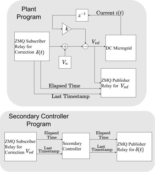
Figure 12: A diagram of the DC microgrid features a primary controller, along with ZeroMQ subscriber and publisher relay modules. The subscriber relay module retrieves data from the secondary controller, logging the timestamp of the data retrieval. This information is then passed to the publisher relay module. Using the most recent timestamp and the elapsed time, the publisher relay module calculates the necessary wait time to simulate real-time behavior. Additionally, an algebraic loop is prevented by incorporating a delay unit.

The plant simulation was carried out with a time step of 1 ms, whereas the secondary controller operated with a time step of 100 ms. These values are representative of how the primary controller (a part of the plant) and the secondary controller operate in the real world. Looking at Figure 13, the output voltage $V_{0}$ is measured as the adjusted reference voltage from Equation (10) and starts at $200~{}V$ (shown in the top subplot of Figure 13). However, it fails to maintain the nominal value due to fluctuation in the current caused by the resistive load. The secondary controller compensates for the decrease in the output and over time voltage stabilizes to the set nominal voltage. During its operation, the plant keeps the old value of the signal until receives a new value from the secondary controller. Such real-time simulation is also useful when the secondary controller is implemented by some other program or in fact it can be a hardware implementation to allow hardware-in-the-loop simulation. Initially, the plant may execute in an open-loop manner and once the controller is online, it is expected to stabilize the plant if designed correctly. To study such behavior, we induce the delayed start of the controller. In the absence of the controller, the reference voltage doesn’t reach the specified nominal voltage of $200~{}\textrm{V}$. When the secondary controller is executed with a delayed start, the settling time is achieved at a later time. When the start is delayed by $0.1$ s, the reference voltage’s settling time is $0.986$ s. If the start is delayed by $0.5$ s, the settling time becomes $1.383$ s, and with a delay of $2.0$ s in the start, the settling time is observed to be $2.869$ s. The result from this simulation is plotted in Figure 13.

Figure 13: Simulation results of a DC microgrid, where the primary controller acts as a plant in a SystemC-AMS simulation, are presented. These results include voltage traces and the correction term $\delta(t)$. The output voltage $V_{0}$ which is measured as the adjusted reference voltage from Equation (10) starts at $200~{}V$ (shown in the top figure), but it falls due to fluctuation in the current caused by the resistive load. The secondary controller compensates for the decrease in the output and over time voltage stabilizes to the set nominal voltage. Different scenarios of secondary controller execution are demonstrated, starting with a scenario where it is completely absent. For each case of $0.1$ s, $0.5$ s, and $2.0$ s delay, we zoom in on a segment between $0.2$ s to $7.0$ s of the voltage plot in the inset on the top subplot (marked with a box on the full plot). We observe that the voltage stabilizes later if the secondary controller comes online with some delay. Note that the x-axis is log-scaled.

To assess the efficacy of real-time simulation, we also logged the time-stamp of the reference voltage message published by the ZeroMQ relay module. The DC microgrid plant simulation was configured with a time-step of $1$ ms. In a perfect real-time system, we would anticipate the average time difference to be $1$ ms with no standard deviation. However, the simulation data revealed that the median time difference was $1.01259$ ms, the average was $1.01728$ ms, and there was a standard deviation of $0.08753$ ms. A Histogram of the message interval is provided in Figure 14.

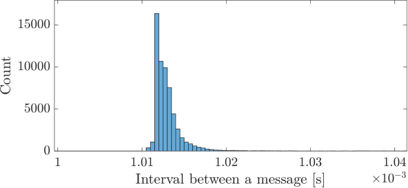
Figure 14: Histogram showing intervals between the timestamps of message publications.

VI Conclusion and Future Discussion

In this paper, we have presented our work on the model-based design of microgrid components using SystemC-AMS, constructing a DC microgrid, and a microgrid design using GFL inverters. We conducted a simulation study of GFL with an ideal main grid. Our approach demonstrated that SystemC-AMS can perform a fast simulation, exhibits EMT phenomenon, and can interface with external libraries. Additionally, we introduced a real-time simulation method that incorporates a communication component, using the ZeroMQ C++ library for message exchange between the plant and controller simulations. This strategy allows SystemC-AMS to function as a digital twin for microgrids, facilitating hardware-in-the-loop experiments with hardware prototypes to refine control algorithms. Our future work involves expanding grid components in SystemC-AMS to study microgrids at scale and demonstrating the capabilities of real-time simulation in conjunction with hardware components to regulate grid signals under various conditions. In the follow-up of the current work, we will test the SystemC-AMS implementation of a microgrid with middleware control applications implemented in RIAPS [ghosh2023distributed, eisele2017riaps].