Quantum hall transformer in a quantum point contact over the full range of transmission

Abstract

A recent experiment [Cohen et al., Science 382, 542 (2023)] observed a quantized $e^{2}/2h$ conductance tunneling into a fractional quantum hall edge in the strong coupling limit, which is consistent with the prediction of a quantum Hall transformer. We model this quantum point contact (QPC) as a quantum wire with a spatially-varying Luttinger parameter and a back-scattering impurity and use a numerical solution to find the wavepacket scattering and microwave (i.e. finite frequency) conductance at the interface. We then compare the microwave conductance to an analytic solution of a Luttinger liquid with an abruptly varying Luttinger parameter and a back-scattering impurity, which is obtained by mapping the problem to a boundary sine-Gordon (BSG) model. Finally, we show that the quantum Hall transformer can survive the inclusion of the domain wall that is expected to occur in a wide QPC, which is experimentally relevant, provided the momentum change in the QPC is generated by electrostatics. We find that back-scattering generated by the domain wall is of an order of magnitude consistent with the experiment.

I Introduction

Fractional quantum Hall (FQH) systems are one of the few experimentally known platforms that are expected to support chiral Luttinger liquid edge states [1]. Interestingly, a recent experiment [2] in graphene FQH quantum point contacts (QPCs) has seen differential conductance that closely matches theoretical predictions [3, 4, 5] (both low voltage and temperature power-law scaling as well as high voltage universality) based on the boundary sine-Gordon (BSG) model [6]. Such quantitative experiments, if described by the BSG, open more vistas into its physics, which can include rather intricate phenomena [6] accessed in relatively few experiments [7]. Interestingly, the high voltage universal regime of the BSG model, where the differential conductance is near a quantized value of $e^{2}/2h$ [2], realizes a dc voltage transformer, i.e. the quantum Hall transformer (QHT) [5].

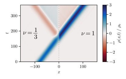
Figure 1: Sign-flipping reflection of a charge wavepacket from the interface between $\nu=1/3$ and $\nu=1$ quantum Hall edge states, illustrating the quantum hall transformer behavior. The charge is normalized by a factor $\rho_{0}$ to illustrate the $2e^{*}\rightarrow-e^{*},\;3e^{*}=e$ charge transfer. The constant charge near the interface at late times agrees with the sensitivity of the low frequency ac conductance to imperfections in the interface (see Fig. 2).

Despite the agreement with the BSG model, the microscopic connection between this model and the experiment remain unclear. The interpretation of the BSG model as a tunneling term between chiral LL edges of $\nu=1/3$ and $\nu=1$ FQH states [3] is complicated by the irrelevance under the renormalization group [8] of such a perturbation and the large width of the QPC in experiments [2]. This raises the possibility that a more complex multi-tunneling model [9] as a model for the experiment. Similarly, a resonant impurity in the FQH state, which can realize such a strong tunneling [4], is also likely to depend on details, though resonances in the measured transmission [2] provide some motivation for this model.

A configuration for generically creating strong coupling [5] (i.e. the QHT limit), is in principle based on pinching the QPC to near the magnetic length and then adiabatically varying the density between the two FQH states at filling $\nu=1/3$ and $\nu=1$. The adiabatic contact in this theory takes the form of a conventional Luttinger liquid with the Luttinger parameters adiabatically evolving between the values corresponding to $\nu=1/3$ to $\nu=1$. Since a weak back-scattering impurity is a relevant perturbation in an LL [8, 10], this model provides a natural framework to describe a high-temperature/voltage limit with a differential conductance of $e^{2}/2h$ and a low temperature impurity dominated limit with vanishing differential conductance. However, whether such a model can describe the experiment [2], which is not in the narrow QPC limit, is also unclear.

In this work, we provide an alternative (relative to Ref. 3) interpretation of the BSG model [6]—as arising from an impurity in the above Luttinger liquid model [5]—to understand the quantitative conductance in the weak and strong impurity limit. We do this by comparing the numerically computed ac conductance of a model of a Luttinger liquid with an impurity and a spatially varying Luttinger parameter to the ac conductance of the BSG model. This allows us to relate the effective back-scattering in the BSG model with the microscopic parameters in the Luttinger model. Finally, we discuss models of a wide QPC that can be described by the Luttinger model where the scattering from the domain wall can provide the back-scattering in the BSG.

II Luttinger liquid model

The Hamiltonian for an impurity in a Luttinger liquid [8], assuming the density variation back-scattering [10] to be of strength $g$ at $x=0$, can be represented by the Hamiltonian

$$H=\int\mathrm{d}x\frac{v(x)}{2\pi}\left[K(x)\Pi^{2}+K(x)^{-1}(\partial_{x}\phi)^{2}\right]-g\cos{2\phi(0)},$$ (1)

where the boson field $\phi$ is defined in terms of the charge density $\rho=-\pi^{-1}\partial_{x}\phi$ in units of the electron charge $e$. Here $\Pi(x)$ is the momentum that is canonically conjugate ($[\phi(x),\Pi(x^{\prime})]=i\pi\delta(x-x^{\prime})$) to the boson field $\phi(x)$. The pair of edges of a FQH strip at filling fraction $\nu$ has a Luttinger parameter $K(x)=\nu$ and a mode velocity $v(x)$ that matches the edge velocity, which we take to be $1$ across the junction by rescaling $x$ [3]. To represent the junction, we smoothly vary $K(x)$ in space. Conservation of charge requires that the current operator is written as $j=\pi^{-1}\partial_{t}\phi=(i/\pi)[H,\phi]=vK\Pi/\pi$. An applied voltage $V$ can be described by adding a perturbation $H_{\mathrm{ext}}=V\phi(0)$ to the Hamiltonian $H$.

In the absence of back-scattering (i.e. $g=0$), which is referred to as the quantum Hall transformer [5], the Hamiltonian in Eq. 1 is harmonic so that the conductance is independent of temperature. By approximating the $K(x)$ profile as exponential over a region of width $d$ and constant otherwise, and using the Kubo formula for the response of the current $j(\omega)$ with perturbation $V(\omega)$, the ac conductivity is analytically solvable, yielding

$$G(\omega)=\frac{e^{2}}{h}\,\frac{e^{-i\theta}\sqrt{K_{-}K_{+}}}{\cosh\Delta-i(\theta/\Delta)\sinh\Delta}$$ (2)

where $\Delta^{2}=(\frac{1}{2}\log K_{-}/K_{+})^{2}-\theta^{2}$ and $\theta=\omega d/v$. The value of $\theta$ parameterizes the width of the junction $d$ relative to the wavelength of the driven modes. This formula reduces to the quantum hall transformer dc conductivity $G\sim(2e^{2}/h)(K_{-}^{-1}+K_{+}^{-1})^{-1}$ [9, 5] as $\omega$ goes to $0$ but approaches $G\sim(e^{2}/h)\,(K_{-}K_{+})^{1/2}$ in the large frequency/long junction limit ($\omega\gg v/d$). The $e^{2}/2h$ dc conductance in this limit can be understood as the Andreev reflection-like process (see Fig. 1) where a charge packet of charge $2e/3$ is reflected to a packet of $-e/3$ with the opposite sign. This process can be understood to be a result of the conservation of chiral charge in the Luttinger liquid [11] in the absence of back-scattering since the chiral charge of the incoming and reflected packets are $K_{-}^{-1}(2e/3)=2e$ and $K_{-}^{-1}(e/3)=e$ respectively while the transmitted packet has a chiral charge of $K_{+}^{-1}e=e$.

III Numerical model ac conductance

The above result in the dc limit ($\omega\rightarrow 0$) is fine-tuned to $g=0$, since a finite strength of impurity $g>0$ is expected to be a relevant perturbation [8] and requires a numerical treatment. For this purpose, we approximate the model in Eq. 1 as an interacting fermion lattice model with next-nearest neighbor interactions [12], described by a Hamiltonian

$$H=\sum_{n}\left(t_{n}c^{\dagger}_{n}c_{n+1}+\mathrm{h.c}-\mu_{n}n_{n}\right.\\ \left.+\;U_{n}n_{n}n_{n+1}+U^{\prime}_{n}n_{n}n_{n+2}\right)+un_{0}$$ (3)

where the spatially dependent parameters correspond to $K=1$ and $K=1/3$ Luttinger liquids with a short, smooth interface. For the $K=1$ side we use $t_{n}=0.308$, $\mu_{n}=0.360$, $U=0$ and $U^{\prime}_{n}=0$ while for the $K=1/3$ side we use $t_{n}=0.122$, $\mu_{n}=0.293$, $U=0.293$ and $U^{\prime}_{n}=0.439$. This choice keeps the velocity and background magnetization approximately constant. The interface between the two sides consists of a smooth 3-site transition in each of the parameters and a single-site barrier $u$. Such a model can be transformed to a spin-1/2 XXZ model via a Jordan-Wigner mapping.

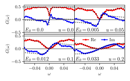
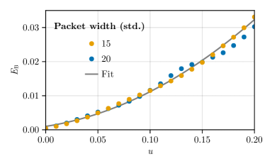
Figure 2: (top) ac conductivity for various impurity strengths $u$ and packet width $15$ demonstrating near $G=e^{2}/2h$ for $u=0$. The real part of the data is fit to Eq. 12 to calculate barrier energy $E_{\mathrm{B}}$, with fits shown as dashed lines. (bottom) Fit value of $E_{\mathrm{B}}$ as a function of impurity strength $u$, demonstrating a quadratic relationship. Data from the narrower packet is fit to $E_{\mathrm{B}}=A(u+u_{0})^{2}$, which yields $A=0.55$ and $u_{0}=0.04$, the latter of which represents the intrinsic back-scattering of the Luttinger parameter crossover.

We can probe the ac conductance of this junction using a Gaussian chiral wavepacket, generated by a local quench in the chemical potential $\mu_{n}$ and a gauge field $a_{n}$ such that $t_{n}\mapsto t_{n}e^{ia_{n}}$ [13]. We use the density matrix renormalization group [14, 15] to solve for the ground state of this quenched Hamiltonian and then use the time-evolving block decimation algorithm [16, 17] to evolve the packet in real time with a fourth-order Trotter decomposition [18]. The propagation of these packets is nearly dissipationless, since the packet is perturbatively small ($\rho\lesssim 10^{-3}$), and the transport process is clear from the the packet transmission, as shown in Fig. 1. Comparing the initial and transmitted packet in the frequency domain gives the ac conductance, plotted in Fig. 2. Note that due to the discrete geometry and the finite bandwidth of the Gaussian wavepacket, there is a trade-off between frequency range and resolution, and therefore two different packet widths are used. Numerical details can be found in the Supplementary Material (SM).

IV Boundary sine-Gordon model

The Hamiltonian Eq. 1, for $g>0$, is essentially an impurity in a Luttinger liquid, which can be solved by mapping to a boundary sine-Gordon model (BSG) [6] by folding the $x<0$ solution using a reflection $x\rightarrow-x$ [19]. Applying this transformation generates a two-component boson field $\phi_{-}(x)=\phi(-x)$ and $\phi_{+}(x)=\phi(x)$ for $x\geq 0$. The effect of a weak impurity $g$ is expected to be limited to low energy modes, whose wavelength is longer than the variation of $K(x)$. We will therefore assume the Luttinger parameter associated with $\phi_{\pm}$ to be constants $K_{\pm}$ respectively. The boundary condition for $\phi_{\pm}(x\sim 0)$ changes abruptly near $x\sim 0$, so that the boundary condition is written as $K_{+}^{-1}\partial_{x}\phi_{+}=-K_{-}^{-1}\partial_{x}\phi_{-}$.

This boundary condition couples the otherwise decoupled left and right channels. The fields decouple completely under a rescaling by $K_{\pm}^{-1/2}$ and an $O(2)$ rotation, with $\xi$ and $\bar{\xi}$ fields defined as

$$\left(\begin{matrix}\xi\\ \bar{\xi}\end{matrix}\right)=\Gamma\left(\begin{matrix}K_{-}^{-1/2}&K_{+}^{-1/2}\\ K_{+}^{-1/2}&-K_{-}^{-1/2}\end{matrix}\right)\left(\begin{matrix}\phi_{-}K_{-}^{-1/2}\\ \phi_{+}K_{+}^{-1/2}\end{matrix}\right).$$ (4)

and likewise with their conjugate momenta $\eta$ and $\bar{\eta}$ (rescaling by $K^{1/2}_{\pm}$ instead of $K^{-1/2}_{\pm}$). Here $\Gamma\equiv(K_{-}^{-1}+K_{+}^{-1})^{-1/2}$. Under this transformation, the boundary conditions become $\bar{\xi}(0)=0$ and $\partial_{x}\xi(0)=0$.

Since $\bar{\xi}$ vanishes at $x=0$, the original field at the boundary $\phi(0)$ can be written purely in terms of $\xi(0)$ as $\phi(0)=\Gamma\xi(0)$, decoupling $\xi$ from $\bar{\xi}$. The $\bar{\xi}$ equation has no boundary term and cannot affect the current, so we focus on the $\xi$ part of the Hamiltonian:

$$H_{\xi}= \int_{0}^{\infty}\frac{\mathrm{d}x}{2\pi}\,\left[\eta^{2}+(\partial_{x}\xi)^{2}\right]-g\cos{(2\Gamma\xi(0))}.$$ (5)

Writing the perturbation $H_{\mathrm{ext}}$ to the Luttinger liquid Hamiltonian Eq. 1 in terms of $\xi(0)$, we conclude that the voltage $V$ transforms to an effective voltage $V_{\mathrm{eff}}=\Gamma V$ applied to the Hamiltonian $H_{\xi}$. The total current flowing through the junction then transforms into

$$j=\Gamma\pi^{-1}\eta(0).$$ (6)

To analyze the above semi-infinite systems we combine the fields $\xi(x)$ and $\eta(x)$ into the chiral boson field ${\xi_{\mathrm{c}}}(x)=(1/2)[\xi(|x|)+\int_{0}^{x}\mathrm{d}x^{\prime}\,\eta(|x^{\prime}|)]$ on the entire real line $x\in(-\infty,\infty)$ [20]. The von Neumann boundary conditions $\partial_{x}\xi(0)=0$ ensure that ${\xi_{\mathrm{c}}}(x)$ is differentiable at $x=0$. Following Refs. 21, 22, and introducing a soft UV cutoff $a$ we refermionize the bosonic Hamiltonian by defining the chiral fermion field

$${\psi_{\mathrm{c}}}(x)=\frac{\alpha}{\sqrt{2\pi a}}\,e^{-2i{\xi_{\mathrm{c}}}(x)},$$ (7)

where $\alpha=\exp[i\pi({\xi_{\mathrm{c}}}(0)-{\xi_{\mathrm{c}}}(\infty))]$ is the fermion parity of the refermionized model. The boundary term, for the specific case $\Gamma=1/2$ (corresponding to $K_{+}=1/3$ and $K_{-}=1$), can be written in terms of this chiral fermion operator as

$$g\cos{\xi(0)}=\sqrt{2E_{\mathrm{B}}}\,\alpha\left({\psi_{\mathrm{c}}}(0)+{\psi_{\mathrm{c}}}^{\dagger}(0)\right)$$ (8)

where $E_{\mathrm{B}}=g^{2}\pi a/4$. This term is quadratic in fermion operators due to the operator $\alpha$.

The equations of motion of the fermion fields ${\psi_{\mathrm{c}}}(x)$ and $\alpha$ resulting from the above boundary Hamiltonian results in Andreev transmission [23] of ${\psi_{\mathrm{c}}}(x)$ from the operator $\alpha$ which behaves like a Majorana operator.

However, the charge of the chiral fermion ${\psi_{\mathrm{c}}}$ does not correspond to electronic charge. This issue is resolved by defining the fermion in the original interval $x\in[0,\infty]$ in terms of the chiral fermions using the relation

$$\psi^{\dagger}(x)=e^{ik_{\mathrm{F}}x}{\psi_{\mathrm{c}}}^{\dagger}(x)+e^{-ik_{\mathrm{F}}x}{\psi_{\mathrm{c}}}(-x).$$ (9)

By using this definition of the fermion operator, we can write the current in Eq. 6 as:

$$j(x)=(i/2)(\psi^{\dagger}(x)\partial_{x}\psi(x)-\mathrm{h.c.}),$$ (10)

which is the conventional form of the fermion current in a one dimensional wire. Here the wavelength for the the chiral fields is assumed to be much longer than $k_{\mathrm{F}}^{-1}=1$ (chosen to be consistent with Fermi velocity and mass being one). Using the fermion definition Eq. 9 with the corrected charge, the Andreev and normal scattering amplitudes for the fermion $\psi(x)$ can be computed from the Bogoliubov-de Gennes equations (see SM for details), similar to resonant Andreev reflection from a Majorana zero mode [23]:

$$r_{\mathrm{A}}=\frac{iE}{iE+E_{\mathrm{B}}}\quad\,r_{\mathrm{N}}=-\frac{E_{\mathrm{B}}}{iE+E_{\mathrm{B}}}.$$ (11)

At low energies $|E|\ll|E_{\mathrm{B}}|$ we see that $|r_{\mathrm{N}}|\sim 1$ (i.e. perfect normal reflection) while high energy fermions with $|E|\gg|E_{\mathrm{B}}|$, are Andreev reflected (i.e. $|r_{\mathrm{A}}|\sim 1$).

This result is consistent with previous works solving Eq. 5 using a Kramers-Wannier duality [24, 25] and conformal field theory techniques [6, 26, 27].

The voltage and temperature dependence resulting from this Andreev reflection [9, 23] is in good agreement with recent experimental results [2]. Applying the formalism of dynamic conductance [28], we find the ac conductance associated with the above Andreev reflection process to be:

$$G(\omega) =\frac{e^{2}}{2h}\left[1-\frac{E_{\mathrm{B}}}{i\omega}\,\mathrm{Ln}\left(1+\frac{i\omega}{E_{\mathrm{B}}}\right)\right].$$ (12)

The real part of the ac conductance vanishes as $\omega\rightarrow 0$, which is consistent with the irrelevance of the tunneling perturbation [8]. Furthermore, it reaches the harmonic value of $1/2$ as $\omega\rightarrow\infty$, which is consistent with Eq. 2 when $v/d\gg\omega\gg E_{\mathrm{B}}$. We fit the ac conductances in Fig. 2 with Eq. 12 and find a close resemblance at low frequencies, where the ratio of Gaussians is well defined. Furthermore, we can deduce the values of $E_{\mathrm{B}}$ for difference back-scattering strengths $g$, which is seen in Fig. 2 to be broadly consistent with the theoretical estimate apart from a shift $u_{0}$ that likely arises from the spatial variation of $K(x)$.

V Luttinger liquid as a model for the QPC

The Luttinger liquid model Eq. 1 for the quantum Hall transformer, which is based on the edge charges and currents, was originally justified for a QPC of width comparable to the magnetic length $l_{\mathrm{B}}$ [5], however this justification must be modified for the relevant experimental realization [2] where the QPC is much wider than a magnetic length. This is, however, subtle when the filling varies between the values of $\nu_{-}=1$ and $\nu_{+}=1/3$ in the middle of the QPC, resulting in a compressible domain wall shown in Fig. 3. While a detailed analysis of the low-energy structure based on numerical diagonalization or Chern-Simons theory [29] of the QPC is beyond the scope of the current work, for QPC widths smaller than $W\lesssim v_{\mathrm{DW}}/k_{\mathrm{B}}T_{0}$ and $v_{\mathrm{DW}}/V_{\mathrm{bias}}$, the domain-wall modes would effectively be gapped on a scale that is larger than the temperature $T_{0}$ and the applied bias $V_{\mathrm{bias}}$, scaling with the velocity $v_{\mathrm{DW}}$ of domain-wall excitations. One can then expect the charge dynamics to be dominated by the edges of the QPC (see the SM for more details) such that the Luttinger liquid model is a reasonable description.

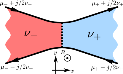
Figure 3: Schematic of a QPC between filling $\nu_{-}=1$ and $\nu_{+}=1/3$. The arrows represent the direction of movement of the electron at each edge. The dotted line represents a domain wall with effective chiral charge $\nu_{-}-\nu_{+}=2/3$ with disorder [30]. The chemical potential of each segment of edge is shown to be $\mu_{\pm}+\mathrm{sgn}(y)\,j/2\nu_{\pm}$ where $j$ is the total current flowing through the QPC and the edge velocity near the ends is chosen to be unity.

The quantum Hall transformer behavior in the conductance of the harmonic Luttinger liquid model —as proposed in Ref. 5—can be attributed to momentum-based chiral charge conservation [11]. Motivated by this argument, we explicitly consider the effect of momentum conservation to a model of the QPC with a short domain wall dominated by edge charges as shown in Fig. 3. We choose the chemical potentials of the edges to be $\mu_{-}\pm j/2\nu_{-}$ on the left-hand side of the QPC and $\mu_{+}\pm j/2\nu_{+}$ on the right side. Here $j$ is the current flowing through the QPC and $\nu_{-},\nu_{+}$ are the filling factors on the two sides. Assuming that the QPC does not generate significant noise as in the two extremes of the Luttinger liquid, the rate at which canonical momentum is carried away by the current (i.e. the total force in the $x$-direction) is simply a product of the current on each edge and the corresponding vector potential and is written as

$$F_{\mathrm{current}}=(\nu_{-}\mu_{-}-\nu_{+}\mu_{+})BW^{\prime}.$$ (13)

In the above equation, the gauge is chosen so that the vector potential at the ends of the top and bottom edges in Fig. 3 is $A=\pm BW^{\prime}\hat{x}/2$, the edge velocity at the ends is chosen to be unity and $W^{\prime}$ is the width of the QPC at the left and right ends of Fig. 3 where $\mu_{\pm}$ are measured. This momentum change is generated by the interaction of the charge density with the electrostatic potential generated by the gates, generating a force $F_{\mathrm{gates}}(\mu_{-},\mu_{+},j)$. Within linear response, one can expand this force in terms of $\delta\mu\equiv(\mu_{+}-\mu_{-})/2$ and $j$ as $F_{\mathrm{gates}}(\mu_{-},\mu_{+},j)=C_{0}+C_{1}\delta\mu+C_{2}j$ where the coefficients can depend on $\bar{\mu}\equiv(\mu_{+}+\mu_{-})/2$. The current $j$ can be determined from the momentum conservation equation

$$C_{0}+C_{1}\delta\mu+C_{2}j-(\nu_{-}\mu_{-}-\nu_{+}\mu_{+})BW^{\prime}=0.$$ (14)

Since momentum conservation must apply in equilibrium (i.e. $\mu_{-}=\mu_{+}$ and $j=0$), the constant term but be $C_{0}=(\nu_{-}-\nu_{+})\bar{\mu}BW^{\prime}$. For the special case of a QPC with mirror symmetry along the $y$ axis, we can use the mirror operator to interchange the chemical potentials on the top and bottom edges without changing the direction of the currents so that this transformation flips $j$ and preserves $\mu_{\pm}$. Applying this symmetry to Eq. 14, leads to the conclusion that $C_{2}=0$, which then forces the constraint $\mu_{+}=\mu_{-}$. The voltage in the QPC is the difference in the chemical potentials of the two incoming leads is $V=j(1/2\nu_{-}+1/2\nu_{+})$, which results in the expected conductance of the quantum Hall transformer matching $G=2\nu_{-}\nu_{+}/(\nu_{-}+\nu_{+})$ [5]. This result is explicitly demonstrated for an edge model of the QPC in the SM. The quantum Hall transformer conductance is reduced by impurity-induced large momentum elastic back-scattering. As elaborated in the SM, we find that scattering from a soliton-like structure (e.g. $\nu=2/3$ domain wall) can support a scattering matrix element in Eq. 1 that is of the correct order of magnitude to account for the recent measurements [2].

VI Conclusion

We have provided an alternative interpretation to the BSG model that is used to fit the recent experiments [2] as arising from an impurity in the Luttinger model for the QHT [5]. We have compared these results with a numerical solution of the Luttinger model to map out the correspondence between the parameters of the two models. These results also make predictions for the microwave conductivity in addition to previous results [9, 3, 25] on shot noise that could guide future studies on these QPC systems. In addition, we have shown that inclusion of momentum conservation in the dynamics of the domain wall that would likely form in the QPC can be consistent with the Luttinger liquid description both in terms of the QHT as well as impurity back-scattering. Extending this model to include more microscopic details for example using a Chern-Simons mean-field treatment of the QPC [29] would be an interesting future direction.