Fast and Uncertainty-Aware SVBRDF Recovery from Multi-View Capture using Frequency Domain Analysis

Abstract.

Relightable object acquisition is a key challenge in simplifying digital asset creation. Complete reconstruction of an object typically requires capturing hundreds to thousands of photographs under controlled illumination, with specialized equipment. The recent progress in differentiable rendering improved the quality and accessibility of inverse rendering optimization. Nevertheless, under uncontrolled illumination and unstructured viewpoints, there is no guarantee that the observations contain enough information to reconstruct the appearance properties of the captured object. We thus propose to consider the acquisition process from a signal-processing perspective. Given an object’s geometry and a lighting environment, we estimate the properties of the materials on the object’s surface in seconds. We do so by leveraging frequency domain analysis, considering the recovery of material properties as a deconvolution, enabling fast error estimation. We then quantify the uncertainty of the estimation, based on the available data, highlighting the areas for which priors or additional samples would be required for improved acquisition quality. We compare our approach to previous work and quantitatively evaluate our results, showing similar quality as previous work in a fraction of the time, and providing key information about the certainty of the results.

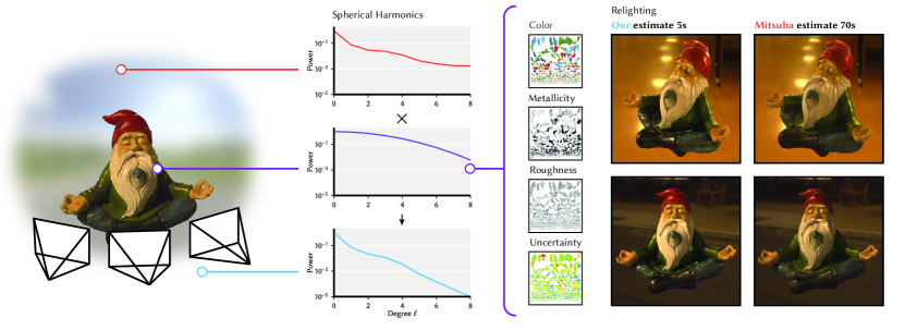
Figure 1. We present fast multi-view material acquisition for objects captured in uncontrolled setups (left). We propose to build upon and extend the signal processing framework for inverse rendering proposed by Ramamoorthi and Hanrahan (2001): we improve the model with shadowing and masking and propose a lightweight objective function for BRDF fitting using spherical harmonics power spectra (center). Using this objective, we propose an uncertainty estimation approach relying on statistical entropy. We show that our material estimation is significantly faster than previous work and achieves similar or better results.

1. Introduction

Object reconstruction is highly attractive for a variety of applications: from creating assets and environments for movies and video games, to preserving cultural-heritage objects digitally. Completely capturing the appearance properties of an object would require hundreds of photographs under controlled viewpoints and lighting conditions. Unfortunately, fine control of the lighting and viewing conditions is inconvenient, and impossible in many setups, such as outdoors or in a crowded museum. In such scenarios only a more “passive” capture of object appearance is possible. In this work, we therefore assume no control over lighting and suppose that views are captured in an unstructured manner. While this type of capture can be enough to recover the geometry of an object, it is more challenging to acquire accurate appearance properties.

Recent approaches for BRDF recovery from (under-constrained) multi-view capture can mainly be classified into two categories: (a) acquisition from only a few images, relying on deep network priors (Deschaintre et al., 2019) and (b) optimizing directly for appearance parameters using differentiable rendering (Jakob et al., 2022; Munkberg et al., 2022). The methods typically do not provide accuracy guarantees, and the latter ones optimize an ill-posed system, without providing any uncertainty measure. The optimization methods are often slow, due to requiring many iterations of full differentiable rendering for every view.

It is easy to miss information about the specular behavior of an object when lighting and viewpoints are uncontrolled, as it requires a lucky alignment of light sources and viewing directions. To shine a metaphorical light on this missing information, we propose to jointly estimate the object’s SVBRDF parameters and the associated uncertainty. We improve upon a seminal work studying inverse rendering problems from a signal-processing perspective in the frequency domain (Ramamoorthi and Hanrahan, 2001). Moving to the frequency domain allows one to gain insight about the expected stability of an inverse rendering system to solve. For example, the incoming light must contain enough amplitude in high-frequency bands to recover certain roughness values for a microfacet BRDF. Otherwise, noise in the signal could make the inversion unstable. Without any amplitude, the inversion would be ill-conditioned, but this is unlikely to occur for natural lighting. Unfortunately, mapping the analysis in the frequency domain to practical algorithms is non-trivial: For instance, samples are often assumed to be equally spaced for frequency analysis while we deal with unstructured sparse samples. Moreover, in its original formulation, the conclusions from Ramamoorthi and Hanrahan (2001) require a priori knowledge of the BRDF to conclude whether the inversion problem is well-conditioned.

In this work, we tackle these problems with an improved frequency-based formulation, providing both computational efficiency and insight into the underlying uncertainty. Our SVBRDF estimation is as accurate as differentiable rendering-based optimization and $13-35$ times faster than the state-of-the-art differentiable path tracer, Mitsuba 3 (Jakob et al., 2022). By finetuning our results with Mitsuba, we achieve better relighting results (+0.5dB PSNR) in less than a third of the time. Thanks to our extension of the signal processing framework, we obtain an accurate estimate of statistical entropy, interpreted as an uncertainty measure for each surface point. We show that this uncertainty can be used to improve acquisition by information sharing or providing information about the information provided by a given view.

To allow meaningful analysis or efficiency gains, we make the assumption that the geometry and lighting are estimated or captured using existing methods. For geometry we can use SDF extraction  (Rosu and Behnke, 2023) or scanning (Kuang et al., 2023), while lighting can be captured using a chrome ball or an omnidirectional camera. This is unlike recent inverse rendering methods, which assume all components are unknown (Munkberg et al., 2022; Sun et al., 2023). Our underlying goal is to make the best use of the available data and to better understand where signal is missing, before resorting to data-driven or ad hoc priors.

Following Ramamoorthi and Hanrahan (2001), we model reflected light from a surface as a convolution of BRDF and incoming light on the hemisphere. To obtain the BRDF, we reconstruct this convolution filter and map it to analytical BRDF parameters. Working in the frequency domain, a convolution is a per-coefficient multiplication, which greatly simplifies analysis and computational complexity. We propose several key improvements to Ramamoorthi and Hanrahan’s approach. First, we handle irregular light-field sampling by transforming the observations of both the outgoing and incoming light into spherical harmonics, using an efficient regularized least-squares approach. Hereby, we can use sparse irregular data from the view sampling as well as regular Fibonacci samples from the environment lighting in a common representation. Next, we include the shadowing and masking terms of the BRDF, discarded by Ramamoorthi and Hanrahan (2001), and update the spherical harmonics coefficients during a parameter gradient-descent optimization. We obtain results on par with a full-featured differentiable rendering system (Jakob et al., 2022). We leverage the relationship between the spherical harmonic power spectra of incoming and outgoing light to define a new objective function for inverse rendering. As this objective is extremely lightweight to evaluate, both in terms of time and memory, we can evaluate the error for many parameter combinations in parallel. We interpret the error as a posterior distribution, encoding how likely each material parameter combination is, given the observations. This statistical perspective lets us compute the entropy of the posterior distribution as a measure of uncertainty. Intuitively, observations that can be well explained by many different parameter combinations lead to a ‘spread-out’ probability distribution with high entropy, which reflects a higher uncertainty. In contrast, when only a few parameter combinations are likely, the distribution is concentrated with low entropy, reflecting high certainty. Similarly, we can estimate the information gain from a new view by estimating its impact on entropy, potentially providing interactive guidance during capture. This uncertainty is also highly relevant to weigh priors, increasing prior weights for uncertain estimations.

We validate our material parameters and uncertainty estimations in both synthetic and real acquisition conditions, comparing the estimation with recent methods. Our solution performs on par with state-of-the-art while being $13$ times faster and providing uncertainty. Further, we validate our refined signal-processing framework through ablation studies, demonstrating clear improvement over Ramamoorthi and Hanrahan (2001). In summary, we enable fast material reconstruction and uncertainty estimation via contributions to the space of SVBRDF estimation from multi-view captures under natural lighting:

• a frequency-space method using spherical-harmonics power spectra for efficient BRDF approximation and parameter exploration from sparse, irregular samples,

• we improve the convolution approximation of Ramamoorthi and Hanrahan by incorporating shadowing and masking,

• we quantify uncertainty in BRDF recovery by leveraging statistical entropy,

• we evaluate various applications for improved reconstruction based on fast acquisition and uncertainty.

We will release our implementation upon acceptance.

2. Related Work

Capturing real-world, spatially varying, surface reflectance models from several camera views has been a long-standing challenge in computer graphics. The operator that maps incoming light from a given direction to outgoing light observed at another direction is a 6D function, the spatially varying bidirectional reflectance distribution function (SVBRDF). Obtaining SVBRDFs from multi-view images has typically been addressed through: optimization, using simplified models, and using data-priors trained on either realistic or synthetic SVBRDFs, or real-world measurements.

2.1. Optimization-based Capture

Various methods recover the associated material properties through optimization using a set of photographs of an object or surface. This task typically requires many photographs and controlled lighting (Aittala et al., 2013; Nam et al., 2018; Dupuy and Jakob, 2018) or object orientations (Dong et al., 2014) during acquisition to guarantee that specular effects are sufficiently observed. Some approaches relied on specialized hardware, for example to capture polarimetric information (Hwang et al., 2022). Others propose to rely on priors, such as stationarity of the captured materials (Aittala et al., 2015, 2016; Xu et al., 2016; Henzler et al., 2021) to compensate for limited information. Multiple methods (Munkberg et al., 2022; Loubet et al., 2019; Nimier-David et al., 2021; Vicini et al., 2022) leveraged the recent progress in differentiable renderings (Nimier-David et al., 2019; Jakob et al., 2022; Nimier-David et al., 2020; Yan et al., 2022; Laine et al., 2020; Nicolet et al., 2023, 2021; Nimier-David et al., 2022; Spielberg et al., 2023; Xu et al., 2023; Wu et al., 2023b; Chang et al., 2023) to propose joint optimization of light, geometry, and material properties. Recent approaches build on novel representations for volumetric scenes, such as neural networks (Mildenhall et al., 2020) and 3D Gaussians (Kerbl et al., 2023), to include optimization for material properties (Boss et al., 2021b, a; Engelhardt et al., 2024; Zhang et al., 2021b; Srinivasan et al., 2021; Jin et al., 2023; Zhang et al., 2021a; Bi et al., 2020; Mao et al., 2023; Zhang et al., 2023; Wu et al., 2023a). In general, these approaches cannot guarantee that the optimized results are accurate, as there is no guarantee that the provided photographs sample the necessary light-view angle pairs to qualify the specular behavior and are unable to provide any measure of certainty. Moreover, they rely on a heavy optimization process. Inspired by Ramamoorthi and Hanrahan (2001) who described BRDFs as multiplications in the frequency domain, we propose to leverage the efficiency of this framework to jointly estimate the material properties and their uncertainty, providing key information about which part of the material properties are likely faithfully reconstructed and for which parts we simply do not have enough information.

2.2. Data priors for Capture

Various approaches propose using data-based priors to simplify and enable low-information acquisition, allowing for estimating (SV)BRDFs from as little as a single image. Many such approaches target flat surfaces, trained on a large amount of data using environmentally lit image(s) (Li et al., 2017; Martin et al., 2022; Vecchio et al., 2023; Shi et al., 2020) or flash-lit image(s) (Deschaintre et al., 2018, 2019, 2020; Shah et al., 2023; Zhou and Kalantari, 2021; Zhou and Khademi Kalantari, 2022; Zhou et al., 2023; Guo et al., 2021) for acquisition. MaterialGAN (Guo et al., 2020) and Gao et al. (2019) propose to optimize in latent spaces of deep neural networks, hereby remaining in the manifold of valid materials. In the context of 3D object acquisition, methods often focus on material extraction using a few (or even single) flash or multi-focal photographs (Li et al., 2018; Deschaintre et al., 2021; Boss et al., 2020; Fan et al., 2023). These approaches are orthogonal to our method, as we focus on recovering the SVBRDF from the provided signal without initial prior, quantifying the uncertainty of the process. Our uncertainty can in turn be used to better guide the use of priors to surface regions which most need it.

2.3. Frequency-based light transport

Our work builds on the frequency analysis of light transport, in particular with the idea that BRDFs can be expressed as low-pass filters (Durand et al., 2005; Ramamoorthi and Hanrahan, 2001). From this, one can express the reflection of light with a BRDF as a multiplication in the frequency domain. This idea has been successfully used in the context of controlled illumination (Ghosh et al., 2007; Aittala et al., 2013), controlling the frequency of light patterns to estimate the BRDF filter parameter through a deconvolution of the reflected light. We do not assume control of the light and operate in the spherical-harmonics frequency domain rather than the Fourier domain ((Aittala et al., 2013)) or custom basis functions ((Ghosh et al., 2007)). This allows our analysis to work with arbitrary natural lighting environments. Closest to our approach is the work by Ramamoorthi and Hanrahan (2001), which explicitly derives the concept of reflection as convolution in a signal-processing framework. They further outline the implications of this perspective on the well-posedness of BRDF- and light estimation from multi-view inputs and optimize for BRDF parameters through the frequency domain. Our work differs in a number of ways: First, we add theoretical insights on uncertainty and sampling. We propose methods to quantify these concepts, so they can be used in downstream tasks and show how to accelerate this approach using the power spectrum. Second, our approach supports arbitrary light setups and treats all frequencies in the same framework, rather than separating high and low frequency lighting. We do so by robustly estimating spherical harmonic coefficients directly on sparse, irregular samples using a regularized least-squares method. Finally, we propose to improve the BRDF model described by Ramamoorthi and Hanrahan to include shadowing and masking and show how to map the model to the widely used simplified principled BRDF (Burley and Studios, 2012).

2.4. Uncertainty estimation

Uncertainty estimation in the context of acquisition is highly desirable, as it can guide the capturing process and the use of priors, or simply inform on the expected quality of a given reconstruction. Lensch et al. (2003a), estimate an object’s material properties by clustering similar BRDF estimations within an object. To guide the clustering and its splitting, the covariance of the parameters are used. In Lensch et al. (2003b), the uncertainty of BRDF parameters is estimated using similar covariance matrices. More recently, Rodriguez-Pardo et al. (2023) taking inspiration from Bayesian methods ((Gal and Ghahramani, 2016)), used Monte-Carlo dropout to estimate the uncertainty of material estimation from a single picture. In the context of novel view synthesis, Goli et al. (2024) propose to evaluate the inherent volumetric uncertainty of NeRF (Mildenhall et al., 2020) reconstructions posterior to training. They use ray perturbations and an approximation of the Hessian to quantify it. They show a correlation between uncertainty and absolute error. In this work, we use a more explicit approach to uncertainty estimation. We use a fast BRDF estimation approximation for many parameter combinations and interpret the resulting error as a negative log-likelihood from which we derive an entropy measure.

3. Background

Our method builds on prior work in inverse rendering and spherical harmonics. We summarize required background knowledge and refer to related work for further depth.

3.1. Spherical Harmonics

Spherical harmonics are a series of orthonormal basis functions on the sphere, indexed by their degree $\ell$ and order $m$. We use them to represent incoming and outgoing radiance over incoming and outgoing directions on the unit sphere. Spherical harmonics are analogous to the Fourier series on a flat domain, where the frequency of the Fourier series corresponds to the degree $\ell$ and order $m$. We provide a brief overview of properties relevant to our method. For further details, a helpful reference and software package is published by Wieczorek and Meschede (2018).

Any real, square-integrable function on the sphere can be expressed as a spherical-harmonics series:

(1) $$f(\theta,\phi)=\sum_{\ell=0}^{\infty}\sum_{m=-\ell}^{\ell}f_{\ell m}Y_{\ell m}(\theta,\phi),$$

where $f_{\ell m}$ is the coefficient for spherical harmonic $Y_{\ell m}(\theta,\phi)$, given as

(2) $$N_{\ell m} =\sqrt{\frac{(2-\delta_{m0})(2\ell+1)}{4\pi}\frac{(\ell-m)!}{(\ell+m)!}}$$

(3) $$Y_{\ell m}(\theta,\phi) =\begin{cases}N_{\ell m}P_{\ell}^{m}(\cos\theta)\cos m\phi&\text{if $m\geq 0$,}\\ N_{\ell m}P_{\ell}^{|m|}(\cos\theta)\sin|m|\phi&\text{if $m<0$.}\end{cases}$$

$N_{\ell m}$ is a normalization factor, $\delta_{m0}$ is the Kronecker delta function, which evaluates to $1$ when $m=0$, and $P_{\ell}^{m}$ is the associated Legendre function for degree $\ell$ and order $m$. The total number of spherical harmonics up to- and including a maximum degree, $\ell^{*}$, equals $(\ell^{*}+1)^{2}$. A useful property of spherical harmonics in our setting is that a rotational convolution on the sphere is equal to multiplication of coefficients in the spherical harmonic domain.

The power spectrum of a spherical function $f$ can be computed from the spherical harmonic coefficients per degree

(4) $$S_{f}(\ell)=\sum_{m=-\ell}^{\ell}f_{\ell m}^{2}.$$

The power spectrum is invariant to rotations of the coordinate system. In our context that means the power spectrum is invariant to slight perturbations of the normals at each point.

3.1.1. Computing spherical harmonic coefficients

One can find the SH coefficients for a function $f$ by computing the inner product with the basis functions

(5) $$f_{\ell m}=\int_{S^{2}}f(\theta,\phi)Y_{\ell m}(\theta,\phi)d\omega.$$

A useful property holds for the coefficient of degree $\ell=0$, for which the spherical harmonic is constant; $Y_{00}(\theta,\phi)=(4\pi)^{-\frac{1}{2}}$. The corresponding coefficient, $f_{00}$, is equal to the integral of $f$ times the normalization constant, $(4\pi)^{-\frac{1}{2}}$. The spherical harmonics for higher degrees all integrate to zero. This is relevant in the context of rendering, because the total integrated incoming and outgoing radiance can be read from the $0^{th}$ degree coefficient and that coefficient alone. In the general case, we estimate the coefficient for $f_{\ell m}$ based on samples of $f$. The sampling method determines how these coefficients are estimated.

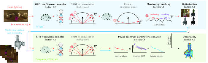
Figure 2. An overview of our pipeline showing input, output, and the proposed algorithm. The input to our approach is a set of photographs of an object from multiple camera points and the associated camera extrinsics and intrinsics. We also provide the input lighting as an environment map and object geometry. Next, we propose two main variants of our approach: a mixed pipeline (top) and a pipeline fully contained in the spherical harmonic domain (bottom). The Mixed pipeline first estimates spherical harmonic coefficients for the input lighting on Fibonacci samples. The light is convolved with the BRDF filter and mapped back to the angular domain, where the outgoing radiance is attenuated with Fresnel, shadowing, and masking. During acquisition, we optimize the BRDF parameters by comparing the outgoing light samples to the radiance captured in the input photographs. The Frequency Domain pipeline first estimates spherical harmonic coefficients on both the incoming and outgoing radiance and then estimates the effect of different BRDF filters within the power spectrum. This is used to compute a measure of uncertainty on the predicted parameters for acquisition.

Regular sampling

If $f$ is sampled on a grid with equally spaced longitudinal and latitudinal angles, this integral can be accelerated using a fast Fourier transform in the longitudinal direction $\phi$ and a quadrature rule in the latitudinal direction $\theta$ (Driscoll and Healy, 1994). In our setting, this approach can be used for environment maps represented as rectangular textures.

Irregular sampling

During capture the camera is often placed at irregular positions, leading to non-uniform $(\theta,\phi)$ samples. Further, a point on the surface might be observed from only a few positions. We therefore often need to use sparse and irregular samples to fit spherical harmonic coefficients. We do so by fitting the coefficients using least-squares, expressing Equation 1 as a linear system

(6) $$\mathbf{Y}\mathbf{c}\approx\mathbf{f},$$

where $\mathbf{f}$ is a vector of $n$ discrete samples from $f$, $\mathbf{Y}$ is a matrix of size $n\times(\ell^{*}+1)^{2}$ containing the spherical harmonics sampled at the same locations as $f$, and $\mathbf{c}$ is a vector of the $(\ell^{*}+1)^{2}$ coefficients we want to find. We can find $\mathbf{c}$ by solving a least-squares system

(7) $$\mathbf{Y}^{\intercal}\mathbf{Y}\mathbf{c}=\mathbf{Y}^{\intercal}\mathbf{f}.$$

To be well posed, this system requires $n>(\ell^{*}+1)^{2}$ independent samples, which can be challenging in the context of sparse sampling, making the system under-constrained. We propose to use a custom regularizer in Section 4.2 for cases where the number of samples is too low.

3.2. Reflection as Convolution

Surface reflection can be approximated as the convolution of incoming radiance (from the light direction) with a BRDF (Ramamoorthi and Hanrahan, 2001). Specifically, if we assume an isotropic microfacet Torrance and Sparrow (1967) BRDF, combined with a Lambertian term, we can derive the following approximate equation for outgoing radiance $B$ at point $p$ in the view direction $\omega_{o}$

(8) $$B(p,\omega_{o})\approx K_{d}E(p)+K_{s}F(\theta_{o})\left[S_{\alpha}\ast L(p)\right]_{\omega_{o}},$$

where $K_{d}$ and $K_{s}$ are diffuse and specular terms; $E(p)$ is the irradiance integrated over the hemisphere; $F(\theta_{o})$ is a simplified Fresnel term, which only depends on the outgoing direction; $L(p)$ is the incoming radiance; and $S_{\alpha}$ is a filter parametrized by the distribution width, $\alpha$. This filter is derived from the normal distribution function of the surface. The $\ast$ operator represents convolution. A derivation of this approximation is included in the Appendix.

In this framework, estimating the specular BRDF parameters comes down to estimating the convolution kernel. This can be done efficiently since a convolution in the angular domain can be represented as a multiplication in the spherical harmonics frequency domain. Using this representation, one can find the convolution kernel through a division of the spherical harmonics coefficients of the outgoing radiance by those of the incoming radiance. This is analogous to kernel estimation for image deblurring in the Fourier domain.

The above leads to crucial insights regarding the well-posedness of BRDF recovery. Ramamoorthi and Hanrahan state that the recovery of BRDF parameters is ill-posed if the input lighting has no amplitude along certain modes of the filter (BRDF). Those modes cannot be estimated without additional priors on plausible spatial parameter variations. For the microfacet BRDF, this leads to the following conclusion: if the incoming light only contains frequencies $\ell<<\alpha^{-1}$, multiplying the coefficients of the light with those of the BRDF only results in a small difference, and the inversion of this operation is ill-conditioned. To accurately estimate $\alpha$, the incoming light used during the capture needs to exhibit sufficiently high frequencies.

This insight is based on a derivation for the coefficients of the microfacet model. The normalized SH-coefficients of the specular component of the BRDF for normal incidence, $S$, are approximated by

(9) $$\hat{f}_{\ell m}\approx e^{-(\alpha\ell)^{2}},$$

which is a Gaussian in the frequency domain with a width determined by $\alpha$. The kernel is derived from a Beckmann normal distribution function and the $\alpha$ parameter corresponds to the $\alpha$ parameter there. Note that these coefficients do not vary with the Spherical Harmonics order $m$, since the normal distribution function is isotropic for outgoing rays in the direction of the normal vector ($\theta_{o}=0$). An important approximation employed by Ramamoorthi and Hanrahan is that this same kernel can be used for any outgoing direction. While the correct kernel varies with the incoming and outgoing direction, this approximation does not lead to significant error for inverse rendering (Ramamoorthi and Hanrahan, 2001) as they note that “it can be shown by Taylor-series expansions and verified numerically, that the corrections to this filter are small [for low degrees $\ell$]”.

In this paper, we expand on the theory established by Ramamoorthi and Hanrahan by improving the reflection as a convolution model’s accuracy and developing the implications for well-posedness into quantifiable metrics on uncertainty without a-priori knowledge on $\alpha$.

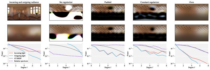
Figure 3. A comparison of the options for fitting spherical harmonics on sparse samples. In the first column, top: incoming radiance (synthetic) on the sphere mapped to a lat-long grid. Middle: synthesized outgoing radiance as a result of filtering incoming radiance with Equation 9, $\alpha=0.2$. Bottom: power spectra of incoming and outgoing radiance and ground-truth filter (BRDF) plotted on a log-scale. In the second to fifth column, we show the result of fitting spherical harmonics coefficients to samples and then transforming back to the spatial domain. We use $100$ samples from the upper hemisphere of the input radiance (first column) and simulate missing samples due to occlusion or missed camera positions by masking some points, leaving $88$ samples. The samples are weighted with $\cos\theta$, which is visualized as the transparency of the samples. We find that our method with a weighted regularizer is able to smoothly interpolate missing values and retrieves the correct BRDF filter in the power spectrum, where other variants overfit, or add dark regions in the upper hemisphere.

4. Method

Our goal is to recover (SV)BRDFs properties and quantify uncertainty from multi-view capture of an object under environment lighting. The input to our method is a set of images $\mathcal{I}$ captured from multiple camera positions. The camera extrinsics, intrinsics, object geometry and HDR lighting are assumed to be known – through existing methods for camera calibration, photogrammetry, and HDR environment capture – but not controlled.

For each point $p$ on the object surface, we know the incoming radiance $L(p,\omega_{i})$ from directions $\omega_{i}$. These values can be sampled from the environment map. For higher accuracy, one can attenuate the light based on self-occlusion, but we do not explore this in our work. By projecting the captured images onto the surface, we retrieve the outgoing radiance at each point, $B(p,\omega_{o})$. Our task is to recover the BRDF $f(p,\omega_{o},\omega_{i})$ and capture the uncertainty associated with its parameters. The BRDF relates the incoming radiance of the upper hemisphere $\Omega$ to the outgoing radiance as (Pharr et al., 2023):

(10) $$B(p,\omega_{o})=\int_{\Omega}f(p,\omega_{o},\omega_{i})L(p,\omega_{i})\cos\theta_{i}d\omega_{i}.$$

We use the  Torrance and Sparrow (1967) BRDF model with parameters for diffuse reflectance $K_{d}$, specular reflectance $K_{s}$, and the slope of the normal distribution function $\alpha$ (Equation 8). We denote these parameters as a vector of parameters, $\psi$. In subsection 4.6, we show how to map a simplified Disney principled BRDF (Burley and Studios, 2012) to these parameters.

To estimate $\psi$, we propose to build on the framework proposed by Ramamoorthi and Hanrahan (2001). In the following sections we carefully highlight how we improve and extend its use compared to the original formulation. An overview of the pipeline is shown in Figure 2, where we denote our contributions in black and existing work in gray. In particular, we describe the extension of the existing convolution model to take shadowing and masking effects into account. We then describe an efficient spherical-harmonics fitting from sparse and irregular samples of radiance, enabling unstructured capture setups. We then propose a carefully validated approximation of the convolution model to design a lightweight loss function, leveraging the power spectrum for efficient loss evaluation. These improvements enable quick sampling of the BRDF parameter space, $\Psi$, which we use to propose a new formulation for capturing uncertainty relying on statistical entropy. Finally, we map the Torrance-Sparrow BRDF model parameters to those of the simplified Disney principled BRDF (Burley and Studios, 2012) for use in modern rendering pipelines.

4.1. Improving the Convolution Model

The approximate reflection function in Equation 8 does not include the shadowing or masking terms present in microfacet models (Pharr et al., 2023). The shadowing and masking terms model occlusion on incoming light (shadowing) and outgoing light (masking) due to the configuration of the microfacets (Figure 2, top right). Light at grazing angles is more likely to be occluded by microfacets, especially if the microfacet distribution is wide (high roughness). Ramamoorthi and Hanrahan argue that these terms can be ignored, because they mostly affect observations made at grazing angles. While this is true for materials with low roughness, we find that ignoring this term leads to reconstruction errors for high roughness materials – we evaluate the terms’ impact in Table 4. We therefore propose to introduce shadowing and masking terms to the convolution model.

Shadowing and masking effects are typically modeled jointly to avoid an over-correction of the radiance (Pharr et al. (2023), Section 9.6.3). However, this joint term cannot be included in the simplified convolution model as presented in Equation 8, because the kernel would need to vary with both $\omega_{i}$ and $\omega_{o}$ (the 2D kernel only varies with either $\omega_{i}$ or $\omega_{o}$). Therefore, we assume that shadowing and masking effects are independent and can be modeled separately as $G_{\alpha}(\omega_{i})G_{\alpha}(\omega_{o})$. While we do observe a small overestimation of the shadowing and masking effect, we show in Table 4 that the addition of the term still leads to improvements for BRDF acquisition. This way we can first attenuate the incoming light with the shadowing term, then convolve with the BRDF and then attenuate the result with the masking term

(11) $$B(p,\omega_{o})\approx K_{d}E(p)+K_{s}F(\theta_{o})G_{\alpha}(\theta_{o})\left[S_{\alpha}\ast G_{\alpha}(\theta_{i})L(p)\right]_{\omega_{o}},$$

where $G_{\alpha}$ is the shadowing-masking function in the Trowbridge and Reitz (1975) model (also referred to as GGX (Walter et al., 2007)). The shadowing and masking terms both depend on $\alpha$, which is not known a-priori. This means that the shadowing and masking terms change as we optimize $\alpha$. As a consequence, we need to update the coefficients for the incoming light as $G_{\alpha}(\theta_{i})$ changes. While the estimation of spherical harmonic coefficients is relatively fast, it can still be quite cumbersome to update the coefficients in every optimization step. Therefore, we only update the shadowing term each $m$ iterations.

4.2. Fitting Spherical Harmonic Coefficients

Much of our computation relies on a convolution applied in the spherical harmonics domain, which means we require a good spherical harmonics transform. This is challenging, because the outgoing light field, $B$, is sampled sparsely and non-uniformly (Figure 3, second column). Therefore, Ramamoorthi and Hanrahan do not directly estimate spherical harmonic coefficients on $B$, but only perform the transformation from the spherical harmonic domain to the directional domain. This is simpler, because it only requires evaluating the spherical harmonics at the sample locations (Equation 1). For the incoming light, they represent low-frequency (area sources) and high-frequency lighting (point sources) separately and limit their environments to controlled ‘lightbox’-like settings. We would like to compute an estimate of the spherical harmonic coefficients for the outgoing radiance, because this would enable algorithmic analysis fully within the frequency domain. This is highly appealing, because it has the potential to greatly simplify the analysis of BRDF recovery, as showcased by Ramamoorthi and Hanrahan (2001).

Next to sparse sampling, a significant challenge is that both the incoming- and outgoing radiance fields are only supported on the upper hemisphere when considering reflection. If we were to consider incoming radiance on the lower hemisphere, we would implicitly model light ‘leaking through’ the surface. One possible solution is to simply pad the lower hemisphere with zeros (Figure 3, third column). This is not practical, because it introduces high frequency variation at the boundary, which disrupts any potential analysis on the spherical harmonic coefficients (bottom row). Another solution that we explored is to represent the radiance fields with hemispherical harmonics (Zheng et al., 2019). In practice, this is equivalent to mirroring the radiance fields along the meridian, which resulted in mismatches with the convolution model.

We instead propose a spherical harmonics fitting approach that is robust to sparse and irregular samples, and supports the lack of lower hemisphere samples and gracefully handles occluded regions. First, analog to ideas from compressed sensing, we add a regularization term on the spherical harmonic coefficients. A typical choice for this term is an $L1$ norm, which enforces sparsity in the spherical harmonic coefficients. The resulting system can be solved with linear programming. We propose instead to use a weighted $L2$ norm which can be solved using standard linear solvers, which we found to be faster and more stable for our usecase:

(12) $$(\mathbf{Y}^{\intercal}\mathbf{Y}+\lambda\mathbf{W})\mathbf{c}=\mathbf{Y}^{\intercal}\mathbf{f},$$

where $\mathbf{W}$ is a diagonal weight matrix. If constant, this weight matrix leads to poor fitting as the regularization is too strong on the lower spherical harmonics degrees (Figure 3, fourth column). We set the weight equal to $e^{\ell}$, increasing the strength of regularization for higher spherical harmonics degrees. This is informed by the observation that many natural images have a power spectrum with exponential decay (Fleming et al., 2003). Intuitively, this regularizer encourages filling unknown regions with low-frequency information, akin to solutions with a smoothness term (Figure 3, right-most column). By applying the same regularization to both incoming- and outgoing radiance fitting, we are able to recover the correct filter (bottom row), even though the recovered incoming radiance looks blurrier (top row).

We fit the signals for which we have complete spatial information (e.g., incoming environment light) by sampling it in with Fibonacci samples on the sphere. For partially observed signal (e.g., reflected light) we use the available samples with the described fitting technique for sparse and irregular samples. An important consideration related to the number of samples, is the frequency of the signal that we fit spherical harmonics to. We have an in-depth analysis of this in the Appendix. The practical take-away is that the incoming signal should be bandlimited to roughly $n^{\frac{1}{2}}$ to avoid aliasing, where $n$ is the number of input views. We ensure this is the case for the incoming radiance by applying the filter in Equation 9 with $\alpha^{\prime}=n^{-\frac{1}{2}}$ on the input environment map. The impact on our BRDF estimation is that we cannot accurately recover $\alpha<\alpha^{\prime}$. In our experiments and analysis in the Appendix, we find that the recovered $\alpha$ tends to be between $0$ and $\alpha^{\prime}$ in those cases. A second finetuning pass with a differentiable path tracer, like the one we demonstrate in the experiments, can help refine those regions.

4.3. Optimizing for SVBRDF Parameters

Using our more complete model described in Equation 11, we can optimize for the object’s material parameters using gradient descent:

(13) $$\psi^{*}=\arg\min_{\psi}\sum_{p,\omega_{o}}|B_{\psi}(p,\omega_{o})-B^{\prime}(p,\omega_{o})|$$

With $B_{\psi}(p,\omega_{o})$ a rendering operator using Equation 11 and $B^{\prime}$ the radiance values projected onto the surface points $p$. As described in subsection 4.1, we optimize the parameters $\psi$ for a number of iterations before updating the shadowing term, as this step requires recomputing the spherical harmonic fit. The masking term is included in the forward rendering step and updated every iteration. Because of the simplicity of the convolution approximation, we are able to optimize for all points and camera positions in one go, rather than using stochastic gradient descent with batches of rays. This lets us run our optimization with fewer iterations than other approaches. Similar to other methods, we add the total variation norm on the parameters in texture space as a regularizer to enforce smoothness, weighted with $1\text{\times}{10}^{-3}$.

4.4. A Lightweight Objective

In this section we define a particularly efficient-to-compute approximation of the convolution BRDF model described in Equation 11. Our goal is to develop algorithms to analyze the inverse rendering problem fully in the spherical harmonic domain. This would simplify such analysis tremendously, as convolution is simply a per-frequency multiplication in this domain.

For this approximation, we propose to ignore the Fresnel and shadowing and masking terms, letting us express the reflection function entirely in terms of spherical harmonic coefficients. We show experimentally in Section 5.4.2 that the impact of this approximation is acceptable on the underlying application of this objective. Using Equation 9 for the coefficients of $S$ we get:

(14) $$B_{\ell m}=\begin{cases}{\pi}^{-\frac{1}{2}}K_{d}E(p)+K_{s}L_{\ell m},&\text{if $\ell=0$}.\\ K_{s}e^{-(\alpha\ell)^{2}}L_{\ell m},&\text{otherwise}.\end{cases}$$

We note that the specular component for $\ell=0$ does not depend on $\alpha$, because for $\ell=0$, Equation 9 equals $1$. The term ${\pi}^{-\frac{1}{2}}K_{d}E(p)$ represents the diffuse component as a constant function. We know, based on the conservation of energy, that the diffuse component should integrate to $K_{d}E(p)$ on the upper hemisphere for outgoing directions. Thus, the integral over the full sphere should be $K_{d}2E(p)$. Equation 5 shows that the Spherical Harmonics coefficient for degree $\ell=0$ should be equal to $(4\pi)^{-\frac{1}{2}}$ times the integral: $(4\pi)^{-\frac{1}{2}}K_{d}2E(p)={\pi}^{-\frac{1}{2}}K_{d}E(p)$. From this expression, we make two observations. (a) We cannot recover the ratio between $K_{d}$ and $K_{s}$ from the $\ell=0$ alone, as we have two unknowns and only one coefficient and (b) we cannot derive any information on $\alpha$ from the 0th degree, as it has no impact there. It follows that we can only recover $K_{s}$ and $\alpha$ from degrees $\ell>0$. Once $K_{s}$ is known, we can then estimate $K_{d}$ from the 0^th degree. In other words, we know diffuse reflectance once we know the contribution of the specular component. This reduces our analysis of uncertainty to the specular component on the parameters $K_{s}$ and $\alpha$. Note that this simplification comes naturally in the frequency domain, because we can limit our analysis to degrees $\ell>0$. This is non-trivial to separate out in the directional domain.

We use our proposed spherical harmonic coefficient fitting described in Section 4.2 to recover $L_{\ell m}$ and $B_{\ell m}$. $B_{\ell m}$ is estimated from the sparse, irregular samples of the object from the input views as described in Section 4.2. $L_{\ell m}$ is estimated from samples of the environment in the reflection directions of the viewing positions. This ensures that the spherical harmonic coefficients for $L$ and $B$ are comparable and that we can analyze the frequencies of the observed light.

Next, we propose to use the power spectra $S_{L}$ and $S_{B}$ of the spherical harmonics fittings $L_{\ell m}$ and $B_{\ell m}$, which we can express as

(15) $$S_{L}(\ell) =\sum_{m=-\ell}^{\ell}L_{\ell m}^{2}$$

(16) $$S_{B}(\ell) =\sum_{m=-\ell}^{\ell}(K_{s}e^{-(\alpha\ell)^{2}}L_{\ell m})^{2}$$

(17) $$=K_{s}^{2}e^{-2(\alpha\ell)^{2}}\sum_{m=-\ell}^{\ell}L_{\ell m}^{2}$$

(18) $$=K_{s}^{2}e^{-2(\alpha\ell)^{2}}S_{L}(\ell)$$

for degrees $\ell>0$. Using this relationship between the BRDF parameters ($K_{s}$, $\alpha$) and the incoming and outgoing radiance power spectra ($S_{L}(\ell)$ and $S_{B}(\ell)$, we can formulate a lightweight objective:

(19) $$D(K_{s},\alpha)=\sum_{\ell=1}^{\ell^{*}}(S_{B}(\ell)-K_{s}^{2}e^{-2(\alpha\ell)^{2}}S_{L}(\ell))^{2}.$$

Intuitively this objective evaluates the difference between the observed radiance and the BRDF-convolved incoming radiance with a given ($K_{s}$, $\alpha$) through their respective power spectrum. This formulation reduces the computation from $\ell^{*2}$ to $\ell^{*}$ evaluations of the objective, making its evaluation near instantaneous. We show how this fast estimation is key to unlocking near-instant (¡1ms) uncertainty evaluation as shown in Section 4.5 and can be used as initialization of the optimization described in Section 5.6.

4.5. Entropy as Uncertainty

In our context of passive acquisition, we have no guarantee that the illumination on the captured object surface is sufficient to fully recover the material parameters. This uncertainty is particularly desirable information as it is key to understanding the quality of acquisition (e.g. for digital twins), driving the use of priors in uncertain regions while preserving the correctly recovered surface areas, or driving the acquisition by maximizing the information provided by new views when additional captures are possible. We propose to use a grid search of the parameter space to inform our uncertainty estimation. This is now tractable, thanks to the power spectrum approximation discussed in the previous section. By interpreting the error over the parameter space as a likelihood function, we can express uncertainty using entropy, which is a common way to study uncertainty. We detail these contributions in the following paragraphs.

One can interpret the recovery of the right BRDF parameters, $\psi^{*}$ as a maximization of the posterior probability distribution of the parameters given the incoming and outgoing power spectrum

(20) $$\psi^{*}=\arg\max_{\psi}\,p(\psi|S_{L},S_{B}).$$

According to Bayes rule, the posterior is proportional to the product of the likelihood and prior over the parameters:

(21) $$p(\psi|S_{L},S_{B})\propto\mathcal{L}(S_{L},S_{B}|\psi)q(\psi),$$

Assuming $q(\psi)$ to be an uninformative prior, i.e. a uniform distribution on the range of allowed parameter values (typically [0,1] for BRDF parameters), we can reformulate this objective to an equivalent negative log-likelihood objective

(22) $$\psi^{*}=\arg\min_{\psi}-\log(\mathcal{L}(S_{L},S_{B}|\psi)).$$

We interpret the lightweight objective described in Equation 19 as the Negative Log Likelihood (NLL) of the joint probability, given parameters $\psi=(K_{s},\alpha)$:

(23) $$\mathcal{L}(S_{L},S_{B}|\psi)=\frac{1}{\sigma\sqrt{2\pi}}e^{-\frac{1}{2\sigma^{2}}D(K_{s},\alpha)},$$

where $D(K_{s},\alpha)$ is the squared error measure defined in Equation 19. We can view this as assuming that the error of our model caused by approximations and measure noise is Gaussian $\sim\mathcal{N}(0,\sigma^{2})$. We set $\sigma=1e^{-2}$, found empirically to capture the change in loss observed when noticeably changing $\psi$. The scaling constant above is optional since we will renormalize below in Equation 24. With $\sigma$ fixed, minimizing the NLL from Equation 22 is equivalent to minimizing $D(K_{s},\alpha)$.

We explore the material parameter space for $\psi=(K_{s},\alpha)$, discretized in $n$ values in total, $\psi_{i=0..n}$ ($\sqrt{n}$ per variable). Because this process can be parallelized easily, this step typically takes between $1-10$ms for common scenarios. The grid search provides us with a discrete distribution $d$ obtained from the $n$ samples of $\psi$:

(24) $$d_{i}=\frac{\mathcal{L}(S_{L},S_{B}|\psi_{i})}{\sum_{i=1}^{n}\mathcal{L}(S_{L},S_{B}|\psi_{i})},$$

where $d_{i}$ gives the probability that a parameter is within a range of $1/2n$ from $\psi_{i}$. We use the discrete distribution to compute the uncertainty with the distribution’s normalized entropy:

(25) $$H=-\frac{1}{\log(n)}\sum_{i=1}^{n}d_{i}\log(d_{i}).$$

Intuitively, the normalized entropy describes the spread of a probability distribution: low entropy means that the probability distribution is highly concentrated, which implies certainty. High entropy means that the probability distribution is spread out, which implies uncertainty: many options share a similarly high probability.

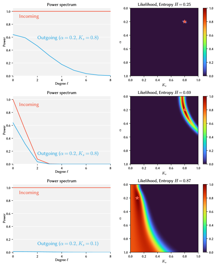
Figure 4. Examples of the likelihood and entropy $H$ resulting from three sets of power spectra for incoming and outgoing radiance. The likelihood is sampled at $100$ discrete values. Top: An ideal situation, where the incoming radiance is a dirac delta (all frequencies are present). Middle: A situation where the incoming radiance does not have enough amplitude for higher degrees. Bottom: A situation where the incoming radiance is ideal, but the specular component is too low to get a proper recovery for $\alpha$.

We show three examples of power spectra, their corresponding likelihood and entropy in Figure 4. The top row shows incoming light for a dirac delta light source (constant in the spherical harmonic domain) and we see that entropy is low ($H=0.25$) and that it is simple to recover the correct parameters. The middle and bottom rows are problematic cases. In the middle row, the light only has amplitude in low frequencies and many roughness values are equally likely ($H=0.69$), in line with the conclusions from Ramamoorthi and Hanrahan. The bottom row shows a material with very low specular reflectance, resulting in high entropy ($H=0.87$). This could result in incorrect estimates under noisy conditions. Concluding, entropy as uncertainty generalizes and quantifies the observations made by Ramamoorthi and Hanrahan on the uncertainty for certain incoming light and material parameters, without requiring a prior estimate of the BRDF parameters.

4.6. Disney Principled BRDF

Many modern rendering pipelines employ variants of the Disney BRDF (Burley and Studios, 2012), which is a combination of a diffuse term and a microfacet term with a user-friendly parametrization. The model also contains some additional features beyond the scope of the current work. We can formulate our model using the principled BRDF parameters, rather than the raw parameters of the Torrance-Sparrow model. We parameterize base color, metallicity and roughness, mapping these to the Torrance-Sparrow model as

(26) $$K_{d} =R_{b},$$

(27) $$K_{s} =1,$$

(28) $$R_{0} =0.04+(R_{b}-0.04)m,$$

(29) $$F(\theta_{o}) =R_{0}+(1-R_{0})(1-\cos\theta_{o})^{5},$$

(30) $$\alpha =r^{2},$$

where $R_{b}$ is the base color, $m$ is the metallicity parameter and $r$ is the roughness. In the ablations where the Fresnel term is not used, we set $K_{s}=R_{0}$. Note that we set $K_{s}$ to $1$, because the specular term is contained in the Fresnel term as $R_{0}$.

	Base Color	Roughness	Metallic	Entropy	Relighting 1	Relighting 2	Relighting 3	Relighting 4
Ours
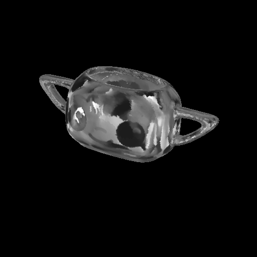
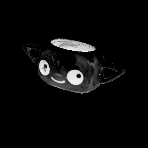
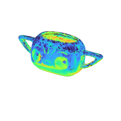
Mitsuba
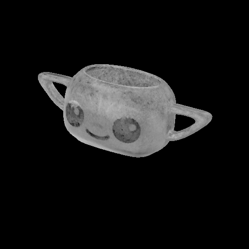
Photographs	Inputs
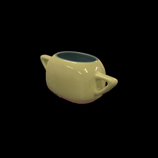
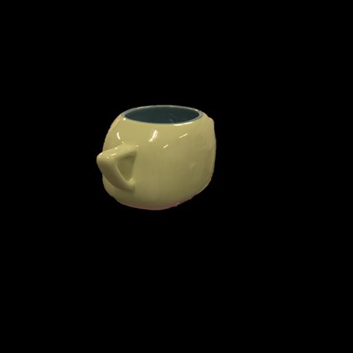
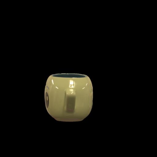
Ours
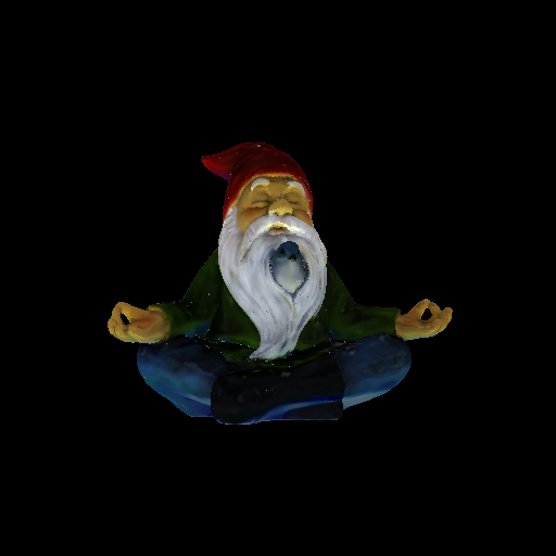
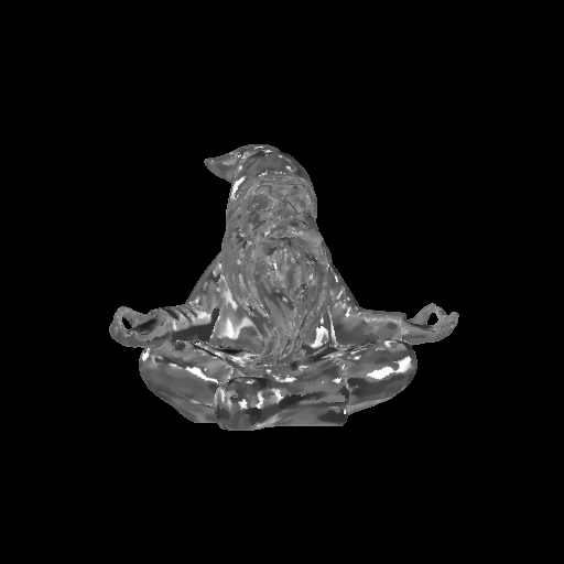
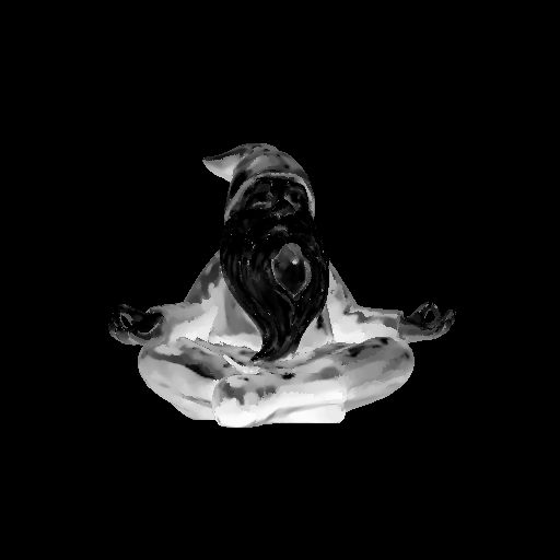
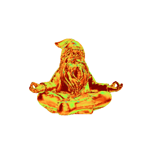
Mitsuba
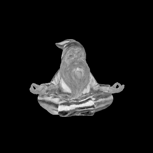
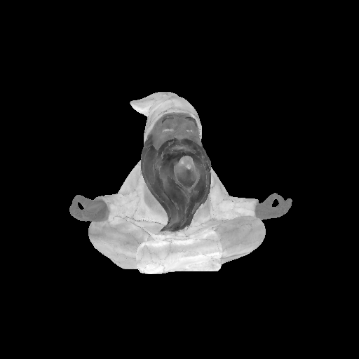
Photographs	Inputs
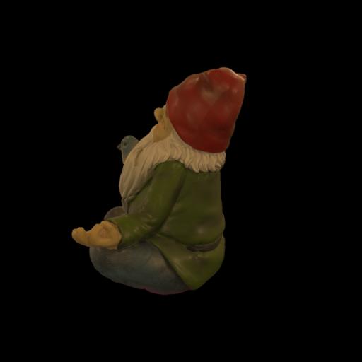
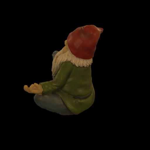
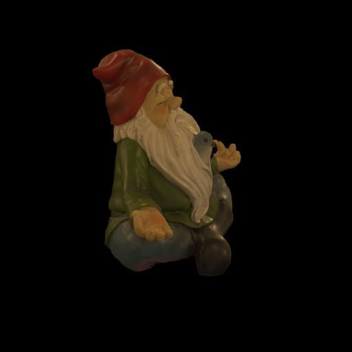
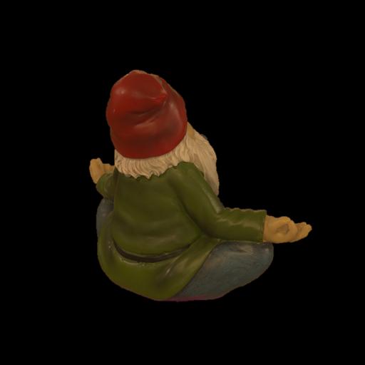
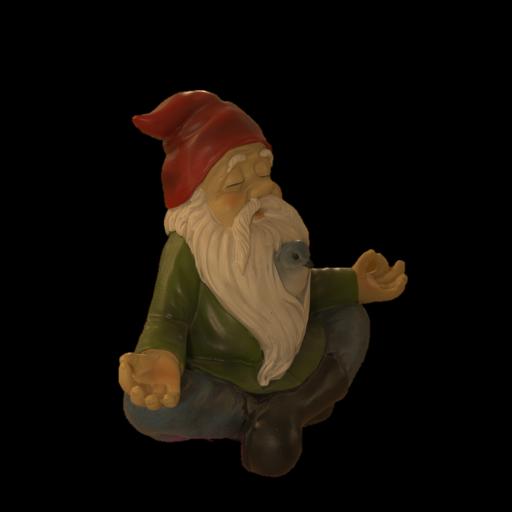
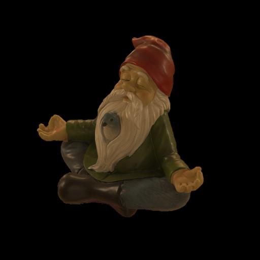
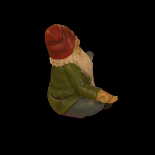
Ours
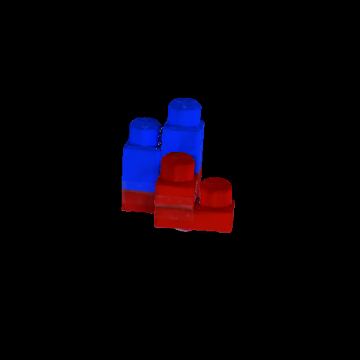
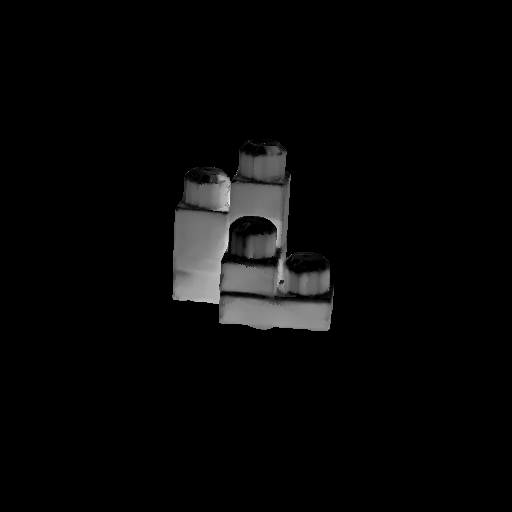
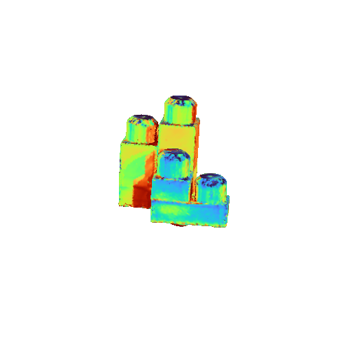
Mitsuba
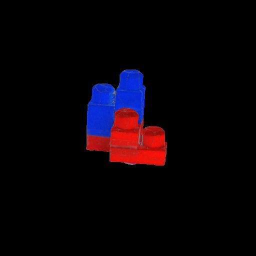
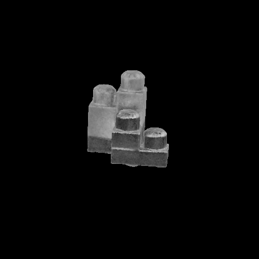
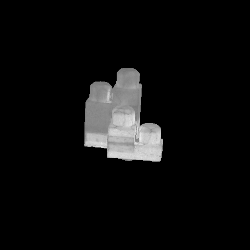
Photographs	Inputs

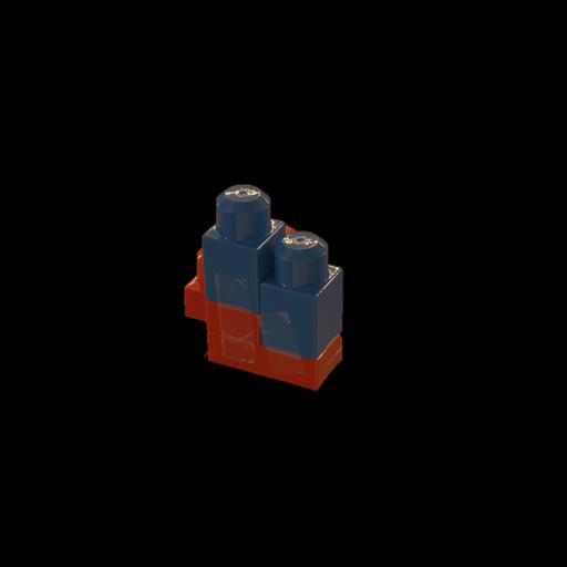
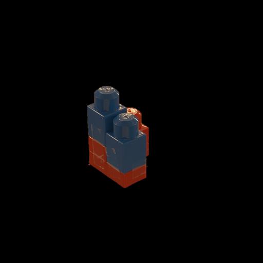
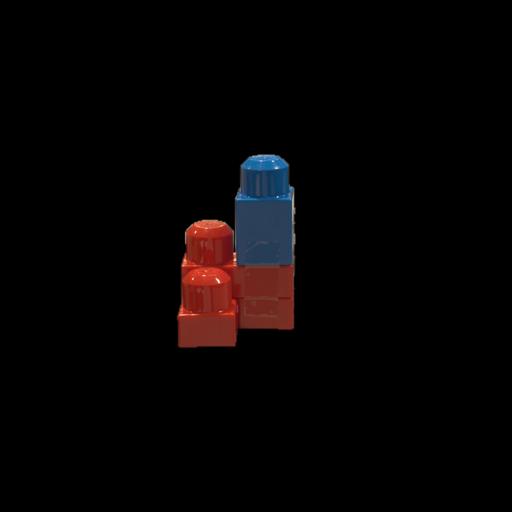
Figure 5. We compare our approach to Mitsuba and photographs for relighting. The first column on the left shows material parameters and training photographs, while the right column shows relit results and photographs under different lighting. We see that our results match the appearance of the photographs as well- or slightly better than Mitsuba. We see that the entropy is lower where inputs provide more information (e.g. well-lit regions). Videos in the Supplement.

5. Experiments

Our method yields two main benefits: fast fitting and a measure of uncertainty. In our experiments, we validate these benefits with comparisons, provide insight into variations of the algorithm in ablations, and show applications to demonstrate potential use cases.

5.1. Implementation

We implement our full pipeline in PyTorch. The output of our method is a set of PBR textures (roughness, metallicity, base color) which are mapped to the input mesh with UV-coordinates to 512x512 textures. For re-renders, we feed the textures produced by our method into Mitsuba, which is possible due to the mapping to the principled BRDF described in subsection 4.6. Each timing result is reported on a machine with an NVIDIA RTX4090 GPU and an AMD Ryzen 9 7950X 16-Core CPU. We will publish the code for our experiments with scripts to replicate each table upon publication.

Our main comparison target is Mitsuba 3 (Jakob et al., 2022), as it is a well-documented, open-source, and research-friendly package for differentiable rendering. More recently Sun et al. (2023) propose to jointly optimize for lighting, material and geometry, but did not yet release a public implementation; given that they rely on a complex differentiable renderer, we believe Mitsuba 3 to be the best proxy for their inverse PBR step. When optimizing with Mitsuba, we sample one ray per pixel in each view. The material parameters are optimized with stochastic gradient descent, where the gradient for each step is estimated with a random set of rays to ensure good convergence. Each primary ray is sampled $32$ times, allowing the reflection directions to be sampled. We run an Adam optimizer until convergence or a maximum of $10$ epochs.

5.2. Datasets

We perform experiments on a recent in-the-wild benchmark dataset, Stanford ORB (Kuang et al., 2023) and on synthetic scenes. Stanford ORB contains $14$ objects, each captured $3$ times in different scenes (lighting environments), selected from a total of $7$ scenes. The lighting environment is captured through a chrome ball and stored as a lat-long environment map. Each object is also scanned in a separate stage, providing high-quality geometry. For our evaluation, we focus on the (SV)BRDF recovery step and use the provided geometry. In our experiments, we optimize material parameters for each object, for each of the three environments, and test against the photographs of the same object in the two environments that were not observed during optimization.

For the synthetic benchmark, we selected $15$ objects with spatially varying BRDF textures for base color, roughness and metallicity. We selected four environment maps with varying challenges to render the objects: two indoor scenes, one outdoor scene with a clear sky and sun, and one overcast outdoor scene. Because we have ground-truth material textures for the synthetic scenes, we can quantitatively evaluate our optimization results and validate uncertainty directly on the optimized parameters. The objects are rendered in Mitsuba at $512\times 512$ resolution and $256$ samples per pixel. Renders and ground truth views for both Stanford ORB and the synthetic benchmark are included in the Supplement.

5.3. Acquisition comparison

We validate that our improved convolution model results in high-quality acquisition results. We also quantify the benefit of our method compared to other methods regarding optimization time. We test our approach on Stanford ORB and synthetic scenes.

5.3.1. Stanford ORB

The similarity metrics for relighting results on Stanford ORB are presented in Table 1. We find that our approach performs on par with Mitsuba, while demonstrating a 13 times speedup with little optimization on our side (e.g., we do not implement custom CUDA kernels and use pure PyTorch). We also compare to NVDiffRec, as it leverages a differentiable rasterizer, and show that our method achieves better relighting results. For NVDiffRec, given that we optimize for materials only, we monitor the loss and record the time for good convergence. We empirically find 2000 steps to be sufficient for this dataset. We qualitatively compare our results to Mitsuba and photographs of the objects under the same illumination in Figure 5 and against NVDiffRec in supplemental material. We present a view of our material channels projected on the captured object and a few input photographs. The entropy is visualized using the ”Turbo” colormap. On the four right columns, we present renderings of our results and Mitsuba under a novel illumination and compare them against photographs of the object taken under that same illumination. We can see that our approach recovers similar appearance in a fraction of the time.

5.3.2. Synthetic

	Base Color	Roughness	Metallic	Entropy	Relighting 1	Relighting 2	Relighting 3
Ours
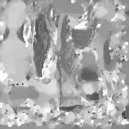
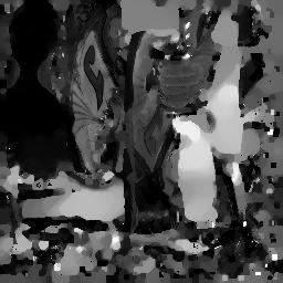
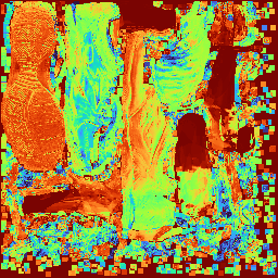
Mitsuba
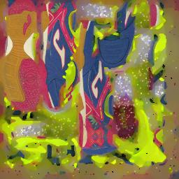
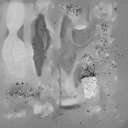
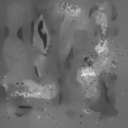
Ground Truth
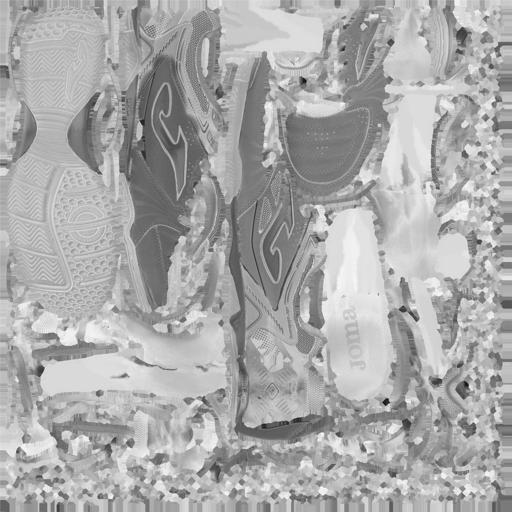
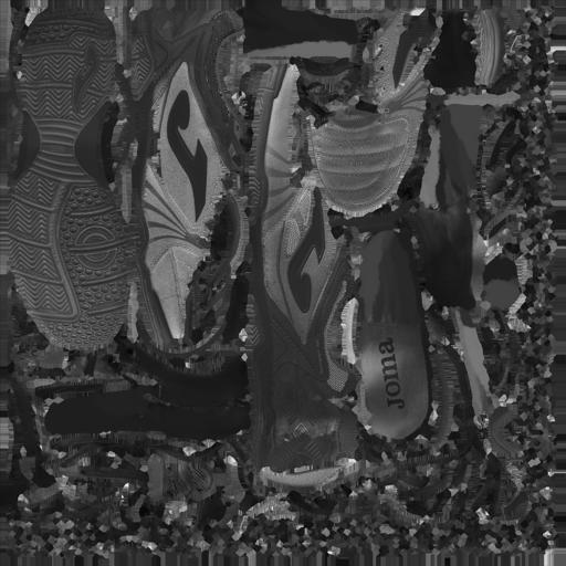
Ours
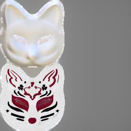
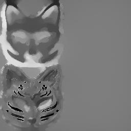
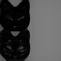
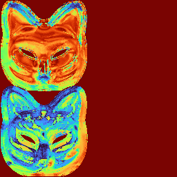
Mitsuba
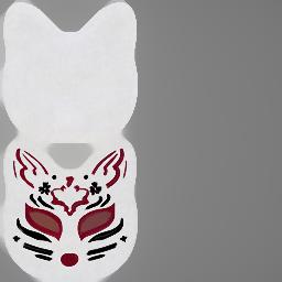
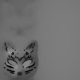
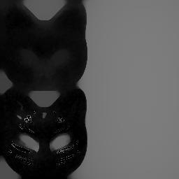
Ground Truth
Ours
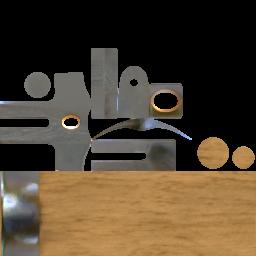
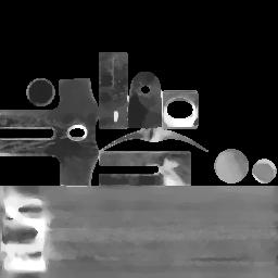
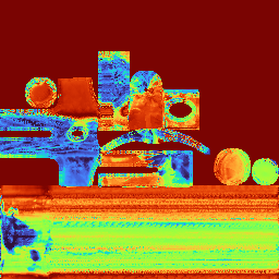
Mitsuba
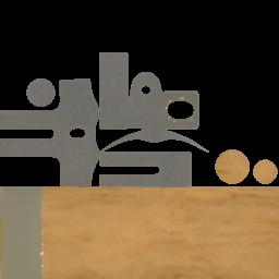
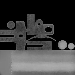
Ground Truth

Figure 7. We compare our results to Mitsuba and ground truth parameters on synthetic data. We see that we achieve similar matching quality with a $35$x speedup in the optimization. The relit renderings are from test views using a lighting environment unseen during optimization. Here too we see that entropy is higher where inputs provide less information (see supplemental materials for inputs).

For synthetic datasets, we compare the recovered material parameters with the ground-truth parameters. We show the results in Table 2, demonstrating comparable accuracy compared to Mitsuba despite particularly challenging objects for our method (e.g. with significant inter-reflections – metallic chess pieces and self-occlusion – donut). We also show a qualitative evaluation in Figure 7, showing the parameters in UV space alongside the entropy maps (visualized using the “Turbo” colormap) for results optimized from images rendered under the “rural asphalt road” environment light. On the right columns we compare rerenderings of our results and Mitsuba’s to ground-truth renderings under a different illumination, showing once more a good appearance match. We include visual comparisons on all synthetic cases as well as the exr files for all light environments in Supplemental Material.

Table 1. Benchmark Comparison for Novel Scene Relighting from (Kuang et al., 2023). All the models listed in this table were trained with the ground-truth 3D scan and ground-truth, in-the-wild environment maps. We report evaluations on the same dataset and task under different acquisition conditions in the Appendix.

	PSNR-H$\uparrow$	PSNR-L$\uparrow$	SSIM$\uparrow$	LPIPS$\downarrow$	Time
NVDiffRec (Munkberg et al., 2022)	24.319	31.492	0.969	0.036	142.143s
Mitsuba (Jakob et al., 2022)	$26.595$	$\mathbf{34.185}$	$\mathbf{0.977}$	$0.032$	$69.96$s
Ours	$\mathbf{26.677}$	$33.936$	$\mathbf{0.977}$	$\mathbf{0.029}$	$5.27$s
Ours - Spectrum Only	$24.478$	$31.117$	$0.971$	$0.037$	$\mathbf{1.96}$s
Ours + Mitsuba (1 epoch)	$27.038$	$34.560$	$\mathbf{0.978}$	$0.030$	$19.87$s
Ours + Mitsuba (2 epochs)	$\mathbf{27.199}$	$\mathbf{34.770}$	$\mathbf{0.978}$	$\mathbf{0.029}$	$33.39$s

Table 2. Synthetic benchmark comparison (MSE) of Mitsuba and our method to the ground-truth parameters. For each environment we present the error in the following way: Average (Base Color, Roughness, Metallicity). We also report for each environment the correlation between the entropy we compute with our power spectrum approximation and the error in Mitsuba’s optimization to show that our entropy is useful for general inverse rendering pipelines.

	Photo Studio	Overcast	Museum	Rural Road	Avg.	Time
Mitsuba	$0.04$ ($0.01$, $0.03$, $0.07$)	$0.03$ ($0.01$, $0.02$, $0.06$)	$0.04$ ($0.01$, $0.04$, $0.08$)	$0.04$ ($0.01$, $0.03$, $0.07$)	$0.04$ ($0.01$, $0.03$, $0.07$)	$105.19$s
Ours	$0.07$ ($0.02$, $0.09$, $0.10$)	$0.06$ ($0.02$, $0.07$, $0.09$)	$0.07$ ($0.02$, $0.08$, $0.11$)	$0.05$ ($0.01$, $0.05$, $0.08$)	$0.06$ ($0.02$, $0.07$, $0.09$)	$3.14$s
Ours - Spectrum Only	$0.19$ ($0.07$, $0.15$, $0.37$)	$0.20$ ($0.06$, $0.14$, $0.40$)	$0.25$ ($0.09$, $0.20$, $0.46$)	$0.22$ ($0.06$, $0.16$, $0.43$)	$0.21$ ($0.07$, $0.16$, $0.41$)	1.20s
Error-Entropy correlation	$0.21$	$0.13$	$0.18$	$0.14$	$0.16$	-

5.4. Uncertainty

We test whether our proposed entropy-based uncertainty metric is indicative of error in inverse rendering results and representative for uncertainty in other inverse rendering frameworks.

5.4.1. Stanford ORB

Our first claim is that the entropy computed using our power spectrum or other differentiable renderers will be similar. We validate this by computing our proposed entropy on the Stanford ORB dataset with Mitsuba, on a grid of $8\times 8\times 8$ parameters (roughness, metallicity, base color). We compute the Pearson correlation coefficient, $\rho$, between entropy computed with our power spectrum approximation and the one computed with Mitsuba’s fully-fledged differentiable renderer. We find a high correlation between entropy computed with Mitsuba and both our mixed renderer $\rho=0.90$ and the power spectrum approximation $\rho=0.89$ as shown in Table 3. This validates that the entropy we compute with our power spectrum based model is indeed similar to that computed with a fully-fledged differentiable renderer. Further, as our power spectrum approximation is embarrassingly parallelizable, we obtain extreme speedups over both the mixed spherical harmonics method ($2645\times$) and Mitsuba ($800,000\times$) making our uncertainty estimation very practical.

5.4.2. Synthetic dataset

We also evaluate whether low entropy is associated with lower error after optimization, even for results optimized with another approach (Mitsuba), indicating if enough information is in the input. If entropy is high, we have a higher likelihood of incorrect parameters, though they might still be good. Indeed we do not expect a one-to-one correlation ($\rho=1$). For example, if the likelihood for parameters in uncertain regions is uniform, low error in a high entropy part is equally likely as high error. That means a correlation of $0.5$ is the most we can reasonably expect. We study this by computing the correlation between entropy computed using the power spectrum approximation and the squared error between the ground-truth material parameters and the parameters optimized with Mitsuba. On top of uncertainty, there could be other factors for error, which could result in lower correlation (such as global illumination approximations, approximate light environment, and incorrect geometry). In the last row of Table 2 we show the correlation scores. We show in Figure 6 results optimized from images rendered under the lighting environment “rural asphalt road” which presents a strong directional illumination (sun, outdoor, see supplemental folder). We can see that areas which are not directly lit by the sun in the input images exhibit higher entropy, intuitively, without enough observed specular signal, uncertainty is high (this is particularly visible on the dice example in the synthetic Supplemental Materials where 3 faces are well lit, and their opposed faces are not).

One Input View	GT Base Color	Estimated Base Color	GT Roughness	Estimated Roughness	GT Metallicity	Estimated Metallicity	Estimation Error	Our Entropy

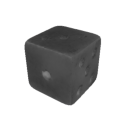
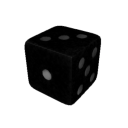
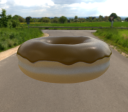
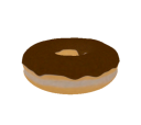
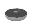
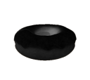
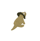
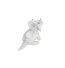
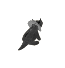
Figure 6. We demonstrate the informativeness of our fast approximate entropy for other inverse rendering frameworks (in this case, Mitsuba). We interleave ground truth properties and properties estimated with Mitsuba (base color, roughness, metallicity). On the right, we show the average estimation error followed by our entropy estimation, which is independent of Mitsuba’s estimation. We observe that low entropy is indicative of lower error, suggesting that it captures the sufficiency of information in the input signal. On the dice example (top row), the ‘one’-face is lit less than other faces and we observe highlights with lower intensity, leading to higher entropy. While we still recover the white albedo correctly, the estimation of roughness and metallicity for the dot has a high error. Similarly, the inside and lower parts of the doughnut are less observed and not lit by strong light sources. Again, entropy is high in regions of high error (especially in metallicity). The triceratops collar is down-facing and not well-lit and our entropy captures the lack of observation that leads to high error in the metallicity part.

Table 3. Comparing correlation between entropy computed with Mitsuba and our approximations.

	Entropy Mitsuba $\uparrow$	Time
Entropy Mitsuba	$1.00\pm 0.00$	$15$m
Entropy angular	$0.90\pm 0.05$	$2.91$s
Entropy power spectrum	$0.89\pm 0.06$	$0.0011$s

5.5. Ablations

Our ablations serve two goals. First, we want to validate that our proposed improvements to Ramamoorthi and Hanrahan (2001) make a significant difference. Second, we would like to study the sensitivity of the approach to some hyperparameters (e.g. regularizer weight, number of spherical harmonics degrees). We vary our method and report the results on Stanford ORB and the synthetic dataset. Further ablations on spherical-harmonics fitting are in the Appendix.

5.5.1. BRDF model variants

To understand whether our proposed improvements to the BRDF model by Ramamoorthi and Hanrahan (2001) result in higher-quality acquisition results, we study variants of our model with and without the shadowing and masking terms. We run our ablations with a constant weight on all the samples. The results on Stanford ORB are presented in Table 4. We observe that the shadowing- and masking terms improve the results independently and we get the best results with both.

Table 4. We ablate the different components of the BRDF. For this ablation we do not apply a cosine weighting to the samples, better highlighting the impact of the shadowing and masking terms.

		Stanford ORB					Synthetic
Shadowing	Masking	PSNR-H$\uparrow$	PSNR-L$\uparrow$	SSIM$\uparrow$	LPIPS$\downarrow$	Time	MSE	Time
-	-	$25.646$	$32.809$	$0.973$	$0.035$	$1.09$s	$0.16$	$\mathbf{2.57}$s
✓	-	$26.245$	$33.399$	$0.975$	$0.034$	$1.21$s	$0.14$	$2.81$s
-	✓	$26.070$	$33.101$	$0.974$	$0.035$	$1.19$s	$0.13$	$2.89$s
✓	✓	$\mathbf{26.411}$	$\mathbf{33.557}$	$\mathbf{0.975}$	$\mathbf{0.034}$	$1.31$s	$\mathbf{0.12}$	$3.14$s

5.5.2. Convolutional only vs Directional

One of the main benefits of our method is that we can study the effect of the BRDF fully in the spherical harmonics domain. We can perform the full BRDF recovery procedure in the spherical harmonic domain or the power spectrum domain, as done for our initialization and uncertainty. We show the impact of evaluating the BRDF parameters from the power spectrum in row four of Table 1, compared to running our our mixed frequency-directional optimization (third row). As these approximations do not account for effects such as Fresnel or shadowing/masking, we observe lower appearance matching, as expected. The approximations however still result in a very good appearance match and extremely fast computation. Most of the reported timings in Table 1 reflects the fitting of the spherical harmonics, which only has to be done once, letting us easily explore hundreds to thousands of possible parameter combinations in a fraction of a second to compute uncertainty.

5.6. Applications

In our applications, we show how fast acquisition and uncertainty can be used in (SV)BRDF capture to improve results, and guide understanding of error.

Table 5. We apply our results as an initialization for a short fine-tuning pass using gradient descent with a differentiable path tracer (Mitsuba): we use only $1$ epoch with $16$ samples per pixel for the first three rows and $2$ epochs with $32$ samples per pixel for the fourth row. The final row shows the result of a full optimization for Mitsuba.

Initialization	PSNR-H$\uparrow$	PSNR-L$\uparrow$	SSIM$\uparrow$	LPIPS$\downarrow$	Total time
Constant	$24.339$	$30.558$	$0.969$	$0.047$	$14.74$s
Ours - Spectrum Only	$25.745$	$33.158$	$0.975$	$0.033$	$16.29$s
Ours	$27.038$	$34.560$	$\mathbf{0.978}$	$0.030$	$19.87$s
Ours (2 epochs)	$\mathbf{27.199}$	$\mathbf{34.770}$	$\mathbf{0.978}$	$\mathbf{0.029}$	$33.39$s
Full optimization - Constant	$26.595$	$34.185$	$0.977$	$0.032$	$69.96$s

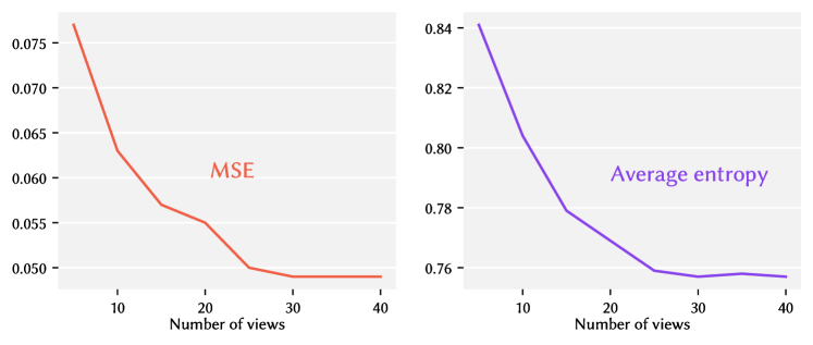
Figure 8. Plots of MSE and Entropy for varying input view counts on the synthetic benchmark with the Rural Road environment, showing that entropy can be used as a proxy of average MSE for a given set of views.

5.6.1. Initialization

In the comparisons, our method demonstrated a fast and high-quality estimate of BRDF parameters. However, there is still benefit to finetuning our results with a differentiable path tracer. Such a step could finetune parts of the material that are affected by global illumination (e.g., in corners, or near highly reflective surfaces). In this experiment, we show the benefit of this approach by initializing material textures with the results from our method and optimizing them with Mitsuba for one epoch and only $16$ samples per pixel (half the samples we used for the other experiments). This finetuning pass only costs $14$s, for a total of $20$s combined with out method as initialization. This is over three times faster than the $70$s required without this initialization (Table 1). The results in Table 5 show that the combination of our approach and a finetuning pass with Mitsuba for one or two epochs achieves better performance than only using Mitsuba (+$0.5$dB PSNR-H, PSNR-L) for less than a third of the time. We also surpass the results for only our method, which is to be expected.

Table 6. We combine the optimization results from multiple environments into one texture by using the parameter with the lowest certainty. We present the MSE in the following way: Average (Base Color, Roughness, Metallicity)

	MSE Synthetic
Average	$0.04$ ($0.01$, $0.03$, $0.07$)
$\arg\min$ Entropy	$0.03$ ($0.01$, $0.02$, $0.06$)

5.6.2. Sharing information

Points on the surface with low entropy have reasonable certainty and will likely exhibit lower error than parts with high entropy. We can use this information to select the best conditions to recover BRDF parameters, for example from different lighting setups. As a proof of concept, we merge the texture maps from the synthetic scenes based on entropy: for every texel, we use the parameters from the environment with the lowest entropy at that texel. The result in Table 6 shows that this simple approach beats the average over separate environments by $25\%$. The score is equal to the best-performing environment in Table 2. With this, we are able to select the best parameters without knowing the ground-truth. We believe that this approach would yield even stronger results in the context of more complementary environments.

5.6.3. Guiding capture

Entropy can be applied during capture as a measure to define the most informative views. If a view decreases entropy, it’s useful; if it does not, we could discard it. It is difficult to know what information a view will add without knowing its contents. A solution to this could be to compute an expected decrease in entropy (information gain) in case potential views are not known. Since this is not part of our core contribution, we leave this for future work. Instead, we show that entropy is useful to measure the informativeness of views. We ran the synthetic benchmark for one environment (Rural Road) and randomly drop out views for every optimization. In Figure 8, we show the corresponding average MSE over all shapes and channels and the average entropy over all shapes. We observe a clear relationship between the MSE and entropy, demonstrating that we can use entropy as a proxy for the expected success of an optimization. If one were to use entropy in real time, the alternatives to the power spectrum approximation quickly become tedious to use: for every frame that is considered, one would either have to wait a couple of seconds or minutes to compute the entropy (Table 3).

6. Challenges and conclusion

In summary, we present a material acquisition and uncertainty estimation method for multi-view capture of objects using a frequency domain analysis. We do so through efficient spherical harmonics fitting and a power spectrum approximation that lets us efficiently compute the error associated with varying material parameters for a surface. By interpreting this error as a likelihood function, we can use entropy as a measure of uncertainty. The results indicate correlation of low entropy with low error, both quantitatively and qualitatively. We show that entropy can be a useful proxy for acquisition quality. We also propose a way to take into account shadowing and masking to better reconstruct the target appearance and estimated properties, compared to the existing signal processing framework for inverse rendering. Our method yields results that are on par with the state-of-the-art for a $13$x speedup in optimization and, combined with state-of-the-art, yields improved results for less than a third of the time.

We see the following challenges for future work. Our method requires HDR images as input, because the truncation applied for LDR images could introduce frequencies that are not present in the original signal. To make our method more accessible for use with LDR images, it is of interest to study how to use spherical harmonics decompositions on LDR images. This could be implemented, for example, as an amendment to the least-squares fitting procedure. Our current implementation only considers direct illumination, neglecting self-illumination and self-shadowing which may appear in challenging concave objects; our method could be extended to take them into account with a ray tracer, as our core theoretical and algorithmic contributions are defined for a general directional radiance field for points in space. Nonetheless, our method produces accurate estimations of materials and can be used as an initialization for more complete (and slower) differentiable renderer (Jakob et al., 2022) for areas showing effects that we do not currently support.

We believe that our renewed exploration and improvement of the frequency-based model demonstrates the merits of this framework. We are excited about further applications that take advantage of entropy as a measure of uncertainty for material recovery.

References

- (1)
- Aittala et al. (2016) Miika Aittala, Timo Aila, and Jaakko Lehtinen. 2016. Reflectance modeling by neural texture synthesis. ACM Trans. Graph. 35, 4, Article 65 (jul 2016), 13 pages. https://doi.org/10.1145/2897824.2925917
- Aittala et al. (2013) Miika Aittala, Tim Weyrich, and Jaakko Lehtinen. 2013. Practical SVBRDF capture in the frequency domain. ACM Trans. Graph. 32, 4 (2013), 110–1.
- Aittala et al. (2015) Miika Aittala, Tim Weyrich, Jaakko Lehtinen, et al. 2015. Two-shot SVBRDF capture for stationary materials. ACM Trans. Graph. 34, 4 (2015), 110–1.
- Bi et al. (2020) Sai Bi, Zexiang Xu, Pratul P. Srinivasan, Ben Mildenhall, Kalyan Sunkavalli, Milos Hasan, Yannick Hold-Geoffroy, David J. Kriegman, and Ravi Ramamoorthi. 2020. Neural Reflectance Fields for Appearance Acquisition. abs/2008.03824 (2020). arXiv:2008.03824 https://arxiv.org/abs/2008.03824
- Boss et al. (2021a) Mark Boss, Raphael Braun, Varun Jampani, Jonathan T Barron, Ce Liu, and Hendrik Lensch. 2021a. Nerd: Neural reflectance decomposition from image collections. In Proceedings of the IEEE/CVF International Conference on Computer Vision. 12684–12694.
- Boss et al. (2021b) Mark Boss, Varun Jampani, Raphael Braun, Ce Liu, Jonathan Barron, and Hendrik Lensch. 2021b. Neural-pil: Neural pre-integrated lighting for reflectance decomposition. Advances in Neural Information Processing Systems 34 (2021), 10691–10704.
- Boss et al. (2020) Mark Boss, Varun Jampani, Kihwan Kim, Hendrik Lensch, and Jan Kautz. 2020. Two-shot spatially-varying brdf and shape estimation. In Proceedings of the IEEE/CVF Conference on Computer Vision and Pattern Recognition. 3982–3991.
- Burley and Studios (2012) Brent Burley and Walt Disney Animation Studios. 2012. Physically-based shading at disney. In Acm Siggraph, Vol. 2012. vol. 2012, 1–7.
- Chang et al. (2023) Wesley Chang, Venkataram Sivaram, Derek Nowrouzezahrai, Toshiya Hachisuka, Ravi Ramamoorthi, and Tzu-Mao Li. 2023. Parameter-space ReSTIR for Differentiable and Inverse Rendering. In ACM SIGGRAPH 2023 Conference Proceedings (Los Angeles, CA, USA) (SIGGRAPH ’23). Association for Computing Machinery, New York, NY, USA, 10 pages. https://doi.org/10.1145/3588432.3591512
- Deschaintre et al. (2018) Valentin Deschaintre, Miika Aittala, Fredo Durand, George Drettakis, and Adrien Bousseau. 2018. Single-image svbrdf capture with a rendering-aware deep network. ACM Transactions on Graphics (ToG) 37, 4 (2018), 1–15.
- Deschaintre et al. (2019) Valentin Deschaintre, Miika Aittala, Frédo Durand, George Drettakis, and Adrien Bousseau. 2019. Flexible svbrdf capture with a multi-image deep network. In Computer graphics forum, Vol. 38. Wiley Online Library, 1–13.
- Deschaintre et al. (2020) Valentin Deschaintre, George Drettakis, and Adrien Bousseau. 2020. Guided Fine-Tuning for Large-Scale Material Transfer. Computer Graphics Forum (Proceedings of the Eurographics Symposium on Rendering) 39, 4 (2020). http://www-sop.inria.fr/reves/Basilic/2020/DDB20
- Deschaintre et al. (2021) Valentin Deschaintre, Yiming Lin, and Abhijeet Ghosh. 2021. Deep polarization imaging for 3D shape and SVBRDF acquisition. In Proceedings of the IEEE/CVF Conference on Computer Vision and Pattern Recognition. 15567–15576.
- Dong et al. (2014) Yue Dong, Guojun Chen, Pieter Peers, Jiawan Zhang, and Xin Tong. 2014. Appearance-from-motion: Recovering spatially varying surface reflectance under unknown lighting. ACM Transactions on Graphics (TOG) 33, 6 (2014), 1–12.
- Driscoll and Healy (1994) J.R. Driscoll and D.M. Healy. 1994. Computing Fourier Transforms and Convolutions on the 2-Sphere. Advances in Applied Mathematics 15, 2 (1994), 202–250. https://doi.org/10.1006/aama.1994.1008
- Dupuy and Jakob (2018) Jonathan Dupuy and Wenzel Jakob. 2018. An Adaptive Parameterization for Efficient Material Acquisition and Rendering. Transactions on Graphics (Proceedings of SIGGRAPH Asia) 37, 6 (Nov. 2018), 274:1–274:18. https://doi.org/10.1145/3272127.3275059
- Durand et al. (2005) Frédo Durand, Nicolas Holzschuch, Cyril Soler, Eric Chan, and François X. Sillion. 2005. A frequency analysis of light transport. ACM Trans. Graph. 24, 3 (jul 2005), 1115–1126. https://doi.org/10.1145/1073204.1073320
- Engelhardt et al. (2024) Andreas Engelhardt, Amit Raj, Mark Boss, Yunzhi Zhang, Abhishek Kar, Yuanzhen Li, Deqing Sun, Ricardo Martin Brualla, Jonathan T. Barron, Hendrik P. A. Lensch, and Varun Jampani. 2024. SHINOBI: SHape and Illumination using Neural Object Decomposition via BRDF Optimization In-the-wild. ArXiv e-prints (2024).
- Fan et al. (2023) Chongrui Fan, Yiming Lin, and Abhijeet Ghosh. 2023. Deep Shape and SVBRDF Estimation using Smartphone Multi-lens Imaging. Computer Graphics Forum (2023). https://doi.org/10.1111/cgf.14972
- Fleming et al. (2003) Roland W. Fleming, Ron O. Dror, and Edward H. Adelson. 2003. Real-world illumination and the perception of surface reflectance properties. Journal of Vision 3, 5 (07 2003), 3–3. https://doi.org/10.1167/3.5.3 arXiv:https://arvojournals.org/arvo/content_public/journal/jov/932825/jov-3-5-3.pdf
- Gal and Ghahramani (2016) Yarin Gal and Zoubin Ghahramani. 2016. Dropout as a bayesian approximation: Representing model uncertainty in deep learning. In international conference on machine learning. PMLR, 1050–1059.
- Gao et al. (2019) Duan Gao, Xiao Li, Yue Dong, Pieter Peers, Kun Xu, and Xin Tong. 2019. Deep inverse rendering for high-resolution SVBRDF estimation from an arbitrary number of images. ACM Trans. Graph. 38, 4 (2019), 134–1.
- Ghosh et al. (2007) Abhijeet Ghosh, Shruthi Achutha, Wolfgang Heidrich, and Matthew O’Toole. 2007. BRDF Acquisition with Basis Illumination. In 2007 IEEE 11th International Conference on Computer Vision. IEEE, Rio de Janeiro, Brazil, 1–8. https://doi.org/10.1109/ICCV.2007.4408935
- Goli et al. (2024) Lily Goli, Cody Reading, Silvia Sellán, Alec Jacobson, and Andrea Tagliasacchi. 2024. Bayes’ Rays: Uncertainty Quantification in Neural Radiance Fields. CVPR (2024).
- Guo et al. (2021) Jie Guo, Shuichang Lai, Chengzhi Tao, Yuelong Cai, Lei Wang, Yanwen Guo, and Ling-Qi Yan. 2021. Highlight-aware two-stream network for single-image SVBRDF acquisition. ACM Trans. Graph. 40, 4, Article 123 (jul 2021), 14 pages. https://doi.org/10.1145/3450626.3459854
- Guo et al. (2020) Yu Guo, Cameron Smith, Miloš Hašan, Kalyan Sunkavalli, and Shuang Zhao. 2020. Materialgan: reflectance capture using a generative svbrdf model. arXiv preprint arXiv:2010.00114 (2020).
- Henzler et al. (2021) Philipp Henzler, Valentin Deschaintre, Niloy J Mitra, and Tobias Ritschel. 2021. Generative Modelling of BRDF Textures from Flash Images. ACM Trans Graph (Proc. SIGGRAPH Asia) 40, 6 (2021).
- Hwang et al. (2022) Inseung Hwang, Daniel S. Jeon, Adolfo Muñoz, Diego Gutierrez, Xin Tong, and Min H. Kim. 2022. Sparse Ellipsometry: Portable Acquisition of Polarimetric SVBRDF and Shape with Unstructured Flash Photography. ACM Transactions on Graphics (Proc. SIGGRAPH 2022) 41, 4 (2022).
- Jakob et al. (2022) Wenzel Jakob, Sébastien Speierer, Nicolas Roussel, Merlin Nimier-David, Delio Vicini, Tizian Zeltner, Baptiste Nicolet, Miguel Crespo, Vincent Leroy, and Ziyi Zhang. 2022. Mitsuba 3 renderer. https://mitsuba-renderer.org.
- Jaynes (1957) Edwin T Jaynes. 1957. Information theory and statistical mechanics. Physical review 106, 4 (1957), 620.
- Jin et al. (2023) Haian Jin, Isabella Liu, Peijia Xu, Xiaoshuai Zhang, Songfang Han, Sai Bi, Xiaowei Zhou, Zexiang Xu, and Hao Su. 2023. TensoIR: Tensorial Inverse Rendering. arXiv:2304.12461
- Kerbl et al. (2023) Bernhard Kerbl, Georgios Kopanas, Thomas Leimkühler, and George Drettakis. 2023. 3D Gaussian Splatting for Real-Time Radiance Field Rendering. ACM Transactions on Graphics 42, 4 (July 2023). https://repo-sam.inria.fr/fungraph/3d-gaussian-splatting/
- Kuang et al. (2023) Zhengfei Kuang, Yunzhi Zhang, Hong-Xing Yu, Samir Agarwala, Shangzhe Wu, and Jiajun Wu. 2023. Stanford-ORB: A Real-World 3D Object Inverse Rendering Benchmark. arXiv:2310.16044 [cs.CV]
- Laine et al. (2020) Samuli Laine, Janne Hellsten, Tero Karras, Yeongho Seol, Jaakko Lehtinen, and Timo Aila. 2020. Modular Primitives for High-Performance Differentiable Rendering. ACM Transactions on Graphics 39, 6 (2020).
- Lensch et al. (2003a) Hendrik Lensch, Jan Kautz, Michael Goesele, Wolfgang Heidrich, and Hans-Peter Seidel. 2003a. Image-based Reconstruction of Spatial Appearance and Geometric Detail. ACM Transactions on Graphics (TOG) 22 (04 2003), 234–257. https://doi.org/10.1145/636886.636891
- Lensch et al. (2003b) Hendrik P.A. Lensch, Jochen Lang, Asla M. Sá, and Hans-Peter Seidel. 2003b. Planned Sampling of Spatially Varying BRDFs. Computer Graphics Forum 22, 3 (2003), 473–482. https://doi.org/10.1111/1467-8659.00695 arXiv:https://onlinelibrary.wiley.com/doi/pdf/10.1111/1467-8659.00695
- Li et al. (2017) Xiao Li, Yue Dong, Pieter Peers, and Xin Tong. 2017. Modeling surface appearance from a single photograph using self-augmented convolutional neural networks. ACM Transactions on Graphics (ToG) 36, 4 (2017), 1–11.
- Li et al. (2018) Zhengqin Li, Zexiang Xu, Ravi Ramamoorthi, Kalyan Sunkavalli, and Manmohan Chandraker. 2018. Learning to reconstruct shape and spatially-varying reflectance from a single image. ACM Transactions on Graphics (TOG) 37, 6 (2018), 1–11.
- Loubet et al. (2019) Guillaume Loubet, Nicolas Holzschuch, and Wenzel Jakob. 2019. Reparameterizing Discontinuous Integrands for Differentiable Rendering. Transactions on Graphics (Proceedings of SIGGRAPH Asia) 38, 6 (Dec. 2019). https://doi.org/10.1145/3355089.3356510
- Mao et al. (2023) Shi Mao, Chenming Wu, Zhelun Shen, and Liangjun Zhang. 2023. NeuS-PIR: Learning Relightable Neural Surface using Pre-Integrated Rendering. arXiv preprint arXiv:2306.07632 (2023).
- Martin et al. (2022) Rosalie Martin, Arthur Roullier, Romain Rouffet, Adrien Kaiser, and Tamy Boubekeur. 2022. MaterIA: Single Image High-Resolution Material Capture in the Wild. Computer Graphics Forum (Proc. EUROGRAPHICS 2022) to appear, to appear (2022), to appear.
- Mildenhall et al. (2020) Ben Mildenhall, Pratul P. Srinivasan, Matthew Tancik, Jonathan T. Barron, Ravi Ramamoorthi, and Ren Ng. 2020. NeRF: Representing Scenes as Neural Radiance Fields for View Synthesis. In ECCV.
- Munkberg et al. (2022) Jacob Munkberg, Jon Hasselgren, Tianchang Shen, Jun Gao, Wenzheng Chen, Alex Evans, Thomas Müller, and Sanja Fidler. 2022. Extracting triangular 3d models, materials, and lighting from images. In Proceedings of the IEEE/CVF Conference on Computer Vision and Pattern Recognition. 8280–8290.
- Nam et al. (2018) Giljoo Nam, Joo Ho Lee, Diego Gutierrez, and Min H. Kim. 2018. Practical SVBRDF Acquisition of 3D Objects with Unstructured Flash Photography. ACM Transactions on Graphics (Proc. SIGGRAPH Asia 2018) 37, 6 (2018), 267:1–12. https://doi.org/10.1145/3272127.3275017
- Nicolet et al. (2021) Baptiste Nicolet, Alec Jacobson, and Wenzel Jakob. 2021. Large Steps in Inverse Rendering of Geometry. ACM Transactions on Graphics (Proceedings of SIGGRAPH Asia) 40, 6 (Dec. 2021). https://doi.org/10.1145/3478513.3480501
- Nicolet et al. (2023) Baptiste Nicolet, Fabrice Rousselle, Jan Novák, Alexander Keller, Wenzel Jakob, and Thomas Müller. 2023. Recursive Control Variates for Inverse Rendering. Transactions on Graphics (Proceedings of SIGGRAPH) 42, 4 (Aug. 2023). https://doi.org/10.1145/3592139
- Nimier-David et al. (2021) Merlin Nimier-David, Zhao Dong, Wenzel Jakob, and Anton Kaplanyan. 2021. Material and Lighting Reconstruction for Complex Indoor Scenes with Texture-space Differentiable Rendering. In Eurographics Symposium on Rendering - DL-only Track, Adrien Bousseau and Morgan McGuire (Eds.). The Eurographics Association. https://doi.org/10.2312/sr.20211292
- Nimier-David et al. (2022) Merlin Nimier-David, Thomas Müller, Alexander Keller, and Wenzel Jakob. 2022. Unbiased Inverse Volume Rendering with Differential Trackers. ACM Trans. Graph. 41, 4, Article 44 (July 2022), 20 pages. https://doi.org/10.1145/3528223.3530073
- Nimier-David et al. (2020) Merlin Nimier-David, Sébastien Speierer, Benoît Ruiz, and Wenzel Jakob. 2020. Radiative Backpropagation: An Adjoint Method for Lightning-Fast Differentiable Rendering. Transactions on Graphics (Proceedings of SIGGRAPH) 39, 4 (July 2020). https://doi.org/10.1145/3386569.3392406
- Nimier-David et al. (2019) Merlin Nimier-David, Delio Vicini, Tizian Zeltner, and Wenzel Jakob. 2019. Mitsuba 2: A Retargetable Forward and Inverse Renderer. Transactions on Graphics (Proceedings of SIGGRAPH Asia) 38, 6 (Dec. 2019). https://doi.org/10.1145/3355089.3356498
- Pharr et al. (2023) Matt Pharr, Wenzel Jakob, and Greg Humphreys. 2023. Physically based rendering: From theory to implementation. MIT Press.
- Ramamoorthi and Hanrahan (2001) Ravi Ramamoorthi and Pat Hanrahan. 2001. A signal-processing framework for inverse rendering. In Proceedings of the 28th annual conference on Computer graphics and interactive techniques (SIGGRAPH ’01). Association for Computing Machinery, New York, NY, USA, 117–128. https://doi.org/10.1145/383259.383271
- Rodriguez-Pardo et al. (2023) C. Rodriguez-Pardo, H. Dominguez-Elvira, D. Pascual-Hernandez, and E. Garces. 2023. UMat: Uncertainty-Aware Single Image High Resolution Material Capture. In 2023 IEEE/CVF Conference on Computer Vision and Pattern Recognition (CVPR). IEEE Computer Society, Los Alamitos, CA, USA, 5764–5774. https://doi.org/10.1109/CVPR52729.2023.00558
- Rosu and Behnke (2023) Radu Alexandru Rosu and Sven Behnke. 2023. PermutoSDF: Fast Multi-View Reconstruction with Implicit Surfaces using Permutohedral Lattices. In IEEE/CVF Conference on Computer Vision and Pattern Recognition (CVPR).
- Shah et al. (2023) Viraj Shah, Svetlana Lazebnik, and Julien Philip. 2023. JoIN: Joint GANs Inversion for Intrinsic Image Decomposition. arXiv (2023).
- Shi et al. (2020) Liang Shi, Beichen Li, Miloš Hašan, Kalyan Sunkavalli, Tamy Boubekeur, Radomir Mech, and Wojciech Matusik. 2020. MATch: Differentiable Material Graphs for Procedural Material Capture. ACM Trans. Graph. 39, 6 (Dec. 2020), 1–15.
- Spielberg et al. (2023) Andrew Spielberg, Fangcheng Zhong, Konstantinos Rematas, Krishna Murthy Jatavallabhula, Cengiz Öztireli, Tzu-Mao Li, and Derek Nowrouzezahrai. 2023. Differentiable Visual Computing for Inverse Problems and Machine Learning. CoRR abs/2312.04574 (2023). https://doi.org/10.48550/ARXIV.2312.04574 arXiv:2312.04574
- Srinivasan et al. (2021) Pratul P Srinivasan, Boyang Deng, Xiuming Zhang, Matthew Tancik, Ben Mildenhall, and Jonathan T Barron. 2021. Nerv: Neural reflectance and visibility fields for relighting and view synthesis. In Proceedings of the IEEE/CVF Conference on Computer Vision and Pattern Recognition. 7495–7504.
- Sun et al. (2023) Cheng Sun, Guangyan Cai, Zhengqin Li, Kai Yan, Cheng Zhang, Carl Marshall, Jia-Bin Huang, Shuang Zhao, and Zhao Dong. 2023. Neural-PBIR Reconstruction of Shape, Material, and Illumination. In Proceedings of the IEEE/CVF International Conference on Computer Vision. 18046–18056.
- Torrance and Sparrow (1967) K. E. Torrance and E. M. Sparrow. 1967. Theory for Off-Specular Reflection From Roughened Surfaces. J. Opt. Soc. Am. 57, 9 (Sep 1967), 1105–1114. https://doi.org/10.1364/JOSA.57.001105
- Trowbridge and Reitz (1975) TS Trowbridge and Karl P Reitz. 1975. Average irregularity representation of a rough surface for ray reflection. JOSA 65, 5 (1975), 531–536.
- Vecchio et al. (2023) Giuseppe Vecchio, Rosalie Martin, Arthur Roullier, Adrien Kaiser, Romain Rouffet, Valentin Deschaintre, and Tamy Boubekeur. 2023. ControlMat: Controlled Generative Approach to Material Capture. arXiv preprint arXiv:2309.01700 (2023).
- Vicini et al. (2022) Delio Vicini, Sébastien Speierer, and Wenzel Jakob. 2022. Differentiable Signed Distance Function Rendering. Transactions on Graphics (Proceedings of SIGGRAPH) 41, 4 (July 2022), 125:1–125:18. https://doi.org/10.1145/3528223.3530139
- Walter et al. (2007) Bruce Walter, Stephen R Marschner, Hongsong Li, and Kenneth E Torrance. 2007. Microfacet models for refraction through rough surfaces. In Proceedings of the 18th Eurographics conference on Rendering Techniques. 195–206.
- Wieczorek and Meschede (2018) Mark A. Wieczorek and Matthias Meschede. 2018. SHTools: Tools for Working with Spherical Harmonics. Geochemistry, Geophysics, Geosystems 19, 8 (2018), 2574–2592. https://doi.org/10.1029/2018GC007529 arXiv:https://agupubs.onlinelibrary.wiley.com/doi/pdf/10.1029/2018GC007529
- Wu et al. (2023a) Haoqian Wu, Zhipeng Hu, Lincheng Li, Yongqiang Zhang, Changjie Fan, and Xin Yu. 2023a. NeFII: Inverse Rendering for Reflectance Decomposition with Near-Field Indirect Illumination. In Proceedings of the IEEE/CVF Conference on Computer Vision and Pattern Recognition. 4295–4304.
- Wu et al. (2023b) Liwen Wu, Rui Zhu, Mustafa B Yaldiz, Yinhao Zhu, Hong Cai, Janarbek Matai, Fatih Porikli, Tzu-Mao Li, Manmohan Chandraker, and Ravi Ramamoorthi. 2023b. Factorized Inverse Path Tracing for Efficient and Accurate Material-Lighting Estimation. In Proceedings of the IEEE/CVF International Conference on Computer Vision. 3848–3858.
- Xu et al. (2023) Peiyu Xu, Sai Bangaru, Tzu-Mao Li, and Shuang Zhao. 2023. Warped-Area Reparameterization of Differential Path Integrals. ACM Trans. Graph. 42, 6 (2023), 213:1–213:18.
- Xu et al. (2016) Zexiang Xu, Jannik Boll Nielsen, Jiyang Yu, Henrik Wann Jensen, and Ravi Ramamoorthi. 2016. Minimal BRDF sampling for two-shot near-field reflectance acquisition. ACM Transactions on Graphics (TOG) 35, 6 (2016), 1–12.
- Yan et al. (2022) Kai Yan, Christoph Lassner, Brian Budge, Zhao Dong, and Shuang Zhao. 2022. Efficient Estimation of Boundary Integrals for Path-Space Differentiable Rendering. ACM Trans. Graph. 41, 4 (2022), 123:1–123:13.
- Zhang et al. (2021a) Kai Zhang, Fujun Luan, Qianqian Wang, Kavita Bala, and Noah Snavely. 2021a. Physg: Inverse rendering with spherical gaussians for physics-based material editing and relighting. In Proceedings of the IEEE/CVF Conference on Computer Vision and Pattern Recognition. 5453–5462.
- Zhang et al. (2021b) Xiuming Zhang, Pratul P Srinivasan, Boyang Deng, Paul Debevec, William T Freeman, and Jonathan T Barron. 2021b. Nerfactor: Neural factorization of shape and reflectance under an unknown illumination. ACM Transactions on Graphics (ToG) 40, 6 (2021), 1–18.
- Zhang et al. (2023) Youjia Zhang, Teng Xu, Junqing Yu, Yuteng Ye, Yanqing Jing, Junle Wang, Jingyi Yu, and Wei Yang. 2023. Nemf: Inverse volume rendering with neural microflake field. In Proceedings of the IEEE/CVF International Conference on Computer Vision. 22919–22929.
- Zheng et al. (2019) Yi Zheng, Kai Wei, Bin Liang, Ying Li, and Xinhui Chu. 2019. Zernike like functions on spherical cap: principle and applications in optical surface fitting and graphics rendering. Optics Express 27, 26 (Dec. 2019), 37180. https://doi.org/10.1364/OE.27.037180
- Zhou et al. (2023) Xilong Zhou, Miloš Hašan, Valentin Deschaintre, Paul Guerrero, Kalyan Sunkavalli, and Nima Khademi Kalantari. 2023. A Semi-Procedural Convolutional Material Prior. In Computer Graphics Forum. Wiley Online Library.
- Zhou and Kalantari (2021) Xilong Zhou and Nima Khademi Kalantari. 2021. Adversarial Single-Image SVBRDF Estimation with Hybrid Training. Computer Graphics Forum (2021).
- Zhou and Khademi Kalantari (2022) Xilong Zhou and Nima Khademi Kalantari. 2022. Look-Ahead Training with Learned Reflectance Loss for Single-Image SVBRDF Estimation. ACM Transactions on Graphics 41, 6 (12 2022). https://doi.org/10.1145/3550454.3555495