Violation of $\gamma$ in Brans-Dicke gravity

Abstract

The Brans Class I solution in Brans-Dicke gravity is a staple in the study of gravitational theories beyond General Relativity. Discovered in 1961, it describes the exterior vacuum of a spherical Brans-Dicke star and is characterized by two adjustable parameters. Surprisingly, the relationship between these parameters and the properties of the star has not been rigorously established. In this Proceeding, we bridge this gap by deriving the complete exterior solution of Brans Class I, expressed in terms of the total energy and total pressure of the spherisymmetric gravity source. The solution allows for the exact derivation of all post-Newtonian parameters in Brans-Dicke gravity for far field regions of a spherical source. Particularly for the $\gamma$ parameter, instead of the conventional result $\gamma_{\,\text{PPN}}=\frac{\omega+1}{\omega+2}$, we obtain the analytical expression $\gamma_{\,\text{exact}}=\frac{\omega+1+(\omega+2)\,\Theta}{\omega+2+(\omega+1)\,\Theta}$ where $\Theta$ is the ratio of the total pressure $P_{\parallel}^{*}+2P_{\perp}^{*}$ and total energy $E^{*}$ contained within the mass source. Our non-perturbative $\gamma$ formula is valid for all field strengths and types of matter comprising the mass source. Consequently, observational constraints on $\gamma$ thus set joint bounds on $\omega$ and $\varTheta$, with the latter representing a global characteristic of the mass source. More broadly, our formula highlights the importance of pressure (when $\varTheta\neq 0$) in spherical Brans-Dicke stars, and potentially in stars within other modified theories of gravitation.

Background—Brans–Dicke gravity is the second most studied theory of gravitation besides General Relativity. It represents one of the simplest extensions of gravitational theory beyond GR [2]. It is characterized by an additional dynamical scalar field $\phi$ which, in the original vision of Brans and Dicke in 1961, acts like the inverse of a variable Newton ‘constant’ $G$. The scalar field has a kinetic term, governed by a (Brans-Dicke) parameter $\omega$ in the following gravitation action

$$S=\frac{1}{16\pi}\int d^{4}x\sqrt{-g}\left[\Phi\,\mathcal{R}-\frac{\omega}{\Phi}g^{\mu\nu}\partial_{\mu}\Phi\partial_{\nu}\Phi\right]$$ (1)

In the limit of infinite value for $\omega$, the kinetic term is generally said to be ‘frozen’, rendering $\Phi$ being a constant value everywhere. In this limit, if the field $\phi$ approaches its (non-zero) constant value in the rate $\mathcal{O}\left(1/\omega\right)$, the term $\frac{\omega}{\Phi}g^{\mu\nu}\partial_{\mu}\Phi\partial_{\nu}\Phi$ would approach zero at the rate $\mathcal{O}\left(1/\omega\right)$ and hence become negligible compared with the term $\Phi\,\mathcal{R}$, effectively recovering the classic Einstein–Hilbert action.

Together with its introduction [2], Brans also identified four classes of exact solutions in the static spherically symmetric (SSS) setup [3]. The derivation of the Brans solutions was explicitly carried out by Bronnikov in 1973 [5]. Of the four classes, only the Brans Class I is physically meaningful, however. It can recover the Schwarzschild solution in its parameter space.

For comparison with observations or experiments, Brans derived the Robertson (or Eddington-Robertson- Schiff) $\beta$ and $\gamma$ post-Newtonian (PN) parameters based on his Class I solution:

$$\beta_{\,\text{PPN}} =1$$ (2)

$$\gamma_{\,\text{PPN}} =\frac{\omega+1}{\omega+2}$$ (3)

The $\gamma$ parameter is important as it governs the amount of space-curvature produced by a body at rest and can be directly measured via the detection of light deflection and the Shapiro time delay. The parametrized post-Newtonian (PPN) $\gamma$ formula recovers the result $\gamma_{\,\text{GR}}=1$ known for GR in the limit of infinite $\omega$, in which the BD scalar field becomes constant everywhere. Current bounds using Solar System observations set the magnitude of $\omega$ to exceed $40,000$ [7].

We should emphasize that the “conventional” results (2) and (3) were derived under the assumption of zero pressure in the gravity source. It should be noted that these formulae can also be deduced directly from the PPN formalism for the Brans–Dicke action, without resorting to the Brans Class I solution [8, 6]. The PPN derivation relies on two crucial approximations: (i) weak field and (ii) slow motions. Regarding the latter approximation, an often under-emphasized point is that not only must the stars be in slow motion, but the microscopic constituents that comprise the stars must also be in slow motion. This translates to the requirement that the matter inside the stars exert low pressure, characterizing them as “Newtonian” stars.

The purpose of our paper is two-fold. Firstly, the analytical form for the exterior vacuum contains two adjustable parameters. The issue in determining them from the energy and pressure profiles inside the mass source has not been rigorously addressed in the literature. Establishing their relationships with the mass source would typically require the full machinery of the Tolman–Oppenheimer–Volkoff (TOV) equations tailored for Brans–Dicke gravity [9]. Moreover, solving the TOV equations, even in the simpler theory of GR, generally requires numerical methods except for a few isolated, unrealistic cases such as incompressible fluids. Therefore, at first glance, deriving a concrete expression for these relationships might seem elusive. Surprisingly, as we shall show in this Proceeding, this view is overly pessimistic. It turns out that the full machinery of the TOV equation is not necessary. Instead, only a subset of the field equation and the scalar equation of BD will be needed. This is because only two equations are required to fix the two free parameters of the exterior vacuum. We shall present a rigorous yet parsimonious derivation, which only became available through our recent publication [10].

Secondly, the complete solution enables the derivation of any PN parameters applicable for far-field regions in static spherical Brans-Dicke stars. As we shall show in this Proceeding, the derivation is non-perturbative and avoids the two PPN approximations requiring the weak field and the low pressure mentioned above.

The material presented in this Proceeding was developed during the preparation of our two recent papers [10, 11]. For a more detailed exposition of the conceptualization and technical points, we refer the reader to these papers.

The field equations and the energy-momentum tensor—It is well documented [5] that upon the Weyl mapping $\bigl{\{}\tilde{g}_{\mu\nu}:=\Phi\,g_{\mu\nu}$, $\tilde{\Phi}:=\ln\Phi\bigr{\}}$, the gravitational sector of the BD action can be brought to the Einstein frame as $\int d^{4}x\frac{\sqrt{-\tilde{g}}}{16\pi}\Bigl{[}\tilde{\mathcal{R}}-\left(\omega+3/2\right)\tilde{\nabla}^{\mu}\tilde{\Phi}\tilde{\nabla}_{\mu}\tilde{\Phi}\Bigr{]}$. The Einstein-frame BD scalar field $\tilde{\Phi}$ has a kinetic term with a signum determined by $(\omega+3/2)$. Unless stated otherwise, we shall restrict our consideration to the normal (“non-phantom”) case of $\omega>-3/2$, where the kinetic energy for $\tilde{\Phi}$ is positive.

The field equations are

$$R_{\mu\nu}-\frac{\omega}{\Phi^{2}}\partial_{\mu}\Phi\partial_{\nu}\Phi-\frac{1}{\Phi}\partial_{\mu}\partial_{\nu}\Phi+\Gamma_{\mu\nu}^{\lambda}\partial_{\lambda}\ln\Phi\ \ \ \ \ \ \ \ \ \$$

$$=\frac{8\pi}{\Phi}\left(T_{\mu\nu}-\frac{\omega+1}{2\omega+3}T\,g_{\mu\nu}\right)$$ (4)

$$\partial_{\mu}\left(\sqrt{-g}\,g^{\mu\nu}\partial_{\nu}\Phi\right)=\frac{8\pi}{2\omega+3}T\sqrt{-g}\ \ \ \ \ \ \ \ \,\ \ \ \ \ \ \$$ (5)

In the isotropic coordinate system which is static and spherically symmetric, the metric can be written as

$$ds^{2}=-A(r)dt^{2}+B(r)\left[dr^{2}+r^{2}\left(d\theta^{2}+\sin^{2}\theta d\varphi^{2}\right)\right]$$ (6)

It is straightforward to verify, from Eqs. (4)–(6), that the most general form for the energy-momentum tensor (EMT) in this setup is

$$T_{\mu}^{\nu} =\text{diag}\bigl{(}-\epsilon,\,p_{\|},\,p_{\bot},\,p_{\bot}\bigr{)}$$ (7)

where the energy density $\epsilon$, the radial pressure $p_{\parallel}$ and the tangential pressure $p_{\perp}$ are functions of $r$. Note that the EMT is anisotropic if $p_{\parallel}\neq p_{\perp}$. The trace of the EMT is

$$T=-\epsilon+p_{\parallel}+2p_{\perp}\,.$$ (8)

The Brans Class I vacuum solution outside a star—It is known that the scalar–metric for the vacuum is the Brans Class I solution (which satisfies Eqs. (5)–(4) for $T_{\mu\nu}=0$) [3]. In the isotropic coordinate system (6), the solution reads [3]

$$\left\{\begin{array}[]{l}A=\left(\frac{r-k}{r+k}\right)^{\frac{2}{\lambda}}\\ B=\left(1+\frac{k}{r}\right)^{4}\left(\frac{r-k}{r+k}\right)^{2-2\frac{\Lambda+1}{\lambda}}\\ \Phi=\left(\frac{r-k}{r+k}\right)^{\frac{\Lambda}{\lambda}}\end{array}\right.\ \ \ \ \ \text{for }r\geqslant r_{*}$$ (9)

where $r_{\ast}$ is the star’s radius, and

$$\lambda^{2}=\left(\Lambda+1\right)^{2}-\Lambda\left(1-\frac{\Lambda}{2}\omega\right)$$ (10)

Since $\lambda$ and $\Lambda$ are linked by (10), this solution involves two independent parameters, which one chooses to be $\left(k,\,\Lambda\right)$.

The field equations in the interior—For the region $r\leqslant r_{*}$, substituting metric (6) and the BD field $\Phi(r)$ into Eq. (5) and the $00-$component of Eq. (4) and using the EMT in Eq. (7), the functions $A(r)$, $B(r)$, $\Phi(r)$ satisfy the 2 following ordinary differential equations (ODEs):

$$\left(r^{2}\sqrt{AB}\Phi^{\prime}\right)^{\prime} =\frac{8\pi}{2\omega+3}\Bigl{[}-\epsilon+p_{\|}+2p_{\bot}\Bigr{]}r^{2}\sqrt{AB^{3}}$$ (11)

$$\left(r^{2}\Phi\sqrt{\frac{B}{A}}A^{\prime}\right)^{\prime} =16\pi\Bigl{[}\,\epsilon+\frac{\omega+1}{2\omega+3}\bigl{(}-\epsilon+p_{\|}+2p_{\bot}\bigr{)}\Bigr{]}r^{2}\sqrt{AB^{3}}$$ (12)

These equations offer the advantage of having both their left hand sides in exact derivative forms. Let us integrate Eqs. (11) and (12) from the star’s center, viz. $r=0$, to a coordinate $r>r_{\ast}$. The $\left(A,B,\Phi\right)$ functions are then given by (9) at $r$. For $r>r_{*}$, both $r^{2}\sqrt{AB}\Phi^{\prime}$ and $r^{2}\Phi\sqrt{\frac{B}{A}}A^{\prime}$ terms that enter the left hand sides of (11) and (12) are $r-$independent, since the right hand sides of these equations vanish in the exterior vacuum. On the other hand, regularity conditions inside the star impose $\Phi^{\prime}\left(0\right)=A^{\prime}\left(0\right)=0$ (i.e. no conic singularity) and finite values of the fields themselves. The calculation yields

$$\frac{k\,\Lambda}{\lambda} =\frac{4\pi}{2\omega+3}\int_{0}^{r_{\ast}}dr\,r^{2}\sqrt{AB^{3}}\Bigl{[}-\epsilon+p_{\|}+2p_{\bot}\Bigr{]}$$ (13)

and

$$\frac{k}{\lambda} =\frac{4\pi}{2\omega+3}\int_{0}^{r_{\ast}}dr\,r^{2}\sqrt{AB^{3}}\times$$

$$\ \ \ \ \ \ \ \ \ \ \ \ \ \ \ \ \ \Bigl{[}(\omega+2)\epsilon+(\omega+1)\bigl{(}p_{\|}+2p_{\bot}\bigr{)}\Bigr{]}\,.$$ (14)

Let us note that $r^{2}\sqrt{AB^{3}}$ is the square root of the determinant of the metric, up to the $\sin\theta$ term. (Accordingly, the integrals in the right hand sides of Eqs. (13) and (14) are invariant through radial coordinate transformations, since the combination $r^{2}\sqrt{AB^{3}}\sin\theta$ is equivalent to $\sqrt{-g}$.) We then can define the energy’s and pressures’ integrals by

$$E^{\ast} = 4\pi\int_{0}^{r_{\ast}}dr\,r^{2}\sqrt{AB^{3}}\,\epsilon$$ (15)

$$P_{\|}^{\ast} = 4\pi\int_{0}^{r_{\ast}}dr\,r^{2}\sqrt{AB^{3}}\,p_{\parallel}$$ (16)

$$P_{\bot}^{\ast} = 4\pi\int_{0}^{r_{\ast}}dr\,r^{2}\sqrt{AB^{3}}\,p_{\perp}\,.$$ (17)

Inserting in (13) and (14), we obtain

$$\frac{k}{\lambda}=E^{*}\Bigl{[}\frac{\omega+2}{2\omega+3}+\frac{\omega+1}{2\omega+3}\,\Theta\Bigr{]}$$ (18)

and

$$\Lambda=\frac{\Theta-1}{\omega+2+(\omega+1)\,\Theta}$$ (19)

in which the dimensionless parameter $\Theta$ is defined as

$$\Theta:=\frac{P_{\parallel}^{*}+2\,P_{\perp}^{*}}{E^{*}}\,.$$ (20)

Together with (9) and (10), these expressions provide a complete expression for the exterior spacetime and scalar field of a spherical BD star. To the best of our knowledge, this prescription was not made explicitly documented in the literature, until our recent works [11, 10].

For a perfect fluid, $p_{\|}=p_{\bot}\equiv p$, thence $P_{\|}^{\ast}=P_{\bot}^{\ast}\equiv P$. The equations (10), (13) and (14) fully determine the exterior solution (9) once the integrals (15)–(17) are known, with these integrals being fixed by the stellar internal structure model. This explicitly determines the particles’ motion outside the star, in both the remote and close to the star regions.

The ($\beta$, $\gamma$, $\delta$) PN parameters—In remote spatial regions, a static spherically symmetric metric in isotropic coordinates can be expanded as [8]:

$$ds^{2} =-\left(1-2\,\frac{M}{r}+2\beta\,\frac{M^{2}}{r^{2}}+\dots\right)dt^{2}$$

$$+\left(1+2\gamma\,\frac{M}{r}+\frac{3}{2}\delta\,\frac{M^{2}}{r^{2}}+\dots\right)\left(dr^{2}+r^{2}d\Omega^{2}\right)$$ (21)

in which $\beta$ and $\gamma$ are the Robertson (or Eddington-Robertson-Schiff) parameters, whereas $\delta$ is the second-order PN parameter (for both light and planetary like motions). It is straightforward to verify that the Schwarzschild metric yields

$$\beta_{\,\text{Schwd}}=\gamma_{\,\text{Schwd}}=\delta_{\,\text{Schwd}}=1$$ (22)

The metric in Eq. (9) can be re-expressed in the expansion form

$$ds^{2} =-\left(1-\frac{4}{\lambda}\frac{k}{\rho}+\frac{8}{\lambda^{2}}\frac{k^{2}}{r^{2}}+\dots\right)dt^{2}+\left(1+\frac{4}{\lambda}(1+\Lambda)\frac{k}{r}+\frac{2}{\lambda^{2}}\left(4(1+\Lambda)^{2}-\lambda^{2}\right)\frac{k^{2}}{r^{2}}+\dots\right)\left(dr^{2}+r^{2}d\Omega^{2}\right)$$ (23)

Comparing Eq. (21) against Eq. (23) and setting

$$M=2\,\frac{k}{\lambda}$$ (24)

we obtain

$$\beta_{\,\text{exact}} \ =\ 1$$ (25)

$$\gamma_{\,\text{exact}} \ =\ 1+\Lambda$$ (26)

$$\delta_{\,\text{exact}} \ =\ \frac{1}{3}\left(4(1+\Lambda)^{2}-\lambda^{2}\right)$$ (27)

where we have used the subscript “exact” as emphasis. Note that $\Lambda$ directly measures the deviation of the $\gamma$ parameters from GR ($\gamma_{\text{GR}}=1$). From Eq. (19), $\Lambda$ depends on both $\omega$ and $\Theta$. Finally, we arrive at

$$\gamma_{\,\text{exact}}\ =\ \frac{\omega+1+(\omega+2)\hskip 0.56917pt\varTheta}{\omega+2+(\omega+1)\hskip 0.56917pt\varTheta}$$ (28)

which can also be conveniently recast as

$$\gamma_{\,\text{exact}}\ =\ \frac{\gamma_{\,\text{PPN}}+\Theta}{1+\gamma_{\,\text{PPN}}\,\Theta}$$ (29)

by recalling that $\gamma_{\,\text{PPN}}=\frac{\omega+1}{\omega+2}$. To our knowledge, the closed-form expression (28) for $\gamma$ was absent in the literature, until our recent works [11, 10].

Regarding $\delta$:

$$\delta_{\,\text{exact}} =\frac{1}{\left[\omega+2+(\omega+1)\,\Theta\right]^{2}}\Bigl{[}\Bigl{(}\omega^{2}+\frac{3}{2}\omega+\frac{1}{3}\Bigr{)}$$

$$+\Bigl{(}2\omega^{2}+\frac{19}{3}\omega+\frac{13}{3}\Bigr{)}\Theta+\Bigl{(}\omega^{2}+\frac{25}{6}\omega+\frac{13}{3}\Bigr{)}\Theta^{2}\Bigr{]}$$ (30)

Figure 1 shows contour plots of $\gamma_{\,\text{exact}}$ and $\delta_{\,\text{exact}}$ as functions of $\gamma_{\,\text{PPN}}$ (i.e, $\frac{\omega+1}{\omega+2}$) and $\Theta$. In addition, with the aid of Eqs. (18) and (20), Eq. (24) produces the active gravitational mass

$$M =\frac{2\omega+4}{2\omega+3}\,E^{*}+\frac{2\omega+2}{2\omega+3}\,\left(P_{\parallel}^{*}+2P_{\bot}^{*}\right)$$ (31)

where the contribution of pressure to the active gravitational mass is evident [12, 13].

Degeneracy at ultra-high pressure—For $\Theta\rightarrow 1^{-}$, both $\gamma$ and $\delta$ go to 1, their GR counterpart values. Generally speaking, for $\Theta\rightarrow 1^{-}$, since $\Lambda\rightarrow 0$ and $\lambda\rightarrow 1$ regardless of $\omega$ (provided that $\omega\in(-3/2,+\infty)$), the value of $k$ approaches

$$k\rightarrow\frac{\omega+2}{2\omega+3}\,E^{*}+\frac{\omega+1}{2\omega+3}\,\left(P_{\parallel}^{*}+2P_{\bot}^{*}\right)$$ (32)

The $\omega-$dependence is thus absorbed into $k$, and the Brans Class I solution degenerates to the Schwarzschild solution

$$\left\{\begin{array}[]{l}A=\left(\frac{r-k}{r+k}\right)^{2}\\ B=\left(1+\frac{k}{r}\right)^{4}\\ \Phi=1\end{array}\right.\ \ \ \ \ \text{for }r\geqslant r_{*}$$ (33)

Therefore, ultra-relativistic Brans-Dicke stars are indistinguishable from their GR counterparts, as far as their exterior vacua are concerned. This fact can be explained by the following observation: For ultra-relativistic matter, the trace of the EMT vanishes, per Eq. (8). The scalar equation (5) then simplifies to $\square\,\Phi=0$ everywhere. Coupled with the regularity condition at the star center, this ensures a constant $\Phi$ throughout the spacetime which is now described by the Schwarzschild solution. Consequently, the scalar degree of freedom in BD gravity is suppressed in the ultra-relativistic limit. This prompts an intriguing possibility whether Birkhoff’s theorem is fully restored in this limit.

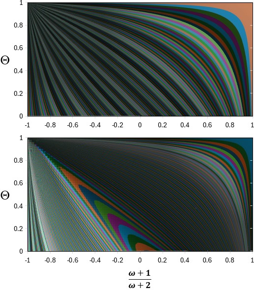
Figure 1: Contour plots of $\gamma_{\,\text{exact}}$ (upper panel) and $\delta_{\,\text{exact}}$ (lower panel) in terms of $\varTheta$ and $\frac{\omega+1}{\omega+2}$, for the range of $\varTheta\in[0,1]$ and $\omega\in(-3/2,+\infty)$, the latter corresponding to $\frac{\omega+1}{\omega+2}\in(-1,1)$. A measured $\gamma_{\,\text{exact}}\approx 1$ could mean $\frac{\omega+1}{\omega+2}\approx 1$ (i.e., $\omega\gg 1$) or $\varTheta\approx 1$ (i.e., ultra-relativistic matter). Contours are equally spaced in 0.01 increment. For a given contour in the upper panel, the corresponding value of $\gamma_{\,\text{exact}}$ can be read on the abscissa axis, where the contour intersects it. By measuring both $\gamma$ and $\delta$, the values of $\omega$ and $\Theta$ may be determined.

Discussions—Formulae (28) and (30) are the essential outcome of this Proceeding:

• Non-perturbative approach:   Our derivation is non-perturbative in nature. It makes use of the integrability of the $00-$component of the field equation (4), along with the scalar field equation (5).

• Parsimony:   Our derivation relies solely on the scalar field equation and the 00-component of the field equation, without the need for the full set of equations, specifically the $11-$ and $22-$ components of the field equation . The additional physical assumptions employed are the regularity at the star’s center and the existence of the star’s surface separating the interior and the exterior.

• Universality of results:   The final formulae, (28) and (30), hold for all field strengths and all types of matter (whether convective or non-convective, for example). We do not assume the matter comprising the stars to be a perfect fluid or isentropic.

• Higher-derivative characteristics:   In contrast to the one-parameter Schwarzschild metric, the Brans Class I solution depends on two parameters, i.e. the solution is not only defined by its gravitational mass, but also by a scalar mass besides the gravitational one [5]. The exterior BD vacuum should reflect the internal structure and composition of the star. This expectation is confirmed in Eqs. (28) and (30), highlighting the role of the parameter $\Theta$.

• Role of pressure:   Figure 1 shows contour plots of $\gamma_{\,\text{exact}}$ and $\delta_{\,\text{exact}}$ as functions of $\frac{\omega+1}{\omega+2}$ and $\Theta$. There are three interesting observations:

  • An ultra-relativistic limit, $\varTheta\simeq 1^{-}$, would render $\gamma_{\,\text{exact}}\simeq 1$, regardless of $\omega$.

  • For Newtonian stars, i.e. low pressure ($\varTheta\approx 0$), the PPN result is a good approximation regardless of the field strength.

  • A joint measurement of $\gamma$ and $\delta$ in principle can determine $\omega$ and $\Theta$. However, due to the non-linear relationships in (28) and (30), for a given pair of $\{\gamma,\ \delta\}$, multiple solutions for $\{\omega,\ \Theta\}$ can exist. A measurement of a third PN parameter (apart from $\beta$) in principle can resolve the multiplicity problem.

Conclusion—We have derived the exact analytical formulae, (28) and (30), for the PN parameters $\gamma$ and $\delta$ for spherical mass sources in BD gravity. The derivation relies on the integrability of the $00-$component of the field equation, rendering it non-perturbative and applicable for any field strength and type of matter constituting the source. The conventional PPN result for BD gravity $\gamma_{\,\text{PPN}}=\frac{\omega+1}{\omega+2}$ lacks dependence on the physical features of the mass source. In the light of our exact results, the $\gamma_{\,\text{PPN}}$ should be regarded as an approximation for stars in modified gravity under low-pressure conditions. Our findings expose the limitations of the PPN formalism, particularly in scenarios characterized by high star pressure. It is reasonable to expect that the role of pressure may extend to other modified theories of gravitation.

Acknowledgments—BC thanks Antoine Strugarek for helpful correspondences. HKN thanks Mustapha Azreg-Aïnou, Valerio Faraoni, Tiberiu Harko, Viktor Toth, and the participants of the XII Bolyai–Gauss–Lobachevsky Conference (BGL-2024): Non-Euclidean Geometry in Modern Physics and Mathematics (Budapest, May 1-3, 2024) for valuable commentaries.

References

- [1]
- [2] C. H. Brans and R. Dicke, Mach’s Principle and a Relativistic Theory of Gravitation, Phys. Rev. 124, 925 (1961)
- [3] C. H. Brans, Mach’s Principle and a relativistic theory of gravitation II, Phys. Rev. 125, 2194 (1962)
- [4] H. K. Nguyen and B. Chauvineau, anomaly in Brans-Dicke gravity with trace-carrying matter, arXiv:2402.14076 [gr-qc]
- [5] K. A. Bronnikov, Scalar-tensor theory and scalar charge, Acta Phys. Polon. B 4, 251 (1973), Link to pdf
- [6] C. M. Will, Theory and Experiment in Gravitational Physics, second edition, Cambridge University Press, Cambridge, 2018
- [7] C. M. Will, The Confrontation between General Relativity and Experiment, Living Rev. Relativ. 17, 4 (2014), doi.org/10.12942/lrr-2014-4
- [8] S. Weinberg, Gravitation and Cosmology: Principles and Applications of the General Theory of Relativity, John Wiley & Sons, New York, 1972
- [9] H. K. Nguyen and B. Chauvineau, An optimal gauge for Tolman-Oppenheimer-Volkoff equation in Brans-Dicke gravity (in preparation)
- [10] B. Chauvineau and H. K. Nguyen, The complete exterior spacetime of spherical Brans-Dicke stars, Phys. Lett. B 855, 138803 (2024), arXiv:2404.13887 [gr-qc]
- [11] H. K. Nguyen and B. Chauvineau, Impact of Star Pressure on γ in Modified Gravity beyond Post-Newtonian Approach, arXiv:2404.00094 [gr-qc]
- [12] J. C. Baez and E. F. Bunn, The Meaning of Einstein’s Equation, Amer. Jour. Phys. 73, 644 (2005), arXiv:gr-qc/0103044
- [13] J. Ehlers, I. Ozsvath, E. L. Schucking, and Y. Shang, Pressure as a Source of Gravity, Phys. Rev. D 72, 124003 (2005), arXiv:gr-qc/0510041