Fairness in Social Influence Maximization
via Optimal Transport

Abstract

We study fairness in social influence maximization, whereby one seeks to select seeds that spread a given information throughout a network, ensuring balanced outreach among different communities (e.g. demographic groups). In the literature, fairness is often quantified in terms of the expected outreach within individual communities. In this paper, we demonstrate that such fairness metrics can be misleading since they ignore the stochastic nature of information diffusion processes. When information diffusion occurs in a probabilistic manner, multiple outreach scenarios can occur. As such, outcomes such as “in 50% of the cases, no one of group 1 receives the information and everyone in group 2 receives it and in other 50%, the opposite happens”, which always results in largely unfair outcomes, are classified as fair by a variety of fairness metrics in the literature. We tackle this problem by designing a new fairness metric, mutual fairness, that captures variability in outreach through optimal transport theory. We propose a new seed-selection algorithm that optimizes both outreach and mutual fairness, and we show its efficacy on several real datasets. We find that our algorithm increases fairness with only a minor decrease (and at times, even an increase) in efficiency.

1 Introduction

Problem Description.

Social networks play a fundamental role in the spread of information, as in the context of commercial products endorsement [18], job vacancy advertisements [3], public health awareness [25], etc. Information, ideas, or new products can either go viral and potentially bring significant changes in a community or die out quickly. In this context, a fundamental algorithmic problem arises, known as Social Influence Maximization (SIM) [12, 13]. SIM studies how to strategically select a pre-specified small proportion of nodes in the social network, the early adopters or seeds so that the outreach generated by a diffusion process that starts at these early adopters is maximized. Consider, for example, a product endorsement campaign: the early adopters are strategically selected users who receive the product first to promote it to their friends, who in turn may or may not adopt it. The optimal selection of early adopters is known to be an NP-hard problem [12]. Thus, many heuristic strategies have been proposed, based on iterative processes such as greedy algorithms or on network centrality measures. However, all these algorithms purely rely on the graph topology and are agnostic to users’ demographics, which raises significant fairness concerns, especially in contexts of health awareness campaigns, education, and job advertisements, where one wants to ensure an equitable spreading of information. Indeed, real-world social networks are populated by different social groups, based on gender, age, race, geography, etc., with different group sizes or connectivity patterns. Ignoring these aspects and only focusing on the outreach maximization process usually leads to the early adopters being the most central nodes. Consequently, low-interconnected minorities are often neglected from the diffusion process, thus causing fundamental inequity in the information propagation and biases exacerbation [11, 23].

Related Work.

The problem of SIM was first introduced in 2003 in Kempe et al. [12], where the problem of optimally selecting a (limited) set of early adopters was proved to be NP-hard. The study of SIM under fairness guarantees has a more recent history [6]. Several multiple group-level metrics of fairness have been proposed over the years [7]. They fall under the notions of equity [22, 10, 11], equality [7], max-min fairness [8, 28], welfare [17], and diversity [23]: All of them quantify the fair distribution of influence across groups. In particular, Stoica et al. [22] propose a new SIM algorithm that operates under the constraint that, in expectation, the same percentage of users in each category is reached. Junaid et al. [10] optimize outreach under fairness and time constraints, by ensuring that the expected fraction of influenced nodes in each group is the same within a prescribed time deadline. Farnadi et al. [7] propose a unifying framework that encodes all different definitions of fairness in the SIM process as constraints in a linear program that optimizes outreach. Several other works [8, 28] adopt a max-min strategy. Specifically, in Fish et al. [8] fairness is ensured by maximizing the minimum probability of a group receiving the information through modifications of the greedy algorithm. Zhu et al. [28] ensure that the outreach contains a pre-specified proportion of each group in a population. Finally, Tsang et al. [23] optimize outreach under the constraint that no group should be better off by leaving the influence maximization process with their proportional allocation of resources done internally. All these definitions involve a marginal expected value of fairness in groups, without considering the correlations – or other higher-order moments – for the joint probability distribution of different groups adopting the information (see Farnadi et al. [7] for an overview). In contrast, our work introduces a novel formalism for taking into account the actual joint distribution of outreach among groups, highlighting limitations of various fairness metrics and developing a new seed selection policy that strategically extracts and optimizes our proposed notion of fairness. Finally, our work is inspired by a recent line of work that draws on Optimal Transport theory [26] for fairness guarantees [2, 4, 20, 27]. To our knowledge, this is the first work to develop novel metrics and seeding algorithms that leverage optimal transport for the SIM problem.

Motivation.

Many models of diffusion processes in the SIM problem are inherently stochastic, meaning that who gets the information transmitted can vary greatly from one run to another. Consider, as an example, the case in which $50\%$ of simulations over a diffusion process, no one in group 1 receives the information and everyone in group 2 does, whereas in the other $50\%$ the opposite happens. This largely unfair circumstance, would be classified as fair in expectation. We show how this phenomenon is also common in real-world data and how our proposed framework can detect such undesired scenarios. This prompts us to study a novel fairness metric.

Contributions.

Our main contribution is two fold: first, a new fairness metric based on optimal transport, called mutual fairness, and second, a novel seeding algorithm that optimizes for both the group-wise total outreach (termed efficiency) and fairness. Our proposed fairness metric provides stronger fairness guarantees; specifically, it reveals and overcomes known limitations of various other fairness metrics in the literature. We leverage optimal transport theory to build mutual fairness, a metric that accounts for all groups simultaneously in terms of the distance between an ideal distribution where all groups receive the information in the same proportion. We leverage our proposed mutual fairness metric to provide a unifying framework that classifies the most celebrated information-spreading algorithms both in terms of fairness and efficiency. All algorithms are tested on a variety of real-world datasets. We show how our approach unveils new insights into the role of network topology on fairness; in particular, we observe that selecting group-label blind seeds in networks with moderate levels of homophily induces inequality in information access. In contrast, very integrated or very segregated networks tend to have quite fair and efficient access to information across different groups upon greedy seedset selection. We then extend our mutual fairness metric to also account for efficiency, thus introducing the notion of $\beta$-fairness. Finally, we design a new seedset selection algorithm that optimizes over the proposed $\beta$-fairness metric and enhances fairness with either a small trade-off or even improved efficiency. This novel approach provides a comprehensive evaluation and design tool that bridges the gap between fairness and efficiency in SIM problems.

2 Preliminaries

Notation. Given $m\in\mathbb{N}$, we let $[m]$ denote the interval of integers from $1$ to $m$. We denote by $V$ a network, considered undirected, and by $(C_{i})_{i\in[m]}$ the $m$ groups of different sensitive attributes. In this paper, we consider $m=2$ groups, noting that our framework is easily generalizable to more groups. We denote by $\phi_{V}(S)$ the influence function of a seedset $S$ over a network $V$, through some diffusion process. In other words, $\phi_{V}(S)$ measures the set of nodes reached by the seedset under a diffusion process. Then, $|\phi_{V}(S)|$ is often referred to as the outreach, a measure of efficiency for the selection of a seedset $S$. Under a stochastic diffusion process (e.g., independent cascade, linear threshold model, etc.), $|\phi_{V}(S)|$ is a random variable, for which we are interested in the expected value and distribution. For a particular outreach, we define the final configuration at the end of a diffusion process as follows.

Definition 2.1 (Final configuration)

For a network $V$ with communities $(C_{i})_{i\in[2]}$ and a seedset $S$, we let $x_{i}$, $i~{}\in~{}[2]$, denote the fraction of nodes in each community in the outreach $\phi_{V}(S)$. The final configuration, is the tuple $(x_{1},x_{2})$.

In many definitions in the literature, fairness is operationalized as measuring the expected value of the final configuration, where the expectation is taken over the diffusion process. In particular, the equity definition introduced by Stoica et al. [22], Junaid et al. [10] checks that the expected value of the proportions of each group reached in the outreach is the same for all groups. For a formal definition of equity and other fairness definitions in the literature, see Appendix A. We now show that relying solely on the expected value can compromise fairness.

3 Fairness via Optimal Transport

In contrast to the literature, we propose using the joint outreach probability distribution, instead of its marginals, to capture the correlation between the two groups and therefore address questions like i) When group 1 receives the information, will group 2 also receive it? ii) Even if the two groups have the same marginal outreach probability distributions will the final configuration always be fair? We argue that capturing these aspects is crucial for understanding and assessing fairness, as shown in the motivating example below.

Notation.

We collect the output of the information-spreading process via a probability distribution $\gamma\in\mathcal{P}([0,1]\times[0,1])$ over all possible final configurations. Informally, $\gamma(x_{1},x_{2})$ is the probability that a fraction $x_{1}$ of group 1 receives the information and a fraction $x_{2}$ of group 2 receives the information; e.g., $\gamma(0.3,0.4)$ represents the probability that 30% of group 1 and 40% of group 2 receive the information. We can marginalize $\gamma$ to obtain the outreach probability distributions associated with each group; i.e., $\mu_{1}\in\mathcal{P}([0,1])$ and $\mu_{2}\in\mathcal{P}([0,1])$. Informally, we can write $\mu_{1}(x)=\sum_{y}\gamma(x,y)$. As in the example above, $\mu_{i}(0.3)$ is the probability that 30% of group $i$ receives the information.

Motivating Example.

Consider the SIM problem with nodes belonging to two groups, $C_{1}$ and $C_{2}$, each group having the outreach probability distribution $\mu_{i}=\frac{1}{2}\delta_{0}+\frac{1}{2}\delta_{1},i\in\{1,2\}$, with $\delta_{k}$ representing the Dirac delta centered at $k\in[0,1]$. That is, in $50\%$ of the cases all members in group $i$ receive the information (i.e., we get $x_{i}=1.0$) and in $50\%$ of the cases no one in group $i$ receives the information (i.e., we get $x_{i}=0.0$). It is therefore tempting to say that this setting is fair since $\mu_{1}$ and $\mu_{2}$ coincide and therefore share the same expected value. We argue that this information does not suffice to claim fairness. Indeed, consider the two following probability distributions over the final configurations:

$${\color[rgb]{0,0,1}\gamma_{a}}=0.5\cdot\delta_{(0,0)}+0.5\cdot\delta_{(1,1)},\qquad{\color[rgb]{1,0,0}\gamma_{b}}=0.25\cdot\delta_{(0,0)}+0.25\cdot\delta_{(1,1)}+0.25\cdot\delta_{(0,1)}+0.25\cdot\delta_{(1,0)}.$$

Interestingly, both ${\color[rgb]{0,0,1}\gamma_{a}}$ and ${\color[rgb]{1,0,0}\gamma_{b}}$ are “compatible” with $\mu_{1}$ and $\mu_{2}$: if we compute their marginals, we obtain $\mu_{1}$ and $\mu_{2}$. However, ${\color[rgb]{0,0,1}\gamma_{a}}$ and ${\color[rgb]{1,0,0}\gamma_{b}}$ encode two fundamentally different final configurations. In ${\color[rgb]{0,0,1}\gamma_{a}}$, the percentage of members of group 1 who get the information always coincides with the percentage of people of group 2. Conversely, in ${\color[rgb]{1,0,0}\gamma_{b}}$, more outcomes are possible; in particular, there is a probability of $0.25+0.25=0.5$ that all members of one group receive the information and no member of the other group receives it (see Fig. 2). Thus, from a fairness perspective, ${\color[rgb]{0,0,1}\gamma_{a}}$ and ${\color[rgb]{1,0,0}\gamma_{b}}$ encode very different outcomes. We therefore argue that a fairness metric should be expressed in terms of joint probability distribution $\gamma$, and not solely based on its marginals $\mu_{1}$ and $\mu_{2}$, as commonly done in the literature [22, 10].

Figure 1: Illustration of the ($\gamma_{a}$,$\gamma_{b}$) example.

Figure 2: The transportation cost measures the length of the solid segment; shifts along the diagonal (dotted) are not considered for fairness and are only relevant for efficiency.

3.1 A Fairness Metric Based on Optimal Transport

Our motivating example prompts us to reason about fairness in terms of the joint probability measure $\gamma$, instead of its marginal distributions $\mu_{1}$ and $\mu_{2}$. Since $\gamma$ is a probability distribution (over all possible final configurations), we can quantify fairness by computing its “distance” from an “ideal” reference distribution $\gamma^{\ast}$ along the diagonal, capturing the ideal situation in which both groups receive the information in the same proportion. We do so by using tools from optimal transport.

Background in optimal transport.

For a given (continuous) transportation cost $c:([0,1]\times[0,1])\times([0,1]\times[0,1])\to\mathbb{R}_{\geq 0}$, the optimal transport discrepancy between two probability distributions $\gamma_{a}\in\mathcal{P}([0,1]\times[0,1])$ and $\gamma_{b}\in\mathcal{P}([0,1]\times[0,1])$ is defined as

$$W_{c}(\gamma_{a},\gamma_{b})=\min_{\pi\in\Pi(\gamma_{a},\gamma_{b})}\mathbb{E}_{(x_{1},x_{2}),(y_{1},y_{2})\sim\gamma},[c((x_{1},x_{2}),(y_{1},y_{2}))]$$ (1)

where $\Pi(\gamma_{a},\gamma_{b})$ is the set of probability distributions over $([0,1]\times[0,1])\times([0,1]\times[0,1])$ so that its first marginal is $\gamma_{a}$ and its second marginal is $\gamma_{b}$. Intuitively, the optimal transport problem quantifies the minimum transportation cost to morph $\gamma_{a}$ into $\gamma_{b}$ when transporting a unit of mass from $(x_{1},x_{2})$ to $(y_{1},y_{2})$ costs $c((x_{1},x_{2}),(y_{1},y_{2}))$. The optimization variable $\pi$ is called transportation plan and $\pi((x_{1},x_{2}),(y_{1},y_{2}))$ indicates the amount of mass at $(x_{1},x_{2})$ displaced to $(y_{1},y_{2})$. Thus, its first marginal has to be $\gamma_{a}(x_{1},x_{2})$ (that is, $(x_{1},x_{2})$ has to be transported to some $(y_{1},y_{2})$) and its second marginal must be $\gamma_{b}(y_{1},y_{2})$ (that is, the mass at $(y_{1},y_{2})$ has to arrive from some $(x_{1},x_{2})$). If $c$ is chosen to be a $p\geq 1$ power of a distance $d$, then $(W_{d^{p}}(\cdot,\cdot))^{1/p}$ is a distance on the probability space. When the probability distributions are discrete (or the space $[0,1]$ is discretized), the transportation problem (1) is a finite-dimensional linear program and can therefore be solved efficiently [16].

Our proposed fairness metric.

To operationalize the optimal transport problem (1), we therefore need to define (i) a transportation cost and (ii) a reference distribution $\gamma^{\ast}$. To define the transportation cost, we start with the following two considerations. First, moving mass along the diagonal should have a cost of $0$, as it does not affect fairness but only the efficiency (the proportion of population reached in respective groups). Second, moving mass orthogonally towards the diagonal should come at a price, since the difference in group proportion outreach between groups 1 and 2 decreases. We quantify this price as the squared Euclidean distance. This is illustrated in Fig. 2, which shows how the joint distribution captures unfairness, by depicting the percentage outreach in each group on each axis; thus, the diagonal represents a “fair” line, where the probability of reaching a particular outreach percentage is the same for both groups.

These two insights suggest decomposing the distance between the initial configuration ${\color[rgb]{0,0,1}(x_{1},x_{2})}$ (e.g., belonging to ${\color[rgb]{0,0,1}\gamma_{a}}$) and ${\color[rgb]{1,0,0}(y_{1},y_{2})}$ (e.g., belonging to ${\color[rgb]{1,0,0}\gamma_{b}}$) into two components: one capturing efficiency and the other one being the fairness component (see Fig. 2). Since the aim of our metric is to measure fairness, we therefore obtain the transportation cost

$$c({\color[rgb]{0,0,1}(x_{1},x_{2})},{\color[rgb]{1,0,0}(y_{1},y_{2})})=\norm{{\color[rgb]{0,0.88,0}z(x_{1},x_{2},y_{1},y_{2})}-{\color[rgb]{0,0,1}(x_{1},x_{2})}}=\absolutevalue{(x_{2}-x_{1})-(y_{1}-y_{2})}$$ (2)

where ${\color[rgb]{0,0.88,0}z(x_{1},x_{2},y_{1},y_{2})}$ is the point indicated in green in Fig. 2 and $\norm{\cdot}$ is the standard Euclidean norm. Thus, the fairness “distance” between two distributions ${\color[rgb]{0,0,1}\gamma_{a}}$ and ${\color[rgb]{1,0,0}\gamma_{b}}$ can be readily quantified by $W_{c}({\color[rgb]{0,0,1}\gamma_{a}},{\color[rgb]{1,0,0}\gamma_{b}})$. Since moving along the diagonal is free, we quantify the fairness of a given $\gamma$ as its “fairness” distance from the “ideal” distribution $\gamma^{\ast}=\delta_{(1,1)}$, which represents the case where all members of both groups receive the information. We can now formally introduce our proposed fairness metric.

Definition 3.1 (Mutual Fairness)

Given a network with communities $(C_{i})_{i\in[2]}$, a SIM algorithm is said to be mutually fair if the algorithm propagation is such that it maximizes

$$\textsc{Fairness}(\gamma)\coloneqq 1-W_{c}(\gamma,\gamma^{\ast}),$$

with $W_{c}(\gamma,\gamma^{\ast})$ the optimal transport discrepancy between the probability measure $\gamma$ and the desired probability measure $\gamma^{*}$ defined as in (1).

The mutual fairness from Definition 3.1 can be seen as a normalized expression of $W_{c}(\gamma,\gamma^{\ast})$ to contain its values in $[0,1]$. Indeed, its lowest value is 0 and it is achieved with $\gamma=\delta_{(0,1)}$, for which is $W_{c}(\gamma,\gamma^{\ast})=1$; its largest value is 1 and it is achieved with $\delta=\delta^{\ast}$, for which $W_{c}(\gamma^{\ast},\gamma^{\ast})=0$. Since $\gamma^{\ast}$ is a delta distribution, we can solve the transportation problem (1) in closed form to

$$\textsc{Fairness}(\gamma)=1-W_{c}(\gamma,\gamma^{\ast})=\mathbb{E}_{(x_{1},x_{2})\sim\gamma}\biggr{[}1-\absolutevalue{x_{1}-x_{2}}\biggr{]},$$

which reduces to $\textsc{Fairness}(\gamma)=1-\frac{1}{N}\sum_{i=1}^{N}\absolutevalue{x_{1,i}-x_{2,i}}$ when the distribution $\gamma$ is empirical with $N$ samples $\{(x_{1,i},x_{2,i})\}_{i\in[N]}$. In particular, our fairness metric can also be interpreted as the average distance between the outreach proportions within the two groups.

Discussion.

We note that while we considered two groups in the aforementioned definitions, our methodology readily extends the setting with $n$ groups. Second, since moving mass “diagonally” is free, any distribution $\gamma^{\ast}$ supported on the diagonal yields the same fairness metric. In practice, it is often not the case that all the network members receive the information and the best one could hope for is to project $\gamma$ onto the diagonal; since moving along the diagonal is free, the fairness cost is the same whether the ideal distribution is that projection or $\gamma^{\ast}$. Moreover, it is easy to see that the “fairness distance” is symmetric, namely $W_{c}(\gamma_{a},\gamma_{b})=W_{c}(\gamma_{b},\gamma_{a})$. Finally, our definition readily extends to any other distance function besides the standard Euclidean metric.

Back to the motivating example.

Armed with a definition of fairness that captures the nature of a diffusion process, we now revisit the motivating example. To start, we evaluate the “fairness distance” between ${\color[rgb]{0,0,1}\gamma_{a}}$ and ${\color[rgb]{1,0,0}\gamma_{b}}$:

$$W_{c}({\color[rgb]{0,0,1}\gamma_{a}},{\color[rgb]{1,0,0}\gamma_{b}}) =\frac{1}{4}\cdot\frac{\sqrt{2}}{2}+\frac{1}{4}\cdot\frac{\sqrt{2}}{2}=\frac{\sqrt{2}}{4},$$

which amounts to the cost of transporting the points $(0,1)$ and $(1,0)$, each with weight $1/4$, to the diagonal. Notably, in contrast to simply computing the expected outreach of each group, our fairness metric distinguishes the two outcomes. Similarly, we can easily compute the fairness metric: $\textsc{Fairness}({\color[rgb]{0,0,1}\gamma_{a}})=1$ and $\textsc{Fairness}({\color[rgb]{1,0,0}\gamma_{b}})=0.5$. In particular, ${\color[rgb]{0,0,1}\gamma_{a}}$ achieves the highest fairness score. Indeed, its outcome will always be fair. Instead, $\textsc{Fairness}({\color[rgb]{1,0,0}\gamma_{b}})$ achieves a lower fairness score, capturing the fact that in 50% of the cases the outcome is perfectly fair while in the remaining 50% it is largely unfair.

3.2 Mutual Fairness in Practice

We now investigate the use of our newly defined fairness metric across a variety of real-world datasets: Add Health (AH), Antelope Valley variants $0$ to $23$ (AV_$\{0\text{-}23\}$) [24], APS Physics (APS) [14], Deezer (DZ) [19], High School Gender (HS) [15], Indian Villages (IV) [1], and Instagram (INS) [21]. Each dataset contains a social network with a chosen demographic dividing the population into two non-overlapping groups (see Appendix B for details). We load the datasets as graphs $G(V,E)$. We then select a seedset $S$ of size $2$-$90$ (depending on the dataset) using the following heuristics: two group-agnostic seed selection strategies as our baselines, namely degree centrality (bas_d), and greedy (bas_g), proposed in Kempe et al. [12]. In addition, we implement two fair seed selection heuristics, namely degree-central fair heuristic (hrt_d), and greedy fair heuristic (hrt_g), proposed in Stoica et al. [22]. To model the information spread, we use the Independent Cascade Model, IC, for the diffusion of information [12] with a probability $p\in[0,1]$ for all edges. This process, being stochastic, is simulated $R$ times in a Monte Carlo sampling to achieve $R$ final configurations (Definition 2.1) plotted together as a joint outreach distribution, in Fig. 3. Then we apply our distribution-aware notion of fairness from Section 3.1. We keep $R=1,000$ throughout, but explore several values in $p,|S|$– mentioned per experiment in figures below, and exhaustively recorded with other hyperparameters in Appendix C. All details related to computational resources and development environment are available in Appendix F.

Are the outcomes fair?

As a first experiment, we study the joint outreach probability distribution for different datasets. We identify four qualitatively different outcomes, shown in Fig. 3 for a few of the datasets. Additional experiments with different propagation probability and seed selection strategies can be found in Appendix C. Fig. 3(a) is obtained on AH with bas_g selection strategy and $p=0.5,|S|=10$. We note how the joint outreach distribution is almost concentrated on the top right of the plane, i.e., the outcome is almost deterministic and highly fair and efficient. In turn, this trivializes both the expected value in the equity metric and the cost in the mutual fairness metric in Definition 3.1, which therefore essentially boils down to comparing the almost deterministic outreach fraction within each group. In these cases, our fairness metric does not provide additional insights. Such deterministic outcomes are typical of degree or greedy seedset outreach in dense graphs, such as AH, DZ, INS (refer to Appendix C), with extreme probability of conduction ($p\geq 0.5$ or $p\rightarrow 0$), and cross-group interconnectivity (see Table 1 in Appendix B). For moderate $p$ (e.g., $0.1$), the outreach probability distribution is concentrated along the diagonal (Fig. 3(b)). Thus, both the equity metric and our fairness measure are maximal. Nonetheless, our fairness metric provides additional insights: not only does the expected outreach within each group coincide, but also the outreach at every realization coincides (see the example in Section 3). Thus, our fairness metric provides a stronger certificate of fairness. As before, the same applies to AH, DZ, INS in Appendix C. Intuitively, high cross-group interconnectivity in a dense graph already ensures fairness. Additionally, extreme $p$ values ensure deterministic outreach (either the information dies out at the seedset, or reaches everyone in the population). When propagation happens with moderate propagation probabilities, $p$, outreach appears as Fig. 3(b). Fig. 3(c) represents APS for its hrt_g seedset outreach and $p=0.3,|S|=6$. Here, we observe a highly stochastic outcome, with many realizations for which almost no member of one group receives the information. We argue such an outcome should not be classified as fair, despite the expected value of the proportions being similar. Finally, Fig. 3(d) shows the AV_0 dataset with $p=0.3,|S|=4$, and bas_g selection strategy. We observe a more stochastic outreach compared to Fig. 3(b) with variance spread along, but not on the diagonal, with a little bias towards one group.

(a)

(b)

(c)

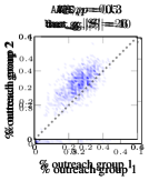
(d)

Figure 3: Joint outreach probability distribution for different datasets, different propagation probabilities $p$, and seedsets cardinalities $|S|$.

The impact of the conduction probability.

As a second experiment, we investigate the difference between mutual fairness and equity (difference in the expected value of the proportions), as a function of the conduction probability $p$. We consider the IV dataset as a case study and select seeds by using bas_g. We show our results in Fig. 4. Our mutual fairness metric shows a fundamentally different trend compared to the equity metric. Importantly, for $p\in(0,0.5)$, both metrics have an opposite trend: equity fairness increases to some extent meanwhile our metric suggests a huge fall in fairness in this region. For $p\in(0.5,0.7)$, there is a fall in equity fairness, while our fairness evaluation remains relatively constant. It is only for $p\in(0.8,1.0)$ that both metrics agree in trend. Thus, as in the previous experiment, the equity metric fails to adequately capture changes in fairness. For more experiments on other datasets, we refer to Section C.2.

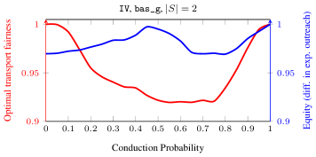
Figure 4: Optimal transport fairness (left axis, red) and equity (right axis, blue) calculated on IV dataset as $p$ varies in $[0,1]$.

3.3 Trading off Fairness and Efficiency

To construct our fairness metric, we completely discarded the efficiency of the final configuration. For instance, the “fairness distance” between a configuration whereby no agent receives the information (i.e., $\gamma=\delta_{(0,0)}$) and the “ideal” configuration whereby everyone receives the information (i.e., $\gamma^{\ast}$) is zero, as both probability distributions lay on the diagonal. As such, the fairness score of $\gamma=\delta_{(0,0)}$ is 1 and therefore maximal. Thus, in practice, one seeks a fairness-efficiency tradeoff.

In our setting, we can easily introduce the tradeoff in the transportation cost (2). Specifically, we can define the transportation cost as a weighted sum of the “diagonal distance” (measuring difference in efficiency, dotted segment in Fig. 2) and the “orthogonal distance” (measures difference in fairness, solid segment in Fig. 2). Formally, for a given weight $\beta\geq 0$, the arising transportation cost

$$c_{\beta}({\color[rgb]{0,0,1}(x_{1},x_{2})},{\color[rgb]{1,0,0}(y_{1},y_{2})}) =\beta\norm{{\color[rgb]{0,0.88,0}z(x_{1},x_{2},y_{1},y_{2})}-{\color[rgb]{0,0,1}(x_{1},x_{2})}}+(1-\beta)\norm{{\color[rgb]{0,0.88,0}z(x_{1},x_{2},y_{1},y_{2})}-{\color[rgb]{1,0,0}(y_{1},y_{2})}}$$

$$=\beta\absolutevalue{(x_{2}-x_{1})-(y_{1}-y_{2})}+(1-\beta)\absolutevalue{(x_{1}+x_{2})-(y_{1}+y_{2})}.$$ (3)

In particular, for $\beta=1$, we recover the transportation cost (2). We can then proceed as in Section 3.1. The “$\beta$-fairness-efficiency distance” between ${\color[rgb]{0,0,1}\gamma_{a}}$ and ${\color[rgb]{1,0,0}\gamma_{b}}$ is $W_{{c_{\beta}}}({\color[rgb]{0,0,1}\gamma_{a}},{\color[rgb]{1,0,0}\gamma_{b}})$ and the $\beta$-fairness metric can be then defined as follows.

Definition 3.2 ($\beta$-Fairness)

Consider a network with groups $C_{1},C_{2}$, a SIM algorithm is said to be $\beta$-fair if the algorithm propagation is such that it maximizes

$$\beta\mathrm{-}\textsc{Fairness}(\gamma)\coloneqq 1-\frac{1}{2-\beta}W_{{c_{\beta}}}(\gamma,\gamma^{\ast}),$$ (4)

with $W_{{c_{\beta}}}(\gamma,\gamma^{\ast})$ defined as in (1) with transportation cost as in (3.3) and ideal distribution $\gamma^{\ast}=\delta_{(1,1)}$.

The factors $1$ and and $1/(2-\beta)$ in (4) ensure that the metric is non-negative and in $[0,1]$. Again, the optimal transport problem can be solved in closed form, which yields

$$\beta\mathrm{-}\textsc{Fairness}(\gamma) =\mathbb{E}_{(x_{1},x_{2})\sim\gamma}\left[1-\frac{\beta\absolutevalue{x_{1}-x_{2}}+(1-\beta)\absolutevalue{x_{1}+x_{2}-2}}{2-\beta}\right]$$

In particular, for $\beta=1$, we recover the mutual fairness $\textsc{Fairness}(\gamma)$ in Definition 3.1 and for $\beta=0$ we obtain the efficiency metric $\mathbb{E}_{(x_{1},x_{2})\sim\gamma}[1-\frac{\absolutevalue{x_{1}+x_{2}-2}}{2}]$.

4 Improving Fairness

4.1 Fairness-promoting Seed-selection Algorithm

Armed with a novel fairness metric, we now design an iterative seed-selection algorithm, which we call Stochastic Seedset Selection Descent (S3D), that strategically selects seeds taking into account all communities simultaneously. The pseudo-code is summarized in Algorithm 1. For more details, we refer to Appendix D. For a given initial seedset, our algorithm explores new seeds and evaluates them on the efficiency-fairness metric $\beta\mathrm{-}\textsc{Fairness}$ as in (4) for a desired value of the fairness-efficiency tradeoff parameter $\beta$ (S3D_STEP() in Appendix D), to decide if the new seedset becomes a candidate for the optimized seedset. These seeds are searched for by iteratively sampling stochastically reachable nodes from the current seedset (SEEDSET_REACH() in Appendix D) while making sure they contribute to a non-overlapping outreach (Algorithm 1::5-7). To prevent getting stuck at some local minima of the generally non-convex objective, the procedure allows for visiting inferior seedsets on $\beta\mathrm{-}\textsc{Fairness}$ or even selecting completely random ones on rare occasions (Algorithm 1::12-18) using Metropolis Sampling [5]. Otherwise, a high $\beta\mathrm{-}\textsc{Fairness}$ encourages opting for the new seedset with high probability. Finally, we revisit all the seedset candidates collected so far and pick the one with the largest $\beta\mathrm{-}\textsc{Fairness}$ as the optimal seedset. For a sparse graph $G(V,E)$, with $E=O(V)$, choosing $|S|$ seeds, averaging over $R$ realizations to approximate outreach via Monte-Carlo sampling and exploring $k$ candidates using S3D_STEP suggests a total running time upper bound of $O(kR|S||V|)$ (see Appendix D for details about the algorithm complexity). In practice, $k\in[500,1000],R=1000$ for $S\in[2,100]$ works well for all datasets.

Input: Social Graph $G(V_{G},E_{G})$, initial seed set $S$, $\beta$ fairness weight, $\epsilon$-tolerance
Output: Optimal seedset $S^{*}$

1:$\mathcal{S}\leftarrow\{\}$ $\triangleright$ collection of candidates

2:for $k$ iterations do $\triangleright$ configurable $k$

3:     $V_{S}\leftarrow\text{nodes reachable from }$S via cascade, using seedset_reach routine

4:     $\hat{S}\leftarrow\{\}$

5:     for $|S|$ iterations do

6:         $\hat{S}\leftarrow\hat{S}\cup\{v\}\;|\;v\sim V_{S}$

7:         $V_{\hat{S}}\leftarrow\text{nodes reachable from }\hat{S}\text{ in a fixed horizon, using}$ seedset_reach

8:         $V_{S}\leftarrow V_{S}\setminus V_{\hat{S}}$      

9:     $E_{S}\leftarrow-\textsc{beta\_fairness}(S,\beta)$

10:     $E_{\hat{S}}\leftarrow-\textsc{beta\_fairness}(\hat{S},\beta)$

11:     $p_{\text{accept}}\leftarrow\min\{1,\mathrm{e}^{E_{S}-E_{\hat{S}}}\}$ $\triangleright$ $S$ acceptance based on energy change

12:     if $x\sim\mathcal{B}(p_{\text{accept}})$ then $\triangleright$ Metropolis Sampling in $12-18$

13:         $S^{+}\leftarrow\hat{S}$ $\triangleright$ get a better seedset

14:     else

15:         if $x\sim\mathcal{B}(\epsilon)$ then $\triangleright$ for some small constant $\epsilon$

16:              $S^{+}\leftarrow\{v_{i}\}_{i=1}^{|S|}\stackrel{{\scriptstyle|S|}}{{\sim}}V_{G}$ $\triangleright$ random seedset

17:         else

18:              $S^{+}\leftarrow S$ $\triangleright$ retain existing choice               

19:     $\mathcal{S}\leftarrow\mathcal{S}\cup\{S^{+}\}$

20:     $S\leftarrow S^{+}$ $\triangleright$ for next iteration

21:$S^{*}\leftarrow S\in\mathcal{S}\;|\;\textsc{beta\_fairness}(S,\beta)\text{ is maximum}$ $\triangleright$ via s3d_iterate

22:return $S^{*}$

Algorithm 1 Stochastic Seedset Selection Descent

4.2 Real-world Data

Are the outcomes more fair?

We test our algorithm across a variety of datasets (Appendix B) against our baselines (bas_d, bas_g). We initialize S3D algorithm with the two baseline seedsets and hence include results from two separately optimized seedsets, S3D_d, S3D_g. Our results are shown in Fig. 5. Informally, we observe that our seed-selection mechanism “moves” the probability mass of the joint outreach probability distribution towards the diagonal, which, ultimately, increases the fairness of the resulting configuration. At the same time, we either improve in efficiency as well or the sacrifice in efficiency is eventually minor, as we investigate more in detail in our next experiment. Generally speaking, datasets with high cross-group connections (AH, DZ, INS) can already benefit a lot from label-blind seed selection to get moderately fair outreach. Similarly, for datasets with low cross-group connections (APS) a label-blind strategy, in order to maximize efficiency, selects a diverse population of seeds from which all communities are reached. Therefore, label-blind algorithms work similarly to S3D. In other moderate cases (AV, HS, IV), instead, we observe significant improvements of S3D over label-blind strategies.

(a)

(b)

(c)

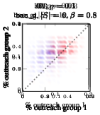
(d)

Figure 5: Demonstrate S3D (red) improvement over its label-blind baseline counter-part initializations (blue) for several datasets and propagation probabilities.Fig. 5(d) provides the strongest evidence that, besides improving in fairness, our strategy can also be more efficient, from $83.1\%$ to $87.9\%$.

Classification of seed-selection algorithms.

In our last experiments, we compare, across various datasets (Appendix B), several algorithms along with ours in terms of efficiency and mutual fairness. We consider the following algorithms: bas_d, bas_g, their fair heuristic counterparts, hrt_d, hrt_g, against our S3D_d, S3D_g, initialized via greedy and degree centrality baseline seeds, respectively. We show our results in Fig. 6. S3D achieves in almost all cases the highest fairness score ($y$-axis) and generally a slightly lower efficiency score ($x$-axis), compared to others. Thus, our seed-selection mechanism leads to fairer outcomes with only a minor decrease in efficiency.

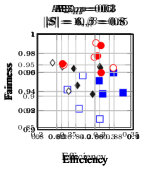
Figure 6: S3D trade-off and improvement against other label-aware and label-blind algorithms. Filled markers refer to greedy-based algorithms: $\blacksquare=$ bas_g, ● $=$ S3D_g, and $\blacklozenge=$ hrt_g. Empty markers refer to degree-based algorithms: $\square=$ bas_d, ○ $=$ S3D_d, and $\lozenge=$ hrt_d. For statistical bounds, we refer to Appendix E.

5 Conclusions and Limitations

Conclusions.

We propose a new fairness metric, called mutual fairness, in the context of SIM. Mutual fairness draws on optimal transport and captures various fairness-related aspects (e.g., when members of group 1 receive the information will members of group 2 receive it?) that are obscure to the fairness metrics in the literature. We also leverage our novel fairness metric to design a new seed selection strategy that tradeoffs fairness and efficiency. Across various real datasets, our algorithm yields superior fairness with a minor decrease (and in some cases even an increase) in efficiency.

Limitations.

Our proposed algorithm, S3D, is essentially a random combinatorial search in the graph defining the social network. As such, its performance will generally depend on the quality of the seedset initialization. Moreover, there is no guaranteed bound on the number of iterations needed in S3D to achieve a desired level of fairness. Both aspects can be limiting in real-world applications.

Appendix A Existing Fairness Metrics

Definition A.1 (Expected outreach ratio)

Given a network with communities $C_{1},\dots,C_{m}$, the SIM algorithm expected outreach ratio in $C_{i}$, $\bar{x}_{i}$, is the expected ratio of nodes reached in $C_{i}$, namely

$$\bar{x}_{i}:=\frac{\mathbb{E}[|v\text{ reached }|v\in C_{i}|]}{|C_{i}|},\quad\forall i\in\{1,\dots,m\}.$$

Definition A.2 (Equality [22])

Given the groups $C_{1},\dots,C_{m}$, a configuration is said to be equal, if the SIM algorithm chooses a seed set $S$ in a way such that the proportion of all communities in the seed set is the same, namely

$$\frac{\mathbb{E}[|v\in S|v\in C_{i}|]}{|C_{i}|}=\frac{\mathbb{E}[|v\in S|v\in C_{j}|]}{|C_{j}|}\quad\forall i,j\in\{1,\dots,m\}.$$

The notion of equality focuses on the fair allocation of seeds to the groups proportional to the size of the group within the population. This notion of fairness applies, for example, in the context of advertising companies that aim at having a fair distribution of resources among groups.

Definition A.3 (Equity [22])

Given a network with communities $C_{1},\dots,C_{m}$, a SIM algorithm that selects a seedset $S$ is said to be equitable if the algorithm propagation reaches all communities in a balanced way, i.e. $\bar{x}_{i}=\bar{x}_{j}$, $\forall i,j\in\{1,\dots,m\}$.

The notion of equity focuses on the outcome of the diffusion process, e.g. independent cascade, linear threshold model and it is suitable in contexts in which one aims to reach a diverse population in a calibrated way.

Definition A.4 (Max-min fairness [7])

Given the groups $C_{1},\dots,C_{m}$, the max-min fairness criterion maximizes the minimum expected outreach ratio among all groups, namely $\max\min_{i\in\{1,\dots,m\}}\bar{x}_{i}.$

The goal of the maxmin fairness is to minimize the gap among different groups in the outreach. The SIM problem under maxmin constraints has been investigated in [7, 8, 28].

Definition A.5 (Diversity [7])

Given the groups $C_{1},\dots,C_{m}$, let $k_{i}=\big{\lceil}k\cdot\frac{|C_{i}|}{|V|}\big{\rceil}$, where $k$ is the pre-specified total seed budget. Let $\bar{x}^{*}_{i}(C_{i}):=\max_{S\subset C_{i}:|S|=k_{i}}\bar{x}_{i}.$ A configuration is said to be diverse if for each $i\in\{1,\dots,m\}$ it holds $\bar{x}_{i}\geq\bar{x}^{*}_{i}(C_{i})$, where $\bar{x}_{i}$ refers to the expected outreach ratio in $C_{i}$ obtained from the seed set $S$, with $|S|=k$.

The notion of diversity ensures that each group receives influence at least equal to their internal spread of influence. The SIM problem under diversity constraints has been investigated in [7, 23].

Appendix B Description and Properties of Datasets

To associate the notion of fairness developed in Sections 3.1 and 3.3 with the datasets and the outcomes from experiments in Section 3.2 and 4.2, we summarize the dataset statistics in Table 1. Minority Frac. is calculated as the fraction of the minority group nodes in the entire population. Fraction of Cross Edges evaluates heterophily in the dataset, by calculating the fraction of edges that connect different groups. A higher value means a more heterophilic network, whereas a lower value means a more homophilic network.

Add Health (AH).

The Add Health datasets consists of a social network of students in schools and a relation between them is represented by whether they nominated each other in the Add Health surveys. We select a school at random with $1,997$ students and use race as the sensitive attribute (white and non-white).

Antelope Valley (AV),  [24].

We choose $4$ random networks among the $24$ available in the Antelope Valley dataset to compare our fairness improving algorithm, S3D, against [24], which worked on the same dataset. We also run our baselines and other fair seed selection heuristics from [22] on these datasets to get a fair comparison. The two sensitive attribute groups are male and female, self-reported in the dataset with binary attributes.

APS Physics (APS),  [14].

The APS citation network contains $1,281$ nodes, representing papers written in two main topics: Classical Statistical Mechanics (CSM), constituting $31.8\%$ of the papers, and Quantum Statistical Mechanics (QSM), accounting for the rest. As Lee et al. [14] analyze, the dataset has high homophily, meaning that each subfield cites more papers in their own field than in the other field. For simplicity, we use only the largest connected component in the full dataset (component stats in 1) between the two groups, for this study.

Deezer (DZ),  [19].

A social network from Europe with $18,442$ nodes, where each node has a self-reported attributed gender (male or female). Men are the minority ($44.3\%$) and women are the majority ($55.6\%$). The data has moderate homophily.

High School (HS),  [15].

A highschool friendship network collected from Mastrandrea et al. [15], with $133$ nodes in its main connected component represented by students who self-identify as male of female. The majority are female ($60\%$), and the network is homophilic.

Indian Villages (IV),  [1].

The dataset contains different demographic attributes for the individual networks and the household networks collected in $77$ Indian villages, from which we select Mothertongue (Telugu or Kannada) as the sensitive attribute. We note that most villages contain a majority mothertongue, either Telugu or Kannada. We pick a random village with $90$ individuals for our study.

Instagram (INS),  [21].

An interaction network from Instagram containing $553,628$ nodes, where everyone has a labeled gender ($45.57\%$ men and $54.43\%$ women). Each edge between two users represents a ‘like’ or ‘comment’ that one user gave another on a posted photo. The data has moderate homophily.

Dataset	$\#$ Nodes	$\#$ Edges	Avg. Degree	Diameter	Minority $\%$	Frac. Cross Edges
AH	1997	8523	8.54	10	34.6	0.452
AV_0	500	969	3.87	12	49	0.189
AV_2	500	954	3.81	14	49.6	0.183
AV_16	500	949	3.8	13	47.6	0.210
AV_20	500	959	3.84	15	48.4	0.198
APS	1281	3064	4.78	26	31.8	0.056
DZ	18442	46172	5.00	25	44.4	0.476
HS	133	401	6.03	10	40.6	0.394
IV	90	238	5.29	13	26.7	0.265
INS	553628	652830	2.36	16	45.6	0.417

Table 1: Summary statistics of Datasets used.

Appendix C Details on the Experiments and Extended Results

We use $R=1000$ throughout our experiments. For the outreach, we discretize the space $[0,1]\times[0,1]$ into $100\times 100$ equal sized bins. For S3D (refer to Appendix D), we use constants, exploit_to_explore$=1.3$, non_acceptance_retention_prob$=0.95$, and shallow_horizon$=4$.

C.1 Outreach Distribution

We report additional experiments in Figs. 7, 8, 9 and 10.

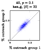
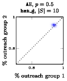
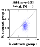
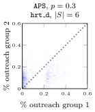
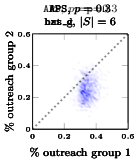
Figure 7: Outreach distribution.

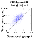
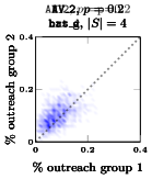
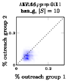
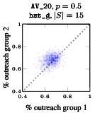
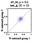
Figure 8: Outreach distribution.

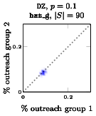
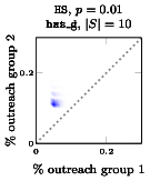
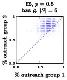
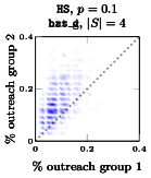
Figure 9: Outreach distribution.

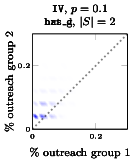
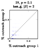
Figure 10: Outreach distribution.

C.2 The Impact of the Conduction Probability for Various Dataset

We report additional experiments in Figs. 11 and 12.

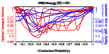
(a) bas_g seeds in AH, $|S|=6$

(b) bas_d seeds in APS, $|S|=15$

(c) bas_g seeds in APS, $|S|=15$

Figure 11: Part 1: Different definitions of fairness VS conduction probability on an outreach distribution created by the bas_g or bas_d heuristic.

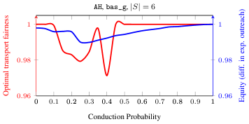
(a) bas_g seeds in AV_0, $|S|=20$

(b) bas_g seeds in DZ, $|S|=50$

(c) bas_g seeds in HS, $|S|=6$

(d) bas_g seeds in IV, $|S|=2$

Figure 12: Part 2: Different definitions of fairness VS conduction probability on an outreach distribution created by the bas_g heuristic.

C.3 Fairness-Efficiency performance of seedset selection algorithms

We report more experiments in Fig. 13.

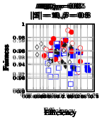
Figure 13: S3D trade-off and improvement against other label-aware and label-blind algorithms. Filled markers refer to greedy-based algorithms: $\blacksquare=$ bas_g, ● $=$ S3D_g, and $\blacklozenge=$ hrt_g. Empty markers refer to degree-based algorithms: $\square=$ bas_d, ○ $=$ S3D_d, and $\lozenge=$ hrt_d.

Appendix D Details on the Algorithm

D.1 Pseudocode

We provide more details on our algorithm, S3D, in two routines, Algorithm 2 and Algorithm 3.

Algorithm 2 Seed Selection Stochastic Descent (S3D) Step: Pseudo Code

1:function seedset_reach(seedset,G,p,horizon) $\triangleright$ nodes reached from seedset until horizon

2:     $\text{{realizations}}\leftarrow 1000$ $\triangleright$ for MCMC sampling, configurable

3:     $\text{{reach}}\leftarrow[]$

4:     while realizations do

5:         $\text{{reach}}\leftarrow\text{{reach}}+$ independent_cascade(seedset, G, p, horizon) $\triangleright$ collect nodes reached

6:         $\text{{realizations}}\leftarrow\text{{realizations}}-1$      

7:     return reach $\triangleright$ repetition of nodes reached

8:function s3d_step(seedset, G, p, fair_to_efficacy) $\triangleright$ each step delivers a new seedset

9:     $\text{{exploit\_to\_explore}}\leftarrow 1.3$ $\triangleright$ experimentally chosen, configurable

10:     $\text{{non\_acceptance\_retention\_prob}}\leftarrow 0.95$ $\triangleright$ prob. of retaining set

11:     $\text{{max\_horizon}}\leftarrow$ get_diam(G)

12:     $\text{{horizon\_factor}}\leftarrow$ $\text{{max\_horizon}}/4$ $\triangleright$ limit runtime

13:     $\text{{shallow\_horizon}}\leftarrow\text{{max\_horizon}}/\text{{horizon\_factor}}$

14:     $\text{{num\_seeds}}\leftarrow len(\text{{seedset}})$

15:     $\text{{seedset}}\leftarrow$ distinct(seedset)

16:     $\text{{seedset}}\leftarrow$ fit_to_size(seedset, num_seeds) $\triangleright$ fit to size with random nodes

17:     $\text{{reach}}\leftarrow\textsc{seedset\_reach}(\text{{seedset, G, p, max\_horizon}})$

18:     $\text{{candidate\_set}}\leftarrow[\textsc{sample}(\text{{reach}},1)]$ $\triangleright$ get first in candidate seedset

19:     while num_seeds do

20:         $\text{{last\_seed}}\leftarrow\text{{candidate\_set}}[-1]$ $\triangleright$ get latest seed

21:         $\triangleright$ remove shallow reach of last seed from current reach

22:         $\text{{reach}}\leftarrow\text{{reach}}-$ seedset_reach($[\text{{last\_seed}}]\text{{, G, p, shallow\_horizon}}$)

23:         $\text{{candidate\_set}}\leftarrow\text{{candidate\_set}}+[\textsc{sample}(\text{{reach}},1)]$ $\triangleright$ extend new seedset

24:         $\text{{num\_seeds}}\leftarrow\text{{num\_seeds}}-1$      

25:     $\text{{curr\_score}}\leftarrow$ -beta_fairness(seedset, fair_to_efficacy)

26:     $\text{{candidate\_score}}\leftarrow$ -beta_fairness(candidate_set, fair_to_efficacy)

27:     $\triangleright$ Metropolis Sampling

28:     $\text{{energy\_change}}\leftarrow\text{{curr\_score}}-\text{{candidate\_score}}$

29:     $\text{{accept\_prob}}\leftarrow$ clip($\text{{exp}}(\text{{exploit\_to\_explore}}*\text{{energy\_change}})$, $[0,1]$)

30:     $\text{{nonce\_1}}\leftarrow U(0,1)$

31:     if $\text{{nonce\_1}}<\text{{accept\_prob}}$ then

32:         return candidate_set $\triangleright$ get a better seedset

33:     else

34:         $\text{{nonce\_2}}\leftarrow U(0,1)$

35:         if $\text{{nonce\_2}}<\text{{non\_acceptance\_retention\_prob}}$ then

36:              return seedset $\triangleright$ retain existing choice

37:         else

38:              $\text{{random\_set}}\leftarrow$ sample(G.nodes, num_seeds)

39:              return random_set $\triangleright$ completely random selection rarely               

Algorithm 3 S3D Iteration: Pseudo Code

1:function s3d_iterate(seedset, G, p, fair_to_efficacy, num_iters)

2:     $\text{{least\_score\_seedset}}\leftarrow\text{{seedset}}$

3:     $\text{{least\_score}}\leftarrow$ -beta_fairness(seedset, fair_to_efficacy)

4:     while num_iters do

5:         $\text{{seedset}}\leftarrow$ s3d_step(seedset, G, p, fair_to_efficacy)

6:         $\text{{score}}\leftarrow$ -beta_fairness(seedset, fair_to_efficacy)

7:         if $\text{{score}}<\text{{least\_score}}$ then

8:              $\text{{least\_seedset}}\leftarrow\text{{seedset}}$          

9:         $\text{{num\_iters}}\leftarrow\text{{num\_iters}}-1$      

10:     return least_seedset

D.2 Estimating Runtime

We estimate the running time of Algorithm 2 and 3 combined. For the S3D_STEP, lines $9$-$13$ are constant operations and comprise dataset properties. Line $14,15$ cost $O(|S|)$. FIT_TO_SIZE can cost up to $O(|S|\log|V|)$ for sampling new $|S|$ nodes. SEEDSET_REACH does repeated BFS, and so costs $O(R(|V|+|E|))$. Lines $19$-$24$ cost as follows,

$$O((|S-1)(Rd_{\text{avg}}^{D_{\text{max}}}+R|V|+\log{R|V|})$$

where $d_{\text{avg}}$ is the average degree of the graph, and $D_{\text{max}}$ is the largest diameter of the graph. The first term here upper bounds the max computation in BFS for $D_{\text{max}}$ horizon. Other terms follow from the remaining operations in the while loop. Now, lines $25-26$ first create an outreach from the corresponding seedsets, costing $O(R(|V|+|E|))$ each, and then analytically calculate $\beta$-fairness for all the $R$ final configurations, costing $O(R*1)$ each. In the worst case, we might additionally execute lines $37-39$ costing $O(|S|\log|V|)$. So, a single S3D_STEP costs,

$$O(2|S|+|S|\log|V|+R(|V|+|E|) +(|S-1)(Rd_{\text{avg}}^{D_{\text{max}}}+R|V|+\log{R|V|})$$

$$+2(R(|V|+|E|)+R)+|S|\log|V|)$$

$$=O(|S|\log|V|+R(|V|+|E|)$$

$$+R|S|+R|S||V|+|S|\log|V|)$$

$$=O(|S|\log|V|+R|S||V|)$$

$$=O(R|S||V|).$$

Here, we used the assumption that $d_{\text{avg}}=O(2E/V)=O(1)$ for a sparse graph ($E=O(V)$). Now this S3D_STEP is run $k$ times using S3D_ITERATE to find the best seedset in these $k$ runs. Moreover, we avoid any redundant calculations and memoize $\beta$-fariness for any seedset we discover. Hence, the total runtime is $O(kR|S||V|)$, as claimed.

D.3 Illustrative Example

Consider the information spreading over the graph in Fig. 14 as an independent cascade model with probability $p=0.1$, with blue and red nodes belonging to two different groups. A greedy strategy would choose the seed set as $S_{g}={3,5}$ (enlarged nodes) as shown in Fig. 14(a), thus leading to the highly unfair outreach in Fig. 14(b). On the contrary, our algorithm S3D promotes the choice $S_{\texttt{S3D}}={1,4}$ reflected in 14(c), which gives the more fair outreach plotted in Fig. 14(d), showing that it improves over greedy/sophisticated label-blind seed selection strategies.

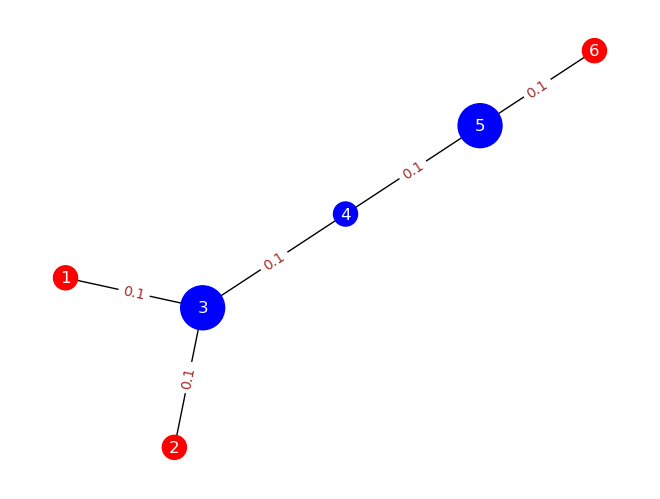
(a) Greedy Choice: Graph

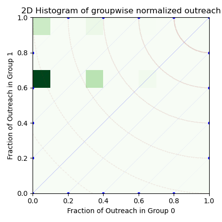
(b) Greedy Choice: Outreach

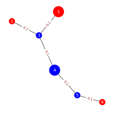
(c) S3D Choice: Graph

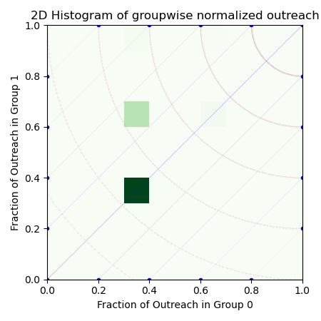
(d) S3D Choice: Outreach

Figure 14: Toy example to show label-aware choice using S3D over a label-blind seedset selection process. The enlarged nodes are selected seeds. Since the graph is small, the outreach discretization bucket have been granularized for improved readability.

Appendix E Error Bars on Fairness and Efficiency Experiments

Referring to Fig. 6, we mention $2$-sigma symmetrical error bars as follows.

-	Eff-Mean	Efficiency-Err-Bar ($\pm 2\sigma$)	Fair-Mean	Fairness-Err-Bar ($\pm 2\sigma$)
s3d_d	0.24	0.0022	0.94	0.002
hrt_d	0.105	0.005	0.911	0.004
bas_d	0.173	0.0016	0.803	0.003
s3d_g	0.25	0.002	0.945	0.002
hrt_g	0.17	0.0058	0.868	0.006
bas_g	0.318	0.002	0.898	0.003

Table 2: APS.

-	Eff-Mean	Efficiency-Err-Bar ($\pm 2\sigma$)	Fair-Mean	Fairness-Err-Bar ($\pm 2\sigma$)
s3d_d	0.241	0.005	0.95	0.002
hrt_d	0.227	0.005	0.951	0.002
bas_d	0.277	0.004	0.935	0.002
s3d_g	0.241	0.005	0.951	0.002
hrt_g	0.258	0.005	0.945	0.003
bas_g	0.3	0.004	0.926	0.003

Table 3: AV_0.

-	Eff-Mean	Efficiency-Err-Bar ($\pm 2\sigma$)	Fair-Mean	Fairness-Err-Bar ($\pm 2\sigma$)
s3d_d	0.08	0.0004	0.99	0.0008
hrt_d	0.08	0.0004	0.967	0.0007
bas_d	0.08	0.0004	0.91	0.001
s3d_g	0.08	0.0004	0.988	0.0008
hrt_g	0.08	0.0004	0.965	0.0008
bas_g	0.08	0.0004	0.938	0.0009

Table 4: HS, $p=0.01$.

-	Eff-Mean	Efficiency-Err-Bar ($\pm 2\sigma$)	Fair-Mean	Fairness-Err-Bar ($\pm 2\sigma$)
s3d_d	0.88	0.002	0.96	0.001
hrt_d	0.83	0.002	0.94	0.002
bas_d	0.83	0.002	0.94	0.002
s3d_g	0.87	0.002	0.96	0.002
hrt_g	0.86	0.002	0.935	0.002
bas_g	0.89	0.002	0.94	0.002

Table 5: HS, $p=0.5$.

Appendix F Declaration of Computational Resources

All experiments were performed on a local PC on a single CPU core $3.5$ GHz. Except for datasets DZ, INS, all datasets were loaded and operated on a local PC with $32$ GB of RAM. For the largest datasets (DZ, INS), we used remote compute clusters with $\sim 64$ GB memory and similar CPU capabilities. For the code development, we broadly used Python 3.10+, numpy, jupyter, and networkx [9]. Runtime for each non-S3D configured experiment on datasets except DZ, INS, was $10-15$ minutes. For DZ, INS, this was approximately $1-2$ hours. For S3D optimizations to be satisfactory, we ran each small dataset (except DZ, INS) for $1.5$ hours additionally. For massive datasets DZ, INS, the compute cluster took $\sim 4$ days for $k=10$ steps. The total set of experiments made, including the failed and passed or submitted ones, roughly took the same order of resources separately.

References

- Banerjee et al. [2013] Abhijit Banerjee, Arun G Chandrasekhar, Esther Duflo, and Matthew O Jackson. The diffusion of microfinance. Science, 341(6144):1236498, 2013.
- Black et al. [2020] Emily Black, Samuel Yeom, and Matt Fredrikson. Fliptest: fairness testing via optimal transport. Proceedings of the 2020 Conference on Fairness, Accountability, and Transparency (FAT’20), pages 111–121, 2020.
- Chen et al. [2012] Wei Chen, Wei Lu, and Ning Zhang. Time-critical influence maximization in social networks with time-delayed diffusion process. In Proceedings of AAAI Conference of Artificial Intelligence, 26(1):1–7, 2012.
- Chiappa et al. [2020] Silvia Chiappa, Ray Jiang, Tom Stepleton, Aldo Pacchiano, Heinrich Jiang, and John Aslanides. A general approach to fairness with optimal transport. Proceedings of the 2020 Conference on Fairness, Accountability, and Transparency (FAT’20), pages 3633–3640, 2020.
- Christian [2016] P. Robert Christian. The metropolis-hastings algorithm, 2016.
- Fangshuang et al. [2014] Tang Fangshuang, Qi Liu, Zhu Hengshu, Chen Enhong, and Feida Zhu. Diversified social influence maximization. 2014 IEEE/ACM International Conference on Advances in Social Networks Analysis and Mining (ASONAM 2014), pages 455–459, 2014.
- Farnadi et al. [2020] Golnoosh Farnadi, Behrouz Babaki, and Michel Gendreau. A unifying framework for fairness-aware influence maximization. International World Wide Web Conference 2020, pages 714–722, 2020.
- Fish et al. [2020] Benjamin Fish, Ashkan Bashardoust, Danah Boyd, Sorelle Friedler, Carlos Scheidegger, and Suresh Venkatasubramanian. Gaps in information access in social networks? International World Wide Web Conference 2019, San Francisco, USA, pages 480–490, 2020.
- Hagberg et al. [2008] Aric Hagberg, Pieter Swart, and Daniel Chult. Exploring network structure, dynamics, and function using networkx. 01 2008.
- Junaid et al. [2023] Ali Junaid, Babaei Mahmoudreza, Abhijnan Chakraborty, Baharan Mirzasoleiman, Krishna P. Gummadi, and Adish Singla. On the fairness of time-critical influence maximization in social network. IEEE Transaction on knowledge and data engineering, 35(3):480–490, 2023.
- Karimi et al. [2018] Fariba Karimi, Mathieu Génois, Claudia Wagner, Philipp Singer, and Markus Strohmaier. Homophily influences ranking of minorities in social networks. Scientific reports, 8(1):11077, 2018.
- Kempe et al. [2003] David Kempe, Jon Kleinberg, and Eva Tardos. Maximizing the spread of influence through a social network. Proceedings of the 9th ACM SIGKDD Conference on Knowledge Discovery and Data Mining, pages 137–146, 2003.
- Kempe et al. [2005] David Kempe, Jon Kleinberg, and Éva Tardos. Influential nodes in a diffusion model for social networks. In Automata, Languages and Programming: 32nd International Colloquium, ICALP 2005, Lisbon, Portugal, July 11-15, 2005. Proceedings 32, pages 1127–1138. Springer, 2005.
- Lee et al. [2019] Eun Lee, Fariba Karimi, Claudia Wagner, Hang-Hyun Jo, Markus Strohmaier, and Mirta Galesic. Homophily and minority-group size explain perception biases in social networks. Nature human behaviour, 3(10):1078–1087, 2019.
- Mastrandrea et al. [2015] Rossana Mastrandrea, Julie Fournet, and Alain Barrat. Contact patterns in a high school: a comparison between data collected using wearable sensors, contact diaries and friendship surveys. PloS one, 10(9):e0136497, 2015.
- Peyré et al. [2019] Gabriel Peyré, Marco Cuturi, et al. Computational optimal transport: With applications to data science. Foundations and Trends® in Machine Learning, 11(5-6):355–607, 2019.
- Rahmattalabi et al. [2021] Aida Rahmattalabi, Shahin Jabbari, Himabindu Lakkaraju, Phebe Vayanos, Max Izenberg, Ryan Brown, Eric Rice, and Milind Tambe. Fair influence maximization: A welfare optimization approach. In Proceedings of the AAAI Conference on Artificial Intelligence, volume 35, pages 11630–11638, 2021.
- Richardson and Domingos [2002] Matthew Richardson and Pedro Domingos. Mining knowledge-sharing sites for viral marketing. In Proceedings of 8th International Conference on Knowledge, Discovery and Data Mining, pages 61–70, 2002.
- Rozemberczki and Sarkar [2020] Benedek Rozemberczki and Rik Sarkar. Characteristic functions on graphs: Birds of a feather, from statistical descriptors to parametric models. In Proceedings of the 29th ACM international conference on information & knowledge management, pages 1325–1334, 2020.
- Si et al. [2021] Nian Si, Karthyek Murthy, Jose Blanchet, and Viet Anh Nguyen. Testing group fairness via optimal transport projections. Proceedings of the 38th International Conference on Machine Learning, pages 9649–9659, 2021.
- Stoica et al. [2018] Ana-Andreea Stoica, Christopher Riederer, and Augustin Chaintreau. Algorithmic glass ceiling in social networks: The effects of social recommendations on network diversity. In Proceedings of the 2018 World Wide Web Conference, pages 923–932, 2018.
- Stoica et al. [2020] Ana-Andreea Stoica, Jessy Xinyi Han, and Augustin Chaintreau. Seeding network influence in biased networks and the benefits of diversity. Proceedings of The Web Conference 2020, pages 2089–2098, 2020.
- [23] Alan Tsang, Bryan Wilder, Eric Rice, Milind Tambe, and Yair Zick. Group-fairness in influence maximization. Proceedings of the Twenty-Eighth International Joint Conference on Artificial Intelligence (IJCAI-19), pages 5997–6005.
- Tsang et al. [2019] Alan Tsang, Bryan Wilder, Eric Rice, Milind Tambe, and Yair Zick. Group-fairness in influence maximization. Proceedings of the Twenty-Eighth International Joint Conference on Artificial Intelligence (IJCAI-19), pages 5997–6005, 2019.
- Valente and Pumpuang [2007] Thomas W. Valente and Patchareeya Pumpuang. Identifying opinion leaders to promote behaviour change. Health, Education & Behaviour, 34(6):881–896, 2007.
- Villani [2009] Cédric Villani. Optimal transport: old and new, volume 338. Springer, 2009.
- Zehlike et al. [2022] Meike Zehlike, Alex Loosley, Håkan Jonsson, Emil Wiedemann, and Philipp Hacker. Beyond incompatibility: Trade-offs between mutually exclusive fairness criteria in machine learning and law. arXiv preprint arXiv:2212.00469, 2022.
- Zhu et al. [2019] Jianming Zhu, Smita Ghosh, and Weili Wu. Group influence maximization problem in social networks. IEEE Transactions on Computational Social Sciences, 6(6):1156–1164, 2019.