Can independent Metropolis beat crude Monte Carlo?

Abstract

Assume that we would like to estimate the expected value of a function $F$ with respect to a density $\pi$. We prove that if $\pi$ is close enough under KL divergence to another density $q$, an independent Metropolis sampler estimator that obtains samples from $\pi$ with proposal density $q$, enriched with a variance reduction computational strategy based on control variates, achieves smaller asymptotic variance than that of the crude Monte Carlo estimator. The control variates construction requires no extra computational effort but assumes that the expected value of $F$ under $q$ is analytically available. We illustrate this result by calculating the marginal likelihood in a linear regression model with prior-likelihood conflict and a non-conjugate prior. Furthermore, we propose an adaptive independent Metropolis algorithm that adapts the proposal density such that its KL divergence with the target is being reduced. We demonstrate its applicability in a Bayesian logistic and Gaussian process regression problems and we rigorously justify our asymptotic arguments under easily verifiable and essentially minimal conditions.

1 Introduction

1.1 The general problem

We address the following generic Monte Carlo estimation problem. We are given a probability density function $\pi$ on some state space $\mathbb{X}\subset{\mathbb{R}}^{d}$ which gives rise to a probability measure $\pi(\cdot)$ on $\mathbb{X}$. We want to estimate the expectation of a function $F:\mathbb{X}\rightarrow{\mathbb{R}}$ with respect to $\pi(\cdot)$ given by

$$\mathbb{E}_{\pi}[F]=\int_{\mathbb{X}}F(x)\pi(x)dx$$ (1)

and we assume that analytical integration of (1) is not feasible. The crude Monte Carlo estimation of this expectation simulates i.i.d. random variables $X_{1},X_{2},\ldots,X_{n}\sim\pi(\cdot)$ and then produces the unbiased estimator

$$\mu_{n,CMC}=\frac{1}{n}\sum_{i=1}^{n}F(X_{i})$$ (2)

with variance estimator $\sigma^{2}_{n,CMC}$ of order $O(1/n)$. The true variance of $F$ is thus given by

$$\sigma_{F}^{2}=n\sigma^{2}_{n,CMC}=\mathbb{E}_{\pi}[(F(x)-\mathbb{E}_{\pi}[F])^{2}].$$ (3)

In some challenging problems often met in Bayesian inference, high energy physics and rare event simulation in finance and insurance, the variance $\sigma^{2}_{n,CMC}$ is very large and variance reduction techniques are used to improve $\mu_{n,CMC}$, see for example Owen (2013). One such method is importance sampling, in which we sample i.i.d. $X_{1},X_{2},\ldots,X_{n}$ from some other probability density (importance function) $q^{*}$ on $\mathbb{X}$ with respect to a measure $q^{*}(\cdot)$ and then use the (biased) estimator

$$\mu_{n,IS}=\frac{\sum_{i=1}^{n}F(X_{i})w^{*}(X_{i})}{\sum_{i=1}^{n}w^{*}(X_{i})},~{}~{}w^{*}(X_{i})=\pi(X_{i})/q^{*}(X_{i})$$ (4)

which can achieve a variance smaller than $\sigma^{2}_{n,CMC}$ obtaining its smallest value when $q^{*}(x)\propto|F(x)-\mathbb{E}_{\pi}[F]|\pi(x)$ for all $x\in\mathbb{X}$, see Kahn and Marshall (1953). Another one is the use of control variates: if there exist functions (control variates) $\{U_{i}\}_{i=1}^{k}$ such that $E_{\pi}[U_{i}]$ are analytically available, then the estimator $\mu_{n,CMC}+\sum_{i=1}^{k}\beta_{i}(U_{i}-E_{\pi}[U_{i}])$ is unbiased and for appropriate values of the scalars $\beta_{i}$ has no larger variance than that of $\mu_{n,CMC}$.

In many problems, a good choice of an importance function $q^{*}(x)$ will not be available to estimate (1). This scenario is not rare when $\pi(\cdot)$ is high-dimensional, not only because it may be hard to both sample from $q^{*}(x)$ and mimic the shape of $|F(x)-\mathbb{E}_{\pi}[F]|\pi(x)$, but also because the variance of (4) might not exist when $q^{*}(x)$ has thinner tails than $F(x)\pi(x)$. The use of control variates $\{U_{i}\}_{i=1}^{k}$ might also be infeasible since when $\pi(x)$ is a non-standard density, analytical expressions for $\mathbb{E}_{\pi}[U_{i}]$ are rarely available. Motivated by this, we aim to introduce alternative Markov chain Monte Carlo (MCMC) estimators of (1), based on the independent Metropolis algorithm, that can have smaller asymptotic variance than $\sigma^{2}_{F}$. At the same time these estimators should be easy to use without requiring to compute intractable expectations $\mathbb{E}_{\pi}[U_{i}]$ of control variates under the target.

An independent Metropolis estimator can be derived by constructing a Markov chain on $\mathbb{X}$ which has $\pi(\cdot)$ as a stationary distribution by letting a density $q:\mathbb{X}\rightarrow{\mathbb{R}}$ be the transition function, or proposal density, of the chain. The dynamics of the independent Metropolis algorithm require to move from any state $x\in\mathbb{X}$ by proposing a new location $y\in\mathbb{X}$ from $q$ and accept it with probability

$$\alpha(x,y):=\begin{cases}\min\left(1,\frac{\pi(y)q(x)}{\pi(x)q(y)}\right),&\pi(x)q(y)>0,\\ 1,&\pi(x)q(y)=0.\end{cases}$$ (5)

By collecting, at stationarity, dependent samples $X_{1},X_{2},\ldots,X_{n}$ from the Markov chain, we construct the ergodic estimator

$$\mu_{n,IM}=\frac{1}{n}\sum_{i=1}^{n}F(X_{i})$$ (6)

which satisfies, under appropriate conditions (see section 2), a central limit theorem of the form

$$\sqrt{n}(\mu_{n,IM}-\mathbb{E}_{\pi}[F])=n^{-1/2}\sum_{i=1}^{n}(F(X_{i})-\mathbb{E}_{\pi}[F])\overset{D}{\to}N(0,\sigma^{2}_{IM})$$

with the asymptotic variance given by

$$\sigma^{2}_{IM}:=\lim_{n\to\infty}n\mathbb{E}_{\pi}\left[\left(\mu_{n,IM}-\mathbb{E}_{\pi}[F]\right)^{2}\right].$$ (7)

1.2 Outline of the basic methodology

At first sight the estimator $\mu_{n,IM}$ cannot compete with $\mu_{n,MC}$ because it is based on dependent samples and therefore we expect that its variance should be larger. Indeed $\sigma^{2}_{IM}=\sigma^{2}_{F}$ only when $q$ equals $\pi$. Our key idea is that we can exploit the Markovian structure of the MCMC samples to build, with negligible extra computational cost, new estimators with variance smaller than $\sigma^{2}_{n,CMC}$. We derive these new estimators based on approximate solutions to the Poisson equation of the Markov chain that allow the construction of control variates for $\mu_{n,IM}$. There are two requirements for these estimators to achieve smaller variance than $\mu_{n,CMC}$. The first is the ability to obtain analytically $\mathbb{E}_{q}[F]$ or $\mathbb{E}_{q}[{\tilde{F}}]$ for some function ${\tilde{F}}$ close to $F$. The second is that the proposal density $q$ is close to $\pi$. This is rigorously justified in our Theorem 2 which states that when $q$ is close enough to $\pi$ under KL-divergence, then the variance of the new estimator is smaller than $\sigma^{2}_{n,CMC}$. This gives a new perspective for Monte Carlo estimation of (1) using control variates that does not require the ability to obtain an importance density $q^{*}(x)$ close to $|F(x)-\mathbb{E}_{\pi}[F]|\pi(x)$ or to analytically evaluate $\mathbb{E}_{\pi}[U_{i}]$ for control variates $\{U_{i}\}_{i=1}^{k}$. Unlike importance sampling where the optimal $q^{*}$ depends on $F$ in our estimator the optimal $q$ depends only on $\pi$, and this implies that with no extra cost we can re-use the same MCMC samples to obtain variance reduction for many functions $F$.

In the first part of our work, we derive the new ergodic estimator for independent Metropolis algorithms for any real valued functions $F$ together with a theoretical result that proves that such estimator is a good generic candidate for estimating expectations $\mathbb{E}_{\pi}[F]$ if the proposal density $q$ is close enough to the target density. To illustrate the potential of this new estimator, we visit a challenging and popular problem in Bayesian statistics that refers to calculation of marginal densities of the form $\int F(x)\pi(x)dx$ where the likelihood $F(x)$ and prior $\pi(x)$ are non-conjugate and there is a likelihood-prior conflict. We show that our ergodic estimator can have significantly reduced variance compared to crude Monte Carlo. We further combine this estimator of the marginal likelihood with pseudo-marginal MCMC (Andrieu and Roberts, 2009) to sample over the model space without the need to obtain parameter estimates within each model.

In the second part, we build an adaptive independent Metropolis algorithm that updates every $B>1$ iterations the proposal density $q$ such that the KL-divergence $\mathbb{KL}(q(x)||\pi(x))$ is being reduced after every adaptation. This update is based on a recent strand of research that exploits stochastic gradient-based optimisation techniques for KL-divergence minimisation in variational inference (Ranganath et al., 2014) and adaptive MCMC (Gabrié et al., 2022). We provide rigorously justified asymptotic arguments for (i) ergodicity of the resulting Markov chain, (ii) convergence to distribution of the estimators, (iii) a weak law of large numbers when both $B$ and the MCMC sampling size go to infinity and (iv) convergence of the scalar estimators that are used to construct our control variates. These arguments show that our adaptive independent Metropolis algorithm, enriched with cost-free variance reduction ergodic estimator, can serve as a direct competitor to $\mu_{n,CMC}$ since it achieves smaller variance when $q$ approaches $\pi$ close enough, and can be a direct competitor to the importance sampling estimator $\mu_{n,IS}$ when a good proposal density $q^{*}$ is not available.

To experimentally evaluate the estimator based on the adaptive independent Metropolis scheme, we considered Bayesian inference problems in logistic regression and Gaussian process regression. For several functions of interest $F$, including non-linear functions of parameters such as the odds ratio, the variance reduction we achieved by adopting our estimator compared with the simple ergodic estimator of the adaptive independent Metropolis varied between $2.7$ and $54.5$.

1.3 Related work

There is a vast literature of variance reduction in MCMC via control variates; for a long list of references and some critical discussion see Alexopoulos et al. (2023). A strand of research is based on Assaraf and Caffarel (1999) who noticed that a Hamiltonian operator together with a trial function are sufficient to construct an estimator with zero asymptotic variance. They considered a Hamiltonian operator of Schrödinger-type that led to a series of zero-variance estimators studied by Valle and Leisen (2010), Mira et al. (2013), Papamarkou et al. (2014), Belomestny et al. (2020), South et al. (2023), Oates et al. (2017), Barp et al. (2022), South et al. (2022), Oates et al. (2019). Another approach which is closely related to our proposed methodology attempts to minimise the asymptotic variance of the ergodic estimator of the Markov chain. One way to achieve this is based on the observation that the solution of the Poisson equation for $F$ (also called the fundamental equation) automatically leads to a zero-variance estimator for $F$. Interestingly, a solution of this equation produces zero-variance estimators suggested by Assaraf and Caffarel (1999) for a specific choice of Hamiltonian operator. One of the rare examples that the Poisson equation has been solved exactly for discrete time Markov chains is the random scan Gibbs sampler where the target density is a multivariate Gaussian density and the goal is to estimate the mean of each components of the target density, see Dellaportas and Kontoyiannis (2012, 2009). Since direct solution of the Poisson equation is not available, approximate solutions have been suggested by Andradóttir et al. (1993), Atchadé and Perron (2005), Henderson (1997), Meyn (2008). Recently, Alexopoulos et al. (2023) provided a general framework that constructs estimators with reduced variance for random walk Metropolis and Metropolis-adjusted Langevin algorithms for means of each co-ordinate of a $d$-dimensional target density.

Adaptive Markov chain Monte Carlo algorithms with certain ergodic properties were proposed by Haario et al. (2001) and Roberts and Rosenthal (2009). An adaptation scheme of independent Metropolis together with its convergence properties is provided by Holden et al. (2009). Andrieu and Moulines (2006) and Roberts and Rosenthal (2007) studied the ergodicity properties of adaptive MCMC algorithms and provided central limit theorems and weak laws of large numbers. Recently, Gabrié et al. (2022) and Brofos et al. (2022) suggest applying adaptive MCMC by adopting normalizing flows as independent Metropolis proposal densities, which are optimised by KL-divergence minimisation using the history of states. In our adaptive MCMC algorithm we also use KL-divergence minimisation to optimise the proposal density $q$ but unlike Gabrié et al. (2022); Brofos et al. (2022) we make use of all candidate states (rejected or accepted) to adapt $q$. Specifically, we apply stochastic gradient methods based on the reprametrisation trick that are widely used for variational inference in machine learning (Titsias and Lázaro-Gredilla, 2014; Rezende et al., 2014; Kingma and Welling, 2013; Gianniotis et al., 2016; Kucukelbir et al., 2017; Salimans and Knowles, 2013; Tan and Nott, 2018).

Finally, a parallel path of research is based on adaptive importance sampling, see for example Richard and Zhang (2007); Cappé et al. (2008); Cornebise et al. (2008); Dellaportas and Tsionas (2019); Paananen et al. (2021). The goal is to target $q^{*}$ rather than $q$ and the adaptation process is somewhat different because it does not involve any Markov chain dynamics.

1.4 Outline of the paper

The rest of the paper is organised as follows. Section $2$ provides the methodological arguments and their rigorous justification for the construction of control variables for the ergodic estimator of the independent Metropolis algorithm together with illustrations with simulated and real data. Section $3$ deals with the construction of an adaptive independent Metropolis algorithm that adapts the proposal density such that its KL-divergence with the target is being reduced and illustrates its applicability with synthetic and real data. We conclude with a brief discussion in Section $4$.

2 Control variates for Independent Metropolis algorithms

2.1 A new estimator based on control variates

We denote by $IM(P,\pi,q)$ the independent Metropolis algorithm defined on the state space $\mathbb{X}\subset{\mathbb{R}}^{d}$ with transition kernel $P$ defined via (5) and two probability measures $\pi(\cdot)$ and $q(\cdot)$ with corresponding target and proposal densities $\pi(x)$ and $q(y)$. The transition kernel $P$ that generates the Markov chain based on $IM(P,\pi,q)$ is expressed by

$$P(x,dy):=\alpha(x,y)q(y)dy+\left(1-\int\alpha(x,z)q(z)dz\right)\delta_{x}(dy)$$

where $\delta_{x}$ is Dirac’s measure centred at $x$. Then, for any function $G:\mathbb{X}\rightarrow{\mathbb{R}}$ we have

$$PG(x) :=E_{x}[G(X_{1})]:=E_{x}[G(X_{1})|X_{0}=x]=\int P(x,dy)G(y)dy$$

$$=\int\alpha(x,y)q(y)G(y)dy+\left(1-\int\alpha(x,z)q(z)dz\right)G(x)$$

$$=G(x)+\int\alpha(x,y)(G(y)-G(x))q(y)dy.$$ (8)

Henderson (1997) observed that since the function $PG(x)-G(x)$ has zero expectation with respect to $\pi(\cdot)$, we can use it as control variate to reduce the variance of $\mu_{n,IM}$ by constructing, using (8), the control variate based estimator which is based on samples $X_{1},X_{2},\ldots,X_{n}$ and is given by

$$\mu_{n,IMCV,G}=\frac{1}{n}\sum_{i=1}^{n}\left\{F(X_{i})+\beta_{1}\int\alpha(X_{i},y)(G(y)-G(X_{i}))q(y)dy\right\}$$ (9)

for some scalar parameter $\beta_{1}$. Since $IM(P,\pi,q)$ is reversible, the optimal $\beta_{1}$ that minimises the asymptotic variance $\sigma^{2}_{IM}$ in (7) is given by

$$\beta^{\star}_{1}:=\frac{\mathbb{E}_{\pi}[(F-\mathbb{E}_{\pi}[F])(G+PG)]}{\mathbb{E}_{\pi}[G^{2}-(PG)^{2}]}$$ (10)

estimated by

$$\hat{\beta}_{1}=\frac{\sum_{i=1}^{n}F(X_{i})(G(X_{i})+PG(X_{i}))-n^{-1}\sum_{i=1}^{n}F(X_{i})\sum_{i=1}^{n}(G(X_{i})+PG(X_{i}))}{\sum_{i=2}^{n}(G(X_{i})-PG(X_{i-1}))^{2}};$$ (11)

see Theorem 3 of Dellaportas and Kontoyiannis (2012). The optimum choice of $G$ is the solution of Poisson equation $\hat{F}(x)$ for $F$:

$$\int\alpha(x,y)(\hat{F}(y)-\hat{F}(x))q(y)dy=-F(x)+\mathbb{E}_{\pi}[F],\text{ for every }x\sim\pi(\cdot),$$ (12)

that achieves zero variance for the estimator $\mu_{n,IMCV,{\hat{F}}}$ for any value of $n$ and for $\beta^{\star}_{1}=1$, see Dellaportas and Kontoyiannis (2012). Clearly the solution $\hat{F}(x)$ of (12) is translation invariant. Therefore, in the following we will denote by $\hat{F}(x)$ the any member of the class of all translations of $\hat{F}(x)$.

A research strategy that was used by Dellaportas and Kontoyiannis (2012) for random scan Gibbs samplers and by Alexopoulos et al. (2023) for random walk and Metropolis adjusted Langevin algorithms, is to find an estimator $\mu_{n,IMCV,G}$ based on some approximation $G\approx{\hat{F}}$. We follow the same research avenue for $IM(P,\pi,q)$ by first proving the following Theorem:

Theorem 1

(Proof in the Appendix A.1) Assume that for a target density $\pi(x)$ there exists a sequence of proposal distributions $\left\{q_{i}(x)\right\}_{i=1}^{\infty}$ such that $\lim_{i\rightarrow\infty}q_{i}(x)\rightarrow\pi(x)$ and for each proposal distribution $q_{i}$ the corresponding solution of the Poisson equation of $IM(P_{i},\pi,q_{i})$ for a function $F:\mathbb{X}\rightarrow{\mathbb{R}}$ is $\hat{F}_{i}(x)$. Then,

$$\lim_{i\rightarrow\infty}\hat{F}_{i}(x)\rightarrow F(x).$$

Theorem 1 guarantees that as the proposal density converges to the target density, the solution to the Poisson equation converges to the function $F$. It is straightforward to observe that at the limit $\lim_{i\rightarrow\infty}q_{i}(x)=\pi(x)$ the acceptance ratio $\alpha(x,y)$ in (12) becomes one and the solution of the Poisson equation is just ${\hat{F}}(x)=F(x)$. Motivated by this limiting case, for any independent Metropolis sampler (where $q(x)\neq\pi(x)$) we propose to use the function $G(x)=F(x)$ in the general control variate based estimator in (9), which leads to the estimator

$$\mu_{n,IMCV,F}=\frac{1}{n}\sum_{i=1}^{n}\left\{F(X_{i})+{\hat{\beta}}_{1}\int\alpha(X_{i},y)(F(y)-F(X_{i}))q(y)dy\right\}.$$ (13)

Unlike the approach of Alexopoulos et al. (2023), the above estimator does not require any approximation of function $G$ because it simply assumes that $G(x)=F(x)$ is a good approximation to ${\hat{F}(x)}$. However, (13) still requires the evaluation of the intractable integral $\int\alpha(X_{i},y)(F(y)-F(X_{i}))q(y)dy$ for each sampled point $X_{i}$. Since the transition kernel of the $IM(P,\pi,q)$ algorithm required one sample $Y_{i}\sim q$ every time the chain was at state $X_{i}$, a crude Monte Carlo estimator of this integral can be based on the (sample size one!) estimator $\alpha(X_{i},Y_{i})(F(Y_{i})-F(X_{i}))$, where all acceptance ratios $\alpha(X_{i},Y_{i})$ are available at no additional cost. This suggests that (13) can be approximated by

$$\mu_{n,IMCV,F}\approx\frac{1}{n}\sum_{i=1}^{n}\left\{F(X_{i})+{\hat{\beta}}_{1}\cdot\alpha(X_{i},Y_{i})(F(Y_{i})-F(X_{i}))\right\}.$$ (14)

A final trick to achieve our final estimator is to use a further control variate to reduce the variance of the estimator (14), by reducing the variance of the sample size one estimate $\alpha(X_{i},Y_{i})(F(Y_{i})-F(X_{i}))$ of the integral $\int\alpha(X_{i},y)(F(y)-F(X_{i}))q(y)dy$. If the expected value $\mathbb{E}_{q}[F]$ is analytically available then an immediate choice of control variate is the zero-mean random variable $F(Y)-\mathbb{E}_{q}[F]$ resulting to our proposed final estimator

$$\mu_{n,IMCV}=\frac{1}{n}\sum_{i=1}^{n}\left\{F(X_{i})+{\hat{\beta}}_{1}\left\{\alpha(X_{i},Y_{i})(F(Y_{i})-F(X_{i}))-{\hat{\beta}}_{2}(F(Y_{i})-\mathbb{E}_{q}[F])\right\}\right\}.$$ (15)

where $\hat{\beta}_{1}$ is calculated from (11) with $G=F$. Notice that $PF(x)$ depends on both the current value of the chain $X_{i}$ and the corresponding proposal value $Y_{i}$, so we will denote $PF(x)$ by $PF(x,y)=F(x)+\alpha(x,y)(F(y)-F(x))-{\hat{\beta}}_{2}(F(y)-\mathbb{E}_{q}[F])$ and we obtain

$$\hat{\beta}_{1}=\frac{\sum_{i=1}^{n}\{F(X_{i})(F(X_{i})+PF(X_{i},Y_{i}))\}-n^{-1}\sum_{i=1}^{n}F(X_{i})\sum_{i=1}^{n}(F(X_{i})+PF(X_{i},Y_{i}))}{\sum_{i=2}^{n}(F(X_{i})-PF(X_{i-1},Y_{i-1}))^{2}}.$$

The scalar ${\hat{\beta}}_{2}$ is the least squares estimator that minimises the asymptotic variance of the estimator

$$\frac{1}{n}\sum_{i=1}^{n}\left\{\alpha(X_{i},Y_{i})(F(Y_{i})-F(X_{i}))-{\hat{\beta}}_{2}(F(Y_{i})-\mathbb{E}_{q}[F])\right\}$$

so the optimal parameter is given by

$$\beta^{\star}_{2}:=\frac{Cov[\alpha(x,y)(F(y)-F(x)),(F(y)-\mathbb{E}_{q}[F])]}{Var[F(y)-\mathbb{E}_{q}[F]]}$$ (16)

estimated by

$$\hat{\beta}_{2}=\frac{\sum_{i=1}^{n}\alpha(X_{i},Y_{i})(F(Y_{i})-F(X_{i}))(F(Y_{i})-\mathbb{E}_{q}[F])}{\sum_{i=1}^{n}(F(Y_{i})-\mathbb{E}_{q}[F])^{2}};$$ (17)

see, for example, Owen (2013). Notice that when $q(x)=\pi(x)$, from (10) and (16) the regression coefficients are set to $\hat{\beta}_{1}=\hat{\beta}_{2}=1$ and the $IM(P,\pi,q)$ acceptance probability is $\alpha(X_{i},Y_{i})=1$, so we obtain the zero-variance estimator $\mu_{n,IMCV}=\mathbb{E}_{q}[F]=\mathbb{E}_{\pi}[F]$.

As a final note, we remark here that if the expected value $\mathbb{E}_{q}[F]$ is analytically intractable, but there exists an approximation ${\tilde{F}}$ of $F$ such that $\mathbb{E}_{q}{\tilde{F}}$ is analytically available, then we can replace the control variate $F(y)-\mathbb{E}_{q}[F]$ by the control variate ${\tilde{F}}(y)-\mathbb{E}_{q}{\tilde{F}}$ with corresponding replacements in estimators (15) and (17) given by

$$\mu_{n,IMCV,\tilde{F}}=\frac{1}{n}\sum_{i=1}^{n}\left\{F(X_{i})+{\hat{\beta}}_{1}^{\prime}\left[\alpha(X_{i},Y_{i})(F(Y_{i})-F(X_{i}))-{\hat{\beta}}_{2}^{\prime}\left({\tilde{F}}(Y)-\mathbb{E}_{q}{\tilde{F}}\right)\right]\right\}$$

where

$$\hat{\beta}_{1}^{\prime}=\frac{\sum_{i=1}^{n}\{F(X_{i})(F(X_{i})+PF(X_{i},Y_{i}))\}-n^{-1}\sum_{i=1}^{n}F(X_{i})\sum_{i=1}^{n}(F(X_{i})+PF(X_{i},Y_{i}))}{\sum_{i=2}^{n}(F(X_{i})-PF(X_{i-1},Y_{i-1}))^{2}},$$

$$PF(x,y)=F(x)+\alpha(x,y)(F(y)-F(x))-{\hat{\beta}}_{2}^{\prime}\left({\tilde{F}}(y)-\mathbb{E}_{q}{\tilde{F}}\right),$$

$$\hat{\beta}_{2}^{\prime}=\frac{\sum_{i=1}^{n}\alpha(X_{i},Y_{i})(F(Y_{i})-F(X_{i}))({\tilde{F}}(Y)-\mathbb{E}_{q}{\tilde{F}})}{\sum_{i=1}^{n}({\tilde{F}}(Y)-\mathbb{E}_{q}{\tilde{F}})^{2}}.$$

2.2 Connection to Rao–Blackwellisation by integrating out decision step

Another perspective of our proposed estimator is that it connects with and improves upon a basic Rao-Blackwellised estimator that integrates out the decision step at each Metropolis–Hastings iteration; see for instance Section 6.1 in Robert et al. (2018). Given that $X_{i}$ is the current state, $Y_{i}$ is the proposal and $u_{i}\sim U(0,1)$ is the uniform random variable to accept or reject $Y_{i}$, the IM estimator (or any other MCMC estimator) can be written as

$$\mu_{n,IM}=\frac{1}{n}\sum_{i=1}^{n}F(X_{i+1})=\frac{1}{n}\sum_{i=1}^{n}I(u_{i}<\alpha(X_{i},Y_{i}))F(Y_{i})+(1-I(u_{i}<\alpha(X_{i},Y_{i})))F(X_{i}),$$

where we used that the next state $X_{i+1}$ is equal to either $Y_{i}$ when the indicator function $I(u_{i}<\alpha(X_{i},Y_{i}))=1$ or $X_{i}$ otherwise. By taking the expectation under the uniform distribution $U(0,1)$ to integrate out $u_{i}$ we obtain

$$\frac{1}{n}\sum_{i=1}^{n}\alpha(X_{i},Y_{i})F(Y_{i})+(1-\alpha(X_{i},Y_{i}))F(X_{i})=\frac{1}{n}\sum_{i=1}^{n}\left\{F(X_{i})+\alpha(X_{i},Y_{i})(F(Y_{i})-F(X_{i}))\right\}$$

which is the same with (14) for $\hat{\beta}_{1}=1$. Therefore, an interpretation of our final proposed estimator $\mu_{n,IMCV}$ in (15) (when $\hat{\beta}=1$) is that it adds a control variate $F(Y_{i})-\mathbb{E}_{q}[F]$ to further reduce the variance associated with the proposed state $Y_{i}$ in the above Rao–Blackwellised estimator.

2.3 Theoretical justifications

The asymptotic variance of $\mu_{n,IMCV}$ is given by

$$\sigma^{2}_{IMCV}=\lim_{n\rightarrow\infty}Var_{\pi,q}[\sqrt{n}\mu_{n,IMCV}]$$ (18)

and the question that arises is when $\sigma^{2}_{IMCV}$ is smaller than $\sigma^{2}_{F}$. We define the space

$$L_{p}^{\pi,q}:=\left\{f(x)\Bigg{|}\int_{X}|f(x)|^{p}\pi(x)dx<\infty,\int_{X}|f(x)|^{p}q(x)dx<\infty\right\}$$

where $\pi$ and $q$ are the corresponding densities of $IM(P,\pi,q)$, and $w^{\star}:=\mathop{Sup}\limits_{x}(w_{x})$ where $w_{x}=\pi(x)/q(x)$. We state the following assumptions.

Assumption 1 (A1)

$F\in L_{4}^{\pi,q}$.

Assumption 2 (A2)

$w^{\star}<\infty$.

Assumption 3 (A3)

The Markov chain produced by the $IM(P,\pi,q)$ sampler is $\psi$-irreducible and aperiodic with unique invariant measure $\pi$, and there are functions $V:\mathbb{X}\rightarrow[0,\infty),W:\mathbb{X}\rightarrow[1,\infty)$, a small set $C\in\mathcal{B}$, and a finite constant $b$, such that the Lyapunov condition $PV-V\leq-W+b\mathbb{I}_{C}$ holds and $\pi(V^{2})\leq\infty$.

Assumptions (A1), (A2) and (A3), guarantee standard theoretical MCMC results as shown in the following proposition.

Proposition 1

(Proof in the Appendix A.2) Under (A1),(A2) and (A3):

1. $(LLN)$ $\mu_{n,IMCV}\rightarrow\mathbb{E}_{\pi}(F)$ as $n\rightarrow\infty\text{ }a.s.$

2. $(CLT)$ $\left\{\mu_{n,IMCV}-\mathbb{E}_{\pi}[\mu_{n,IMCV}]\right\}/\sqrt{n}$ converges in distribution to $N(0,\sigma^{2}_{IMCV})$ as $n\rightarrow\infty$

3. $\lim_{n\rightarrow\infty}({\hat{\beta}_{1n}},{\hat{\beta}_{2n})}\rightarrow(\beta^{\star}_{1},\beta^{\star}_{2})\text{ }a.s.$ where $\beta^{\star}_{1},\beta^{\star}_{2}=\arg\min_{({\hat{\beta}_{1n}},{\hat{\beta}_{2n}})}[\sigma^{2}_{IMCV}]$.

We now state our key result. By denoting the Kullback–Leibler(KL) divergence as

$$\mathbb{KL}(q_{\theta}(x)||\pi(x)):=\int q_{\theta}(x)\log\frac{q_{\theta}(x)}{\pi(x)}dx$$

we provide a general result that connects $\sigma^{2}_{IMCV}$ in (18) with $\sigma^{2}_{F}$ in (3) and $\sigma^{2}_{IM}$ in (7):

Theorem 2

(Proof in the Appendix A.3) Under (A1), (A2) and (A3), there exists a constant $\epsilon>0$ such that if $\mathbb{KL}(q_{\theta}(x)||\pi(x))\leq\epsilon$ then $\sigma^{2}_{IMCV}\leq\sigma^{2}_{F}\leq\sigma^{2}_{IM}$.

Theorem 2 states that under fairly general assumptions of the functions $F$ for which we need to calculate $\mathbb{E}_{\pi}[F]$, we can construct an $IM(P,\pi,q)$ sampler so that the ergodic estimator (15) achieves smaller variance of the corresponding crude Monte Carlo estimators (2) and the standard ergodic estimator of $IM(P,\pi,q)$ (6). This immediately suggests that a new methodological strategy to estimate $\mathbb{E}_{\pi}[F]$ with Monte Carlo is to use an $IM(P,\pi,q)$ sampler with a suitably chosen proposal density $q$ that has two properties: it approximates well $\pi$ and $\mathbb{E}_{q}[F]$ is analytically available. A plausible strategy is to approximate $\pi$ by mixture of normal or student-t densities which seems a much easier task than the standard importance sampling strategy which seeks to approximate $q^{*}(x)$ in (4) with mixture of densities that approximate $|F(x)-\mathbb{E}_{\pi}[F]|\pi(x)$; see, for example, Cappé et al. (2008). This strategy has another advantage when compared with importance sampling. When $q(x)$ is a mixture of normal or student-t densities, expectations of $\mathbb{E}_{q}(F)$ is available for many functions $F$. It is then straightforward to construct many estimators $\mu_{n,IMCV}$ for many functions $F$ using the same sample from the $IM(P,\pi,q)$ chain. This is in contrast with the importance sampling methods that require a new importance function $q^{*}(x)$ for every new function $F$. An example of such flexibility is shown in the logistic regression examples of Section 3.3.2 where reduced variance estimators based on the same MCMC sample are derived for the first two moments of the parameters and the posterior odds.

2.4 Numerical illustrations

In subsection 2.4.1 we illustrate Theorem 2 in simple synthetic data examples while in subsection 2.4.2 we consider a more challenging Bayesian model selection example. We examine the relative performance of our estimator $\mu_{n,IMCV}$ against the crude Monte Carlo estimator $\mu_{n,CMC}$. Our measure of performance is based on the variance reduction factor which is defined as the ratio of $\sigma^{2}_{F}/\sigma^{2}_{IMCV}$. In our experiments we fix $n$ and produce $T$ independent repetitions $\{\mu_{n,IMCV}^{(i)}\}_{i=1}^{T}$ and $\{\mu_{n,CMC}^{(i)}\}_{i=1}^{T}$ that are used to estimate a truncated version of the variance reduction factor by

$$VRF=\frac{\sum_{i=1}^{T}\{\mu_{n,CMC}^{(i)}-T^{-1}\sum_{i=1}^{T}\mu_{n,CMC}^{(i)}\}^{2}}{\sum_{i=1}^{T}\{\mu_{n,IMCV}^{(i)}-T^{-1}\sum_{i=1}^{T}\mu_{n,IMCV}^{(i)}\}^{2}}.$$ (19)

2.4.1 Synthetic data examples

We first construct a synthetic data example in which we assume that the target distribution $\pi(x)$ is a standard normal distribution $\mathcal{N}(x|0,1)$ and the quantity of interest is the expected value of $F(x)=x$. We choose two different proposals $q(y)$, a normal distribution $\mathcal{N}(y|0,\sigma^{2})$ and a zero-mean student-t distribution with $\nu$ degrees of freedom $t_{\nu}(y)$. Independent Metropolis algorithms were initialised when a point drawn from the proposal distribution is accepted. $T=20$ independent repetitions of size $n=5000$ samples were used to obtain the estimators $\{\mu_{n,IMCV}^{(i)}\}_{i=1}^{T}$ and $\{\mu_{n,CMC}^{(i)}\}_{i=1}^{T}$ that were used to construct the box-plots of Figures 1 and 1. It is evident that as the proposal densities approach the target, the sample variance of the estimators decreases. The corresponding VRFs are depicted (shown in log space) in Figures 1 and 1. Notice that when the proposal density is far away from the target, $\mu_{n,IMCV}$ has larger variance than that of $\mu_{n,CMC}$. Furthermore, Figures 1 and 1 depict the theoretical lower bounds for the variance reduction factor (19) which are used in the proof of Theorem 2 in Appendix A.3. For these particular examples these bounds can be analytically derived, see (• ‣ B.1) and (• ‣ B.1) in Appendix B.1.

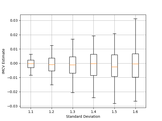
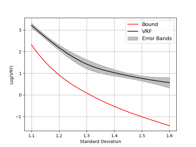
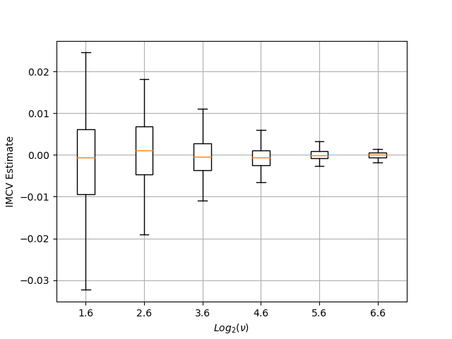
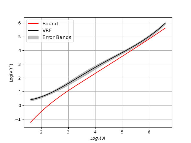
Figure 1: Comparison of $\mu_{n,IMCV}$ and $\mu_{n,CMC}$ estimators. Top row: $\mathcal{N}(x|0,1)$ target and $\mathcal{N}(x|0,\sigma^{2})$ proposal. Bottom row: $\mathcal{N}(x|0,1)$ target and $t_{\nu}(y)$ proposal. (a)-(c): Boxplots of $\mu_{n,IMCV}$ based on 20 repetitions for different values of $\sigma^{2}$ and $\nu$. (b)-(d): The logarithm of VRFs and corresponding theoretical bounds for different values of $\sigma^{2}$ and $\nu$.

2.4.2 Bayesian model selection in non-conjugate linear regression

We consider a standard linear regression $y=\boldsymbol{X}\beta+\epsilon$ where $y=(y_{1},y_{2},\ldots,y_{N})$ is a column vector of observations, $\boldsymbol{X}$ is an $N\times p$ design matrix, $\beta=(\beta_{1},\beta_{2},\ldots,\beta_{p})$ is a column vector of regression coefficients and $\epsilon$ is an error vector distributed as $\epsilon\sim N(0,\sigma^{2}\boldsymbol{I_{N}})$. The Bayesian approach to model selection requires the calculation of posterior model probabilities $f(m|y)\propto f(m)f(y|m)$ for all models $m$ specified by all $\beta_{m}$, the parameter vectors with elements the $2^{p}$ subsets of the set of $p$ elements of $\beta$, and the corresponding design matrices $\boldsymbol{X}_{m}$. In turn, this requires a specification of prior model probabilities $f(m)$ and the calculation of the marginal likelihood $f(y|m)$ of model $m$ which is given by

$$f(y|m)=\int f(y|m,\beta_{m})f(\beta_{m}|m)d\beta_{m}$$ (20)

where $f(y|m,\beta_{m})$ and $f(\beta_{m}|m)$ are the likelihood functions and parameter prior densities of model $m$. It is well-known that the choice of the prior $f(\beta_{m}|m)$ is of paramount importance in calculating posterior model probabilities and a careful specification is both necessary and an issue that has attracted a lot of interest in the literature; see, for example, Dellaportas et al. (2012). Perhaps the most popular and widely accepted default choice is the mixture of g-priors of Liang et al. (2008). An example of these priors that has been suggested by Liang et al. (2008) is given by

$$\beta_{m}|g,m\sim\mathcal{N}(0,g(\boldsymbol{X}_{m}^{\top}\boldsymbol{X}_{m})^{-1}),~{}~{}p(g)=(1+g)^{-2},~{}~{}g>0.$$ (21)

This and all other choices of mixtures of $g$-priors result in making integration of (20) intractable. This is a typical situation in Bayesian model choice literature where huge efforts have been made to propose ways to approximate such intractable marginal likelihoods.

It has often been noted (see for example Newton and Raftery (1994)) that an obvious solution would be to adopt a crude Monte Carlo estimator by sampling from the prior and estimating (20) as the expected likelihood function. However, since the posterior is often concentrated relative to the prior, Monte Carlo estimators will be very inefficient; see McCulloch and Rossi (1992) for a discussion. Although many strategies for increasing the efficiency of the crude Monte Carlo are available, it seems that there is nothing available to aid the estimation of the marginal likelihood of a linear regression model with the possibly most popular default prior density. Note that we cannot, at least readily, find functions of $\beta_{m}$ such that their analytical expectations with respect to the prior (21) are available, so is not easy to construct control variables to reduce the variance of the crude Monte Carlo estimator.

We test our $\mu_{n,IMCV}$ estimator by estimating (20) in synthetic data where there is a clear prior-posterior conflict. We generate $N=50$ data points with predictors $X_{i}\sim\mathcal{N}(0,1)$, $i=1,\ldots,4$ and response $Y\sim\mathcal{N}(4X_{3}+4X_{4},2.5^{2})$. The $IM(P,\pi,q)$ algorithm with $\pi$ being the prior (21) requires a proposal density $q$. Our estimator $\mu_{n,IMCV}$ performs well when this proposal is both close to the target density (21) and the expectation $\mathbb{E}_{q}[f(y|m,\beta_{m})]$ is analytically available. We choose to use a proposal of the form

$$q(\beta_{m})=\sum_{i=1}^{K}w_{i}\mathcal{N}(\beta_{m}|0,g_{i}(\boldsymbol{X}_{m}^{\top}\boldsymbol{X}_{m})^{-1}),\text{ such that }\sum_{i=1}^{K}w_{i}=1,~{}0<w_{i}<1.$$ (22)

For fixed $K$ and model $m$ the parameters $\left\{w_{i},g_{i}\right\}_{i=1}^{K}$ can be estimated by an Expectation-Maximisation(EM) algorithm as follows. Let $\boldsymbol{I}_{(m)}$ be an identity matrix with dimension equal to the dimension of $\beta_{m}$. We fit a $\sum_{i=1}^{K}w_{i}\mathcal{N}(0,g_{i}\boldsymbol{I}_{(m)})$ model based on 1000 data points generated from the generic prior

$$\beta_{m}|g,m\sim\mathcal{N}(0,g\boldsymbol{I}_{(m)}),~{}~{}p(g)=(1+g)^{-2},~{}~{}g>0$$ (23)

and we obtain estimates ${\hat{w}}_{i}$ and ${\hat{g}}_{i}$. Note that this algorithm is fitted only once and converges rapidly because all normal components have zero means. Then we sample $\beta^{{}^{\prime}}$ from the density

$$q(\beta^{\prime})=\sum_{i=1}^{K}{\hat{w}}_{i}\mathcal{N}(\beta^{{}^{\prime}}|0,{\hat{g}}_{i}\boldsymbol{I}_{(m)})$$ (24)

and we exploit the invariance of the KL divergence under linear transformation to obtain $\beta_{m}=(\boldsymbol{X}_{m}^{\top}\boldsymbol{X}_{m})^{-\frac{1}{2}}\beta^{{}^{\prime}}$ as samples generated from the density (22) that matches very well (21).

We chose $K=4$ by visual inspecting a Q-Q plot of the samples of (23) and (24). The $IM(P,\pi,q)$ algorithm ran for $1000$ iterations and compared with the corresponding crude Monte Carlo through VRFs based on $100$ independent repetitions of the experiment. Results for all $15$ models are shown in Table 1 where it is evident that our estimator approximates well the marginal likelihood in all models. For comparative purposes we have included precise estimations of the marginal likelihoods obtained by first integrating $\beta_{m}$ and then performing numerical integration over $g$. Notice that the difference of marginal likelihoods in $\log_{10}$-scale is used in Kass and Raftery (1995) as a way to interpret the weighted evidence against a null hypothesis with Bayes factors. It is also clear that as the parameter dimension increases, the variance of the crude Monte Carlo estimator and consequently the size of the variance reduction factor increase.

A realistic application of Bayesian model choice is when the size of models under comparison is large so estimation of all marginal likelihoods (20) is not feasible. In these cases model search MCMC algorithms that sample in the space of models provide a way to calculate posterior model probabilities only in models $m$ in which $f(m|y)$ is not negligible; see, for example Liang et al. (2022). However, this typically requires the analytical availability of the marginal likelihood (20) for each model $m$. Our unbiased independent Metropolis estimator of the marginal likelihood allows the bypass of this requirement by using a model search algorithm which is based on the pseudo-marginal MCMC proposed by Andrieu and Roberts (2009) and simply uses as target mass function our estimators of (20) for each model $m$. For illustration, we performed a simple random walk MCMC algorithm on the discrete space of the $15$ models in our example and in Figure 2 it is shown that the pseudo-marginal MCMC based on our estimators performs very well and certainly much better than the corresponding crude Monte Carlo based algorithm. The precise estimates of Table 1 based on numerical integration are also shown.

Table 1: Marginal Likelihood estimation for different models $X_{m}$ where $m$ is specified by which covariates are in the model. Results are reported as negative log-estimates and compared with a numerical integration estimation. VRF denotes the variance reduction factor.

Model	-$\log_{10}(\mu_{1000,IMCV})$	-$\log_{10}(\mu_{1000,CMC})$	Numerical integration	VRF
$X_{1}$	93.19	93.19	93.19	4.29
$X_{2}$	93.77	93.77	93.77	3.74
$X_{3}$	77.23	77.08	77.16	8.71
$X_{4}$	72.78	72.80	72.77	6.30
$X_{12}$	93.35	93.34	93.35	5.01
$X_{13}$	77.95	77.81	77.94	8.10
$X_{14}$	73.52	73.66	73.51	4.02
$X_{23}$	77.82	77.66	77.83	5.39
$X_{24}$	73.57	73.36	73.55	16.74
$X_{34}$	55.31	55.08	55.29	37.25
$X_{123}$	78.53	78.30	78.53	30.34
$X_{124}$	74.20	73.97	74.23	25.36
$X_{134}$	55.39	55.49	55.34	49.12
$X_{234}$	56.14	55.56	56.00	106.15
$X_{1234}$	55.91	57.71	55.93	4763.42

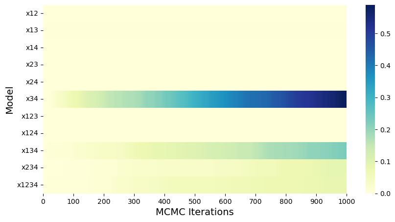
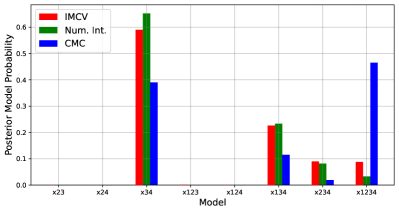
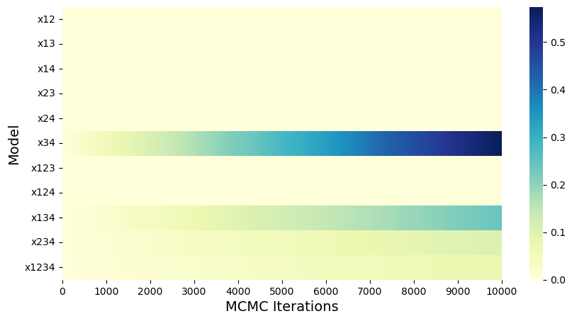
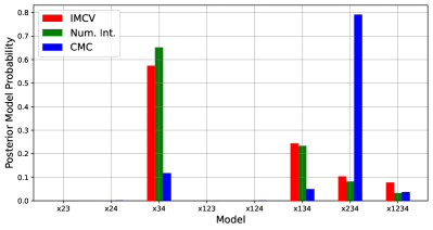
Figure 2: Comparison of $\mu_{n,IMCV}$ and $\mu_{n,CMC}$ estimators in pseudo-marginal MCMC. Top row: 1000 MCMC runs and 100 samples for pseudo-marginal likelihood estimates. Bottom row: 10000 MCMC runs and 10 samples for pseudo-marginal likelihood estimates. (a)-(c): Heatmap of the posterior probability mass function with $\mu_{n,IMCV}$ estimators. (b)-(d): Comparison of converged probability mass functions of the posterior model probability mass functions under different estimators. IMCV: Independent Metropolis with control variates; Num. Int.: Precise estimates with numerical integration; CMC: Crude Monte Carlo.

3 Adaptive independent Metropolis

In general, we consider the sequence of independent Metropolis adaptations $\{IM(P_{i},\pi,q_{\theta_{i}})\}_{i=1}^{\infty}$ identified by the proposal densities $\{q_{\theta_{i}}\}_{i=1}^{\infty}$, indexed by corresponding parameter vectors $\theta_{i}\in\Theta$. For each step $i$, we have an update function $H_{\theta_{i}}(x)$ and its stepsize $\alpha_{i}$. Then, the adaptive independent Metropolis can be implemented as shown in Algorithm 1.

Algorithm 1 General adaptive independent Metropolis

Input: Parameterised proposal distribution $q_{\theta}$, (intractable) target distribution $\pi$, update function $H_{\theta}(x)$, stepsize $\alpha$, total number of adaptation iterations $T$.
Initialisation Set $i\leftarrow 0$ and initialise {$X$, $q_{\theta}$, $H_{\theta}(x)$, $\alpha$} by {$X_{0}$, $q_{\theta_{0}}$, $H_{\theta_{0}}(X_{0})$, $\alpha_{0}$}.

1:while $i\leq T$ do

2:     Save sample $(X_{i},Y_{i})$ from independent Metropolis $IM(P_{i},\pi,q_{\theta_{i}})$.

3:     Adaptation update $\theta_{i+1}\leftarrow\theta_{i}-\alpha_{i}H_{\theta_{i}}(Y_{i})$.

4:     Set $i\leftarrow i+1$.

5:end while

Return: Proposals and samples $\{q_{\theta_{i}},X_{i},Y_{i}\}_{i=1}^{T}$.

The ergodicity of the Markov chain is guaranteed by assumptions on the specific procedure of adaptation. Throughout this Section we will be assuming that all independent Metrpolis sampling chains have a state space $\mathbb{X}$ and satisfy the following Assumption:

Assumption 4 (A4)

The parameters of the proposal density converge through the long run of Algorithm 1, i.e. $\lim_{i\rightarrow\infty}\theta_{i}=\theta^{\star}$, for some $\theta^{\star}\in\Theta$.

Moreover, in order to explore the properties of the adaptive MCMC, we need to rewrite (A2) and (A3) into their adaptation version:

Assumption 5 (A5)

$w^{\star}<\infty$ for all $q_{\theta}$ with $\theta\in\Theta$.

Assumption 6 (A6)

The Markov chain produced by the $IM(P_{i},\pi,q_{\theta_{i}})$ sampler is $\psi$-irreducible and aperiodic with unique invariante measure $\pi$ for all $i=1,2,\ldots$, and there are functions $V:\mathbb{X}\rightarrow[0,\infty),W:\mathbb{X}\rightarrow[1,\infty)$, a small set $C\in\mathcal{B}$, and a finite constant $b$, such that the Lyapunov condition $P_{i}V-V\leq-W+b\mathbb{I}_{C}$ holds and $\pi(V^{2})\leq\infty$.

3.1 Adaptation based on KL divergence

Theorem 2 and the numerical illustrations of the previous Section indicate that the key element of a good estimator of an $IM(P,\pi,q)$ sampler is the ability to obtain a good proposal density $q$ that is as close as possible, in terms of KL divergence, to the target $\pi$. Therefore, in this Section we define the update function $H_{\theta}$ in Algorithm 1 as a gradient direction towards minimising the KL divergence $\mathbb{KL}(q_{\theta}(x)||\pi(x))$. To further justify this choice, we present the following result from Theorem 2.

Corollary 1

(Proof in the Appendix A.4) Suppose there exists a sequence of constants $\{\epsilon_{i}\}_{i=1}^{\infty}$ and a sequence of proposals $\{q_{\theta_{i}}\}_{i=1}^{\infty}$ such that $\mathbb{KL}(q_{\theta_{i}}(x)||\pi(x))\leq\epsilon_{i}$ for every $i$, and $\lim_{i\rightarrow\infty}\epsilon_{i}=0$. Under (A1), (A5) and (A6) , define $\sigma^{2}_{IMCV,(i)}$ to be the asymptotic variance of (15) with $IM(P_{i},\pi,q_{\theta_{i}})$ sampler, then

$$\lim_{i\rightarrow\infty}\sigma^{2}_{IMCV,(i)}=0.$$

Corollary 1 indicates that if we obtain a sequence of adaptations $\{IM(P_{i},\pi,q_{\theta_{i}})\}_{i=1}^{\infty}$ such that the proposal densities approach the target density as $i$ increases, we can achieve zero variance estimators. The requirement is the adaptation to satisfy

$$\mathbb{KL}(q_{\theta_{i}}(x)||\pi(x))=\int q_{\theta_{i}}(x)\log\frac{q_{\theta_{i}}(x)}{\pi(x)}dx\leq\epsilon_{i}$$

for a sequence of $\{\epsilon_{i}\}_{i=1}^{\infty}$ that converges to zero.

In practice, a way to obtain the sequence of the adapted proposal distributions $q_{\theta_{i}}$ is by applying gradient descent updates on the parameters in order to minimise the above KL divergence. The gradient descent update takes the form

$$\theta_{i+1}=\theta_{i}-\alpha_{i}\nabla_{\theta_{i}}\mathbb{KL}(q_{\theta_{i}}(x)||\pi(x)),\ \text{where }\nabla_{\theta_{i}}\mathbb{E}(q_{\theta_{i}}||\pi)=\nabla_{\theta_{i}}\mathbb{E}_{q_{\theta_{i}}}\log\frac{q_{\theta_{i}}(x)}{\pi(x)}$$ (25)

and $\alpha_{i}>0$ is a step size parameter. This exact optimisation procedure is not feasible since the gradient is not available in closed-form, and instead we can apply stochastic optimisation (Robbins and Monro, 1951) where we use unbiased estimates of the gradients. More precisely, we can follow the recent literature in machine learning where such stochastic gradient optimisation methods are widely used for KL-based variational inference (Ranganath et al., 2014; Titsias and Lázaro-Gredilla, 2014; Kingma and Welling, 2013; Kucukelbir et al., 2017). We will assume that the independent Metropolis proposal $q_{\theta}(x)$ is reparametrisable from a simpler distribution $p(z)$, which enables the use of efficient reparametrisation gradient methods (Titsias and Lázaro-Gredilla, 2014; Rezende et al., 2014; Kingma and Welling, 2013; Gianniotis et al., 2016; Salimans and Knowles, 2013; Tan and Nott, 2018). For instance, for the standard multivariate Gaussian proposal $q_{\theta}(x)=\mathcal{N}(\mu,\boldsymbol{\Sigma})=\mathcal{N}(\mu,\boldsymbol{L}\boldsymbol{L}^{\top})$ where $\theta=(\mu,\boldsymbol{L})$ and $\boldsymbol{L}$ is the Cholesky factor of the covariance matrix, we can reparametrise $x\sim\mathcal{N}(\mu,\boldsymbol{L}\boldsymbol{L}^{\top})$ as $\mu+\boldsymbol{L}z,z\sim\mathcal{N}(0,\boldsymbol{I}_{d})$, and then consider as the update function $H_{\theta}(Y)$ in Algorithm 1 the unbiased gradient

$$H_{\theta}(Y)=\nabla_{\theta}\mathbb{E}_{q_{\theta}(x)}[\log q_{\theta}(x)]-\nabla_{\theta}\log\pi(Y=\mu+\boldsymbol{L}z),\ \ z\sim\mathcal{N}(0,\boldsymbol{I}_{d}),$$ (26)

where $\mathbb{E}_{q_{\theta}(x)}[\log q_{\theta}(x)]$ is the negative entropy of the Gaussian distribution; see Appendix D. The simplest form of adaptation is to apply stochastic optimisation updates at each iteration of independent Metropolis, i.e. similarly to standard adaptive MCMC (Haario et al., 2001; Roberts and Rosenthal, 2009; Andrieu and Thoms, 2008). To perform the adaptation step at the $i$-th sampling iteration we use the proposed state $Y_{i}=\mu_{i}+\boldsymbol{L}_{i}z_{i}\sim q_{\theta_{i}}$ to evaluate the unbiased gradient in (26), and then perform a gradient step to obtain the new parameters $\theta_{i+1}$ by applying the update step in Algorithm 1 (line 3).

Further implementation details of the above unbiased gradient estimation procedure towards minimising the KL divergence are given in Appendix D and Algorithm 3.

3.2 Theory and implementation of the adaptive independent Metropolis

3.2.1 Sample collection after adaptation

A trivial sub-optimal way to implement the general adaptation Algorithm 1 is to adapt $q_{\theta}$ until it reaches a final proposal density $q_{\theta_{T}}$ and ignore the samples generated by the adaptations $\{IM(P_{i},\pi,q_{\theta_{i}})\}_{i=1}^{T-1}$. Then, the ergodic estimator (15) can be evaluated by using the samples from the non-adaptive algorithm $IM(P_{T},\pi,q_{\theta_{T}})$ and the Proposition 1 provides the necessary theoretical guarantees for such scheme.

3.2.2 Sample collection during adaptation

Clearly the previous sampling scheme of subsection 3.2.1 can be inefficient since it produces an estimator that ignores all samples from the adaptation phase. In this section, we wish to construct better estimators that make use of all samples, and to that end we will study the properties of the whole sequence of the independent Metropolis adaptations $\{IM(P_{i},\pi,q_{\theta_{i}})\}_{i=1}^{\infty}$ and the corresponding sequence of generated samples.

Laws of large numbers (LLN) and central limit theorems (CLT) have been proved for various cases of $\{IM(P_{i},\pi,q_{\theta_{i}})\}_{i=1}^{\infty}$ sequences, see Andrieu and Moulines (2006) and Roberts and Rosenthal (2007). However, some of the conditions required for these proofs are hard to verify in practice, see for example Andrieu and Moulines (2006). Roberts and Rosenthal (2007) prove a LLN that assumes that the function $F$ is bounded. We propose an adaptive $\{IM(P_{i},\pi,q_{\theta_{i}})\}_{i=1}^{\infty}$ algorithm in which adaptation takes place every $B$ iterations. This has two key advantanges. First, the update (25) is based on $B$ samples so the estimate (26) is based on $B$ samplers. Second, our estimator is now based on $\ell$ batches of size $B$, $n=\ell B$, and this allows us to prove a LLN relaxing the assumption of boundness of $F$.

Assume that we collect samples $\left\{\left\{(X_{ij},Y_{ij})\right\}_{j=1}^{B}\right\}_{i=1}^{\ell}$ where $X_{ij}$ denote the accepted samples and $Y_{ij}$ denote the corresponding proposal values from the proposal densities $\{q_{\theta_{i}}\}_{i=1}^{\ell}$. Our estimator is

with

$$\hat{\beta}_{1i}=\frac{\sum_{j=1}^{B}\{F(X_{ij})(F(X_{ij})+PF(X_{ij},Y_{ij}))\}-\frac{1}{B}\sum_{j=1}^{B}\{F(X_{ij})\}\sum_{j=1}^{B}\{F(X_{ij})+PF(X_{ij},Y_{ij})\}}{\sum_{j=2}^{B}\{F(X_{ij})-PF(x_{i(j-1)})\}^{2}}$$ (28)

and

$$\hat{\beta}_{2i}=\frac{\sum_{j=1}^{B}\alpha(X_{ij},Y_{ij})(F(Y_{ij})-F(X_{ij}))(F(Y_{ij})-\mathbb{E}_{q_{\theta_{i}}}[F])}{\sum_{j=1}^{B}(F(Y_{ij})-\mathbb{E}_{q_{\theta_{i}}}[F])^{2}}.$$ (29)

Algorithm 2 Batch Adaptive Independent Metropolis with control variate

Inputs: Parameterised proposal distribution $q_{\theta}$, (intractable) target distribution $\pi$, update function $H_{\theta}(x)$, stepsize $\alpha$, batch size $B$, the number of batches $\ell$, objective function $F$.
Initialisation Set $i\leftarrow 0,j\leftarrow 0$ and initialise {$X$, $q_{\theta}$, $H_{\theta}(x)$, $\alpha$} by {$X_{0}$, $q_{\theta_{0}}$, $H_{\theta_{0}}(X_{0})$, $\alpha_{0}$}.

1:while $i<\ell$ do

2:     while $j<B$ do

3:         Save $\{\alpha(X_{ij},Y_{ij}),X_{ij},Y_{ij}\}$ from independent Metropolis $IM(P_{i},\pi,q_{\theta_{i}})$.

4:         Set $j\leftarrow j+1$.

5:     end while

6:     Adaptation update $\theta_{i+1}\leftarrow\theta_{i}-\alpha_{i}\sum_{j=1}^{B}H_{\theta_{i}}(Y_{ij})/B$.

7:     Calculate analytical result for the batch $E_{q_{\theta_{i}}}[F]$.

8:     Update $i\leftarrow i+1,j\leftarrow 0.$

9:end while

10:Calculate coefficients given by (28) and (29) for each batch.

11:Calculate the estimator (27).

Returns: Estimator in (27).

The resulting Algorithm 2 describes our adaptive independent Metropolis scheme and the following Theorem gives rigorous theoretical arguments.

Theorem 3

(Proof in the Appendix A.5) Under (A1), (A4), (A5) and (A6) :

1. $(Ergodicity)$ The Markov chain generated by Algorithm 2 is ergodic.

2. $(LLN)$ $\lim_{\ell\rightarrow\infty,B\rightarrow\infty}\mu_{\ell,B,IMCV}\rightarrow\mathbb{E}_{\pi}[F]$

3. $(CLT)$ $\{\mu_{\ell,B,IMCV}-\mathbb{E}_{\pi}[\mu_{\ell,B,IMCV}]\}/\sqrt{n}\xrightarrow{d}\mathcal{N}(0,\sigma^{2}(\mu_{\ell,B,IMCV}))$ as $\ell,B\rightarrow\infty$

4. $\lim_{\ell\rightarrow\infty}({\hat{\beta}_{1\ell}},{\hat{\beta}_{2\ell})}\rightarrow(\beta^{\star}_{1},\beta^{\star}_{2})\text{ }a.s.$ where $\beta^{\star}_{1},\beta^{\star}_{2}=\arg\min_{(\hat{\beta}_{1\ell},\hat{\beta}_{2\ell})}[\sigma^{2}_{IMCV}]$.

3.3 Numerical illustrations

We evaluate the performance of the adaptive independent Metropolis algorithm with synthetic and real data applications. Our interest lies in comparing, with given number of iterations $n$, the variance of the standard IM estimator $\mu_{n,IM}$ in (6) and the variance of our IMCV estimator $\mu_{\ell,B,IMCV}$ in (27) where $n=\ell B$. This comparison will be based on the ratio of the former to the latter variance estimated by the VRF in exactly the same way as in Section 2.4.

3.3.1 Adaptive IM with d-dimentional Gaussian target and Gaussian proposal

We consider a zero-mean and identity covariance $d$-dimensional Gaussian target $\pi(x)=\mathcal{N}(x|0,\boldsymbol{I}_{d})$ and an adapted Gaussian proposal initialised as $q(x)=\mathcal{N}(x|1_{d},\boldsymbol{L}\boldsymbol{L}^{\top})$ where $1_{d}$ is a vector of ones and the matrix $\boldsymbol{L}$ has elements $\boldsymbol{L}(i,j)=1$ if $i\geq j$ and $\boldsymbol{L}(i,j)=0$ if $i<j$. Samples of size $n=5000$ were drawn from adaptive independent Metropolis Algorithm 2 with adaptation scheme Algorithm 3 after $1000$ burning-in adaptation MCMC steps. We set $B=50$ and $\ell=100$. Ranges of variance reduction factors for the estimates of the expected values of each coordinate of the target are presented in Table 2.

Table 2: Range of VRFs for the coordinate estimates of a $d$-dimensional Gaussian target with Gaussian proposal.

Dimensions	$d=10$	$d=20$	$d=50$	$d=100$
VRF	41.2 - 87.5	20.3 - 41.6	6.2 - 12.2	2.9 - 7.6

In Appendix C we graphically present the results of Table 2 and we further investigate the VRF reduction with respect to the dimension $d$. We prove that if the proposal after adaptation can be expressed as a normal density with some perturbations on both mean and covariance, then the VRF is bounded by a function which decreases at a rate of $O(d^{-1/4})$ as $d$ increases.

3.3.2 Logistic regression

We consider binary classification based on binary labels $y=\{y_{i}\}_{i=1}^{N}$ and input data $x=\{x_{i}\}_{i=1}^{N}$ where $x_{i}$ are $d$-dimensional input vectors. We assume a logistic regression log-likelihood $p(y|x,\beta)=\sum_{i=1}^{N}\{y_{i}\log s(x_{i},\beta)+(1-y_{i})\log(1-s(x_{i},\beta))\}$ where $s(x_{i},\beta)=1/(1+\exp(-\beta^{\top}x_{i}))$ with $\beta$ being a $d$-dimensional parameter vector. We place a $d$-dimensional Gaussian prior $\mathcal{N}(\beta|0,\boldsymbol{I}_{d})$ on $\beta$ and we illustrate the performance of the adaptive independent Metropolis algorithm equipped with our control variate estimators in two datasets that have been commonly used in MCMC applications, see e.g. Girolami and Calderhead (2011) and Titsias and Dellaportas (2019). The Ripley dataset has sample size $N=250$ and $d=3$ number of covariates, whereas the Heart dataset has $N=270,d=14$.

We estimate the posterior expected values of all parameters $\beta$ and of the odd ratio $r(\overline{x},\beta)=\exp(\beta^{\top}\overline{x})$ where $\overline{x}$ is the average input vector. The proposal distribution is $q_{\mu,\boldsymbol{L}}(\beta)=\mathcal{N}(\beta|\mu,\boldsymbol{L}\boldsymbol{L}^{\top})$ with $\mu$ and $\boldsymbol{L}$ initially being a zero vector and the identity matrix respectively and being adapted with Algorithm 3 in Appendix D. Note that the required analytical expectations with respect to the proposal density are readily available, for example $\mathbb{E}_{q_{\mu,\boldsymbol{L}}}[r(\overline{x},\beta)]=\exp(\mu^{\top}\overline{x}+\frac{1}{2}\overline{x}^{\top}\boldsymbol{L}\boldsymbol{L}^{\top}\overline{x}).$ The variance reduction factors of our estimators $\mu_{\ell,b,IMCV}$ against the standard IM estimator $\mu_{n,IM}$ are shown in Table 3. The Ripley dataset achieves better VRFs than the Heart dataset because the lower dimension of the posterior implies a better approximation of the proposal to the target. Moreover, as the batch and sample sizes increase, we obtain higher variance reduction.

Table 3: Range of VRFs (computed by the min and max across all $d$-dimensions of $\beta$) for the parameters of Logistic Regression datasets. $F(\beta)=\beta$: posterior means; $F(\beta)=\beta^{2}$: posterior second moments; $F(\beta)=r(\overline{x},\beta)$: posterior odds.

	$B=50$, $\ell=20$			$B=500$, $\ell=200$
Dataset	$F(\beta)=\beta$	$F(\beta)=\beta^{2}$	$F(\beta)=r(\overline{x},\beta)$	$F(\beta)=\beta$	$F(\beta)=\beta^{2}$	$F(\beta)=r(\overline{x},\beta)$
Ripley	42.4 - 50.5	40.7 - 50.1	43.6	41.4 - 57.2	42.6 - 54.5	52.5
Heart	6.5 - 18.5	3.7 - 16.3	12.2	12.5 - 22.1	10.3 - 19.7	17.4

3.3.3 Gaussian process hyperparameters

In our final example we consider Bayesian estimation of kernel hyperparameters in Gaussian process (GP) models (Murray and Adams, 2010; Filippone and Girolami, 2014). We assume standard regression observed data $\left\{x_{i},y_{i}\right\}_{i=1}^{N}$, where each $x_{i}\in\mathbb{R}^{D}$ is an input vector and $y_{i}\in\mathbb{R}$ is the corresponding scalar response. We model each response using a Gaussian likelihood, i.e. $y_{i}\sim\mathcal{N}(f(x_{i}),\sigma^{2})$ and assign to the latent function $f(x)$ a zero-mean GP distribution so that $f(x)\sim\mathcal{GP}(0,k(x,x^{\prime}))$ and $k(x,x^{\prime})$ is the kernel or covariance function. In our experiment, we use a GP having the squared-exponential kernel

$$k(x,x^{\prime})=\sigma_{f}^{2}\exp\left\{-\frac{1}{2l^{2}}\|x-x^{\prime}\|^{2}\right\}$$

so that overall the GP regression model depends on three hyperparameters $\theta=(\sigma^{2},\sigma_{f}^{2},\ell^{2})$, while the latent function variables $\{f(x_{i})\}_{i=1}^{N}$ can be analytically integrated out. To do Bayesian inference over the hyperparameters we place a Gaussian prior on log space, i.e. $\log\theta\sim\mathcal{N}(\log\theta|0,10\boldsymbol{I})$ and then apply independent Metropolis sampling by using a multivariate normal density $\mathcal{N}(\log\theta|\mu,\Sigma)$ as the proposal distribution. This proposal was adapted to approximate the exact GP posterior $p(\log\theta|y)$. We applied the sampler and our estimator to two data sets: Boston housing (Harrison and Rubinfeld, 1978) and Pendulum (Lázaro-Gredilla et al., 2010). The Boston housing dataset has $N=455$ samples and $d=13$ number of covariates, whereas the Pendulum dataset has $N=315$ and $d=9$. As the function $F(x)$ we used both $F(x)=x$ and $F(x)=e^{x}$ where $x\in\{\log\sigma^{2},\log\sigma_{f}^{2},\log\ell^{2}\}$ so that for the second case the expected value of $F(x)$ gives an estimate of the posterior mean of each hyperparameter in the linear space. Note that the expectation of $F(x)=e^{x}$ under the proposal density (needed for the evaluation of the control variate) is analytic by using the formula $\mathbb{E}_{N(\mu,\sigma^{2})}[F(x)]=e^{\mu+\sigma^{2}/2}$.

In this experiment, we set the number of batches to $\ell=20$ and the batch size to $B=50$. The VRF scores are given in Table 4 which shows that the variance of $\mu_{\ell,b,IMCV}$ is smaller than $\mu_{n,IM}$. Again, there is considerable variance reduction for all estimators in both log space and linear space.

Table 4: VRF for the parameters of Gaussian Process datasets.

Dataset	$\log(l^{2})$	$\log(\sigma_{f}^{2})$	$\log(\sigma^{2})$	$l^{2}$	$\sigma_{f}^{2}$	$\sigma^{2}$
Boston	4.6	2.7	11.6	8.1	4.5	7.5
Pendulum	9.8	14.5	6.7	10.2	5.4	5.0

4 Discussion

Independent Metropolis algorithms have not attracted much interest in the MCMC community because their poor performance when compared with other Metropolis-based sampling strategies. We have attempted to revisit their applicability domain by pointing out that they can produce, without any extra computational effort, ergodic estimators of any function of interest equipped with control variates that have reduced asymptotic variance.

Our main result indicates that when the proposal density is close enough to the target density, these estimators can outperform the i.i.d. estimators based on crude Monte Carlo. Although this seems counter-intuitive since MCMC samples are not independent as those from crude Monte Carlo, the key idea is that the dependency of MCMC samples provides the ability to construct control variates through the theory of solutions to the corresponding Poisson equation. This opens a new methodological avenue to construct reduced variance estimators based on Monte Carlo that goes beyond the usual tools of importance sampling or standard control variates.

Incorporation of our key idea to an adaptive independent Metropolis algorithm based on reducing the KL-divergence between the target and the proposal density has produced a very efficient sampling strategy as shown in a series of synthetic and real data examples. To illustrate our methodology we revisited some common Bayesian statistics problems such as approximation of marginal likelihoods and sampling from Bayesian posterior distributions in logistic regression and Gaussian processes. We have shown that the applicability of independent Metropolis algorithms may be extended to produce solutions to many interesting popular statistical problems.

Further improvements of the adaptive independent Metropolis algorithm can be related to the stochastic gradient optimisation scheme that we currently use to fit the proposal distribution to the target distribution by minimising the KL-divergence. One direction is to reduce the variance of the stochastic gradients in the optimisation – a topic that has attracted a lot of attention by the machine learning community (Roeder et al., 2017; Miller et al., 2017; Geffner and Domke, 2020) and it deserves further investigation. A second direction is to exploit parallelisation in the computations of the independent Metropolis algorithm, which thanks to the independent form of the proposal distribution, and unlike other MCMC algorithms, can be largely parallelised (Jacob et al., 2011). The use of parallelisation is an interesting topic for future research since it could lead to faster adaptation and further improvements of the estimators.

Appendix A Appendix

A.1 Proof of Theorem 1

Proof A.4.

For each proposal density $q_{i}$ and solution of Poisson equation $\hat{F_{i}}$ for a function $F$, the Poisson equation is

$$\int\alpha(X,y)(\hat{F}_{i}(y)-\hat{F}_{i}(X))q_{i}(y)dy=-F(X)+\pi(X),\text{ for every }X\sim\pi(x).$$

Then, for every $X\in\mathbb{X}$, since $\lim_{i\rightarrow\infty}q_{i}(x)\rightarrow\pi(x)$,

$$\lim_{i\rightarrow\infty}\int\alpha(X,y)(\hat{F}_{i}(y)-\hat{F}_{i}(X))q_{i}(y)dy$$

$$=\int\lim_{i\rightarrow\infty}\alpha(X,y)(\lim_{i\rightarrow\infty}\hat{F}_{i}(y)-\lim_{i\rightarrow\infty}\hat{F}_{i}(X))\lim_{i\rightarrow\infty}q_{i}(y)dy$$

$$=\int(\lim_{i\rightarrow\infty}\hat{F}_{i}(y)-\lim_{i\rightarrow\infty}\hat{F}_{i}(X))\pi(y)dy$$

$$=-\lim_{i\rightarrow\infty}\hat{F}_{i}(X)+\mathbb{E}_{\pi}[\lim_{i\rightarrow\infty}\hat{F}_{i}].$$

Therefore, from the Poisson equation we obtain that $-\lim_{i\rightarrow\infty}\hat{F}_{i}(X)+\mathbb{E}_{\pi}[\lim_{i\rightarrow\infty}\hat{F}_{i}]=-F(X)+\mathbb{E}_{\pi}[F]\text{ holds for every }X\in\mathbb{X},$ which implies that $\lim_{i\rightarrow\infty}\hat{F}_{i}=F$. $\hfill\square$

A.2 Proof of Proposition 1

Proof A.5.

The convergence of transition kernel is proved by Brofos et al. (2022), Theorem 4.3 and proposition 4.4. Since the data collection takes place after adaptation the transition kernel of this part is invariant and the chain is reversible. Based on Theorem 2 of Dellaportas and Kontoyiannis (2012), the law of large numbers and the central limit theorem hold. Moreover, Theorem 3 of Dellaportas and Kontoyiannis (2012) provides the proof for the convergence of $\hat{\beta}_{1}$. The convergence of $\hat{\beta}_{2}$ is immediate since it is a linear regression coefficient. $\hfill\square$

A.3 Proof of Theorem 2

The proof of the Theorem will be based on the following three Lemmas:

Lemma A.6.

(Smith and Tierney, 1996) The n-step transition kernel of $IM(P,\pi,q)$ is given by

$$P^{n}(x,dy)=T_{n}(max(w_{x},w_{y}))\Pi(dy)+\lambda^{n}(w_{x})\delta_{x}(dy)$$

where $T_{n}(w)=\int_{w}^{\infty}\frac{n\lambda^{n-1}(u)}{u^{2}}du$, $w_{x}=\frac{\pi(x)}{q(x)}$, $\Pi(dy)=\pi(y)dy$ and $\lambda(u)=1-\int min(1,\frac{w_{y}}{u})q(y)dy$.

Lemma A.7.

Let

$$\varphi_{0}(x,y):=F(x)+\alpha(x,y)(F(y)-F(x))-(F(y)-\mathbb{E}_{q}[F])).$$

Under (A2), then

$$\sigma^{2}_{IMCV}\leq 2{w^{\star}}^{2}Var_{q,q}(\varphi_{0})-Var_{\pi,q}(\varphi_{0})$$ (30)

Proof A.8.

We first define the centralised version of $\varphi_{0}(x,y)$ as $\varphi(x,y):=\varphi_{0}(x,y)-\mathbb{E}_{\pi,q}\varphi_{0}(x,y)$. The asymptotic variance (18) can be written as

$$\sigma^{2}_{IMCV}=\gamma_{0}+2\sum_{k=1}^{\infty}\gamma_{k}.$$ (31)

where $\gamma_{k}=\mathbb{E}_{\pi,q}[\varphi(x,y)P^{k}\varphi(x,y)]$ is the $k$-lag covariance of $\varphi(x,y)$. This can be written as (Tan, 2006):

$$\gamma_{0}=\iint\varphi(x,y)^{2}\Pi(dx)Q(dy),$$

$$\gamma_{k}=\int_{0}^{\infty}\frac{k\lambda^{k-1}(u)}{u^{2}}\left[\iint\mathbb{I}_{u\geq w_{x}}\varphi(x,y)\Pi(dx)Q(dy)\right]^{2}du+\iint\varphi(x,y)^{2}\lambda^{k}(w_{x})\Pi(dx)Q(dy)$$

where $Q(dy)=q(y)dy$ and $\mathbb{I}_{A}$ denotes the indicator function on set $A$. Therefore, from (31) we obtain

$$\sigma_{IMCV}^{2}=\gamma_{0}+2\sum_{k=1}^{\infty}\gamma_{k}$$

$$=2\sum_{k=1}^{\infty}\int_{0}^{\infty}\frac{k\lambda^{k-1}(u)}{u^{2}}\left[\iint\mathbb{I}_{u\geq w_{x}}\varphi(x,y)\Pi(dx)Q(dy)\right]^{2}du+\iint\varphi(x,y)^{2}\left[1+2\sum_{k=1}^{\infty}\lambda^{k}(w_{x})\right]\Pi(dx)Q(dy)$$

$$=2\int_{0}^{\infty}\frac{1}{(1-\lambda(u))^{2}u^{2}}\left[\iint\mathbb{I}_{u\geq w_{x}}\varphi(x,y)\Pi(dx)Q(dy)\right]^{2}du+\iint\varphi(x,y)^{2}\frac{1+\lambda(w_{x})}{1-\lambda(w_{x})}\Pi(dx)Q(dy)$$

$$=2\int_{0}^{\infty}\frac{1}{A(u)^{2}u^{2}}\left[\iint\mathbb{I}_{u\geq w_{x}}\varphi(x,y)\Pi(dx)Q(dy)\right]^{2}du+\iint\varphi(x,y)^{2}(\frac{2}{A(w_{x})}-1)\Pi(dx)Q(dy)$$ (32)

where $A(u)=1-\lambda(u)=\int min(1,\frac{w_{y}}{u})q(y)dy$. We will bound (A.8) by bounding both terms separately. For the first term, first observe that

$$A(u) =\int min(1,\frac{w_{y}}{u})q(y)dy$$

$$\geq\int min(1,\frac{w_{y}}{w^{\star}})q(y)dy$$

$$=\frac{1}{w^{\star}}\int w_{y}q(y)dy=\frac{1}{w^{\star}}\int\pi(y)dy=\frac{1}{w^{\star}}.$$ (33)

Then we have that

$$2\int_{0}^{\infty}\frac{1}{A(u)^{2}u^{2}}\left[\iint\mathbb{I}_{u\geq w_{x}}\varphi(x,y)\Pi(dx)Q(dy)\right]^{2}du$$

$$=2\left\{\int_{0}^{w^{\star}}\frac{1}{A(u)^{2}u^{2}}\left[\iint\mathbb{I}_{u\geq w_{x}}\varphi(x,y)\Pi(dx)Q(dy)\right]^{2}du+\int_{w^{\star}}^{\infty}\frac{1}{A(u)^{2}u^{2}}\left[\iint\varphi(x,y)\Pi(dx)Q(dy)\right]^{2}du\right\}$$

(since for the second term above, when $$w^{\star}\leq u<\infty \mathbb{I}_{u\geq w_{x}}=1$$, we have )

$$\leq 2\iint_{0}^{w^{\star}}\frac{1}{A(u)^{2}u^{2}}\int\mathbb{I}_{u\geq w_{x}}\varphi(x,y)^{2}\Pi(dx)duQ(dy)\text{ (since $\mathbb{E}_{\pi,q}[\varphi(x,y)]=0$ and by Jensen's inequality)}$$

$$=2\iint\varphi(x,y)^{2}\int_{w_{x}}^{w^{\star}}\frac{du}{A(u)^{2}u^{2}}\Pi(dx)Q(dy)\text{ (by Fubini's Theorem)}$$

$$\leq 2{w^{\star}}^{2}\iint\varphi(x,y)^{2}\int_{w_{x}}^{w^{\star}}\frac{du}{u^{2}}\Pi(dx)Q(dy)\text{ (due to (\ref{A}) )}$$

$$=2{w^{\star}}^{2}\iint\varphi(x,y)^{2}(\frac{1}{w_{x}}-\frac{1}{w^{\star}})\Pi(dx)Q(dy)$$

$$=2{w^{\star}}^{2}\iint\varphi(x,y)^{2}Q(dx)Q(dy)-2w^{\star}\iint\varphi(x,y)^{2}\Pi(dx)Q(dy)\text{ (since $\frac{\Pi(dx)}{w_{x}}=Q(dx)$)}.$$ (34)

The second term of (A.8) is directly bounded by

$$\iint\varphi(x,y)^{2}(\frac{2}{A(w_{x})}-1)\Pi(dx)Q(dy)\leq(2w^{\star}-1)\iint\varphi(x,y)^{2}\Pi(dx)Q(dy).$$ (35)

Combining (A.8) and (35) we obtain

$$\sigma^{2}_{IMCV} \leq\int(2{w^{\star}}^{2}\int\varphi(x,y)^{2}Q(dx)-2w^{\star}\int\varphi(x,y)^{2}\Pi(dx)+(2w^{\star}-1)\int\varphi(x,y)^{2}\Pi(dx))Q(dy)$$

$$=2{w^{\star}}^{2}\int\varphi(x,y)^{2}Q(dx)Q(dy)-\int\varphi(x,y)^{2}\Pi(dx)Q(dy)$$

$$=2{w^{\star}}^{2}Var_{q,q}(\varphi)-Var_{\pi,q}(\varphi)$$

$$=2{w^{\star}}^{2}Var_{q,q}(\varphi_{0})-Var_{\pi,q}(\varphi_{0}).$$

$\hfill\square$

To connect (30) with KL divergence, we need to bound the difference of variance under different measures via total variation distance and link to KL divergence by using Pinsker’s inequality. Thus, we need the following lemma.

Lemma A.9.

Under (A1), if $\mathbb{KL}(q\|\pi)\leq\epsilon\text{ for all }\epsilon>0$ then

$$\int_{X}F(x)|\pi(x)-q(x)|dx\leq(\sqrt{2}C_{1})^{1/2}\epsilon^{1/4}$$

where $C_{1}=max\{\mathbb{E}_{\pi}[|F|^{2}],\mathbb{E}_{q}[|F|^{2}]\}$.

Proof A.10.

From (A1), there exists a $C_{1}>0$ such that

$$\mathbb{E}_{\pi}[|F|^{2}]\leq C_{1},~{}~{}\mathbb{E}_{q}[|F|^{2}]\leq C_{1}.$$ (36)

By applying Cauchy-Schwarz inequality we obtain

$$\int_{X}F(x)|\pi(x)-q(x)|dx \leq\int_{X}|F(x)||\pi(x)-q(x)|dx$$

$$=\int_{X}|F(x)|\sqrt{|\pi(x)-q(x)|}\sqrt{|\pi(x)-q(x)|}dx$$

$$\leq\left(\int_{X}|F(x)|^{2}|\pi(x)-q(x)|dx\right)^{1/2}\left(\int_{X}|\pi(x)-q(x)|dx\right)^{1/2}$$

$$\leq\left(\int_{X}|F(x)|^{2}(\pi(x)+q(x))dx\right)^{1/2}\cdot\mathbb{TV}(q(x)\|\pi(x))^{1/2}$$

$$\leq(2C_{1})^{1/2}\mathbb{TV}(q(x)\|\pi(x))^{1/2}$$

where $\mathbb{TV}(q(x)\|\pi(x))$ denotes the total variation distance which, by Pinsker’s inequality, is bounded in terms of the KL divergence as $\mathbb{TV}(q(x)\|\pi(x))\leq\sqrt{\frac{1}{2}\mathbb{KL}(q(x)\|\pi(x))}$. Therefore,

$$\int_{X}F(x)|\pi(x)-q(x)|dx\leq(\sqrt{2}C_{1})^{1/2}\cdot\mathbb{KL}(q(x)\|\pi(x))^{1/4}\leq(\sqrt{2}C_{1})^{1/2}\epsilon^{1/4}.$$

$\hfill\square$

Remark A.11.

Assume $F(x)\in L_{2^{n}}^{\pi,q}$ and define $C_{n}:=max\{\mathbb{E}_{\pi}[|F|^{2^{n}}],\mathbb{E}_{q}[|F|^{2^{n}}]\}$. By further use of the Cauchy-Schwarz inequality in the proof of Lemma A.9 we have

$$\int_{X}F(x)|\pi(x)-q(x)|dx \leq\left(\int_{X}|F(x)|^{2}|\pi(x)-q(x)|dx\right)^{1/2}\left(\int_{X}|\pi(x)-q(x)|dx\right)^{1/2}$$

$$=\left(\int_{X}|F(x)|^{2}\sqrt{|\pi(x)-q(x)|}\sqrt{|\pi(x)-q(x)|}dx\right)^{1/2}\mathbb{TV}(q(x)\|\pi(x))^{1/2}$$

$$\leq\left(\int_{X}|F(x)|^{4}|\pi(x)-q(x)|dx\right)^{1/4}\mathbb{TV}(q(x)\|\pi(x))^{1/2+1/4}$$

$$\leq\left(\int_{X}|F(x)|^{2^{n}}|\pi(x)-q(x)|dx\right)^{2^{-n}}\mathbb{TV}(q(x)\|\pi(x))^{\sum_{k=1}^{n}2^{-k}}$$

$$=\left(\int_{X}|F(x)|^{2^{n}}|\pi(x)-q(x)|dx\right)^{2^{-n}}\mathbb{TV}(q(x)\|\pi(x))^{1-2^{-n}}$$

$$\leq 2^{(2^{-n+1}+2^{-n}-1)/2}{C_{n}}^{2^{-n}}\cdot\epsilon^{(1-2^{-n})/2}.$$

Also, the assumption $F(x)\in L_{2^{n}}^{\pi,q}$ can be restated as $F(x)^{n}\in L^{\pi,q}_{2}$, so we have

$$\int_{X}F(x)^{n}|\pi(x)-q(x)|dx \leq\left(\int_{X}|F(x)|^{2n}|\pi(x)-q(x)|dx\right)^{1/2}\left(\int_{X}|\pi(x)-q(x)|dx\right)^{1/2}$$

$$\leq\left(\int_{X}|F(x)|^{2n}(\pi(x)+q(x))dx\right)^{1/2}\mathbb{TV}(q(x)\|\pi(x))^{1/2}$$

$$\leq(2C_{n})^{1/2}\mathbb{TV}(q(x)\|\pi(x))^{1/2}$$

$$\leq(\sqrt{2}C_{n})^{1/2}\epsilon^{1/4}.$$ (37)

Proof A.12 (of Theorem 2).

$$Var_{\pi,q}(\varphi_{0}(x,y)) =Var_{\pi,q}(F(x)+\alpha(x,y)(F(y)-F(x))-(F(y)-\mathbb{E}_{q}[F]))$$

$$=Var_{\pi,q}((\alpha(x,y)-1)(F(y)-F(x))+\mathbb{E}_{q}[F])$$

$$=Var_{\pi,q}((\alpha(x,y)-1)(F(y)-F(x)))$$

$$=\mathbb{E}_{\pi,q}[(\alpha(x,y)-1)^{2}(F(y)-F(x))^{2}]-(\mathbb{E}_{\pi,q}[(\alpha(x,y)-1)(F(y)-F(x))])^{2}$$

$$\leq\mathbb{E}_{\pi,q}[(\alpha(x,y)-1)^{2}(F(y)-F(x))^{2}].$$ (38)

Since $0<\alpha(x,y)\leq 1$, we have $(\alpha(x,y)-1)^{2}\leq|\alpha(x,y)-1|\leq\big{|}\frac{\pi(y)q(x)}{\pi(x)q(y)}-1\big{|}$. Therefore, from (A.12),

$$Var_{\pi,q}(\varphi_{0}(x,y)) \leq\mathbb{E}_{\pi,q}\left[\Big{|}\frac{\pi(y)q(x)}{\pi(x)q(y)}-1\Big{|}(F(y)-F(x))^{2}\right]$$

$$=\iint(F(y)-F(x))^{2}\big{|}\pi(y)q(x)-\pi(x)q(y)\big{|}dxdy$$

$$=\iint(F(y)-F(x))^{2}\big{|}\pi(y)q(x)-\pi(y)\pi(x)+\pi(y)\pi(x)-\pi(x)q(y)\big{|}dxdy$$

$$\leq\iint 2(F(y)^{2}+F(x)^{2})\big{|}\pi(y)q(x)-\pi(y)\pi(x)+\pi(y)\pi(x)-\pi(x)q(y)\big{|}dxdy$$

$$\leq 2\iint(F(y)^{2}+F(x)^{2})\big{|}\pi(y)q(x)-\pi(y)\pi(x)\big{|}dxdy$$

$$+2\iint(F(y)^{2}+F(x)^{2})\big{|}\pi(y)\pi(x)-\pi(x)q(y)\big{|}dxdy$$

$$=2\Bigg{(}\int F(y)^{2}\pi(y)dy\int|q(x)-\pi(x)|dx+\int F(x)^{2}|q(x)-\pi(x)|dx\int\pi(y)dy$$

$$+\int F(x)^{2}\pi(x)dx\int|q(y)-\pi(y)|dy+\int F(y)^{2}|q(y)-\pi(y)|dy\int\pi(x)dx\Bigg{)}$$

$$=4\left(\int F(x)^{2}\pi(x)dx\cdot\mathbb{TV}(q\|\pi)+\int F(x)^{2}|q(x)-\pi(x)|dx\right).$$

From (36) we have that $\int F(x)^{2}\pi(x)dx\leq C_{1}$ and by setting $n=2$ in (A.11) in Remark A.11 we obtain

$$Var_{\pi,q}(\varphi_{0}(x,y)) \leq 4\Big{(}C_{1}\frac{\sqrt{2}}{2}\epsilon^{1/2}+(\sqrt{2}C_{2})^{1/2}\epsilon^{1/4}\Big{)}$$

$$=4\Big{(}\frac{\sqrt{2}}{2}C_{1}\epsilon^{1/4}+(\sqrt{2}C_{2})^{1/2}\Big{)}\epsilon^{1/4}.$$ (39)

Moreover, notice that $\varphi(x,y)$ is the centralised estimator and $\varphi_{0}(x,y)$, so $\mathbb{E}_{\pi,q}[\varphi_{0}(x,y)]=\mathbb{E}_{\pi}[F(x)]$. Then,

$$|\varphi(x,y)| =\Big{|}F(x)+\alpha(x,y)(F(y)-F(x))-(F(y)-\mathbb{E}_{q}[F(y)])-\mathbb{E}_{\pi,q}[\varphi_{0}(x,y)]\Big{|}$$

$$=\Big{|}(\alpha(x,y)-1)(F(y)-F(x))+\mathbb{E}_{q}F(y)-\mathbb{E}_{\pi,q}\varphi_{0}(x,y)\Big{|}$$

$$\leq\Big{|}(\alpha(x,y)-1)(F(y)-F(x))\Big{|}+\Big{|}\mathbb{E}_{q}F(y)-\mathbb{E}_{\pi}F(x)\Big{|}$$

$$\leq\big{|}\alpha(x,y)-1\big{|}\cdot\big{|}F(y)-F(x)\big{|}+\int\big{|}F(x)\big{|}\cdot\big{|}q(x)-\pi(x)\big{|}dx$$

$$\leq\big{|}F(y)-F(x)\big{|}+(\sqrt{2}C_{1})^{1/2}\epsilon^{1/4}.$$ (40)

By combining Lemma A.7 and A.9 the bound (30) can be written as

$$\sigma^{2}_{IMCV} \leq 2{w^{\star}}^{2}Var_{q,q}(\varphi)-Var_{\pi,q}(\varphi)$$

$$=2{w^{\star}}^{2}Var_{\pi,q}(\varphi)+2{w^{\star}}^{2}(Var_{q,q}(\varphi)-Var_{\pi,q}(\varphi))-Var_{\pi,q}(\varphi)$$

$$=(2{w^{\star}}^{2}-1)Var_{\pi,q}(\varphi)+\iint\varphi(x,y)^{2}(Q(dx)-\Pi(dx))Q(dy).$$ (41)

We now bound both terms of (A.12). The first is bounded by using (A.12):

$$(2{w^{\star}}^{2}-1)Var_{\pi,q}(\varphi)\leq 4(2{w^{\star}}^{2}-1)\left(\frac{\sqrt{2}}{2}C_{1}\epsilon^{1/4}+(\sqrt{2}C_{2})^{1/2}\right)\epsilon^{1/4}.$$

For the second term of (A.12) we use (A.12) :

$$\iint\varphi(x,y)^{2}(Q(dx)-\Pi(dx))Q(dy)$$

$$\leq\iint\big{|}|F(y)-F(x)|+(\sqrt{2}C_{1})^{1/2}\epsilon^{1/4}\big{|}^{2}(q(x)-\pi(x))q(y)dxdy$$

$$\leq\iint\left(|F(y)-F(x)|^{2}+2(\sqrt{2}C_{1})^{1/2}\epsilon^{1/4}|F(y)-F(x)|+(\sqrt{2}C_{1})\epsilon^{1/2}\right)|q(x)-\pi(x)|q(y)dxdy$$

$$\leq\underbrace{\iint 2(F(x)^{2}+F(y)^{2})|q(x)-\pi(x)|q(y)dxdy}_{\text{I}}$$ (42)

$$+\underbrace{2(\sqrt{2}C_{1})^{1/2}\epsilon^{1/4}\iint(|F(y)|+|F(x)|)|q(x)-\pi(x)|q(y)dxdy}_{\text{II}}$$ (43)

$$+\underbrace{\sqrt{2}C_{1}\epsilon^{1/2}\iint|q(x)-\pi(x)|q(y)dxdy}_{\text{III}}.$$ (44)

The three terms I,II and III in equations (42), (43) and (44) respectively are bounded as follows: From (A.12), using $2{w^{\star}}^{2}-1\geq 1$,

$$\text{I}\leq 2\left(\frac{\sqrt{2}}{2}C_{1}\epsilon^{1/4}+(\sqrt{2}C_{2})^{1/2}\right)\epsilon^{1/4}\leq 2(2{w^{\star}}^{2}-1)\left(\frac{\sqrt{2}}{2}C_{1}\epsilon^{1/4}+(\sqrt{2}C_{2})^{1/2}\right)\epsilon^{1/4}.$$

By Lemma A.9,

II $$\leq 2(\sqrt{2}C_{1})^{1/2}\epsilon^{1/4}\left(\int|F(y)|q(y)dy\int|q(x)-\pi(x)|dx+\int|F(x)||q(x)-\pi(x)|dx\int q(y)dy\right)$$

$$\leq 2(\sqrt{2}C_{1})^{1/2}\epsilon^{1/4}\left(C_{0}(\epsilon/2)^{1/2}+(\sqrt{2}C_{1})^{1/2}\epsilon^{1/4}\right)$$

$$=2\sqrt{2}C_{1}\epsilon^{1/2}\left(1+\frac{C_{0}}{2^{1/4}C_{1}^{1/2}}\epsilon^{1/4}\right).$$

Finally, by Pinsker’s inequality and the fact that $\mathbb{KL}(q_{\theta}(x)||\pi(x))\leq\epsilon$ we have

$$\text{III}\leq\sqrt{2}C_{1}\epsilon^{1/2}(\epsilon/2)^{1/2}=C_{1}\epsilon.$$

Thus,

$$\sigma^{2}_{IMCV} \leq 4(2{w^{\star}}^{2}-1)\left(\frac{\sqrt{2}}{2}C_{1}\epsilon^{1/4}+(\sqrt{2}C_{2})^{1/2}\right)\epsilon^{1/4}+2(2{w^{\star}}^{2}-1)\left(\frac{\sqrt{2}}{2}C_{1}\epsilon^{1/4}+(\sqrt{2}C_{2})^{1/2}\right)\epsilon^{1/4}$$

$$+2\sqrt{2}C_{1}\epsilon^{1/2}\left(1+\frac{C_{0}}{2^{1/4}C_{1}^{1/2}}\epsilon^{1/4}\right)+C_{1}\epsilon$$

$$=\left\{6(2{w^{\star}}^{2}-1)\left(\frac{\sqrt{2}}{2}C_{1}\epsilon^{1/4}+(\sqrt{2}C_{2})^{1/2}\right)+2\sqrt{2}C_{1}\epsilon^{1/4}\left(1+\frac{C_{0}}{2^{1/4}C_{1}^{1/2}}\epsilon^{1/4}\right)+C_{1}\epsilon^{3/4}\right\}\epsilon^{1/4}$$

$$:=\tilde{C}(\epsilon)\epsilon^{1/4}.$$ (45)

The true variance for crude Monte Carlo estimator is given by

$$\sigma^{2}_{F}=\mathbb{E}_{\pi}[F(x)^{2}]-\mathbb{E}_{\pi}[F]^{2}$$

and we need to prove the existence of $\epsilon$ of inequality:

$$\tilde{C}(\epsilon)\epsilon^{1/4}\leq\sigma^{2}_{F}.$$ (46)

When $\epsilon\leq 1$, we define

$$C^{\star}:=\tilde{C}(1)=6(2{w^{\star}}^{2}-1)\left(\frac{\sqrt{2}}{2}C_{1}+(\sqrt{2}C_{2})^{1/2}\right)+2\sqrt{2}C_{1}\left(1+\frac{C_{0}}{2^{1/4}C_{1}^{1/2}}\right)+C_{1}$$

and from (A.12), we know that $C^{\star}\geq\tilde{C}(\epsilon)>0$ on $\epsilon\in[0,1]$. Also, we have $\sigma^{2}_{F}\leq\mathbb{E}_{\pi}[F(x)^{2}]\leq C_{1}\leq C^{\star}$. Thus, the inequality (46) holds for all $\epsilon$ such that

$$\epsilon\leq\left(\frac{\mathbb{E}_{\pi}[F(x)^{2}]-\mathbb{E}_{\pi}[F]^{2}}{C^{\star}}\right)^{4}.$$ (47)

Thus, the $\epsilon$ that satisfy (47) belong to a subset of the ones that satisfy (46). Therefore, if the inequality (47) is satisfied then $\sigma^{2}_{IMCV}\leq\sigma^{2}_{F}$. Moreover, $\sigma^{2}_{F}\leq\sigma^{2}_{IM}$ is immediate since the true variance of crude Monte Carlo is $\gamma_{0}$ in (31), and the rest of the summation in (31) is no less than 0. $\hfill\square$

Remark A.13.

We can derive another upper bound for $\sigma^{2}_{IM}$ via spectral theory (Kipnis and Varadhan, 1986; Geyer, 1992; Rosenthal, 2003; Naesseth et al., 2020) as follows. For any square integrable function $F$ with respect to the stationary distribution $\pi$,

$$\sigma^{2}_{IM}\leq\frac{1+\lambda^{\star}}{1-\lambda^{\star}}Var_{\pi}(F)$$ (48)

where $\lambda^{\star}$ is the second largest eigenvalues of the Markov transition kernel. Wang (2022) also derives (48) and bounds the variance as

$$\sigma^{2}_{IM}=\frac{1+\lambda^{\star}}{1-\lambda^{\star}}Var_{\pi}(F)\leq(2w^{\star}-1)Var_{\pi}(F).$$ (49)

Notice that this inequality uses the conjecture proposed by Liu (1996) that in a continuous space the spectral gap between the first and the second largest eigenvalues of the Markov transition kernel is $1/w^{\star}$. Wang (2022) also concludes this by incorrectly ignoring the non-negative first term of (A.8) from Tan (2006). We remark that the two different forms of bounds (30) and (49) do not affect the conclusion of Theorem 2. To see this, from (49) and the proof of Theorem 2, we have

$$\sigma^{2}_{IMCV} \leq(2w^{\star}-1)Var_{\pi,q}(\varphi(x,y))$$

$$\leq 4(2{w^{\star}}-1)\left(\frac{\sqrt{2}}{2}C_{1}\epsilon^{1/4}+(\sqrt{2}C_{2})^{1/2}\right)\epsilon^{1/4}.$$

By using the same proof, we have that

$$\epsilon\leq\left(\frac{\mathbb{E}_{\pi}[F(x)^{2}]-\mathbb{E}_{\pi}[F]^{2}}{{C^{\star}}^{{}^{\prime}}}\right)^{4}$$

where ${C^{\star}}^{{}^{\prime}}=4(2{w^{\star}}-1)\left(\frac{\sqrt{2}}{2}C_{1}+(\sqrt{2}C_{2})^{1/2}\right)$. Also, the assumption should be strengthened to (A1).

A.4 Proof of Corollary 1

Proof A.14.

From inequality (A.12), we have

$$\sigma^{2}_{IMCV}(q_{\theta_{i}})\leq\tilde{C}(\epsilon_{i})\epsilon_{i}^{1/4}$$

where $\tilde{C}(\epsilon_{i})=\left\{6(2{w^{\star}}^{2}-1)\left(\frac{\sqrt{2}}{2}C_{1}\epsilon_{i}^{1/4}+(\sqrt{2}C_{2})^{1/2}\right)+2\sqrt{2}C_{1}\epsilon_{i}^{1/4}\left(1+\frac{C_{0}}{2^{1/4}C_{1}^{1/2}}\epsilon_{i}^{1/4}\right)+C_{1}\epsilon_{i}^{3/4}\right\}$. Then,

$$\lim_{i\rightarrow\infty}\sigma^{2}_{IMCV}(q_{\theta_{i}}) \leq\lim_{i\rightarrow\infty}\tilde{C}(\epsilon_{i})\epsilon_{i}^{1/4}$$

$$=\lim_{i\rightarrow\infty}\tilde{C}(\epsilon_{i})\lim_{i\rightarrow\infty}\epsilon_{i}^{1/4}$$

$$=6(2{w^{\star}}^{2}-1)2^{-1/4}C_{2}^{1/2}\lim_{i\rightarrow\infty}\epsilon_{i}^{1/4}$$

$$=0.$$

$\hfill\square$

A.5 Proof of Theorem 3

Proof A.15.

For each adaptation step $i$ for $i=1,2,\ldots,\ell$, we define the within-batch estimator and without loss of generality we use the centralised version

$$\mu_{B,i}=\frac{1}{B}\sum_{j=1}^{B}\varphi(X_{ij},Y_{ij}).$$ (50)

Note that $\mathbb{E}_{\pi,q}[\varphi(X,Y)]=0$. The estimator (27) is given by

$$\mu_{\ell,B,IMCV}=\frac{1}{\ell}\sum_{i=1}^{\ell}\mu_{B,i}.$$

We view the Markov chain as an extended B-variate chain on the state space $\mathbb{X}^{B}:=\underbrace{\mathbb{X}\times\mathbb{X}\times...\times\mathbb{X}}_{\text{B}}$ with state $x^{1:B}\in\mathbb{X}^{B}$, so the chain is $\{x_{i}^{1:B},i=1,2,...\}$. Denote by $x^{(i)}$ the i-th dimensional component of the state vector $x^{1:B}$. Consider a sequence of adaptive proposal $\{q_{\theta_{i}}\}_{i=1}^{\infty}$. Since $P_{i}$ is the transition kernel of $IM(P_{i},\pi,q_{\theta_{i}})$, the transition kernel of new B-variate chain can be written as

$$\tilde{P}_{i}(x^{1:B},dx^{1:B})=P_{i-1}(x^{(B)},dx^{(1)})P_{i}(x^{(1)},dx^{(2)})...P_{i}(x^{(B-1)},dx^{(B)}).$$

1. Under (A4), Theorem 4.3 of Brofos et al. (2022) guarantees that the sequence of independent Metropolis algorithms $\{IM(P_{i},\pi,q_{\theta_{i}})\}_{i=1}^{\infty}$ equipped with the adaptation of Algorithm 1 meets the ergodicity conditions stated by Theorem 1 of Roberts and Rosenthal (2007). Thus, the chain is ergodic. Moreover, the sequence of proposal densities $q_{\theta_{i}}$ converges to some $q$ in distribution and the transition kernels $\tilde{P}_{i}$ satisfy $\lim_{n\rightarrow\infty}\tilde{P}_{i}\rightarrow\tilde{\Pi}$ almost surely, where $\tilde{\Pi}=\underbrace{\Pi\times\Pi\times...\times\Pi}_{\text{B}}$.

2. We follow the proof of Theorem 5 of Roberts and Rosenthal (2007) who provided a weak LLN under the assumption that the function $F$ in (1) is strictly bounded. We can relax this condition by exploiting the fact that our function $F$ is given by a batch mean of many samples. Denote by $\mathcal{F}_{n}$ the filtration generated by $\{(\theta_{i},x_{i}^{1:B})\}_{i=1}^{n}$ and a probability measure $P(\cdot)$ on the probability space $\{\Theta\times X^{B},\mathcal{F}_{\infty},P\}$. From (a), for any $\epsilon>0$ and any $n$, we can choose $N=N(\epsilon)$ such that $\|\tilde{P}_{n}^{N}-\tilde{\Pi}\|\leq\epsilon$, where $\|\cdot\|$ is the usual total variation distance. Let $H_{n}=\{D_{n}\geq\epsilon/N^{2}\}$ where $D_{n}=\mathop{Sup}\limits_{x\in X}\|\tilde{P}_{n+1}-\tilde{P}_{n}\|$. Due to the diminishing condition, we can find a $n^{\star}=n^{\star}(\epsilon)\in\mathbb{N}$ such that $P(H_{n})\leq\epsilon/N$, when $n\geq n^{\star}$. Define the event $E=\cap_{i=n+1}^{n+N}H_{i}^{c}$ to be all of the converged adaptive parameters.
   

   By the coupling arguments provided by Roberts and Rosenthal (2007), for some $n\geq n^{\star}$ we first construct an adaptive chain $\{x^{1:B}_{i}\}_{i=n}^{n+N}$ and its proposed samples $\{y^{1:B}_{i}\}_{i=n}^{n+N}$ with parameter sequence $\{\theta_{i}\}_{i=n}^{n+N}$. Then, on event $E$ we construct a second chain $\{\tilde{x}_{i}^{1:B}\}_{i=n}^{n+N}$ and its proposed samples $\{\tilde{y}_{i}^{1:B}\}_{i=n}^{n+N}$ such that $(\tilde{x}^{1:B}_{n},\tilde{y}^{1:B}_{n})=(x^{1:B}_{n},y^{1:B}_{n})$ and $\{(\tilde{x}_{i}^{1:B},\tilde{y}_{i}^{1:B})\}_{i=n+1}^{n+N}$ are generated from $IM(\tilde{P}_{n},\pi,q_{\theta_{n}})$. It is easy to show that $P((\tilde{x}_{i}^{1:B},\tilde{y}_{i}^{1:B})\neq(x_{i}^{1:B},y_{i}^{1:B}),E)<\epsilon$ for all $n+1\leq i\leq n+N$ and $P(E^{c})<\epsilon$. Then, from the law of total expectation,

   $$\mathbb{E}\left[\frac{1}{N}\Big{|}\sum_{i=n+1}^{n+N}\mu_{B,i}\Big{|}\Bigg{|}\mathcal{F}_{n+N}\right] \leq\mathbb{E}\left[\frac{1}{N}\Big{|}\sum_{i=n+1}^{n+N}\mu_{B,i}\Big{|}\Bigg{|}(x_{n+1}^{1:B},y_{n+1}^{1:B}),\tilde{P}_{n+1}\right]\cdot 1$$

   $$+\mathbb{E}\left[\frac{1}{N}\Big{|}\sum_{i=n+1}^{n+N}\mu_{B,i}\Big{|}\Bigg{|}(\tilde{x}_{i}^{1:B},\tilde{y}_{i}^{1:B})\neq(x_{i}^{1:B},y_{i}^{1:B}),E\right]\cdot P\left((\tilde{x}_{i}^{1:B},\tilde{y}_{i}^{1:B})\neq(x_{i}^{1:B},y_{i}^{1:B}),E\right)$$

   $$+\mathbb{E}\left[\frac{1}{N}\Big{|}\sum_{i=n+1}^{n+N}\mu_{B,i}\Big{|}\Bigg{|}E^{c}\right]\cdot P(E^{c}).$$ (51)

   By the law of large numbers applied to the within batch estimator in (50),

   $$\lim_{B\rightarrow\infty}P(|\mu_{B,i}|<\epsilon)=1.$$

   We can choose $B^{\star}=B^{\star}(\epsilon)$ large enough, such that for all $B\geq B^{\star}$, $\mathbb{E}\Big{[}|\mu_{B,i}|\Big{|}x^{1:B}_{n},\tilde{P}_{n+1}\Big{]}<\epsilon$. Thus, the first term of (2) can be bounded by $\epsilon$. Then,

   $$\mathbb{E}\left[\frac{1}{N}\Big{|}\sum_{i=n+1}^{n+N}\mu_{B,i}\Big{|}\Bigg{|}\mathcal{F}_{n+N}\right]\leq\epsilon+2\epsilon^{2}=\epsilon(1+2\epsilon).$$ (52)

   The rest of the proof follows that of Roberts and Rosenthal (2007). We can choose a large $\ell$ such that $\max\{n/\ell,N/\ell\}\leq\epsilon$. Then, the summation from $1$ to $\ell$ can be separated into three parts (denote [$\cdot$] the integer-part function): the head part from $1$ to $n$, the tail part from $n+[(\ell-n)/N]N+1$ to $\ell$ and the middle part contains $[(\ell-n)/N]$ intervals each of length $N$:

   $$\Bigg{|}\frac{1}{\ell}\sum_{i=1}^{\ell}\mu_{B,i}\Bigg{|} \leq\Bigg{|}\frac{1}{\ell}\sum_{i=1}^{n}\mu_{B,i}\Bigg{|}+\Bigg{|}\frac{1}{[(\ell-n)/N]}\sum_{j=1}^{[(\ell-n)/N]}\frac{1}{N}\sum_{k=1}^{N}\mu_{B,n+(j-1)N+k}\Bigg{|}$$

   $$+\Bigg{|}\frac{1}{\ell}\sum_{i=n+[(\ell-n)/N]N+1}^{\ell}\mu_{B,i}\Bigg{|}.$$

   Clearly that both of the head part and tail part can be bounded by $\epsilon$, the middle part can be bounded by (52). Then, we have

   $$\mathbb{E}\left[\Big{|}\frac{1}{\ell}\sum_{i=1}^{\ell}\mu_{B,i}\Big{|}\right]\leq\epsilon+(1+2\epsilon)\epsilon+\epsilon=\epsilon(3+2\epsilon).$$

   By Markov’s inequality

   $$P\left(\Big{|}\frac{1}{\ell}\sum_{i=1}^{\ell}\mu_{B,i}\Big{|}>\epsilon^{1/2}\right)<o(\epsilon^{1/2})$$

   we obtain

   $$\frac{1}{\ell}\sum_{i=1}^{\ell}\mu_{B,i}\rightarrow\mathbb{E}_{\pi,q}[\varphi(x,y)]$$

   in probability as $\ell\rightarrow\infty$ and $B\rightarrow\infty$.

3. As $B\rightarrow\infty$, by Proposition 1, the CLT holds for all estimator within batches (50) since all conditions satisfied in space $X^{B}$. Therefore, the summation over $\ell$ is equivalent to the summation of normal densities. Then, we have CLT for estimator (27).

4. In (28) and (29) each term in the numerator and the denominator can be regarded as a function on state space $X^{B}$. From the law of large numbers all terms converge to their true mean and thus $\hat{\beta}_{1\ell}$ and $\hat{\beta}_{2\ell}$ also converge.

$\hfill\square$

Appendix B Analytics for examples

B.1 Analytical calculations for Section 2.4.1

We derive the analytical bounds for the toy examples in section 2.4.1.

• The target density is $\pi(x)=\mathcal{N}(x|0,1)$ and the proposal density is $q(x)=\mathcal{N}(x|0,\sigma^{2})$. Then,

  $$w_{x}=\pi(x)/q(x)=\sigma\exp\left\{-\frac{1}{2}(1-\frac{1}{\sigma^{2}})x^{2}\right\},$$

  $$\alpha(x,y)=\min\left(1,\frac{\pi(y)q(x)}{\pi(x)q(y)}\right)=\min(1,\exp\left\{-\frac{1}{2}(1-\frac{1}{\sigma^{2}})(y^{2}-x^{2})\right\}).$$

  Thus, $w^{\star}=\sigma$ because the exponential term is strictly decreasing. For (A.12), we have that

  $$Var_{\pi,q}(\varphi_{0})=\mathbb{E}_{\pi,q}[(\alpha(x,y)-1)^{2}(F(y)-F(x))^{2}]-(\mathbb{E}_{\pi,q}[(\alpha(x,y)-1)(F(y)-F(x))])^{2}.$$

  Since $F(x)=x$, $\mathbb{E}_{\pi,q}[\alpha(x,y)(F(y)-F(x))]=0$ and $\mathbb{E}_{\pi}[x]=\mathbb{E}_{q}[x]=0$, we have that $\mathbb{E}_{\pi,q}[(\alpha(x,y)-1)(F(y)-F(x))]=0$. Therefore,

  $$Var_{\pi,q}(\varphi_{0}) =\mathbb{E}_{\pi,q}[(\alpha(x,y)-1)^{2}(F(y)-F(x))^{2}]$$

  $$=\mathbb{E}_{\pi,q}[(\alpha(x,y)-1)^{2}(y-x)^{2}]$$

  $$=\int\left[\int_{x\leq y}(\alpha(x,y)-1)^{2}(y-x)^{2}\pi(x)dx\right]q(y)dy$$

  $$=2\int_{0}^{\infty}\left[\int_{-y}^{y}\left(\exp\left\{-\frac{1}{2}(1-\frac{1}{\sigma^{2}})(y^{2}-x^{2})\right\}-1\right)^{2}(y-x)^{2}\pi(x)dx\right]q(y)dy.$$

  Similarly, we have

  $$Var_{q,q}(\varphi_{0})=2\int_{0}^{\infty}\left[\int_{-y}^{y}(\exp\left\{-\frac{1}{2}(1-\frac{1}{\sigma^{2}})(y^{2}-x^{2})\right\}-1)^{2}(y-x)^{2}q(x)dx\right]q(y)dy.$$

  Finally from (30), $\sigma^{2}_{IMCV}$ is bounded as follows:

  $$\sigma^{2}_{IMCV} \leq 2{w^{\star}}^{2}Var_{q,q}(\varphi_{0})-Var_{\pi,q}(\varphi_{0})$$

  $$=2\sigma^{2}\mathbb{E}_{q,q}[(\alpha(x,y)-1)^{2}(y-x)^{2}]-\mathbb{E}_{\pi,q}[(\alpha(x,y)-1)^{2}(y-x)^{2}]$$

  $$=\frac{1}{\pi\sigma}\int_{0}^{\infty}\exp\left\{-\frac{1}{2\sigma^{2}}y^{2}\right\}\int_{-y}^{y}\left(\exp\left\{-\frac{1}{2}(1-\frac{1}{\sigma^{2}})(y^{2}-x^{2})\right\}-1\right)^{2}$$

  $$\cdot(y^{2}-x^{2})\left(2\sigma\exp\left\{-\frac{1}{2\sigma^{2}}x^{2}\right\}-\exp\left\{-\frac{1}{2}x^{2}\right\}\right)dxdy.$$ (53)

  In section 2.4.1, we use numerical integration to estimate (• ‣ B.1) for a specific parameter $\sigma$.

• The target density is $\pi(x)=\mathcal{N}(x|0,1)$ and the proposal density is a student-t distribution with $\nu$ degrees of freedom $q(x)=t_{\nu}(x)$ with p.d.f given by

  $$t_{\nu}(x)=\frac{\Gamma(\frac{\nu+1}{2})}{\sqrt{\nu\pi}\Gamma(\frac{\nu}{2})}\left(1+\frac{x^{2}}{\nu}\right)^{-\frac{\nu+1}{2}}$$

  where $\Gamma(\cdot)$ denotes that gamma function. Then,

  $$w_{x}=\pi(x)/q(x)=\sqrt{\frac{\nu}{2}}\frac{\Gamma(\frac{\nu}{2})}{\Gamma(\frac{\nu+1}{2})}\left(1+\frac{x^{2}}{\nu}\right)^{\frac{\nu+1}{2}}\exp\left\{-\frac{1}{2}x^{2}\right\}.$$

  To find $w^{\star}$, we solve $dw_{x}/dx=0$ and then check $d^{2}w_{x}/dx^{2}<0$, resulting to

  $$w^{\star}=w_{x=1}=\sqrt{\frac{\nu}{2}}\frac{\Gamma(\frac{\nu}{2})}{\Gamma(\frac{\nu+1}{2})}\left(1+\frac{1}{\nu}\right)^{\frac{\nu+1}{2}}\exp\left\{-\frac{1}{2}\right\}.$$

  Moreover,

  $$\alpha(x,y)=\min\left(1,~{}\left(\frac{\nu+y^{2}}{\nu+x^{2}}\right)^{\frac{\nu+1}{2}}\exp\left\{-\frac{1}{2}(y^{2}-x^{2})\right\}\right).$$

  Finally, we can estimate the bound (30) by Monte Carlo as follows.

  $$\sigma^{2}_{IMCV} \leq 2{w^{\star}}^{2}Var_{q,q}(\varphi_{0})-Var_{\pi,q}(\varphi_{0})$$

  $$=2{w^{\star}}^{2}\mathbb{E}_{q,q}[(\alpha(x,y)-1)^{2}(y-x)^{2}]-\mathbb{E}_{\pi,q}[(\alpha(x,y)-1)^{2}(y-x)^{2}]$$

  $$\approx 2{w^{\star}}^{2}\frac{1}{N}\sum_{i=1}^{N}(\alpha(X^{\prime}_{i},Y_{i})-1)^{2}(Y_{i}-X^{\prime}_{i})^{2}-\frac{1}{N}\sum_{i=1}^{N}(\alpha(X_{i},Y_{i})-1)^{2}(Y_{i}-X_{i})^{2}$$ (54)

  where $\{X^{\prime}_{i}\}_{i=1}^{N}$ and $\{Y_{i}\}_{i=1}^{N}$ are samples from $q$ and $\{X_{i}\}_{i=1}^{N}$ are samples from $\pi$.

B.2 Integrals for the marginal likelihood estimation of Section 2.4.2

From (21), the prior is

$$\beta_{m}|g,m\sim\mathcal{N}(0,g(\boldsymbol{X}_{m}^{\top}\boldsymbol{X}_{m})^{-1}),~{}~{}p(g)=(1+g)^{-2},~{}~{}g>0.$$

Assume $\beta_{m}$ is a $d$-dimensional vector. The marginal likelihood (20) is

$$f(y|m)=\int f(y|m,\beta_{m})f(\beta_{m}|m)d\beta_{m}$$

$$=\int f(y|m,\beta_{m})\mathcal{N}(0,g(\boldsymbol{X}_{m}^{\top}\boldsymbol{X}_{m})^{-1})p(g)d\beta_{m}dg$$

$$=\int(2\pi\sigma^{2})^{-\frac{N}{2}}\exp\left\{-\frac{1}{2\sigma^{2}}\sum_{i=1}^{N}(y_{i}-x_{i}^{\top}\beta_{m})^{2}\right\}\mathcal{N}(0,g(\boldsymbol{X}_{m}^{\top}\boldsymbol{X}_{m})^{-1})p(g)dgd\beta_{m}$$

$$=C\int p(g)\int(2\pi g)^{-\frac{d}{2}}\Big{|}(\boldsymbol{X}_{m}^{\top}\boldsymbol{X}_{m})^{-1}\Big{|}^{-\frac{1}{2}}\exp\left\{\frac{1}{\sigma^{2}}\sum_{i=1}^{N}y_{i}x_{i}^{\top}\beta_{m}-\frac{1}{2}(\frac{1}{\sigma^{2}}+\frac{1}{g})\beta^{\top}(\boldsymbol{X}_{m}^{\top}\boldsymbol{X}_{m})\beta_{m}\right\}d\beta_{m}dg$$

$$=C\int(1+\frac{g}{\sigma^{2}})^{-\frac{d}{2}}\exp\left\{\frac{1}{2\sigma^{2}}\frac{g}{g+\sigma^{2}}\Big{(}\sum_{i=1}^{N}y_{i}x_{i}^{\top}\Big{)}(\boldsymbol{X}_{m}^{\top}\boldsymbol{X}_{m})^{-1}\Big{(}\sum_{i=1}^{N}y_{i}x_{i}^{\top}\Big{)}^{\top}\right\}(1+g^{2})^{-2}dg$$ (55)

where $C=(2\pi\sigma^{2})^{-\frac{N}{2}}\exp\{-\frac{1}{2\sigma^{2}}\sum_{i=1}^{N}y_{i}^{2}\}$ is a constant. Notice that (B.2) is a univariate integral so we use numerical integration to estimate it. Furthermore, in the static control variate term in (15), we need to compute the analytical expectation under the proposal density $q$. In this example, the proposal $q$ is a discrete mixture of normals, see (22). Therefore,

$$\mathbb{E}_{q(\beta_{m})}[f(y|m,\beta_{m})]=\int f(y|m,\beta_{m})q(\beta_{m})d\beta_{m}$$

$$=\sum_{i=1}^{K}w_{i}\int f(y|m,\beta_{m})\mathcal{N}(0,g_{i}(\boldsymbol{X}_{m}^{\top}\boldsymbol{X}_{m})^{-1})d\beta_{m}$$

$$=\sum_{i=1}^{K}w_{i}\int(2\pi\sigma^{2})^{-\frac{N}{2}}\exp\left\{-\frac{1}{2\sigma^{2}}\sum_{i=1}^{N}(y_{i}-x_{i}^{\top}\beta_{m})^{2}\right\}\mathcal{N}(0,g_{i}(\boldsymbol{X}^{\top}\boldsymbol{X})^{-1})d\beta_{m}$$

$$=C\sum_{i=1}^{K}w_{i}\int(2\pi g_{i})^{-\frac{d}{2}}\Big{|}(\boldsymbol{X}_{m}^{\top}\boldsymbol{X}_{m})^{-1}\Big{|}^{-\frac{1}{2}}\exp\left\{\frac{1}{\sigma^{2}}\sum_{i=1}^{N}y_{i}x_{i}^{\top}\beta_{m}-\frac{1}{2}(\frac{1}{\sigma^{2}}+\frac{1}{g_{i}})\beta_{m}^{\top}(\boldsymbol{X}_{m}^{\top}\boldsymbol{X}_{m})\beta_{m}\right\}d\beta_{m}$$

$$=C\sum_{i=1}^{K}w_{i}\Big{(}1+\frac{g_{i}}{\sigma^{2}}\Big{)}^{-\frac{d}{2}}\exp\left\{\frac{1}{2\sigma^{2}}\frac{g_{i}}{g_{i}+\sigma^{2}}\Big{(}\sum_{i=1}^{N}y_{i}x_{i}\Big{)}^{\top}(\boldsymbol{X}_{m}^{\top}\boldsymbol{X}_{m})^{-1}\Big{(}\sum_{i=1}^{N}y_{i}x_{i}\Big{)}\right\}$$ (56)

Moreover, to estimate the MCMC ratio, we need to calculate the pseudo-marginal prior by Monte Carlo with sample size $L$ (in our experiment set $L$ to 10) during each MCMC iteration,

$$f(\beta_{m}|m) =\int_{0}^{\infty}\mathcal{N}(0,g(\boldsymbol{X}_{m}^{\top}\boldsymbol{X}_{m})^{-1})p(g)dg$$

$$\approx\frac{1}{L}\sum_{i=1}^{L}\mathcal{N}(0,g_{i}(\boldsymbol{X}_{m}^{\top}\boldsymbol{X}_{m})^{-1}),~{}~{}g_{i}\sim p(g).$$

Computational cost.

The computational cost for CMC and MCMC estimators is as follows. The matrix multiplication $\boldsymbol{X}_{m}^{\top}\boldsymbol{X}_{m}$ costs $O(Nd^{2})$ while the Cholesky decomposition of this matrix costs $O(d^{3})$. Both these operations are common to both estimators and are needed to be preformed once at the beginning. Then given these two precomputations, sampling from the Gaussian $\mathcal{N}(0,g(\boldsymbol{X}_{m}^{\top}\boldsymbol{X}_{m})^{-1})$ costs $O(d^{2})$ while the likelihood evaluation $f(y|m,\beta_{m})$ costs $O(Nd)$ (i.e. for computing the quadratic form $\sum_{i=1}^{N}(y_{i}-x_{i}^{\top}\beta_{m})^{2}$). This implies that the cost of the CMC estimator (given the precomputations of $\boldsymbol{X}_{m}^{\top}\boldsymbol{X}_{m}$) is $O(nNd+nd^{2})$ where $n$ is the number of samples. This cost for large number of data $N$ is dominated by $O(nNd)$.

For the proposed MCMC estimator the evaluation of the expectation (56) in the static control variable has small cost $O(K+Nd+d^{2})$ where $O(Nd+d^{2})$ comes from computing efficiently the quadratic form $\Big{(}\sum_{i=1}^{N}y_{i}x_{i}\Big{)}^{\top}(\boldsymbol{X}_{m}^{\top}\boldsymbol{X}_{m})^{-1}\Big{(}\sum_{i=1}^{N}y_{i}x_{i}\Big{)}$ using the precomputed Cholesky decomposition of $\boldsymbol{X}_{m}^{\top}\boldsymbol{X}_{m}$. During MCMC, sampling from the $K$-component mixture Gaussian proposal costs $O(K+d^{2})$, while the evaluation of the M-H probability costs $O((L+K)d^{2}+Nd)$ where $O((L+K)d^{2})$ is due to the evaluation of the pseudo-marginal prior and the mixture proposal. Given that we perform $n$ MCMC iterations to obtain the estimator the overall cost is dominated by $O(n(L+K)d^{2}+nNd)$ which for large number of examples $N$ will be similar to CMC.

Appendix C Adaptive IM with different dimensional Gaussian target and Gaussian proposal

In Section 3.3.1, we illustrate the VRFs for the coordinate estimates of $d$-dimensional Gaussian target and Gaussian proposal. Fig 3 provides a more intuitive display. It can be seen that, under the same optimisation algorithm and hyperparameters, as $d$ increases both the acceptance rate and the VRF decrease. We analyse here this relationship with Proposition C.16 under the following assumption:

Assumption 7 (A5)

For a Gaussian target $\pi(x)=\mathcal{N}(x|0,\boldsymbol{I}_{d})$, the proposal after adaptation can be expressed as $q(x)=\mathcal{N}(x|\Gamma,\boldsymbol{U}(\boldsymbol{I}_{d}+\boldsymbol{\Delta})\boldsymbol{U}^{\top})$ where $\Gamma$ is a $d$-dimensional vector with elements $\gamma_{i}\sim\mathcal{N}(\gamma|0,\sigma_{\gamma}^{2})$ i.i.d., $\Delta$ is diagonal with elements $\delta_{i}\sim\mathcal{N}(0,\sigma_{\delta}^{2})\mathbb{I}_{\delta_{i}>-1}$ i.i.d. and $U$ is an orthogonal matrix.

Proposition C.16.

Under (A7), the expected KL divergence can be approximated by

$$\mathbb{E}_{\Gamma,\boldsymbol{\Delta}}[\mathbb{KL}(q(x)\|\pi(x))]\approx\frac{1}{2}\left(\sigma_{\gamma}^{2}+\frac{1}{2}\sigma_{\delta}^{2}\right)d.$$

Proof C.17.

Denote $\boldsymbol{\Sigma}=\boldsymbol{U\Delta U}^{\top}$. Since the target is $\pi(x)=\mathcal{N}(x|0,\boldsymbol{I}_{d})$ and the proposal is $q(x)=\mathcal{N}(x|\Gamma,\boldsymbol{I}_{d}+\boldsymbol{\Sigma})$, by denoting with $tr\{\cdot\}$ the trace of a matrix, we have that

$$\mathbb{KL}(q(x)\|\pi(x)) =\mathbb{E}_{q}[\log(q)-\log(\pi)]$$

$$=\frac{1}{2}\left[\log\frac{|\boldsymbol{I}_{d}|}{|\boldsymbol{I}_{d}+\boldsymbol{\Sigma}|}-\mathbb{E}_{q}\Big{[}(x-\Gamma)^{\top}(\boldsymbol{I}+\boldsymbol{\Sigma})^{-1}(x-\Gamma)\Big{]}+\mathbb{E}_{q}\Big{[}x^{\top}x\Big{]}\right]$$

$$=\frac{1}{2}\left[-\log|\boldsymbol{I}_{d}+\boldsymbol{\Sigma}|-tr\left\{\mathbb{E}_{q}\Big{[}(x-\Gamma)(x-\Gamma)^{\top}\Big{]}(\boldsymbol{I}_{d}+\boldsymbol{\Sigma})^{-1}\right\}+\Gamma^{\top}\Gamma+tr\{\boldsymbol{I}_{d}+\boldsymbol{\Sigma}\}\right]$$

$$=\frac{1}{2}\left[-\log|\boldsymbol{I}_{d}+\boldsymbol{\Sigma}|-tr\{(\boldsymbol{I}_{d}+\boldsymbol{\Sigma})(\boldsymbol{I}_{d}+\boldsymbol{\Sigma})^{-1}\}+\Gamma^{\top}\Gamma+tr\{\boldsymbol{\Sigma}\}+d\right]$$

$$=\frac{1}{2}\left(-\log|\boldsymbol{I}_{d}+\boldsymbol{\Sigma}|-d+\Gamma^{\top}\Gamma+tr\{\boldsymbol{\Sigma}\}+d\right)$$

$$=\frac{1}{2}\left(\Gamma^{\top}\Gamma+tr\{\boldsymbol{U}\boldsymbol{\Delta}\boldsymbol{U}^{\top}\}-log|\boldsymbol{U}(\boldsymbol{I}_{d}+\boldsymbol{\Delta})\boldsymbol{U}^{\top}|\right)$$

$$=\frac{1}{2}\left(\sum_{i=1}^{d}\gamma_{i}^{2}+\sum_{i=1}^{d}\delta_{i}-\log\prod_{i=1}^{d}(1+\delta_{i})\right)$$

$$=\frac{1}{2}\sum_{i=1}^{d}\left(\gamma_{i}^{2}+\delta_{i}-\log(1+\delta_{i})\right)$$

$$\approx\frac{1}{2}\sum_{i=1}^{d}\left(\gamma_{i}^{2}+\delta_{i}-(\delta_{i}-\frac{1}{2}\delta_{i}^{2})\right)~{}\text{(by using Taylor expansion)}$$

$$=\frac{1}{2}\sum_{i=1}^{d}\left(\gamma_{i}^{2}+\frac{1}{2}\delta_{i}^{2}\right).$$

Therefore,

$$\mathbb{E}_{\Gamma,\boldsymbol{\Delta}}[\mathbb{KL}(q(x)\|\pi(x))] \approx\frac{1}{2}\mathbb{E}_{\Gamma,\boldsymbol{\Delta}}\left[\sum_{i=1}^{d}\left(\gamma_{i}^{2}+\frac{1}{2}\delta_{i}^{2}\right)\right]$$

$$=\frac{1}{2}\sum_{i=1}^{d}\mathbb{E}_{\Gamma,\boldsymbol{\Delta}}\left[\gamma_{i}^{2}+\frac{1}{2}\delta_{i}^{2}\right]$$

$$=\frac{1}{2}\left(\sigma_{\gamma}^{2}+\frac{1}{2}\sigma_{\delta}^{2}\right)d.$$

$\hfill\square$

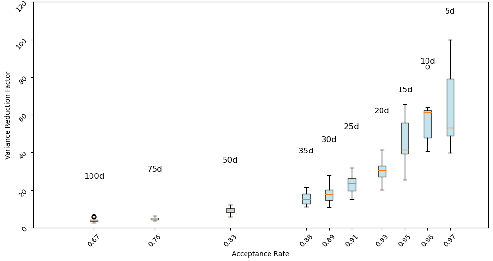
Figure 3: Boxplot of VRFs for the coordinate estimates of different dimensional Gaussian target and Gaussian proposal

In the Proof of Theorem 2 we have derived that the asymptotic variance $\sigma_{IMCV}^{2}$ can be bounded by $C^{\star}\mathbb{KL}(q(x)\|\pi(x))^{1/4}$. Thus, since $\sigma_{F}^{2}=1$,

$$VRF=\frac{\sigma_{F}^{2}}{\sigma_{IMCV}^{2}}\gtrsim{C^{\star}}^{-1}\left[\frac{1}{2}\left(\sigma_{\gamma}^{2}+\frac{1}{2}\sigma_{\delta}^{2}\right)d\right]^{-1/4}.$$

Therefore, with the increase of the dimensions, the decrease rate of the variance reduction factor is no faster than $O(d^{-1/4})$ asymptotically. Moreover, increased precision in adaptation correlates with the amplification in the VRF.

Appendix D Adaptive IM algorithm with KL divergence instance

In all three experiments of Section 3.3 we use the adaptation algorithm combined with doubly stochastic variational inference (DSVI) (Titsias and Lázaro-Gredilla, 2014) and Adam optimisation (Kingma and Ba, 2014). The specific algorithm is described here in Algorithm 3.

Algorithm 3 Adaptive IM with DSVI and Adam

Inputs: Gaussian proposal parameters $\theta=(\mu,\boldsymbol{L})$, log-pdf of target distribution $\log\pi(x)$, stepsizes for two parameters ($\alpha,\beta$), batch size $B$, the number of batches $\ell$, objective function $F$.
Initialisation Set $i\leftarrow 0,j\leftarrow 0$ and initialise {$X$, $\theta=(\mu,\boldsymbol{L})$, $\alpha$, $\beta$} by {$X_{0}$, $q_{\theta_{0}}=(\mu_{0},\boldsymbol{L}_{0})$, $\alpha_{0}$, $\beta_{0}$}.

1:while $i<\ell$ do

2:     Generate diagonal matrix: $\boldsymbol{\Delta}_{\boldsymbol{L}_{i}}\leftarrow\text{diag}(\text{diag}(\boldsymbol{L}_{i}))$.

3:     while $j<B$ do

4:         Sample $Z_{ij}$ from $\mathcal{N}(z|0,\boldsymbol{I}_{d})$.

5:         Compute $Y_{ij}\leftarrow\mu_{i}+L_{i}Z_{i}$.

6:         Save $\{\alpha(X_{ij},Y_{ij}),X_{ij},Y_{ij}\}$ from independent Metropolis $IM(P_{i},\pi,q_{\theta_{i}})$.

7:         Update function $H_{\mu}(Y_{ij})\leftarrow\nabla\log\pi(Y_{ij})$, $H_{L}(Y_{ij},Z_{ij})\leftarrow\nabla\log\pi(Y_{i})Z_{i}^{\top}+\boldsymbol{\Delta}_{\boldsymbol{L}_{i}}$.

8:         Set $j\leftarrow j+1$.

9:     end while

10:     Adaptation update

$$\begin{cases}\mu_{i+1}\leftarrow\mu_{i}-\alpha_{i}Adam(\sum_{j=1}^{B}H_{\mu}(Y_{ij})/B),\\ L_{i+1}\leftarrow L_{i}-\beta_{i}Adam(\sum_{j=1}^{B}H_{L}(Y_{ij},Z_{ij})/B).\end{cases}$$

11:     Calculate analytical result for the batch $E_{q_{\theta_{i}}}[F]$.

12:     Update $i\leftarrow i+1,j\leftarrow 0$.

13:end while

14:Calculate coefficients given by (28) and (29) for each batch.

15:Calculate the estimator (27).

Returns: An estimate for (27).

References

• Alexopoulos et al. (2023) Alexopoulos, A., Dellaportas, P. and Titsias, M. K. (2023) Variance reduction for metropolis–hastings samplers. Statistics and Computing, 33(1), 6.
• Andradóttir et al. (1993) Andradóttir, S., Heyman, D. P. and Ott, T. J. (1993) Variance reduction through smoothing and control variates for markov chain simulations. ACM Transactions on Modeling and Computer Simulation (TOMACS), 3(3), 167–189.
• Andrieu and Moulines (2006) Andrieu, C. and Moulines, É. (2006) On the ergodicity properties of some adaptive mcmc algorithms. Annals of Applied Probability, 16(3), 1462–1505.
• Andrieu and Roberts (2009) Andrieu, C. and Roberts, G. O. (2009) The pseudo-marginal approach for efficient monte carlo computations. The Annals of Statistics, 37(2), 697–725.
• Andrieu and Thoms (2008) Andrieu, C. and Thoms, J. (2008) A tutorial on adaptive mcmc. Statistics and Computing, 18(4), 343–373.
• Assaraf and Caffarel (1999) Assaraf, R. and Caffarel, M. (1999) Zero-variance principle for monte carlo algorithms. Physical Review Letters, 83(23), 4682–4685.
• Atchadé and Perron (2005) Atchadé, Y. F. and Perron, F. (2005) Improving on the independent metropolis-hastings algorithm. Statistica Sinica, 15(1), 3–18.
• Barp et al. (2022) Barp, A., Oates, C. J., Porcu, E. and Girolami, M. (2022) A Riemann–Stein kernel method. Bernoulli, 28(4), 2181 – 2208.
• Belomestny et al. (2020) Belomestny, D., Iosipoi, L., Moulines, E., Naumov, A. and Samsonov, S. (2020) Variance reduction for markov chains with application to mcmc. Statistics and Computing, 30(4), 973–997.
• Brofos et al. (2022) Brofos, J., Gabrié, M., Brubaker, M. A. and Lederman, R. R. (2022) Adaptation of the independent metropolis-hastings sampler with normalizing flow proposals. In International Conference on Artificial Intelligence and Statistics, 5949–5986. PMLR.
• Cappé et al. (2008) Cappé, O., Douc, R., Guillin, A., Marin, J.-M. and Robert, C. P. (2008) Adaptive importance sampling in general mixture classes. Statistics and Computing, 18, 447–459.
• Cornebise et al. (2008) Cornebise, J., Moulines, É. and Olsson, J. (2008) Adaptive methods for sequential importance sampling with application to state space models. Statistics and Computing, 18(4), 461–480.
• Dellaportas et al. (2012) Dellaportas, P., Forster, J. J. and Ntzoufras, I. (2012) Joint specification of model space and parameter space prior distributions. Statistical Science, 232–246.
• Dellaportas and Kontoyiannis (2009) Dellaportas, P. and Kontoyiannis, I. (2009) Notes on using control variates for estimation with reversible mcmc samplers. arXiv preprint arXiv:0907.4160.
• Dellaportas and Kontoyiannis (2012) — (2012) Control variates for estimation based on reversible Markov chain Monte Carlo samplers. Journal of the Royal Statistical Society: Series B (Statistical Methodology), 74(1), 133–161.
• Dellaportas and Tsionas (2019) Dellaportas, P. and Tsionas, M. G. (2019) Importance sampling from posterior distributions using copula-like approximations. Journal of Econometrics, 210(1), 45–57.
• Filippone and Girolami (2014) Filippone, M. and Girolami, M. A. (2014) Pseudo-marginal bayesian inference for gaussian processes. IEEE Transactions on Pattern Analysis and Machine Intelligence, 36, 2214–2226.
• Gabrié et al. (2022) Gabrié, M., Rotskoff, G. M. and Vanden-Eijnden, E. (2022) Adaptive Monte Carlo augmented with normalizing flows. Proceedings of the National Academy of Sciences of the United States of America, 119(10), e2109420119.
• Geffner and Domke (2020) Geffner, T. and Domke, J. (2020) Approximation based variance reduction for reparameterization gradients. In Advances in Neural Information Processing Systems (eds. H. Larochelle, M. Ranzato, R. Hadsell, M. Balcan and H. Lin), vol. 33, 2397–2407. Curran Associates, Inc. URL: https://proceedings.neurips.cc/paper_files/paper/2020/file/193002e668758ea9762904da1a22337c-Paper.pdf.
• Geyer (1992) Geyer, C. J. (1992) Practical markov chain monte carlo. Statistical Science, 7(4), 473–483.
• Gianniotis et al. (2016) Gianniotis, N., Schnörr, C., Molkenthin, C. and Bora, S. (2016) Approximate variational inference based on a finite sample of gaussian latent variables. Pattern Analysis and Applications, 19, 475–485.
• Girolami and Calderhead (2011) Girolami, M. and Calderhead, B. (2011) Riemann manifold Langevin and Hamiltonian Monte Carlo methods. Journal of the Royal Statistical Society. Series B: Statistical Methodology, 73(2), 123–214.
• Haario et al. (2001) Haario, H., Saksman, E. and Tamminen, J. (2001) An adaptive Metropolis algorithm. Bernoulli, 7(2), 223–242.
• Harrison and Rubinfeld (1978) Harrison, D. and Rubinfeld, D. (1978) Hedonic Housing Prices and the Demand for Clean Air. Journal of Environmental Economics and Management, 5, 81–102.
• Henderson (1997) Henderson, S. G. (1997) Variance reduction via an approximating Markov process. Stanford University.
• Holden et al. (2009) Holden, L., Hauge, R. and Holden, M. (2009) Adaptive independent Metropolis-Hastings. Annals of Applied Probability, 19(1), 395–413.
• Jacob et al. (2011) Jacob, P., Robert, C. P. and Smith, M. H. (2011) Using parallel computation to improve independent metropolis–hastings based estimation. Journal of Computational and Graphical Statistics, 20(3), 616–635.
• Kahn and Marshall (1953) Kahn, H. and Marshall, A. W. (1953) Methods of reducing sample size in monte carlo computations. Journal of the Operations Research Society of America, 1(5), 263–278.
• Kass and Raftery (1995) Kass, R. E. and Raftery, A. E. (1995) Bayes factors. Journal of the American Statistical Association, 90(430), 773–795.
• Kingma and Ba (2014) Kingma, D. P. and Ba, J. (2014) Adam: A method for stochastic optimization. arXiv preprint arXiv:1412.6980.
• Kingma and Welling (2013) Kingma, D. P. and Welling, M. (2013) Auto-encoding variational bayes. arXiv preprint arXiv:1312.6114.
• Kipnis and Varadhan (1986) Kipnis, C. and Varadhan, S. R. (1986) Central limit theorem for additive functionals of reversible Markov processes and applications to simple exclusions. Communications in Mathematical Physics, 104(1), 1–19.
• Kucukelbir et al. (2017) Kucukelbir, A., Tran, D., Ranganath, R., Gelman, A. and Blei, D. M. (2017) Automatic differentiation variational inference. J. Mach. Learn. Res., 18(1), 430–474.
• Lázaro-Gredilla et al. (2010) Lázaro-Gredilla, M., Quiñnero-Candela, J., Rasmussen, C. E. and Figueiras-Vidal, A. R. (2010) Sparse spectrum gaussian process regression. Journal of Machine Learning Research, 11(63), 1865–1881.
• Liang et al. (2008) Liang, F., Paulo, R., Molina, G., Clyde, M. A. and Berger, J. O. (2008) Mixtures of g priors for bayesian variable selection. Journal of the American Statistical Association, 103(481), 410–423.
• Liang et al. (2022) Liang, X., Livingstone, S. and Griffin, J. (2022) Adaptive random neighbourhood informed markov chain monte carlo for high-dimensional bayesian variable selection. Statistics and Computing, 32(5), 84.
• Liu (1996) Liu, J. S. (1996) Metropolized independent sampling with comparisons to rejection sampling and importance sampling. Statistics and Computing, 6(2), 113–119.
• McCulloch and Rossi (1992) McCulloch, R. E. and Rossi, P. E. (1992) Bayes factors for nonlinear hypotheses and likelihood distributions. Biometrika, 79(4), 663–676.
• Meyn (2008) Meyn, S. (2008) Control techniques for complex networks. Cambridge University Press.
• Miller et al. (2017) Miller, A., Foti, N., D' Amour, A. and Adams, R. P. (2017) Reducing reparameterization gradient variance. In Advances in Neural Information Processing Systems (eds. I. Guyon, U. V. Luxburg, S. Bengio, H. Wallach, R. Fergus, S. Vishwanathan and R. Garnett), vol. 30. Curran Associates, Inc. URL: https://proceedings.neurips.cc/paper_files/paper/2017/file/325995af77a0e8b06d1204a171010b3a-Paper.pdf.
• Mira et al. (2013) Mira, A., Solgi, R. and Imparato, D. (2013) Zero variance Markov chain Monte carlo for Bayesian estimators. Statistics and Computing, 23(5), 653–662.
• Murray and Adams (2010) Murray, I. and Adams, R. P. (2010) Slice sampling covariance hyperparameters of latent gaussian models. Advances in neural information processing systems, 23.
• Naesseth et al. (2020) Naesseth, C., Lindsten, F. and Blei, D. (2020) Markovian score climbing: Variational inference with ${KL}(p\parallel q)$. Advances in Neural Information Processing Systems, 33, 15499–15510.
• Newton and Raftery (1994) Newton, M. A. and Raftery, A. E. (1994) Approximate bayesian inference with the weighted likelihood bootstrap. Journal of the Royal Statistical Society Series B: Statistical Methodology, 56(1), 3–26.
• Oates et al. (2019) Oates, C. J., Cockayne, J., Briol, F. X. and Girolami, M. (2019) Convergence rates for a class of estimators based on Stein’s method. Bernoulli, 25(2), 1141–1159.
• Oates et al. (2017) Oates, C. J., Girolami, M. and Chopin, N. (2017) Control functionals for Monte Carlo integration. Journal of the Royal Statistical Society. Series B: Statistical Methodology, 79(3), 695–718.
• Owen (2013) Owen, A. B. (2013) Monte Carlo theory, methods and examples. Stanford.
• Paananen et al. (2021) Paananen, T., Piironen, J., Bürkner, P. C. and Vehtari, A. (2021) Implicitly adaptive importance sampling. Statistics and Computing, 31(2), 16.
• Papamarkou et al. (2014) Papamarkou, T., Mira, A., Girolami, M. et al. (2014) Zero variance differential geometric Markov chain Monte Carlo algorithms. Bayesian Analysis, 9(1), 97–128.
• Ranganath et al. (2014) Ranganath, R., Gerrish, S. and Blei, D. (2014) Black box variational inference. In International Conference on Artificial Intelligence and Statistics, 814–822.
• Rezende et al. (2014) Rezende, D. J., Mohamed, S. and Wierstra, D. (2014) Stochastic backpropagation and approximate inference in deep generative models. In Proceedings of the 31st International Conference on Machine Learning. PMLR.
• Richard and Zhang (2007) Richard, J. F. and Zhang, W. (2007) Efficient high-dimensional importance sampling. Journal of Econometrics, 141(2), 1385–1411.
• Robbins and Monro (1951) Robbins, H. and Monro, S. (1951) A Stochastic Approximation Method. The Annals of Mathematical Statistics, 22(3), 400–407.
• Robert et al. (2018) Robert, C. P., Elvira, V., Tawn, N. and Wu, C. (2018) Accelerating mcmc algorithms. Wiley Interdisciplinary Reviews: Computational Statistics, 10(5), e1435.
• Roberts and Rosenthal (2007) Roberts, G. O. and Rosenthal, J. S. (2007) Coupling and ergodicity of adaptive Markov chain Monte Carlo algorithms. Journal of Applied Probability, 44(2), 458–475.
• Roberts and Rosenthal (2009) — (2009) Examples of adaptive MCMC. Journal of Computational and Graphical Statistics, 18(2), 349–367.
• Roeder et al. (2017) Roeder, G., Wu, Y. and Duvenaud, D. K. (2017) Sticking the landing: Simple, lower-variance gradient estimators for variational inference. In Advances in Neural Information Processing Systems (eds. I. Guyon, U. V. Luxburg, S. Bengio, H. Wallach, R. Fergus, S. Vishwanathan and R. Garnett), vol. 30. Curran Associates, Inc. URL: https://proceedings.neurips.cc/paper_files/paper/2017/file/e91068fff3d7fa1594dfdf3b4308433a-Paper.pdf.
• Rosenthal (2003) Rosenthal, J. S. (2003) Asymptotic variance and convergence rates of nearly-periodic markov chain monte carlo algorithms. Journal of the American Statistical Association, 98(461), 169–177.
• Salimans and Knowles (2013) Salimans, T. and Knowles, D. A. (2013) Fixed-form variational posterior approximation through stochastic linear regression. Bayesian Analysis, 8(4), 837–882.
• Smith and Tierney (1996) Smith, R. and Tierney, L. (1996) Exact transition probabilities for the independence Metropolis sampler. Preprint.
• South et al. (2022) South, L. F., Karvonen, T., Nemeth, C., Girolami, M. and Oates, C. J. (2022) Semi-exact control functionals from Sard’s method. Biometrika, 109(2), 351–367.
• South et al. (2023) South, L. F., Oates, C. J., Mira, A. and Drovandi, C. (2023) Regularized zero-variance control variates. Bayesian Analysis, 18(3), 865–888.
• Tan and Nott (2018) Tan, L. S. L. and Nott, D. J. (2018) Gaussian variational approximation with sparse precision matrices. Statistics and Computing, 28(2), 259–275.
• Tan (2006) Tan, Z. (2006) Monte carlo integration with acceptance-rejection. Journal of Computational and Graphical Statistics, 15(3), 735–752.
• Titsias and Dellaportas (2019) Titsias, M. K. and Dellaportas, P. (2019) Gradient-based adaptive markov chain monte carlo. In Advances in Neural Information Processing Systems, vol. 32.
• Titsias and Lázaro-Gredilla (2014) Titsias, M. K. and Lázaro-Gredilla, M. (2014) Doubly stochastic variational bayes for non-conjugate inference. In Proceedings of the 31st International Conference on Machine Learning. PMLR.
• Valle and Leisen (2010) Valle, L. D. and Leisen, F. (2010) A new multinomial model and a zero variance estimation. Communications in Statistics—Simulation and Computation®, 39(4), 846–859.
• Wang (2022) Wang, G. (2022) Exact convergence analysis of the independent Metropolis-Hastings algorithms. Bernoulli, 28(3), 2012–2033.