Magnetic Force Microscopy: High Quality Factor Two-Pass Mode

Abstract

Magnetic force microscopy (MFM) is a well-established technique in scanning probe microscopy (SPM) that allows the imaging of magnetic samples with spatial resolution of tens of nm and stray fields down to the mT range. Spatial resolution and field sensitivity can be improved significantly by measuring in vacuum conditions. This effect originates from the higher quality factor (Q-factor) of the cantilevers oscillation in vacuum compared to ambient conditions. However, while high Q-factors are desirable as they directly improve the magnetic measurement signal, they pose a challenge when pursuing a standard MFM two-pass (lift) mode measurement. At high Q-factors amplitude-based topography measurements become impossible and MFM phase response behaves non-linear. Here we present an implementation of a modified two-pass mode into a vacuum atomic force microscope (AFM) that overcomes these issues. By controlling Q in the first pass and using a phase-locked loop (PLL) technique in the second pass, high Q-factor measurements in vacuum are enabled. By measuring the cantilevers frequency shift instead of phase shift, otherwise emerging non-linearities are eliminated. The achievable improvements in resolution and sensitivity are demonstrated on patterned magnetic nanostructured samples. Elimination of non-linear response is showcased by a measurement of a very well-known calculable multilayer reference sample that is used for tip calibration in quantitative MFM (qMFM).

I Introduction

Magnetic force microscopy (MFM) is a widely accessible, user-friendly, and common tool for the characterization of materials exhibiting magnetic micro- and nanostructures. It detects the interaction of a microscopic magnetically coated tip on an oscillating cantilever with the sample to map the emanating stray fields. By using well-known reference samples, quantitative measurements are possible.Hu et al. ; Hug et al. ; van Schendel et al. ; Zhao et al. (a); Schwenk, Johannes ; Sakar et al. (2021); Feng et al. (a) Recently, an IEC standard on quantitative MFM measurements under ambient conditions was published.IEC (2021)

Initially, MFM development was boosted by the need of the industry to analyze and characterize magnetic data storage media. Babcock et al. However, novel magnetic materials that are in the focus of research are becoming increasingly challenging to characterize: Magnetic data storage is evolving, not only by pushing the density of magnetic data to the physical limits Morris (2021), but in particular by focusing on new ways of storing data. Concepts for storing data and computing based on nanoscale magnetic objects like domain walls or skyrmions, which are nm-scale topological stable magnetic vortexes, are topic of current research.Luo and You Furthermore, fundamental magnetic material research on multilayers for spintronic applications, vortices or 2D materials is increasingly dealing with very low stray fields and nanoscale structures.Liu et al. (2023) Consequently, also MFM itself needs to evolve.

The spatial resolution and field sensitivity of MFM can be significantly enhanced by measuring under vacuum conditions.Feng et al. (b) This results from the higher cantilever quality factors in vacuum in dynamic mode, directly leading to an increase in the measurements signal to noise ratio (SNR). However, advanced feedback techniques are required for stable operation in vacuum. MFM measurements are typically performed in a two-pass lift mode, where the tip-sample interaction is monitored in the second, lifted pass via the detection of the phase shift of the cantilever oscillation. In vacuum, due to the high Q-factors, only a small amount of energy per oscillation cycle is dissipated. This makes the oscillation very sensitive to external forces, but at the same time hard to control, as the external forces can overpower the driving force of the oscillation and thus crash the tip.Albrecht et al. ; Meyer et al. While a high sensitivity is desired in the second pass for acquiring the magnetic image, in the first pass, where the tip is brought close to the surface to map the topography, the issue of tip crashing and thus tip damage must be addressed.

A way to circumvent these problems is to use bimodal magnetic force microscopy with capacitive tip-sample distance control as described by [Schwenk et al., ; Zhao et al., b], that uses an “frequency-modulated capacitive tip-sample distance control mode”.Feng et al. (b) This technique ensures that the tip is always lifted and is, in particular, not requiring a first pass that is prone to tip crashing (hence it will be referred to in this work as single-pass mode). Even though this technique is an elegant operation-mode, it is not easy to implement and only suitable for electrical conducting samples that are flat on the nm scale.

Figure 1: Schematic overview of the new two-pass dual-mode setup. In normal operation the AFMs integrated internal lock-in amplifier Lock-In 1 is used, providing amplitude and phase-shift signal. To enable phase-locked loop measurements a second Lock-In 2 with PLL option is used. In lift mode (second pass) the drive signal applied to the modulation piezo (Piezo MOD) can be switched from the internal lock-in’s oscillator to the external Lock-In 2. The switching is achieved by a micro-controller operated switching box, that connects the source of the excitation signal accordingly to the line and lift mode state signal of the microscope.

We here present an implementation of a modified two-pass lift mode into a Park Systems NX-Hivac Atomic Force Microscope that enables measurements in vacuum conditions with high magnetic sensitivity and stable topography detection. While in the first pass the so-called Q-Control is utilized to artificially lower the Q-factor to a degree that the feedback loop can handle, in the second pass (lift mode) the measurements are done using an external lock-in amplifier running a phase-locked loop (PLL) to track the frequency shift of the cantilever oscillation. A simple overview over this new setup is outlined in Fig. 1. This technique allows to use the largest achievable Q-factor in the second pass and thus to utilize the maximum possible sensitivity for magnetic stray field measurements.

II Theory

The two-pass mode (also called lift mode or interleave mode by some manufacturers) is very well known and regarded as the workhorse of MFM.Meyer et al. It’s basics are explained in a variety of textbooks and articles concerned with the topic.Meyer et al. ; Voigtländer ; Haugstad ; Kazakova et al. (2019); Winkler et al. (2023) We assume therefore that two-pass mode is known to the reader and start the discussion by introducing the Q-factor. From there, the less commonly known Q-ControlRodrıguez and Garcıaa (2003); Hölscher and Schwarz operation is introduced, that shows some downsides for MFM phase-shift measurements in vacuum.

II.1 Q-factor

The Q-factor, that describes the degree of damping of an oscillating system, plays a central role for the MFM measurement sensitivity. The Q-factor can be described in terms of the stored energy definition as the ratio of the energy stored in the oscillation to energy dissipated per oscillation cycle.Voigtländer

In the case of atomic force microscopy, vacuum conditions lead to higher Q-factors since the density of gaseous particles decreases, reducing collisions with the oscillating cantilever (effectively reducing friction). Thus, less energy is dissipated, and the Q-factor rises. For high Q-factors, Q can equivalently be described by the bandwidth definition:

$$Q=\frac{f_{0}}{\Delta f_{\textrm{FWHM}}}$$ (1)

with resonance frequency $f_{0}$ and resonance full width at half maximum (FWHM) $\Delta f_{\textrm{FWHM}}$. Using the latter definition, the Q-factor can be easily derived from the non-contact frequency sweep data, an example is shown as in Fig. 2. With rising Q-factors, the width of the resonance peak is reduced, yielding the response of the resonantly oscillating cantilever more susceptible to external forces which increases sensitivity. Commercial MFM cantilevers usually reach Q-factors of 200 in ambient conditions, whereas in vacuum Q-factors up to 20 000 are possible. Using specially manufactured vacuum cantilevers even higher Q-factors up to 200 000 are achievable.Meyer et al.

In the case of high Q-factors (> 2000), the oscillation is only weakly damped, and the amplitude becomes increasingly hard to stabilize against parameter changes, as can be seen in the frequency sweep in Fig. 2. As only very little energy is dissipated per cycle, transient processes emerge. Consequently, the cantilever will keep its frequency, despite the driving frequency already moving on (this effect is known as ringing, or also as transient, requiring some settling time for the system to return into the steady state of harmonic oscillation).

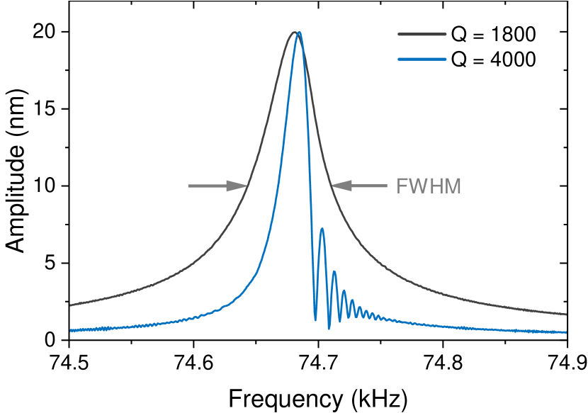
Figure 2: Ringing due to high Q-factor. Experimentally acquired frequency sweep data. Both curves were obtained with Q-control enabled, once with high Q-control attenuation (black curve, $Q\approx 1800$) and low attenuation (blue curve, $Q\approx 4000$). After reaching resonance at $f_{0}=74.68$ kHz ringing can be observed in the blue curve, inhibiting operation in amplitude-based non-contact mode.

Q-factors can be artificially damped in vacuum conditions to avoid this issue by means of the so-called Q-control mechanism discussed in Chap. II.3.

II.2 Signal generation in MFM

In dynamic mode, the cantilever is exited at its resonance frequency (or close to it). In the most simplistic way the motion $z(t)$ of the free cantilever (that is not sensing a force) can be expressed by the well-known equation of the driven harmonic oscillator

$$m\ddot{z}(t)+m\gamma\dot{z}(t)+c_{\textrm{z}}(z(t)-d)=F_{0}\cos(2\pi f_{\textrm{d}}t)$$ (2)

with the mass m, damping coefficient $\gamma$, spring constant $c_{\textrm{z}}$, the tips equilibrium position $d$, and driving force $F_{0}=a_{\textrm{d}}c_{\textrm{z}}$ operating at driving amplitude $a_{\textrm{d}}$ and driving frequency $f_{\textrm{d}}$. The resonance frequency of the undisturbed oscillator is given by $f_{0}=\frac{1}{2\pi}\sqrt{c_{\textrm{z}}/m}$. The damping factor $\gamma$ can be described using the quality factor $Q_{0}$ of the undisturbed oscillator that is only interacting with its environmental gas as $\gamma=2\pi f_{0}/Q_{0}$ for frequencies close to the resonance frequency $f\approx f_{0}$. With the ansatz $z(t)=A\cos(2\pi ft+\varphi)$ the amplitude $A$ and phase $\varphi$ for the differential equation can be found as

$$A(f) =\frac{F_{0}/(4\pi m)}{\sqrt{(f_{0}^{2}-f^{2})^{2}+(f_{0}f/Q_{0})^{2}}}$$ (3)

$$\varphi(f) =\arctan\left(-\frac{f_{0}f}{Q_{0}(f_{0}^{2}-f^{2})}\right)$$ (4)

Basic observations are that the amplitude reaches its maximum for $f=f_{0}$ and is only restricted by the damping $\gamma$. Importantly, the phase does not depend on the driving force, as it only affects the amplitude. A typical (experimentally obtained) curve of $A$ and $\varphi$ can be in seen Fig. 6, as discussed later.

II.3 Q-control

To utilize the oscillating tip for non-contact mode AFM measurements external forces interacting with tip must be taken into account. Moreover, an additional term is required if the Q-factor is to be artificially reduced, i.e. to achieve Q-control. A more complete version of Eq. 2 in regards of AFM is then given in [Hölscher and Schwarz, ]:

$$m\ddot{z}(t)+\frac{2\pi f_{0}m}{Q_{0}}\dot{z}(t)+c_{\textrm{z}}(z(t)-d)+\underbrace{gc_{\textrm{z}}z(t-t_{0})}_{\textrm{Q-Control}}$$

$$=\underbrace{a_{\textrm{d}}c_{\textrm{z}}\cos(2\pi f_{\textrm{d}}t)}_{\textrm{external driving force}}+\underbrace{F_{\textrm{ts}}[z(t),\dot{z}(t)]}_{\textrm{tip-sample force}}$$ (5)

The first of the two new terms is the Q-Control term with the gain factor g and signal shift $t-t_{0}$. The tip-sample force $F_{\textrm{ts}}$ depends not only on the tip position $z(t)$ but also its derivative $\dot{z}(t)$. Solving this equation requires further assumptions as discussed in [Hölscher and Schwarz, ]. One import result is that, in fact, the Q-factor can be can be controlled by adjusting the gain factor, resulting in an effective $Q_{\textrm{eff}}$ that is given by (assuming for simplicity $F_{\textrm{ts}}=0$ and $f_{\textrm{d}}\approx f_{0}$):

$$Q_{\textrm{eff}}(g,t_{0})=\frac{1}{1/Q_{0}-g\sin(2\pi f_{\textrm{d}}t_{0})}.$$ (6)

The experimental setup realization is schemed in Fig. 3. By adding a feedback loop (colored blue) to the modulation piezo, so-called Q-control operation is possible. By amplifying and phase-shifting (e.g. time-shifting) the detected signal, energy loss can be compensated or induced, thus amplifying or attenuating Q.

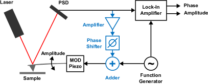
Figure 3: Q-control in AFM. The cantilever is excited via a function generator driving the modulation piezo. Induced oscillation is measured using the reflected laser-pointer signal on a position sensitive photodiode. The electric signal is feed to a lock-in amplifier, measuring phase (relative to the function generator) and amplitude. By inserting an additional feedback path via an amplifier and phase shifter (colored blue) the driving signal can be modified and Q can be controlled.

II.4 Tip-sample force, frequency, and phase shift

The second term in Eq. II.3 describes the influence of external forces. In case of the force free driven oscillator the resonance frequency $f_{0}$ was introduced as

$$f_{0}=\frac{1}{2\pi}\sqrt{\frac{k}{m}}.$$ (7)

However, an external force acting on the tip will shift the cantilever resonance frequency. In typical cases, where (i) the tips oscillation amplitude is small compared to the scale of the spatial variation of the tip-sample force $F_{\textrm{ts}}$ and where (ii) the cantilevers restoring force behaves like a Hookean spring $F_{\textrm{cantilever}}=-k_{0}(s_{\textrm{z}}-s_{\textrm{z}_{0}})$ (with the tip displacement $s_{\textrm{z}}-s_{\textrm{z}_{0}}$ around the equilibrium position $s_{\textrm{z}_{0}}$) and (iii) the restoring force is largeHaugstad , the impact of the force acting on the tip can be described as modification of the spring constant

$$k=k_{0}+k^{\prime}=k_{0}-\frac{\partial F_{\textrm{ts}}}{\partial s_{\textrm{z}}}$$ (8)

with the differential expressing the tip-sample force that acts on the tip while traveling the distance $s_{\textrm{z}}$ in Z-direction of the oscillation. Within this model, the resonance frequency depends on the tip-sample force:

$$f_{0}^{\prime}=\frac{1}{2\pi}\sqrt{\frac{k_{0}-\frac{\partial F_{\textrm{ts}}}{\partial s_{\textrm{z}}}\frac{k_{0}}{k_{0}}}{m}}=f_{0}\sqrt{1-\frac{1}{k_{0}}\frac{\partial F_{\textrm{ts}}}{\partial s_{\textrm{z}}}}$$ (9)

To the second part of the equation a Taylor-expansion $\sqrt{1-x}\approx 1-\frac{1}{2}x$ can be applied. As the deviation of $F_{\textrm{ts}}$ is very small compared to the initial spring constant $k_{0}$ this approximation is justified and $f_{0}^{\prime}$ thus can be approximated as

$$f_{0}^{\prime}\approx f_{0}\left(1-\frac{1}{2k_{0}}\frac{\partial F_{\textrm{ts}}}{\partial s_{\textrm{z}}}\right).$$ (10)

Therefore the frequency shift is directly proportional to the change of the tip-sample force:

$$\Delta f=f_{0}^{\prime}-f_{0}=\frac{f_{0}}{2k_{0}}\frac{\partial F_{\textrm{ts}}}{\partial s_{\textrm{z}}}.$$ (11)

In consequence, at constant excitation frequency $f$ the observed $\varphi$ (see Eq. 4), will experience a phase shift, as $f_{0}$ is not constant, but subject to change. This is the basic working principle of MFM in two-pass mode, as this phase shift is the measurement signal. Evaluating the first derivative of Eq. 4

$$\frac{\partial}{\partial f}\varphi(f)=\frac{-f_{0}Q_{0}(f^{2}+f_{0}^{2})}{Q_{0}^{2}(f^{2}-f_{0}^{2})^{2}+f^{2}f_{0}^{2}}$$ (12)

it can be argued that for small $Q_{0}$, large $f$ and limited variation of $f_{0}$ while $f\approx f_{0}$ it is reasonable to ignore the first term in the denominator, simplifying the equation to

$$\frac{\partial}{\partial f}\varphi(f\approx f_{0})=\frac{2Q_{0}}{f}$$ (13)

thus, showing a constant slope and in consequence linear signal response. This approximation often is sufficient for MFM operation in air, in common setups typically operating at $Q_{0}\approx 200$ and $f_{0}\approx 70$ kHz. Unfortunately, for large $Q_{0}$ this argumentation doesn’t hold up anymore and non-linear behaviour comes into play for vacuum operation.

II.5 Tip-sample force in MFM

In MFM the force acting on the magnetically coated tip with the local magnetization $\textbf{M}_{\textrm{tip}}(\textbf{r}^{\prime},z^{\prime})$ in the sample stray field $\textbf{H}_{\textrm{sample}}(\textbf{r}^{\prime},z^{\prime})$ can be described as a two-dimensional cross-correlation integral over the magnetic tip volumeHug et al.

$$\textbf{F}_{\textrm{mag}}(\textbf{r},z)= \mu_{0}\iint_{V^{\prime}}\left(\vec{\nabla}\cdot\textbf{M}_{\textrm{tip}}(\textbf{r}^{\prime},z^{\prime})\right)$$ (14)

$$\cdot\textbf{H}_{\textrm{sample}}(\textbf{r}+\textbf{r}^{\prime},z+z^{\prime})d\textbf{r}^{\prime}dz^{\prime}$$

with the in-plane coordinate vector $\textbf{r}=(x,y)$, measurement height $z$ and vacuum permeability $\mu_{0}$. By inserting this into Eq. 11, the relation between local magnetic field and frequency shift of the oscillating cantilever can be derived. Calculations are conveniently performed in a partial Fourier space with $(x,y,z)\rightarrow(k_{x},k_{y},z)$. This is, for example, discussed in detail in [Hu et al., ; Hug et al., ; van Schendel et al., ; Zhao et al., a; Schwenk, Johannes, ] and results in

$$\Delta f(\textbf{k},z)=-\frac{\mu_{0}f_{0}}{2c_{\textrm{z}}}\cdot\textrm{LCF}(\textbf{k},\theta,\phi,A_{0})$$

$$\cdot\frac{\partial\textbf{H}_{\textrm{z,tip}}^{*}(\textbf{k},z)}{\partial_{\textrm{z}}}\cdot\textbf{H}_{\textrm{z}_{\textrm{sample}}}(\textbf{k},z).$$ (15)

For $f\approx f_{0}$ and thus small $\Delta\varphi$ this gives

$$\Delta\varphi(\textbf{k},z)=-\frac{\mu_{0}Q}{c_{\textrm{z}}}\cdot\textrm{LCF}(\textbf{k},\theta,\phi,A_{0})$$

$$\cdot\frac{\partial\textbf{H}_{z,\textrm{tip}}^{*}(\textbf{k},z)}{\partial_{\textrm{z}}}\cdot\textbf{H}_{\textrm{z}_{\textrm{sample}}}(\textbf{k},z).$$ (16)

The here introduced lever correction function LCF accounts for cantilever- and device-specific parameters. It corrects for the canting angles $\theta$ and $\phi$ (see Fig. 4) and the finite oscillation amplitude $A_{0}$. The derivative of the complex conjugate of $H_{z,\textrm{tip}}$ describes the effective stray field gradient of the tip that is located in a plane parallel to the samples surface at measurement height $z$.

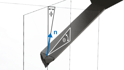
Figure 4: Canting angles due to cantilever tilt in MFM. Cantilevers are mounted at an angle $\theta$ to the sample surface, so that only the tip at the end of the cantilever will interact with the sample. Thus, the normal vector n of the cantilever and therefore the tip is not aligned with the normal vector of the sample, which needs to be taken into account for quantitative evaluation. Furthermore the cantilever might be installed twisted or/and the sample not mounted evenly, accounted for by the angle $\phi$.

Consequently, damping the Q-factor in MFM phase shift measurements results in a proportional reduction of the phase signal while inducing additional noise-generating electronics, thus lowering the SNR even further. While the phase shift signal improvement is directly linked to the quality factor ($\varphi\propto Q$) in case of frequency shift this is obviously not the case as Eq. 15 is independent from $Q$. To understand the SNR improvement for frequency shift, a closer look at the origin of noise in AFM is required.

Thermal noise due to thermal induced cantilever motion in AFM allows the detection of signals with the minimum detectable force gradient

$$\frac{\partial F_{\textrm{min}}^{\prime}}{\partial z}=\sqrt{\frac{4k_{\textrm{L}}k_{\textrm{B}}TB}{2\pi f_{0}Q\langle A_{\textrm{osc}}^{2}\rangle}}$$ (17)

with the cantilever force constant $k_{\textrm{L}}$, the Boltzmann constant $k_{\textrm{B}}$, the absolute temperature $T$, the bandwidth $B$ and the mean-square of the oscillation amplitude $\langle A_{\textrm{osc}}^{2}\rangle$. Depending on whether static or dynamic mode with amplitude or frequency modulation is used a factor of $\sqrt{2}$ applies, further reading in [Albrecht et al., ; Voigtländer, ].

From this equation it is clear, that a large Q-factor is desirable to improve sensitivity. However, a large Q-factor also impacts the required bandwidth in amplitude modulated (AM) operation: If an external force acts on the cantilever (thus changing the resonance frequency $f_{0}$), the oscillating systems needs time to reach the new steady state. The required time for the system response can be expressed by the time constant $\tau\approx 2Q/\omega_{0}=Q/(\pi f_{0})$. Consequently, for phase shift measurements bandwidth and quality factor are not independent, therefore measurement with high Q-factors become unacceptably slow. This does not hold true for frequency shift measurements, as by tracing $f_{0}$, the issue of settling time can be avoided. The bandwidth will only be limited by the demodulation system used for frequency modulation (FM) and not by the transient behavior.

On a side note, it shall be mentioned, that also increasing the oscillation amplitude would improve the minimum detectable force gradient (Eq. 17), but as for quantitative evaluation the external force must remain (reasonably) constant within the cantilever oscillation, the actual usable amplitude range is limited below its experimental limits.

III Experimental

In the following section the new modified two-pass mode operation is introduced, which will be referred to as two-pass dual-mode, as it allows phase shift measurements with a dampened Q, as well as frequency shift measurements at high Q in situ. By measuring frequency shift (instead of phase shift) in the second pass, the highest possible Q can be used without suffering sensitivity loss or experiencing non-linearity in measurement signals. This is demonstrated on a structured sample and a thin film multilayer system forming domain walls.

III.1 Phase and Frequency detection

III.1.1 First pass: Topography

Fig. 5 shows the working principle of amplitude-controlled topography measurements, as used in the first pass of two-pass mode. The free oscillating cantilever shows a resonance peak as indicated by the solid plotted curve with resonance frequency $f_{0}$. For operation in non-contact mode the drive frequency $f_{\textrm{d}}$ must be greater than $f_{0}$. The drive frequency has been chosen such, that the desired amplitude setpoint $A_{\textrm{s}}$ is achieved. By bringing the oscillating tip close to the surface, external forces will change the resonance frequency, for example from $f_{0}$ to $f_{0}^{\prime}$, changing the resonance behaviour by $\Delta f$. This causes a amplitude change $\Delta A$ at the fixed drive frequency $f_{\textrm{d}}$, which is used as feedback for the Z-piezo. The controller will retract or extend the Z-piezo so that the setpoint amplitude $A_{\textrm{s}}$ is reached again. The required piezo movement maps the topography of the sample. This works well for low Q-factors (for example $Q\approx 200$) , as the resonance peak has a FWHM of around 350 Hz while the frequency shift amounts to some 10 Hz.

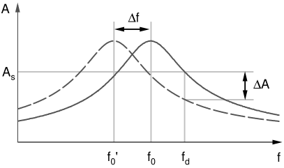
Figure 5: Topography acquisition via amplitude modulation. The free oscillating cantilever will show a resonance curve around $f_{0}$ (solid line). Under the impact of external forces, the resonance frequency will shift (for example) from $f_{0}$ to $f_{0}^{\prime}$, shifting the whole resonance curve by $\Delta f$ (dashed line). This shift of the resonant behaviour will lead to a amplitude change $\Delta A$ at fixed drive frequency $f_{\textrm{d}}$. By feeding this amplitude change into a feedback loop, ensuring by movement of the Z-piezo that the amplitude stays at setpoint $A_{\textrm{s}}$, the samples topography can be measured.

III.1.2 Second pass: Magnetic signal

In the second pass (in lift mode) the AFM controller retraces the topography that was acquired in the first pass (adding a user defined lift height). The magnetic interaction leads to a frequency shift of the cantilever’s resonance frequency. In MFM the magnetic interaction between tip and sample is detected by either keeping the excitation frequency constant and monitoring the phase shift or by tracking the change of the resonance frequency. In Fig. 6 these two cases are portrayed using experimentally obtained frequency sweep data for operation in air. The black curve shows the amplitude, blue the corresponding phase. The phase shift at the resonance was adjusted in post-processing to match -90 deg.

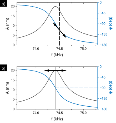
Figure 6: MFM operation with (a) phase and (b) frequency shift detection. In (a) phase shift detection is schemed as used in common MFM two-pass operation. Operation is slightly off the resonance frequency (for tapping mode left of the peak, in non-contact mode, as here the case, right of the peak). In lift mode at this setpoint (vertical dotted line) the phase shift is measured. Near the resonance peak the phase response behaves nearly linear (indicated by the arrow). Case (b) shows the detection of frequency shift. The corresponding phase value to the peak is used as setpoint. This enables tracking of the peak and thus the resonance frequency. As the phase always stays the same (ensured by the PLL), the problems of non-linearity are eliminated.

In ambient conditions, detection via phase shift is common, as pictured in 6 (a). As for low Q-factors, the measured phase shift is rather small and usually in the range of single digit degrees, the phase response is staying in the range of approximately linear behaviour (indicated by the arrow).

In vacuum conditions, by contrast, measurement signals of tens of degrees are possible, clearly leaving the area of linearity, rendering the data useless for quantitative measurements. Therefore, in vacuum operation frequency shift measurements are used, eliminating this issue. The resonance frequency (indicated by the vertical line in Fig. 6 (b) that can move in either way) is measured by picking the corresponding phase at resonance as setpoint (here at -90 deg, indicated by the horizontal line). A phase-locked loop (PLL) is utilized to adjust the frequency of the excitation, so that the actual phase is kept at the desired phase-setpoint, thus tracking the resonance frequency peak.

III.2 Modified Two-Pass Mode “Two-Pass Dual-Mode”

The idea behind the new two-pass dual-mode is to vary the Q-factor and signal detection scheme in between the two-passes. This allows to optimize the measurement for stability while acquiring topography and yet boost sensitivity when measuring magnetic stray fields in lift mode. The measurement system used in this work consists of a Park Systems NX-Hivac AFM equipped with a signal extension module (SAM) that allows to tap and modify signals. The topography is always measured with Park’s built-in Q-control, while in the second pass a Zurich Instruments HF2LI lock-in amplifier with dual PLL is option used, allowing to tailor settings suitable for high Q-factor frequency shift detection in vacuum operation.

In lift mode, the AFM controls the lift height via the Z-piezo but does not modulate the drive piezo signal, thus the drive piezo can be switched to the external HF2LI while in lift mode. Signal lock at the HF2LI is achieved in a couple of 100 µs, meaning that switching can take place during overscan (scanning a user-defined percentage over the desired scan area to avoid turnaround streaks at the edges of the final image). The HF2LI excites and tracks the frequency of the oscillating tip via the PLL. The measured frequency deviation provided by the PLL is directly fed back to the microscope controller by an auxiliary input port that feeds the signal to the AFM’s measurement software for image formation.

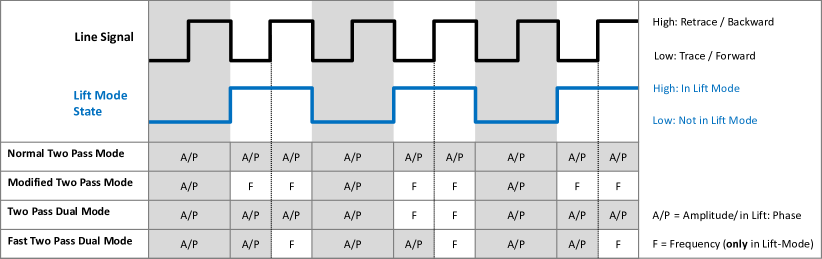
Figure 7: Timing diagram of the modified two-pass mode. Line signal and lift mode state are fed into the micro-controller. Depending on the operation mode (chosen by the user) the drive signal applied to the modulation piezo is switched either to originate from the external lock-in amplifier HF2LI (marked F for frequency in the table) that is measuring frequency shift via a phase-locked loop or kept at the internal lock-in amplifier that is measuring phase shift while in lift mode (notation: A/P for amplitude/phase). Switching is done via CMOS multiplexers, which enable fast and reliable operation.

Signal switching is realised by a home-built switching-box that consist of a micro-controller (µC) controlling several DG409 CMOS analog multiplexers which interconnect the two devices. A timing diagram of the operation can be found in Fig. 7. The line signal (indicating the scan direction i.e. trace/forward or retrace/backward) and the lift mode state is fed into the µC. According to these signals and the selected operation mode, the µC connects the excitation signal either to the build-in lock-in using Q-control or the external HF2LI to drive the modulation piezo. Via a graphical user interface (GUI) the user can modify the µC operation and choose between several different operating modes. The following two modes of operation are of particular interest in the scope of this paper:

• Normal Two-Pass Mode. The well-known and widely used common two-pass operation mode. No switching of signals. Used to obtain a first overlook or non-quantitative measurements in combination with Q-control.

• Fast Two-Pass Dual-Mode. A fast mode where in forward direction phase shift and in backward direction frequency shift is measured. As fast as the normal two-pass mode, however the (redundant) control trace is not available, that may otherwise hint inexperienced users problematic measurements settings (for example inappropriate scan speed that will yield the forward and backward data not equaling each other).

III.3 Signal Improvement

The feasibility of the new two-pass dual-mode is demonstrated by a measurement of a nano-patterned magnetic sample, which combines topography features and low magnetic stray fields. The sample consists of circles with different sizes, here 3 circles with a diameter of $d=300$ nm and height $h=60$ nm have been chosen for evaluation (see Fig. 8 (a) for the sample topography). The sample consists of a Ta(5)/Pt(8)/Co(1)/Ru(1.4)/Pt(0.6)₁₀/Pt(2.4) multilayer stack (numbers in nm) on Si with perpendicular magnetic anisotropy. More details are available in [Fernández Scarioni et al., 2021]. As the measurements were performed in two-pass dual-mode, it is ensured that phase and frequency shift is measured in immediate succession, enabling direct comparability of phase and frequency measurements. A full MFM image obtained by frequency shift measurement in vacuum at Q-factor of $Q\approx 9000$ is portrayed in Fig. 8 (b). As the sample possesses structures with 60 nm topography, the follow slope line mode was used (see Chap. III.5).

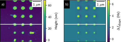
Figure 8: Nanostructured sample. (a) Topography overview. The tree circles with diameter $d=300$ nm (marked by the white line) have been used for the line profiles that are used for evaluation. All structures are 60 nm heigh. Used multilayer system: Ta(5)/Pt(8)/[Co(1)/Ru(1.4)/Pt(0.6)]₁₀/Pt(2.4). (b) Corresponding MFM frequency shift image acquired in vacuum at $Q=9117$.

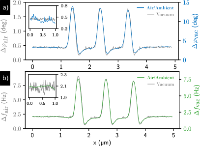
Figure 9: Line profile of the structured magnetic sample in air and vacuum with phase shift and frequency shift signal detection. (a) Phase shift data. Gray profile: Measurement in air with phase shift detection for $Q\approx 170$. Noise contribution is clearly recognizable. Blue profile: Phase shift measurement in vacuum with dampened $Q\approx 1600$. Please note the different scaling on the the y-axes. Improvement in signal originates from the increase of absolute phase data signal, while the noise floor did not enhance. This is visualized by the inset in the top left corner, that zooms into a small excerpt of the signal while using identical y-axis scaling. (b) Frequency shift data. Gray profile: Measurement in air detecting frequency shift, $Q\approx 170$. Dominant noise contribution. Green profile: Vacuum measurement with frequency shift detection, $Q\approx 9000$. Similar scaling on the the y-axes. While the absolute frequency response did not change significantly, the noise decreased drastically. This is visualized by the inset in the top left corner, that zooms into a small excerpt of the signal while using identical y-axis scaling. All measurements have been acquired with a scan rate of 0.05 Hz. Note: Calibration of the piezo scanners in air differs from the calibration in vacuum, thus x has been rescaled to match the calibration. This can be circumvented by issuing and loading a vacuum calibration file when operating in vacuum. The slight asymmetry in the dips is due to the canting angle that has not been corrected for this measurement, as we desired to compare the raw data. Canting angles can be corrected using qMFM routines (that would filter noise in the process).

The results of measurements for different Q-factors are portrayed in Fig. 9. The 4 lineplots show the (a) phase shift signal in air (gray line profile, $Q\approx 170$) and phase shift signal in vacuum (blue line profile, $Q\approx 1600$). In (b) the frequency shift signal in air (gray line profile, $Q\approx 170$) and the frequency shift signal in vacuum (green line profile, $Q\approx 9000$) are plotted.

As expected, in both detection modes the signal improves when operating in vacuum compared to ambient conditions. As discussed in the theory part, the signal improvement for the phase shift measurement originates from the increase in absolute phase shift signal, which is confirmed by the experiment. For the phase-signal, the improvement behaves linearly to the Q-factor (see Table 1 and Fig. 10), increasing the phase-signal $\Delta\varphi=7.4\pm 0.29$ deg every $\Delta Q=100$. However, this is only valid for small $\varphi$, as for phase values that are more than 10 deg away from the phase at resonance, a considerable drop off due to non-linear effects will emerge. Furthermore, the noise-contribution of Q-control increases for rising Q, canceling out the better phase-signal completely, as observable in the SNR values in Table 1. In this specific setup, with this specific cantilever batch, the sweet-spot for phase measurements is around $Q\approx 1000$.

		Q	Noise	Signal	SNR
Frequency	Air	217	9.721 mV	518 mV	56,4
	Vacuum	9117	1.079 mV	552 mV	545
Phase	Air	217	0.028 deg	1.185 deg	42,8
	Vacuum	495	0.014 deg	4.080 deg	291
	Vacuum	1018	0.017 deg	7.753 deg	456
	Vacuum	1491	0.040 deg	10.97 deg	274

Table 1: Comparison of phase and frequency shift measurements in air and vacuum. Q has been calculated from frequency sweep data. The rms noise (root mean square average) is obtained from scans far away from the surface (several 100 µm, e.g. in stray-field free space). The signal describes the peak-to-peak values of the same area of interest (which are the structured magnetic circles, as shown in Fig 9). SNR is calculated out of these values. For the frequency measurements a signal of 100 mV equals a frequency shift of 1,00 Hz. While for rising Q the phase-signal improves linearly, also the noise contribution from Q-control needs to be considered, canceling out the improvement for this specific cantilever at Q-factors at around 1000.

For the frequency shift measurement, the signal amplitude remained constant within the margin of error (as expected), while the noise decreased noticeable. Corresponding values are listed in Table 1. For each measurement situation the quality factor, the root mean square (rms) noise, the maximum measured signal amplitude and corresponding SNR are listed. Note that 100 mV equal a frequency shift of 1,00 Hz in the here presented measurement setup.

While non-linear phase response will become an issue entering double digit degree phase response, limiting the maximum usable Q-factor, for frequency measurements useable Q-factors are only restricted by the cantilever. Another critical advantage is the elimination of non-linear behaviour when using frequency shift that will be demonstrated in the following section.

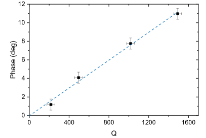
Figure 10: Peak to peak phase signal for rising Q-factors. For small $\varphi$ the improvement behaves linearly to the Q-factor. A slope of $\Delta\varphi=0.74\pm 0.029$ deg every $\Delta Q=100$ can be found. Note that for large Q-factors non-linear effects come into play, causing non-linear effects for large phase shift values (not shown here). Uncertainty bars account for the drift present during the measurement series.

III.4 Elimination of Non-Linearity

The origin of the non-linear behaviour has been extensively discussed before. Here, the effect is demonstrated on a very well known, calculable multilayer reference sample that forms up and down magnetized domains in a maze pattern, that should result in equal areal percentages of bright and dark areas. However, in phase shift measurements for rising Q-factors an increasingly higher areal percentage of dark domains can be observed as shown in Fig. 11. For convenience all images are accompanied by their corresponding histogram. In (a) the domain pattern was measured in ambient conditions ($Q\approx 220$) using phase shift, forming an equal domain distribution. In picture (b) the same reference sample was measured in vacuum ($Q\approx 1800$), using phase shift and Q-control. The Q-factor was chosen as large as possible to illustrate the effect as effectively as possible. The dark domains are much more pronounced, clearly visible in the histogram. Without the prior knowledge of the phase behaviour this could be easily misinterpreted as offset due to electrostatic effects, sample defect, or, even worse, as real measurement data. This can be a great pitfall when interpreting data for material characterisation and quantitative measurements. However, with this setup we can rule out that any electrostatic or sample defect caused this effect, as the fast two-pass dual-mode was used, that is acquiring phase shift in trace and frequency shift in retrace. Image (c) makes use of that setup, showing the exact same position of the sample with the same measurement parameters at the AFM, with the difference that the modulation piezo is now driven by the external lock in amplifier HF2LI. The frequency shift data shows, as expected, equally distributed dark and bright domains. Therefore, the imbalance in the phase shift distribution solely descends from the measurement technique itself.

Figure 11: Measurement of a qMFM reference sample for different Q-factors. The well known, calculable Co/Pt multilayer sample with the layer architecture Pt(2 nm)/[(Co(0.4 nm)/Pt(0.9 nm)]₁₀₀/Pt(5 nm)/Ta(5 nm) on Si is used in this comparison measurement. The sample has been characterized in detail in [Hu et al., ]. While in (a) the domain distribution is even (same amount of bright and dark domains in the image, mirror-symmetry in the histogram) in ambient conditions for low Q-factors, in (b) under vacuum conditions with damped Q-factor ($Q\approx 1800$) and phase shift detection the dark domains get more pronounced, showing distinctly in the histogram as asymmetry. In (c) the to (b) corresponding frequency shift image is plotted (fast two-pass dual-mode $Q\approx 9000$). As the two-pass dual-mode has been used (meaning the sample could not have changed its physical properties in between), this observation cannot be explained to tip sample interaction or any other effects (magnetisation, electric potentials, etc.) and and must originate from the measurement principle itself. To prove the point data in (c) has been run through Eq. 4, yielding image (d). Similar asymmetry (as seen in (b)) with dominant dark domains can be observed.

The origin of the observed non-symmetry of domain distribution can be explained in a straight forward way by Eq. 4 and the corresponding phase curve in Fig. 6. As the setpoint is slightly off peak and therefore in the arctan slightly off point symmetry, positive phase shift values run faster in the non-linear regime providing less signal, thus not only decreasing in absolute values but also breaking the symmetry of the corresponding peaks itself (as clearly observable in the histogram). By running the frequency values of Fig. 11 (c) trough Eq. 4 (with $f_{0}=74660$ Hz and actual operation 30 Hz above $f_{0}$) the corresponding Fig. 11 (d) can be calculated which is corresponding well to the measured data in (b).

Equally the other way round is possible: If the corresponding phase curvature has been acquired in advance, these non-linearities could be compensated in post-processing by correcting the measured phase values with the phase values that would be expected if they could be acquired linearly. However, as the arctan is losing slope when far away from the area of point symmetry, sensitivity is lost. Correcting these values will boost noise to the point where no signal can be recovered anymore. This is highly undesired, thus underlining the usefulness of the new modified two-pass mode.

III.5 Topography interplay

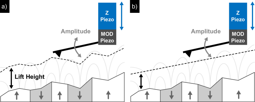
Figure 12: MFM operation in two-pass/lift mode. (a) Second pass with lifted cantilever. The topography of the first pass is retraced. While the short-ranged Lennard-Jones potential cannot influence the cantilever oscillation at this height, the long-ranged magnetic sample stray fields interact with the magnetic tip, shifting the phase of the cantilever oscillation relative to the excitation at the modulation piezo. (b) Second pass that does not retrace the topography but only sample tilt. Useful for flat samples or samples with known structure to eliminate topography interplay in the MFM-signal.

MFM images of structured samples using the common two-pass mode can be misleading as topography can interplay in the magnetic image. In the common operation mode (see Fig. 12 (a)) the surface is retraced in the second pass, including every topography detail. For example, non-magnetic dirt on a flat magnetic sample could be easily mistaken as magnetic signal, as the dirt will cause additional lift height in the second pass, thus moving the cantilever out of the samples stray field and leading to a change in magnetic signal. Also, strong magnetic samples that do not allow a clean topography image without magnetic cross-talk are problematic, as these magnetic details are getting counter-compensated in the second pass.

In particular the issue of topography interplay emerges when pursuing measurements of manufactured structured samples. This can easily demonstrated at the sample at hand, as shown in Fig. 13. When following the topography of the circular structures, at the edges the tip gets very close to the structure, casting a dark shadow (see Fig. 13 (a) and the corresponding grey colored line profile in (c)). However, for simulations and calculations almost always a flat plane above the surface is considered. Thus, a common MFM image that follows the topography can be misleading and pose a pitfall when evaluating data, especially when pursuing quantitative MFM (qMFM).

This problem can be countered by operation in follow slope line mode, as shown in Fig. 12 (b). By fitting a linear slope trough the measured topography (ignoring outliers due to dirt), the samples tilt can be traced in the second pass while ignoring its topography. However, this mode must be carefully operated to not crash the tip into any structure or dirt. It is advisable to image the samples topography beforehand in order to derive a suitable the lift height value. In Fig. 13 (b) (and blue colored line profile in (c)) a lift height of 120 nm was chosen for the follow slope line mode, which equals a lift height of 60 nm in the common (follow topography) mode, as the structures are regarded at outliers. The difference of both traces is quite obvious and corresponds well to the simulated traces in (d). Non-symmetry in the experimental data is attributed to tip tilt that could be compensated in qMFM.

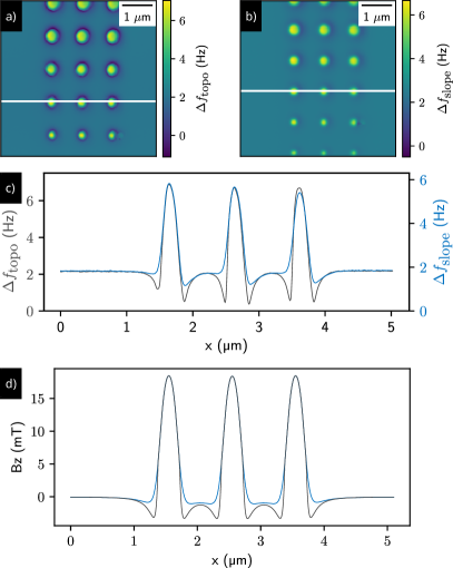
Figure 13: MFM measurements in common lift mode and follow slope line mode. Both measurements where acquired in two-pass dual-mode measuring frequency shift at a Q-factor of $Q\approx 9000$. (a) Commonly used lift mode operation that retraces the samples topography in the lifted pass. The circular structures cast a dark shadow around its edges. (b) Same measurement done in follow slope line mode. The dark shadows decreased, while overall peaks remained constant. (c) Line profiles along the white marked line in the scans for better visualization of effect at hand. Gray: Line profile corresponding to (a). Blue: Line profile corresponding to (b). The dips emerging due to the topography retrace are noticeable less pronounced and solely a measurement artefact. Again, the slight asymmetry in the dips is due to the canting angle that has not been corrected for this measurement, as this is not a qMFM measurement but raw data. (d) Simulated magnetic stray field in z-direction Bz for a constant follow slope lift height of 120 nm (blue) and topography tracing height of 60 nm (black). Even tough without taking the TTF into account, good overall agreement of the effect to (c) is apparent.

IV Summary and Outlook

While common Q-control is a very as useful feature for running amplitude-controlled measurements in vacuum AFM, due to its limitations and non-linear behaviour in phase shift measurements it is not feasible for vacuum MFM. However, these issues can be circumvented by measuring frequency shift instead. Thus, a new two-pass dual-mode was introduced, combining the advantages of both methods into a fast and sensitive vacuum MFM operation mode, capable of handling magnetic samples with topography.

This novel operation mode was realized via a micro-controller that switches the required signal via CMOS multiplexers to an external HF2LI lock-in amplifier to measure frequency shift utilizing a phase-locked loop.

The improved sensitivity of the new operation mode has been demonstrated by MFM-measurements on a nanostructured magnetic sample. The linear response of the measurement technique was investigated using a very well-known calculable multi-layer reference sample, that is forming a domain pattern structure.

With our approach high-sensitivity linear MFM measurements on structured as well as on flat samples are possible using the principle of common two-pass MFM with only small modifications and minimal required user retraining. With that technique a path to high-sensitivity, high-resolution quantitative magnetic force microscopy in vacuum is now available to a broad user base using frequency-based evaluation.

Author Declarations

Conflict of Interest

The authors declare no conflict of interest.

Author Contributions

Christopher Habenschaden: Analysis & Interpretation, Conceptualization, Data Curation, Formal Analysis, Methodology, Software, Validation, Visualization, Writing - Original Draft. Sibylle Sievers: Analysis & Interpretation, Conceptualization, Formal Analysis, Funding Acquisition, Methodology, Project Administration, Resources, Supervision, Validation, Writing - Review & Editing. Alexander Klasen: Validation, Writing - Review & Editing. Andrea Cerreta: Technical support, Validation. Hans Werner Schumacher: Analysis & Interpretation, Conceptualization, Funding Acquisition, Project Administration, Supervision, Validation, Writing - Review & Editing.

Data availability

The data that support the findings of this study are available from the corresponding author upon reasonable request.

References

- (1) X. Hu, G. Dai, S. Sievers, A. Fernández-Scarioni, H. Corte-León, R. Puttock, C. Barton, O. Kazakova, M. Ulvr, P. Klapetek, M. Havlíček, D. Nečas, Y. Tang, V. Neu, and H. W. Schumacher, 511, 166947.
- (2) H. J. Hug, B. Stiefel, P. J. A. van Schendel, A. Moser, R. Hofer, S. Martin, H.-J. Güntherodt, S. Porthun, L. Abelmann, J. C. Lodder, G. Bochi, and R. C. O’Handley, 83, 5609.
- (3) P. J. A. van Schendel, H. J. Hug, B. Stiefel, S. Martin, and H.-J. Güntherodt, 88, 435.
- Zhao et al. (a) X. Zhao, A.-O. Mandru, C. Vogler, M. A. Marioni, D. Suess, and H. J. Hug, 2, 7478 (a).
- (5) Schwenk, Johannes, 10.5451/UNIBAS-006672084.
- Sakar et al. (2021) B. Sakar, S. Sievers, A. Fernández Scarioni, F. Garcia-Sanchez, İ. Öztoprak, H. W. Schumacher, and O. Öztürk, Magnetochemistry 7, 78 (2021).
- Feng et al. (a) Y. Feng, A.-O. Mandru, O. Yıldırım, and H. Hug, 18, 024016 (a).
- IEC (2021) IEC, IEC TS 62607-9-1:2021 (2021).
- (9) K. Babcock, M. Dugas, S. Manalis, and V. Elings, MRS Online Proceedings Library 355, 311.
- Morris (2021) J. Morris, Seagate’s 2021 Virtual Analyst Event (2021).
- (11) S. Luo and L. You, 9, 10.1063/5.0042917.
- Liu et al. (2023) P. Liu, Y. Zhang, K. Li, Y. Li, and Y. Pu, iScience 26, 107584 (2023).
- Feng et al. (b) Y. Feng, P. M. Vaghefi, S. Vranjkovic, M. Penedo, P. Kappenberger, J. Schwenk, X. Zhao, A. O. Mandru, and H. J. Hug, 551, 169073 (b).
- (14) T. R. Albrecht, P. Grütter, D. Horne, and D. Rugar, 69, 668.
- (15) E. Meyer, R. Bennewitz, and H. J. Hug, Scanning Probe Microscopy: The Lab on a Tip (Springer International Publishing).
- (16) J. Schwenk, X. Zhao, M. Bacani, M. A. Marioni, S. Romer, and H. J. Hug, 107, 132407, 1506.07349 .
- Zhao et al. (b) X. Zhao, J. Schwenk, A. O. Mandru, M. Penedo, M. Baćani, M. A. Marioni, and H. J. Hug, 20, 013018 (b).
- (18) B. Voigtländer, Scanning Probe Microscopy: Atomic Force Microscopy and Scanning Tunneling Microscopy (Springer Berlin Heidelberg).
- (19) G. Haugstad, Atomic force microscopy (John Wiley and Sons) includes bibliographical references.
- Kazakova et al. (2019) O. Kazakova, R. Puttock, C. Barton, H. Corte-León, M. Jaafar, V. Neu, and A. Asenjo, Journal of applied Physics 125 (2019).
- Winkler et al. (2023) R. Winkler, M. Ciria, M. Ahmad, H. Plank, and C. Marcuello, Nanomaterials 13, 2585 (2023).
- Rodrıguez and Garcıaa (2003) T. R. Rodrıguez and R. Garcıaa, Applied Physics Letters 82, 4821 (2003).
- (23) H. Hölscher and U. D. Schwarz, 42, 608.
- Note (1) The actual signal response depends on tip and sample. “Weak” samples/tips with small stray magnetic stray fields may not be affected, as their phase response may stay within single digit degrees.
- Fernández Scarioni et al. (2021) A. Fernández Scarioni, C. Barton, H. Corte-León, S. Sievers, X. Hu, F. Ajejas, W. Legrand, N. Reyren, V. Cros, O. Kazakova, and H. Schumacher, Physical Review Letters 126, 077202 (2021).
- Note (2) As for this comparison measurement an air class cantilever was used, the observed Q of around 10 k is far away from the possible limits of 200 k for carefully manufactured high Q vacuum cantilevers.