Systematic integral evaluation for spin-resummed binary dynamics

Abstract

Computation of spin-resummed observables in post-Minkowskian dynamics typically involve evaluation of Feynman integrals deformed by an exponential factor, where the exponent is a linear sum of the momenta being integrated. Such integrals can be viewed as tensor integral generating functions, which provide alternative approaches to tensor reduction of Feynman integrals. We develop a systematic method to evaluate tensor integral generating functions using conventional multiloop integration techniques. The spin-resummed aligned-spin eikonal at second post-Minkowskian order is considered as a phenomenologically relevant example where evaluation of tensor integral generating functions is necessary.

I Introduction

Inspired by quantum field theoretic approaches to gravity Iwasaki (1971); Donoghue (1994); Bjerrum-Bohr et al. (2003); Holstein and Donoghue (2004); Holstein and Ross (2008); Neill and Rothstein (2013); Bjerrum-Bohr et al. (2014); Damour (2018), modern methods to compute scattering amplitude have been widely applied to the study of classical dynamics of binary black hole scattering, from conservative dynamics Bjerrum-Bohr et al. (2018); Cheung et al. (2018); Cristofoli et al. (2019); Bern et al. (2019a, b); Parra-Martinez et al. (2020); Di Vecchia et al. (2020, 2021a, 2021b); Herrmann et al. (2021); Bjerrum-Bohr et al. (2021a, b); Damgaard et al. (2021); Brandhuber et al. (2021a); Bjerrum-Bohr et al. (2022a, b); Bern et al. (2022a, b, 2021a); Damgaard et al. (2023); Di Vecchia et al. (2023); Heissenberg (2023); Adamo and Gonzo (2023) and gravitational bremsstrahlung Kosower et al. (2019); Brandhuber et al. (2023); Herderschee et al. (2023); Elkhidir et al. (2023); Georgoudis et al. (2023); Caron-Huot et al. (2023); Bohnenblust et al. (2023); Bini et al. (2023); Georgoudis et al. (2024a); Adamo et al. (2024); Bini et al. (2024); Alessio and Di Vecchia (2024); Georgoudis et al. (2024b); Brunello and De Angelis (2024) to effects of spin Guevara (2019); Arkani-Hamed et al. (2021); Guevara et al. (2019a); Chung et al. (2019); Guevara et al. (2019b); Arkani-Hamed et al. (2020); Aoude et al. (2020); Chung et al. (2020); Guevara et al. (2021); Chen et al. (2022a); Kosmopoulos and Luna (2021); Chiodaroli et al. (2022); Bautista et al. (2021); Cangemi et al. (2022); Ochirov and Skvortsov (2022); Damgaard et al. (2019); Bern et al. (2021b); Comberiati and de la Cruz (2022); Maybee et al. (2019); Haddad (2022); Chen et al. (2022b); Menezes and Sergola (2022); Febres Cordero et al. (2023); Alessio and Di Vecchia (2022); Bern et al. (2022c); Aoude et al. (2022a, b, 2023); Bautista (2023); De Angelis et al. (2023); Brandhuber et al. (2024); Aoude et al. (2024); Riva et al. (2022); Luna et al. (2023) (see also refs. Antonelli et al. (2019); Damour (2020); Kälin et al. (2020); Dlapa et al. (2022a, b, c); Jakobsen et al. (2023, 2021a); Mougiakakos et al. (2021); Jakobsen et al. (2021b); Mogull et al. (2021); Jakobsen et al. (2022); Vines (2018); Vines et al. (2019); Liu et al. (2021); Jakobsen and Mogull (2022); Damgaard et al. (2022); Bianchi et al. (2023); Gonzo and Shi (2024) for related approaches), motivated in part by the detection of gravitational waves by the LIGO-Virgo collaboration Abbott et al. (2016). The relevant perturbative expansion is the post-Minkowskian (PM) expansion, where general relativistic corrections are added to the unperturbed special relativistic kinematics. The study of PM dynamics is more than a theoretical interest, as they can be used in building waveform models for gravitational wave detection Buonanno et al. (2024).

The typical integrals encountered in the study of PM dynamics can be formulated as Feynman integrals, which can be handled efficiently by modern amplitude techniques such as the integration-by-parts (IBP) reduction Smirnov (2008); Lee (2015); Larsen and Zhang (2016) and the method of differential equations Gehrmann and Remiddi (2000); Kotikov (1991); Henn (2013). The function space of the master integrals and their associated graph topologies were studied for the conservative scattering dynamics at 4PM and 5PM orders Bern et al. (2022a); Dlapa et al. (2022a); Damgaard et al. (2023); Frellesvig et al. (2024a); Driesse et al. (2024); Klemm et al. (2024); Frellesvig et al. (2024b). The function space remains practically the same when spin effects are incorporated perturbatively into the non-spinning dynamics.

However, the function space becomes completely different when exact spin dependence—or spin resummation—is considered. The motivation for studying spin resummation in binary Kerr dynamics is that gravitational wave physics is becoming a precision science; one potential obstruction for high-precision gravitational wave physics is inaccurate modelling of spin effects in gravitational waveform models Dhani et al. (2024), which needs to be improved with better understanding of spin effects in gravitational two-body dynamics.

The spin-induced multipole moments of black holes can be generated by the Newman-Janis shift Newman and Janis (1965); Arkani-Hamed et al. (2020), where the position of the black hole is complexified and shifted in the imaginary spin direction. The translation operator in the imaginary direction is $\exp(i\alpha\cdot\mathbf{\nabla})=\exp(\alpha\cdot K)$, and the same factor appears when the Newman-Janis shift is promoted to a dynamical statement Kim et al. (2024). In particular, the typical Feynman integrals encountered in the context of PM dynamics are modified by exponential factors corresponding to translations along the imaginary spin direction.

Such integrals can be considered in a more general setting as tensor integral generating functions (TIGFs), where a typical Feynman integrand is deformed by an exponential factor of integration variables. The TIGFs provide an alternative route to tensor reduction of Feynman integrals Feng (2023). More importantly, consideration of such integrals allows us to treat the impact parameter space Fourier transform on an equal footing with loop momenta integration, and leads us to new insights on PM dynamics presented in impact parameter space Brunello and De Angelis (2024). For example, the spurious poles from the intermediate loop integral reduction, and computation of the terms that contribute to the loop integrals but vanish under the impact parameter space transform, can be avoided by performing IBP reduction at the full integrand level.

Unfortunately, known multiloop integration techniques are not directly applicable to evaluation of such modified Feynman integrals. We introduce a method to tame the exponential factor and convert it into an extra delta constraint, rendering the integrand suitable for application of conventional multiloop integration techniques. Interestingly, the extra delta constraint leads to significantly different function space of the master integrals when compared to the original master integrals with the same topology.

As a phenomenologically important application, the developed method is used to compute the 2PM spin-resummed eikonal for binary Kerr scattering. To simplify the analysis we consider a generalisation of the aligned spin configuration, where the spin vectors are aligned but allowed to have components along the impact parameter. The minimal coupling three-point amplitude Arkani-Hamed et al. (2021) and the spin-resummed heavy-mass effective field theory (HEFT) Compton amplitude Bjerrum-Bohr et al. (2024, 2023) are used to build the integrand from unitarity cuts Bern et al. (1994, 1995); Bjerrum-Bohr et al. (2003) and heavy-mass/velocity cuts Brandhuber et al. (2021a); Bjerrum-Bohr et al. (2021a, b).

II General methods for tensor integral generating functions

TIGFs are obtained from a typical loop integrand as a deformation by an exponential factor, viz. 

$$\mathcal{I}^{(\alpha)}[\mathbf{y}]:=\int\prod_{j=1}^{L}d^{D}K_{j}\frac{e^{i(\sum_{j=1}^{L}\alpha_{j}\cdot K_{j})}\Big{(}\prod\limits_{k=r+1}^{n}\delta^{\lambda_{k}{-}1}(\mathcal{D}_{k})\Big{)}}{\mathcal{D}_{1}^{\lambda_{1}}\cdots\mathcal{D}_{r}^{\lambda_{r}}}\,,$$ (1)

where $\delta^{\lambda}(x)=\frac{d^{\lambda}}{dx^{\lambda}}\delta(x)$, $(\alpha)=(\alpha_{1}^{\mu},\cdots,\alpha_{L}^{\mu})$ is the vector of arguments, $\mathbf{y}$ is the vector of kinematic invariants and $\mathcal{D}_{i}$ are the inverse propagators; $(K+p)^{2}-m^{2}$ or $2(K\cdot p)$ when eikonalised . In the rest of the letter, we set $D=4-2\epsilon$ for dimensional regularisation. Integrals with non-trivial numerator factors can be obtained from TIGFs as derivative operators of $\alpha_{j}^{\mu}$ acting on them, which is a less-explored tensor reduction method for Feynman integrals Feng (2023). This alternative tensor reduction approach may provide more efficient methods to reduce irreducible numerators, which are one of the bottlenecks in evaluating Feynman integrals.

Some specialised techniques were developed for their reduction and evaluation, including modification of IBP reduction to incorporate the extra exponential factor Feng (2023); Feng et al. (2024); Li et al. (2024); Brunello et al. (2024); Brunello and De Angelis (2024). We take a different route and develop a systematic method to reduce and evaluate TIGFs using conventional multiloop integration techniques. Our key proposal is converting TIGF integrands (1) into a typical Feynman integrand; we introduce an auxiliary parameter $t$ and Fourier transform the exponential factor into a delta constraint,

$$\mathcal{I}^{(\alpha)}[\mathbf{y}] =\int dte^{it}\tilde{\mathcal{I}}^{(\alpha)}[t,\mathbf{y}]\,,$$ (2)

where $\tilde{\mathcal{I}}^{(\alpha)}[t,\mathbf{y}]$ is defined as

$$\int\prod_{j=1}^{L}d^{D}K_{j} \frac{\delta(\sum_{j=1}^{L}\alpha_{j}\cdot K_{j}-t)\Big{(}\prod\limits_{k=r+1}^{s}\delta^{\lambda_{k}{-}1}(\mathcal{D}_{k})\Big{)}}{\mathcal{D}_{1}^{\lambda_{1}}\cdots\mathcal{D}_{r}^{\lambda_{r}}}\,.$$ (3)

$\tilde{\mathcal{I}}^{(\alpha)}[t,\mathbf{y}]$ is a typical Feynman integrand, and conventional IBP reduction can be applied to reduce it to a set of master integrals

$$\tilde{\mathcal{I}}_{1}^{(\alpha)}[t,\mathbf{y}]\,,\,\cdots\,,\,\tilde{\mathcal{I}}_{n}^{(\alpha)}[t,\mathbf{y}]\,.$$ (4)

The conventional method of evaluating master integrals using differential equations applies

$$\begin{aligned} \partial_{t}\tilde{\mathcal{I}}_{i}^{(\alpha)}[t,\mathbf{y}]&=\sum_{j=1}^{n}A_{ij}(t,\mathbf{y})\tilde{\mathcal{I}}_{j}^{(\alpha)}[t,\mathbf{y}]\,,\\ \partial_{y}\tilde{\mathcal{I}}_{i}^{(\alpha)}[t,\mathbf{y}]&=\sum_{j=1}^{n}B_{ij}(t,\mathbf{y})\tilde{\mathcal{I}}_{j}^{(\alpha)}[t,\mathbf{y}]\,.\end{aligned}$$ (5)

An important class of this problem is when the $t$-dependence factorises from the $\mathbf{y}$-dependence so that the differential equations (5) decouple,

$$A_{ij}=A_{ij}(t)\,, B_{ij}=B_{ij}(\mathbf{y})\,,$$ (6)

and spin-resummed PM dynamics falls into this class. In such a case, the $t$-dependence can be factored from the $\mathbf{y}$-dependence,

$$\tilde{\mathcal{I}}_{i}^{(\alpha)}[t,\mathbf{y}]=f_{i}(t)\,\widehat{\mathcal{I}}_{i}^{(\alpha)}[\mathbf{y}]\,,$$ (7)

and the $t$ Fourier integral of (2) factors from the loop integrals, which can be absorbed by normalisation of the effective master integrals $\widehat{\mathcal{I}}_{i}^{(\alpha)}[\mathbf{y}]$. The conventional differential equation approach can be applied to the second set of equations in (5) for evaluation of the effective master integrals $\widehat{\mathcal{I}}_{i}^{(\alpha)}[\mathbf{y}]$. An observable is then given as a linear combination of the effective master integrals.

In the rest of the letter, we apply the aforementioned techniques to the evaluation of spin-resummed one-loop eikonal phase as a concrete phenomenologically relevant example.

III Spin-resummed 2PM eikonal

The classical eikonal can be understood as the generator of scattering observables Gonzo and Shi (2024); Kim et al. (2024), which is computed as the impact-parameter-space Fourier transform of the classical $2\to 2$ one-loop amplitude Brandhuber et al. (2021a). The one-loop HEFT amplitude with classical spin Chen and Wang (2024) is our starting point

$$\leavevmode\hbox to0pt{\vbox to0pt{\text{[drawing]}}}\begin{split}&M_{\rm HEFT}(q,v_{1},v_{2},a_{1},a_{2})={-1\over 2!}\\ &\int{d^{D}\ell_{1}\over(2\pi)^{D-1}}\Big{(}{\delta(2m_{2}\ell_{1}{\cdot}v_{2})\over\ell_{1}^{2}\ell_{2}^{2}}M_{a_{2}}(\ell_{1},v_{2})\\ &\phantom{as}\times M_{a_{2}}(\ell_{2},v_{2})\,M_{a_{1}}(\ell_{1},\ell_{2},v_{2})\Big{)}\,,\end{split} v_{1} v_{2} \ell_{1} \ell_{2} v_{1} v_{2} \ell_{1} \ell_{2}$$ (8)

where $\ell_{2}=q-\ell_{1}$. $M_{a_{2}}$ and $M_{a_{1}}$ are the three-point and four-point HEFT amplitudes provided in the appendix.

The key ingredient is the HEFT Compton amplitude Bjerrum-Bohr et al. (2023, 2024), which—contrary to the minimal coupling Compton amplitude Arkani-Hamed et al. (2021)—is free of unphysical singularities. However, the amplitude has spurious singularities entering through the entire functions

$$G_{1}(x_{1})G_{1}(x_{2}) ={\sinh(x_{1})\over x_{1}}{\sinh(x_{2})\over x_{2}}\,,$$ (9)

$$G_{2}(x_{1},x_{2}) ={1\over x_{2}}\Big{(}{\sinh(x_{12})\over x_{12}}-\cosh(x_{2}){\sinh(x_{1})\over x_{1}}\Big{)}\,,$$

where $x_{12}=x_{1}+x_{2}$ and $x_{i}=a_{1}{\cdot}\ell_{i}$.

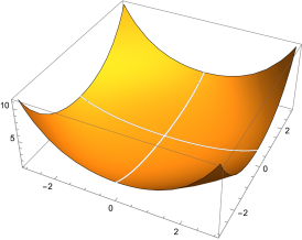
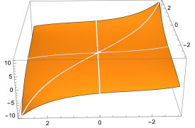
Figure 1: $G_{1}(x_{1})G_{1}(x_{2})$ (left) and $G_{2}(x_{1},x_{2})$ (right)

As can be seen from the graph of the two functions in fig. 1, the apparent singularities of (9) do not correspond to actual singularities. Nevertheless, the spurious singularities can be problematic in the evaluation of the integrals, especially when the integrations are performed numerically as the singularities spoil numerical stability. We therefore introduce their integral representations

$$G_{1}(x_{1})G_{1}(x_{2}) =\int_{0}^{1}d\sigma_{1}d\sigma_{2}\cosh(\sigma_{1}x_{1})\cosh(\sigma_{2}x_{2})\,,$$

$$G_{2}(x_{1},x_{2}) =\int_{0}^{1}d\sigma_{1}d\sigma_{2}\Big{(}\sigma_{1}\sinh\left(\sigma_{1}x_{1}+\sigma_{1}\sigma_{2}x_{2}\right)$$

$$\leavevmode\nobreak\ \leavevmode\nobreak\ \leavevmode\nobreak\ \leavevmode\nobreak\ \leavevmode\nobreak\ \leavevmode\nobreak\ \leavevmode\nobreak\ \leavevmode\nobreak\ -\sinh\left(\sigma_{2}x_{2}\right)\cosh\left(\sigma_{1}x_{1}\right)\Big{)}\,,$$ (10)

which removes spurious denominators at the price of auxiliary integrations over $\sigma_{i}$. Analogous integral representations are used for $G_{1}$ functions appearing in the three-point amplitudes when constructing the integrand (8).

The eikonal $\chi$ is obtained by transforming the HEFT amplitude to impact parameter space

$$\begin{aligned} \chi&=\int{d^{D}q\over(2\pi)^{D-2}}{e^{iq{\cdot}b}\delta(q{\cdot}v_{1})\delta(q{\cdot}v_{2})\over 4m_{1}m_{2}}\\ &\phantom{=asdfasdf}\times M_{\rm HEFT}(q,v_{1},v_{2},a_{1},a_{2})\,.\end{aligned}$$ (11)

We focus on a slight generalisation of the aligned spin configuration of a binary Kerr system; $a^{\mu}\equiv a_{1}^{\mu}=\xi a_{2}^{\mu}$ and $v_{1}{\cdot}a_{2}=v_{2}{\cdot}a_{1}=0$ with $a{\cdot}b\neq 0$.

Exchanging the order of integration to pull out the $\sigma_{i}$ integrals, the eikonal can be schematically written as

$$\chi=\int_{0}^{1}\prod_{j=1}^{4}d\sigma_{j}\sum_{\alpha}\mathcal{I}^{(\alpha)}[\mathbf{y}]\,,$$ (12)

where

$$y_{1} =v_{1}{\cdot}v_{2}\,, y_{2} ={a{\cdot}a\over-b{\cdot}b}\,, y_{3} =b{\cdot}b\,, y_{4} ={b{\cdot}a\over-b{\cdot}b}\,$$ (13)

are the Lorentz scalars the eikonal depends on. The integral representation (III) reorganises the original integrand as a sum over integrands of the form (1) with additional numerator factors, which we classify into distinct sectors $(\alpha)$ defined by the exponential factor $\exp(iq{\cdot}\hat{b}+i\ell_{1}{\cdot}\hat{a})$.

$$(\alpha) \equiv(\hat{b}\,,\,\hat{a})$$ (14)

$$\equiv(b+c^{\prime}_{1}(\sigma)\tilde{a}_{1}+c^{\prime}_{2}(\sigma)\tilde{a}_{2}\,,\,c^{\prime}_{3}(\sigma)\tilde{a}_{1}+c^{\prime}_{4}(\sigma)\tilde{a}_{2})\,,$$

$$(\mathbf{y}) =(y_{1}\,,\,\hat{y}_{2}\,,\,\hat{y}_{3}\,,\,\hat{y}_{4}\,,\,\sigma_{1}\,,\,\sigma_{2}\,,\,\sigma_{3}\,,\,\sigma_{4})\,,$$

$$(K_{1},K_{2}) =(q\,,\,\ell_{1})\,.$$

The Lorentz scalars $\hat{y}_{i}$ are defined similar to (13) with hatted variables $\hat{b},\hat{a}$. The tilded spin vectors $\tilde{a}_{j}^{\mu}=ia_{j}^{\mu}$ are analytic continuation of the real spin(-length) vectors of the black holes $a_{j}^{\mu}$. After evaluation, the master integrals can be analytically continued back to real spin.

After employing the methods developed in the previous section, a typical integrand for a given sector $(\alpha)$ takes the form

$$\mathcal{I}^{(\alpha)}[\mathbf{y}]=\int_{-\infty}^{\infty}dte^{it}\int{d^{D}qd^{D}\ell_{1}\over(2\pi)^{2D-3}}\delta(q{\cdot}\hat{b}+\ell_{1}{\cdot}\hat{a}-t)$$ (15)

$$\times{\delta(q{\cdot}v_{1})\delta(q{\cdot}v_{2})\delta(\ell_{1}{\cdot}v_{2})\over 8m_{1}m^{2}_{2}\,\ell_{1}^{2}(q-\ell_{1})^{2}}\Big{(}\sum_{r=0}^{2}{N^{(r)}(\mathbf{y})\over(\ell_{1}{\cdot}v_{1})^{r}}+{N^{(3)}(\mathbf{y})\over q^{2}}\Big{)}\,,$$

where denominators of the integrand were kept explicit. The relevant topologies are given in fig. 2. Each sector can be reduced to master integrals by applying conventional multiloop integration techniques such as IBP reduction.

Figure 2: The graph topologies of master integrals, edges labelled by $\lambda_{r}$ defined in (22). The dashed line is the delta constraint originating from the exponential factor. The thick lines are remaining delta constraints, while the thin lines are physical propagators.

All master integrals satisfy the factorisation condition (6). Moreover, solving the differential equations in $t$ yields power-law $t$-dependence of the master integrals. All terms resulting from reducing (15) have $t$-dependence of the form

$${t^{j-4\epsilon}\over\epsilon}\,, j\in[0,6]\,.$$ (16)

As remarked, the contributions from the $t$ Fourier transform can be treated as a constant factor. It is remarked that the divergent $\frac{1}{\epsilon}$ term in dimensional regularisation vanishes under the $t$ Fourier transform, therefore the constant factor is finite.

An exemplary term in the $N^{(3)}$ category is

$$\mathcal{I}_{ex}[\mathbf{y}]=\int{d^{D}qd^{D}\ell_{1}\over(2\pi)^{2D-3}}e^{iq{\cdot}b}{\delta(q{\cdot}v_{1})\delta(q{\cdot}v_{2})\delta(\ell_{1}{\cdot}v_{2})\over\ell_{1}^{2}(q-\ell_{1})^{2}q^{2}}$$ (17)

$$\times\frac{(16\pi G_{N})^{2}m_{1}m_{2}^{2}\left(\ell_{1}{\cdot}v_{1}\right){}^{2}\cosh\left((1-\xi)a_{1}{\cdot}q+2\xi a_{1}{\cdot}\ell_{1}\right)}{16}\,.$$

The $\cosh$ function splits the integrand into two sectors; sector $(1)=(\hat{a}_{1},\hat{b}_{1})=(2\tilde{a}_{1}\xi\,,\,\tilde{a}_{1}(1-\xi)+b)$ and sector $(2)=(\hat{a}_{2},\hat{b}_{2})=(-2\tilde{a}_{1}\xi\,,\,\tilde{a}_{1}(\xi-1)+b)$. Each sector reduces to three master integrals by IBP reduction,

$$\mathcal{I}^{(\alpha)}_{ex}[\mathbf{y}]=-(16\pi G_{N})^{2}{\pi\over 2}\frac{m_{1}m_{2}^{2}(y_{1}^{2}-1)}{32\hat{y}_{2}\hat{y}_{3}}$$ (18)

$$\phantom{as}\times\Big{(}2\hat{y}_{3}\left(\hat{y}_{2}+2\hat{y}_{4}-1\right)\widehat{\mathcal{I}}_{1}^{(\alpha)}[\mathbf{y}]+2\widehat{\mathcal{I}}_{2}^{(\alpha)}[\mathbf{y}]+\widehat{\mathcal{I}}_{3}^{(\alpha)}[\mathbf{y}]\Big{)}\,,$$

where the master integrals are defined by (21) and the superscript $(\alpha)$ denotes the sectors. (17) becomes

$$\mathcal{I}_{ex}[\mathbf{y}]=\mathcal{I}^{(1)}_{ex}[\mathbf{y}]+\mathcal{I}^{(2)}_{ex}[\mathbf{y}]\,,$$ (19)

where each $\mathcal{I}^{(\alpha)}_{ex}[\mathbf{y}]$ is complex but the sum $\mathcal{I}_{ex}[\mathbf{y}]$ is real.

The integrals in (12) reduce to 320 sectors. Each sector has five master integrals. However, only three master integrals per sector appear in the final result,

$$\chi =\int_{0}^{1}\prod_{j=1}^{4}d\sigma_{j}\sum_{\alpha=1}^{320}\Big{(}c_{1,\alpha}(\mathbf{y})\widehat{\cal I}^{(\alpha)}_{1}[\mathbf{y}]+c_{2,\alpha}(\mathbf{y})\widehat{\cal I}^{(\alpha)}_{2}[\mathbf{y}]$$

$$\leavevmode\nobreak\ \leavevmode\nobreak\ \leavevmode\nobreak\ \leavevmode\nobreak\ \leavevmode\nobreak\ \leavevmode\nobreak\ \leavevmode\nobreak\ \leavevmode\nobreak\ \leavevmode\nobreak\ \leavevmode\nobreak\ \leavevmode\nobreak\ \leavevmode\nobreak\ \leavevmode\nobreak\ \leavevmode\nobreak\ \leavevmode\nobreak\ \leavevmode\nobreak\ \leavevmode\nobreak\ \leavevmode\nobreak\ \leavevmode\nobreak\ \leavevmode\nobreak\ \leavevmode\nobreak\ \leavevmode\nobreak\ \leavevmode\nobreak\ \leavevmode\nobreak\ \leavevmode\nobreak\ \leavevmode\nobreak\ \leavevmode\nobreak\ \leavevmode\nobreak\ +c_{3,\alpha}(\mathbf{y})\widehat{\cal I}^{(\alpha)}_{3}[\mathbf{y}]\Big{)}\,,$$ (20)

where the master integrals are

$$\widehat{\cal I}^{(\alpha)}_{1}[\mathbf{y}] ={D-4\over t^{2D-8}}J^{(\alpha)}_{1,1,1,1,1,1,0,0}\,,$$

$$\widehat{\cal I}^{(\alpha)}_{2}[\mathbf{y}] ={1\over t^{2D-10}}J^{(\alpha)}_{2,1,1,1,1,1,0,0}\,,$$

$$\widehat{\cal I}^{(\alpha)}_{3}[\mathbf{y}] ={1\over t^{2D-10}}J^{(\alpha)}_{1,1,1,1,1,1,0,1}\,,$$ (21)

defined as

$$J^{(\alpha)}_{\lambda_{1},\lambda_{2},\lambda_{3},\lambda_{4},\lambda_{5},\lambda_{6},\lambda_{7},\lambda_{8}}\equiv\int{d^{D}qd^{D}\ell_{1}\over(2\pi)^{2D-3}}\delta^{\lambda_{6}-1}(\hat{a}{\cdot}\ell_{1}+\hat{b}{\cdot}q-t)$$

$$\phantom{asdfasdf}\times{\delta^{\lambda_{3}-1}(\ell_{1}{\cdot}v_{2})\delta^{\lambda_{4}-1}(q{\cdot}v_{1})\delta^{\lambda_{5}-1}(q{\cdot}v_{2})\over(\ell_{1}^{2})^{\lambda_{1}}((q-\ell_{1})^{2})^{\lambda_{2}}(\ell_{1}{\cdot}v_{1})^{\lambda_{7}}(q^{2})^{\lambda_{8}}}\,.$$ (22)

The numerators $N^{(0,1,2)}$ of (12) reduce to $\widehat{\cal I}^{(\alpha)}_{1,2}[\mathbf{y}]$, while the numerators $N^{(3)}$ of (12) reduce to $\widehat{\cal I}^{(\alpha)}_{1,2,3}[\mathbf{y}]$. The integrals $\widehat{\cal I}^{(\alpha)}_{1,2}[\mathbf{y}]$ correspond to the left topology of fig. 2, while the integral $\widehat{\cal I}^{(\alpha)}_{3}[\mathbf{y}]$ corresponds to the right topology of fig. 2. The apparent $t$-dependence in (21) makes the master integrals $\widehat{\cal I}^{(\alpha)}_{1,2,3}[\mathbf{y}]$ independent of $t$. As mentioned previously, the other two master integrals, $J^{(\alpha)}_{1,1,1,2,1,1,0,0}$ and $J^{(\alpha)}_{1,1,1,1,1,1,1,0}$, never appear and their evaluation is unnecessary for evaluating the eikonal. It is also remarked that both $c_{j,\alpha}(\mathbf{y})$ and $\widehat{\cal I}^{(\alpha)}_{j}[\mathbf{y}]$ are finite in dimensional regularisation.

The final result for the eikonal phase is available in the public repository KerrEikonal2pm Chen et al. (2024). We emphasise that the result contains all-orders-in-spin contributions for the generalised aligned spin configuration with $a{\cdot}b\neq 0$.

IV Evaluation of the Master integrals

We evaluate the master integrals using the method of differential equations Gehrmann and Remiddi (2000); Kotikov (1991); Henn (2013). The $\hat{y}_{3}$-dependence of the master integrals can be determined from dimensional analysis, since the only dimensionful variable is $\hat{y}_{3}$. Moreover, the differential operator $\partial_{y_{1}}$ is diagonal in the system of master integrals, and the $y_{1}$-dependence of the master integrals can be solved separately.

The nontrivial systems of differential equations are given by $\hat{y}_{2,4}$. The two systems are degenerate for the master integrals $\widehat{\mathcal{I}}_{1,2}$ and they only depend on the combination $\hat{y}_{2}^{\prime}=\hat{y}_{2}+2\hat{y}_{4}$. The differential equations over $\hat{y}_{2}^{\prime}$ for $\widehat{\mathcal{I}}_{1,2}$ are solved by complete elliptic integrals ,

$$\widehat{\mathcal{I}}_{1}[\mathbf{y}] =\frac{C}{\sqrt{-\hat{y}_{3}}\sqrt{y_{1}^{2}-1}}\,\frac{K(\hat{y}_{2}^{\prime})}{\pi}\,,$$

$$\widehat{\mathcal{I}}_{2}[\mathbf{y}] =-\frac{C\sqrt{-\hat{y}_{3}}}{\sqrt{y_{1}^{2}-1}}\,\frac{(\hat{y}_{2}^{\prime}-1)K(\hat{y}_{2}^{\prime})+E(\hat{y}_{2}^{\prime})}{\pi}\,,$$ (23)

where the integration constant $C=-\frac{1}{16\pi^{2}}$ is fixed from the spinless limit $\hat{y}_{2}^{\prime}\to 0$.

The differential equations satisfied by $\widehat{\mathcal{I}}_{3}$ are

$$\partial_{\hat{y}^{\prime}_{2}}\widehat{\mathcal{I}}_{3}[\mathbf{y}]={-1\over 2\left(\hat{y}^{\prime}_{2}-2\hat{y}_{4}\right)\left(\hat{y}^{\prime}_{2}+\hat{y}^{2}_{4}-2\hat{y}_{4}\right)}\times$$

$$\Big{(}\hat{y}_{4}^{2}\widehat{\mathcal{I}}_{3}[\mathbf{y}]-\frac{C}{\pi}\frac{(\sqrt{-\hat{y}_{3}})}{\sqrt{y_{1}^{2}-1}}\left(\hat{y}^{\prime}_{2}+2\hat{y}_{4}\left(\hat{y}_{4}-1\right)\right)E\left(\hat{y}^{\prime}_{2}\right)$$

$$+\frac{C}{\pi}\frac{(\sqrt{-\hat{y}_{3}})}{\sqrt{y_{1}^{2}-1}}\left(1-\hat{y}_{4}\right)\left(\hat{y}^{\prime}_{2}-2\hat{y}_{4}\right)K\left(\hat{y}^{\prime}_{2}\right)\Big{)}\,,$$ (24)

$$\partial_{\hat{y}_{4}}\widehat{\mathcal{I}}_{3}[\mathbf{y}]={1\over\left(\hat{y}^{\prime}_{2}-2\hat{y}_{4}\right)\left(\hat{y}^{\prime}_{2}+\hat{y}^{2}_{4}-2\hat{y}_{4}\right)}\Big{(}\hat{y}_{4}\left(\hat{y}^{\prime}_{2}-\hat{y}_{4}\right)\widehat{\mathcal{I}}_{3}[\mathbf{y}]$$

$$-C\frac{(\sqrt{-\hat{y}_{3}})}{\sqrt{y_{1}^{2}-1}}\left(\hat{y}^{\prime}_{2}-1\right)\left(\hat{y}^{\prime}_{2}-2\hat{y}_{4}\right)K\left(\hat{y}^{\prime}_{2}\right)$$

$$-C\frac{(\sqrt{-\hat{y}_{3}})}{\sqrt{y_{1}^{2}-1}}\left(\hat{y}_{4}\hat{y}^{\prime}_{2}+\hat{y}^{\prime}_{2}-2\hat{y}_{4}\right)E\left(\hat{y}^{\prime}_{2}\right)\Big{)}\,.$$ (25)

The common denominator factor in the two equations implies that the master integral should be understood as an integral over the elliptic curve

$${\cal Y}^{2}=(\hat{y}^{\prime}_{2}-2z)(z^{2}-2z+\hat{y}^{\prime}_{2})\,,$$ (26)

where $z$ is the integration variable to be identified as $-\hat{y}_{4}$ after integration. $\widehat{\mathcal{I}}_{3}[\mathbf{y}]$ is computed by solving (24) at $\hat{y}_{4}=0$, which yields the boundary value for the remaining integration over $\hat{y}_{4}$. Carrying out the $\hat{y}_{4}$ integration, we have

$$\widehat{\mathcal{I}}_{3}[\mathbf{y}] =\frac{C(\sqrt{-\hat{y}_{3}})}{\sqrt{y_{1}^{2}-1}}\frac{\sqrt{\hat{y}^{\prime}_{2}+\hat{y}_{4}\left(\hat{y}_{4}-2\right)}}{\sqrt{\hat{y}^{\prime}_{2}-2\hat{y}_{4}}}\Bigg{[}\frac{2E(\hat{y}^{\prime}_{2})+\pi}{2\pi}$$

$$\phantom{=a}+\int_{0}^{\hat{y}_{4}}dz\Big{(}\frac{\left(1-\hat{y}^{\prime}_{2}\right)\left(\hat{y}^{\prime}_{2}-2z\right)K\left(\hat{y}^{\prime}_{2}\right)}{\pi\,{\cal Y}\,(z^{2}-2z+\hat{y}^{\prime}_{2})}$$ (27)

$$\phantom{=asdfasdfasdf}-\frac{\left(\hat{y}^{\prime}_{2}z-2z+\hat{y}^{\prime}_{2}\right)E\left(\hat{y}^{\prime}_{2}\right)}{\pi\,{\cal Y}\,(z^{2}-2z+\hat{y}^{\prime}_{2})}\Big{)}\Bigg{]}\,.$$

The $z$-integral can be reduced by the IBP relations following from the exact differentials

$$d\left(\frac{\hat{y}^{\prime}_{2}-2z}{{\cal Y}}\right)\,,\,d\left(\frac{(\hat{y}^{\prime}_{2}-2z)^{2}}{{\cal Y}}\right)\,.$$ (28)

Eliminating integrals with undesired denominators, we arrive at

$$\widehat{\mathcal{I}}_{3}[\mathbf{y}] =\,\frac{C\sqrt{-\hat{y}_{3}}}{\sqrt{y_{1}^{2}-1}}\Bigg{[}\frac{\sqrt{\hat{y}^{\prime}_{2}+\hat{y}_{4}^{2}-2\hat{y}_{4}}}{\pi\sqrt{\hat{y}^{\prime}_{2}-2\hat{y}_{4}}}\Big{(}{\pi-2K(\hat{y}^{\prime}_{2})\over 2}$$

$$-\left(E(\hat{y}^{\prime}_{2})-K(\hat{y}^{\prime}_{2})\right)\int_{0}^{\hat{y}_{4}}\frac{dz}{{\cal Y}}-K(\hat{y}^{\prime}_{2})\int_{0}^{\hat{y}_{4}}\frac{zdz}{{\cal Y}}\Big{)}$$

$$+\,\frac{E(\hat{y}^{\prime}_{2})+\left(1-\hat{y}_{4}\right)K(\hat{y}^{\prime}_{2})}{\pi}\Bigg{]}\,,$$ (29)

where the integrals can be converted to incomplete elliptic integrals, which can be evaluated to arbitrary numerical precision. The integration constants were fixed by requiring regularity of the spin expansion around $\hat{a}^{\mu}=0$. Since $\hat{a}^{\mu}\to 0$ is a singular limit of the underlying curve (26), we expand (IV) around $\hat{y}_{4}$ first and then expand in $\hat{y}_{2}$ to obtain the series expansion of $\widehat{\mathcal{I}}_{3}$. The master integrals $\widehat{\mathcal{I}}_{1,2,3}$ were checked against brute-force calculations based on the formulas in appendix B of ref. Kim et al. (2024), and found to agree up to $\mathcal{O}(\hat{a}^{20})$.

V Results

The eikonal phase (III) is exact to all orders in spin, and can be expanded in spin before the $\sigma_{j}$-integration for a check against perturbative-in-spin calculations. The spin-expanded $\sigma_{j}$ integrand turns out to be polynomial in $\sigma_{j}$, and the auxiliary $\sigma_{j}$ integrals can be evaluated exactly. We provide files for evaluating the spin-expanded $\sigma_{j}$ integrand in the public repository KerrEikonal2pm Chen et al. (2024). We have checked that (III) expanded to $\mathcal{O}(a^{8})$ is consistent with the results of ref. Chen and Wang (2024).

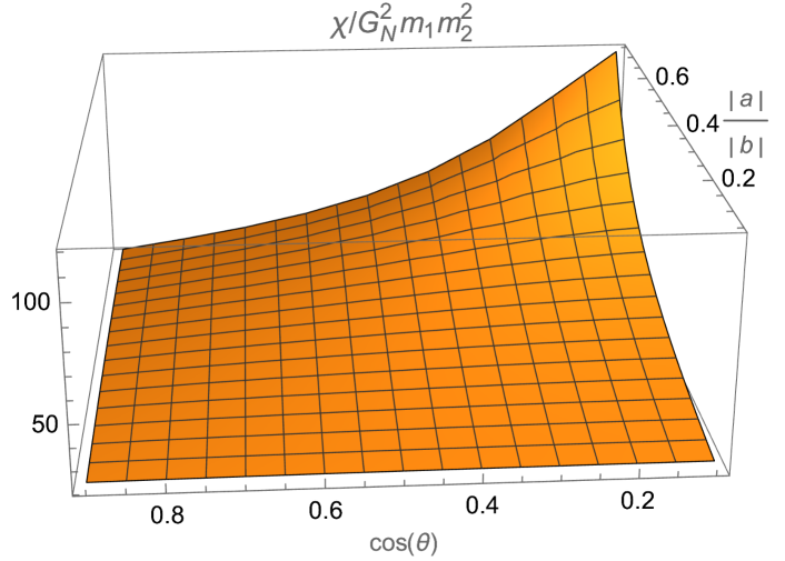
Figure 3: The eikonal (III) as a function of ${|a|\over|b|}$ and $\cos(\theta)=\frac{-a\cdot b}{|a||b|}$ with numerical errors $\sim 10^{-15}$.

The merit of the eikonal phase (III) is that we can study its full spin dependence quantitatively, since the $\sigma_{j}$ integrations can be numerically evaluated with high precision. As an example of numerically studying the eikonal (III), we consider the scattering of a test Kerr black hole on a Schwarzschild background, corresponding to the substitution

$$\chi_{a_{2}=0}=\chi|_{\xi\rightarrow 0}\,,$$ (30)

which is presented in fig. 3. The parameters $y_{1}={12\over 10}$ and $y_{3}=-1$ are chosen for the ranges $|\sqrt{-y_{2}}|<0.75$ and $\cos(\theta)\in[0,0.9]$, where $\theta$ denotes the angle between $a^{\mu}$ and $b^{\mu}$ such that $\sqrt{-y_{2}}\cos(\theta)=y_{4}$.

The numerical calculations can be tested against analytic predictions. For example, the 2PM aligned-spin ($\cos(\theta)=0$) eikonal is expected to have the singularity $\propto(|b|^{2}-|a|^{2})^{-3/2}$ based on analytic studies Damgaard et al. (2022); Aoude et al. (2022a); Kim et al. (2024). Fig. 4 shows numerical evaluation of (III) in the aligned-spin configuration plotted against the reference curve $\frac{\beta}{(|b|^{2}-|a|^{2})^{3/2}}$, where the constant $\beta$ was fit to (III) at $|b|=1.02\,|a|$ and other unspecified parameters are the same as in fig. 3. The two lines on fig. 4 show a good agreement near the singular point $|b|=|a|$, having $\lesssim 5\,\%$ relative difference for $|b|\leq 1.04\,|a|$. This singularity can be interpreted as the dynamics detecting the ring singularity from spin resummation, since the eikonal has a singularity only at $|b|=0$ when spin is treated perturbatively.

Figure 4: Aligned-spin $\chi$ near the singular point $|b|=|a|$. The reference $\frac{\beta}{(|b|^{2}-|a|^{2})^{3/2}}$ intersects at $|b|=1.02\,|a|$.

VI Conclusions and outlook

In this letter, a systematic method to reduce and evaluate TIGFs was introduced and applied to the scattering dynamics of a binary Kerr system in the generalised aligned-spin configuration. The corresponding 2PM eikonal phase (III) was presented in a closed form, which can be studied analytically by expanding to arbitrary orders in spin, or can be studied numerically through numerical integrations for exact spin dependence.

An important application of TIGFs is generation of tensor integrals, directly providing an alternative method of performing tensor reduction in Feynman integrals Feng (2023). The approach may prove useful for reduction of irreducible numerators, which in many cases becomes a bottleneck when evaluation of multiloop Feynman integrals are involved. In this regard, understanding the criteria for the factorisation of the $t$-dependence (e.g. from intersection theory Cho and Matsumoto (1995); Mastrolia and Mizera (2019); Frellesvig et al. (2019); Brunello and De Angelis (2024)) will be important, as the factorisation played a crucial role in obtaining closed-form expressions for the TIGFs considered.

Another future direction to explore would be the study of function space complexity for TIGFs. We have seen that elliptic integrals appear in effective two-loop (2PM) topologies for TIGFs (see also ref. Kim et al. (2024) for electromagnetism). It is reasonable to expect that more complex functions (e.g. elliptic multi-polylogarithms Broedel et al. (2018), integrals over Calabi-Yau manifolds Bourjaily et al. (2022)) will appear in effective three-loop (3PM) graph topologies when integrals are deformed into TIGFs. Moreover, we can attempt to quantify the increase in transcendentality of the function space when typical Feynman integrals are deformed into TIGFs. This may even lead to an exploration of new geometries that have not yet been associated with Feynman integrals.

Special cases of TIGFs appear ubiquitously in quantum-field-theory-inspired approaches to classical gravitating systems, especially in the calculation of scattering waveforms Brandhuber et al. (2023); Herderschee et al. (2023); Elkhidir et al. (2023); Georgoudis et al. (2023); Caron-Huot et al. (2023); Bohnenblust et al. (2023); Bini et al. (2023); Georgoudis et al. (2024a); Adamo et al. (2024); Bini et al. (2024); Alessio and Di Vecchia (2024); Georgoudis et al. (2024b); Brunello and De Angelis (2024). It would also be interesting to apply the developed methods to these problems.

Coming back to the initial motivation for the study of TIGFs, it would be interesting to apply the developed methods to 3PM all-orders-in-spin dynamics and study spin resummation. Whether we have the exact three-graviton-Kerr five-point amplitude—which is necessary for constructing the 3PM integrand—is less relevant, as long as the conjectured five-point amplitude correctly captures features of the dynamical Newman-Janis shift; we expect the singularity structures of the binary Kerr dynamics to be governed by the dynamical Newman-Janis shift, and correct singularity structures are the most important when we attempt to resum the perturbative two-body dynamics Kim et al. (2024). Compared to the 2PM dynamics studied in this letter, the spin-resummed 3PM dynamics is qualitatively different in that it is the first order where next-to-leading-order effects in the mass-ratio expansion enters into the dynamics Vines et al. (2019), thereby including the first beyond background-probe limit effects. The insights gained from studying singularity structures of spin-resummed binary Kerr dynamics may motivate new resummation schemes for spinning binary dynamics, providing a more accurate incorporation of spin effects in waveform models used by gravitational wave observatories, potentially having far-reaching consequences for astrophysics and multi-messenger astronomy.

Appendix A Appendix: The Compton amplitude

The three point amplitude with one graviton momentum $p_{1}^{\mu}$ and classical black hole spin $a^{\mu}$ Guevara et al. (2019a); Chung et al. (2019); Arkani-Hamed et al. (2020); Aoude et al. (2020); Johansson and Ochirov (2019); Bjerrum-Bohr et al. (2023) is

$$M_{3}(p_{1}{\cdot}a)=\sqrt{32\pi G_{N}}\,(\bar{p}{\cdot}\varepsilon_{1})(w_{1}{\cdot}\varepsilon_{1})\,,$$ (31)

where $\bar{p}^{\mu}=mv^{\mu}$ denotes massive particle’s momentum,

$$\begin{split}w_{1}^{\mu}&\coloneqq\cosh(p_{1}{\cdot}a)\,\bar{p}^{\mu}-i\frac{\sinh(p_{1}{\cdot}a)}{p_{1}{\cdot}a}(p_{1}{\cdot}S)^{\mu}\,,\end{split}$$ (32)

and $(p_{1}{\cdot}S)^{\mu}=p_{1\nu}S^{\nu\mu}$. The $S^{\mu\nu}$ denotes the spin tensor $S^{\mu\nu}=-\epsilon^{\mu\nu\rho\sigma}\bar{p}_{\rho}a_{\sigma}$.

The Compton amplitude with graviton momenta $p_{1,2}$ is constructed from the double copy Bern et al. (2008, 2010), kinematic Hopf algebra Brandhuber et al. (2021b, 2022a, 2022b), and classical spin bootstrap Bjerrum-Bohr et al. (2024, 2023),

$${M_{4}\over 32\pi G_{N}}=-\Big{(}\!\frac{\bar{p}{\cdot}F_{1}{\cdot}F_{2}{\cdot}\bar{p}}{p_{2}{\cdot}\bar{p}}\Big{)}\Bigg{(}\frac{w_{1}{\cdot}F_{1}{\cdot}F_{2}{\cdot}w_{2}}{2(p_{1}{\cdot}p_{2})(p_{1}{\cdot}\bar{p})}-\frac{p_{1}{\cdot}\bar{p}-p_{2}{\cdot}\bar{p}}{4(p_{1}{\cdot}p_{2})(p_{1}{\cdot}\bar{p})}\Big{(}iG_{2}\left(x_{1},x_{2}\right)(a{\cdot}F_{1}{\cdot}F_{2}{\cdot}S{\cdot}p_{2})+iG_{2}(x_{1},x_{2})(a{\cdot}F_{2}{\cdot}F_{1}{\cdot}S{\cdot}p_{1})$$

$$+iG_{1}\left(x_{12}\right)\text{tr}\left(F_{1}{\cdot}S{\cdot}F_{2}\right)+G_{1}(x_{1})G_{1}(x_{2})\big{(}(a{\cdot}F_{1}{\cdot}\bar{p})(a{\cdot}F_{2}{\cdot}p_{1})\!-\!(a{\cdot}F_{1}{\cdot}p_{2})(a{\cdot}F_{2}{\cdot}\bar{p})-\!\frac{p_{2}{\cdot}\bar{p}\!-\!p_{1}{\cdot}\bar{p}}{2}(a{\cdot}F_{1}{\cdot}F_{2}{\cdot}a)\big{)}\Big{)}\Bigg{)}\,$$

$$+\!{\Big{(}(\partial_{x_{1}}\!-\!\partial_{x_{2}})G_{1}(x_{1})G_{1}(x_{2})\Big{)}\over 4(\bar{p}{\cdot}p_{1})(\bar{p}{\cdot}p_{2})}\Big{(}\bar{p}{\cdot}p_{2}(\bar{p}^{2}(a{\cdot}F_{1}{\cdot}F_{2}{\cdot}a)(a{\cdot}F_{2}{\cdot}F_{1}{\cdot}\bar{p})+a^{2}(\bar{p}_{4}{\cdot}F_{1}{\cdot}F_{2}{\cdot}\bar{p})(a{\cdot}F_{1}{\cdot}F_{2}{\cdot}\bar{p}))\!-\!(1\leftrightarrow 2)\!\Big{)}$$

$$+\Big{(}{i(\partial_{x_{1}}\!-\!\partial_{x_{2}})G_{2}(x_{1},x_{2})\over 4(\bar{p}{\cdot}p_{1})(\bar{p}{\cdot}p_{2})}\Big{)}\Big{(}(\bar{p}{\cdot}p_{2})(a{\cdot}F_{2}{\cdot}F_{1}{\cdot}\bar{p})((a{\cdot}F_{2}{\cdot}\bar{p})(a{\cdot}\widetilde{F}_{1}{\cdot}\bar{p}){-}(a{\cdot}F_{1}{\cdot}\bar{p})(a{\cdot}\widetilde{F}_{2}{\cdot}\bar{p}))+(1\leftrightarrow 2)\Big{)}$$

$$+\!\Big{(}\!{(\partial_{x_{1}}\!-\!\partial_{x_{2}})^{2}\over 2!}{G_{1}(x_{1})}{G_{1}(x_{2})}\Big{)}\Big{(}(a{\cdot}F_{1}{\cdot}\bar{p})(a{\cdot}F_{2}{\cdot}\bar{p})(a{\cdot}F_{1}{\cdot}F_{2}{\cdot}a)\!-\!{a^{2}\over 2}((a{\cdot}F_{1}{\cdot}F_{2}{\cdot}p)(a{\cdot}F_{2}{\cdot}F_{1}{\cdot}\bar{p})-(a{\cdot}F_{1}{\cdot}F_{2}{\cdot}a)(\bar{p}{\cdot}F_{1}{\cdot}F_{2}{\cdot}\bar{p}))\!\Big{)}$$

$$\!\!\!+\Big{(}{i(\partial_{x_{1}}-\partial_{x_{2}})^{2}\over 2!}{G_{2}(x_{1},x_{2})}\Big{)}\Big{(}\!-{1\over 2}\big{(}(a{\cdot}F_{1}{\cdot}F_{2}{\cdot}a)(a{\cdot}F_{2}{\cdot}\bar{p})(a{\cdot}\widetilde{F}_{1}{\cdot}\bar{p})\!-\!(1\leftrightarrow 2)\big{)}\Big{)}\,,$$ (33)

where $x_{i}=a{\cdot}p_{i}$, $F_{i}^{\mu\nu}=p^{\mu}_{i}\varepsilon^{\nu}_{i}-\varepsilon^{\mu}_{i}p^{\nu}_{i}$, and $\widetilde{F}^{\mu\nu}=\frac{1}{2}\epsilon^{\mu\nu\rho\sigma}F_{\rho\sigma}$. The differences between this Compton amplitude and other proposals Cangemi et al. (2023); Bautista et al. (2023) stem from the differences in their respective formalisms and assumptions Bjerrum-Bohr et al. (2023, 2024), which are inherited by the one-loop amplitude Chen and Wang (2024). The recursion relation for the integral representation of the $G$ functions is

$$G_{1}(x_{1}) {=}\int_{0}^{1}d\sigma_{1}\cosh(\sigma_{1}x_{1})\,,$$ (34)

$$G_{2}(x_{1},x_{2}) {=}\int_{0}^{1}d\sigma_{2}\Big{[}\partial_{x_{1}}G_{1}(x_{1}+\sigma_{2}x_{2})$$

$$\leavevmode\nobreak\ \leavevmode\nobreak\ \leavevmode\nobreak\ \leavevmode\nobreak\ \leavevmode\nobreak\ \leavevmode\nobreak\ \leavevmode\nobreak\ \leavevmode\nobreak\ \leavevmode\nobreak\ -\sinh(\sigma_{2}x_{2})\cosh(\sigma_{1}x_{1})\Big{]}\,,$$ (35)

$$G_{r}(x_{1},...,x_{r}) {=}{\int_{0}^{1}}d\sigma_{r}\Big{[}\partial_{x_{1}}G_{r-1}(x_{1}{+}\sigma_{r}x_{r},x_{2},...,x_{r-1})$$

$$-G_{r-1}(x_{1},...,x_{r-1})\sinh(\sigma_{r}x_{r})\Big{]}\,.$$ (36)

References

- Iwasaki (1971) Y. Iwasaki, Prog. Theor. Phys. 46, 1587 (1971).
- Donoghue (1994) J. F. Donoghue, Phys. Rev. D 50, 3874 (1994), arXiv:gr-qc/9405057 .
- Bjerrum-Bohr et al. (2003) N. E. J. Bjerrum-Bohr, J. F. Donoghue, and B. R. Holstein, Phys. Rev. D 67, 084033 (2003), [Erratum: Phys.Rev.D 71, 069903 (2005)], arXiv:hep-th/0211072 .
- Holstein and Donoghue (2004) B. R. Holstein and J. F. Donoghue, Phys. Rev. Lett. 93, 201602 (2004), arXiv:hep-th/0405239 [hep-th] .
- Holstein and Ross (2008) B. R. Holstein and A. Ross, (2008), arXiv:0802.0716 [hep-ph] .
- Neill and Rothstein (2013) D. Neill and I. Z. Rothstein, Nucl. Phys. B877, 177 (2013), arXiv:1304.7263 [hep-th] .
- Bjerrum-Bohr et al. (2014) N. E. J. Bjerrum-Bohr, J. F. Donoghue, and P. Vanhove, JHEP 02, 111 (2014), arXiv:1309.0804 [hep-th] .
- Damour (2018) T. Damour, Phys. Rev. D97, 044038 (2018), arXiv:1710.10599 [gr-qc] .
- Bjerrum-Bohr et al. (2018) N. E. J. Bjerrum-Bohr, P. H. Damgaard, G. Festuccia, L. Plante, and P. Vanhove, Phys. Rev. Lett. 121, 171601 (2018), arXiv:1806.04920 [hep-th] .
- Cheung et al. (2018) C. Cheung, I. Z. Rothstein, and M. P. Solon, Phys. Rev. Lett. 121, 251101 (2018), arXiv:1808.02489 [hep-th] .
- Cristofoli et al. (2019) A. Cristofoli, N. E. J. Bjerrum-Bohr, P. H. Damgaard, and P. Vanhove, Phys. Rev. D 100, 084040 (2019), arXiv:1906.01579 [hep-th] .
- Bern et al. (2019a) Z. Bern, C. Cheung, R. Roiban, C.-H. Shen, M. P. Solon, and M. Zeng, Phys. Rev. Lett. 122, 201603 (2019a), arXiv:1901.04424 [hep-th] .
- Bern et al. (2019b) Z. Bern, C. Cheung, R. Roiban, C.-H. Shen, M. P. Solon, and M. Zeng, JHEP 10, 206 (2019b), arXiv:1908.01493 [hep-th] .
- Parra-Martinez et al. (2020) J. Parra-Martinez, M. S. Ruf, and M. Zeng, JHEP 11, 023 (2020), arXiv:2005.04236 [hep-th] .
- Di Vecchia et al. (2020) P. Di Vecchia, C. Heissenberg, R. Russo, and G. Veneziano, Phys. Lett. B 811, 135924 (2020), arXiv:2008.12743 [hep-th] .
- Di Vecchia et al. (2021a) P. Di Vecchia, C. Heissenberg, R. Russo, and G. Veneziano, Phys. Lett. B 818, 136379 (2021a), arXiv:2101.05772 [hep-th] .
- Di Vecchia et al. (2021b) P. Di Vecchia, C. Heissenberg, R. Russo, and G. Veneziano, JHEP 07, 169 (2021b), arXiv:2104.03256 [hep-th] .
- Herrmann et al. (2021) E. Herrmann, J. Parra-Martinez, M. S. Ruf, and M. Zeng, JHEP 10, 148 (2021), arXiv:2104.03957 [hep-th] .
- Bjerrum-Bohr et al. (2021a) N. E. J. Bjerrum-Bohr, P. H. Damgaard, L. Planté, and P. Vanhove, Phys. Rev. D 104, 026009 (2021a), arXiv:2104.04510 [hep-th] .
- Bjerrum-Bohr et al. (2021b) N. E. J. Bjerrum-Bohr, P. H. Damgaard, L. Planté, and P. Vanhove, (2021b), arXiv:2105.05218 [hep-th] .
- Damgaard et al. (2021) P. H. Damgaard, L. Plante, and P. Vanhove, JHEP 11, 213 (2021), arXiv:2107.12891 [hep-th] .
- Brandhuber et al. (2021a) A. Brandhuber, G. Chen, G. Travaglini, and C. Wen, JHEP 10, 118 (2021a), arXiv:2108.04216 [hep-th] .
- Bjerrum-Bohr et al. (2022a) N. E. J. Bjerrum-Bohr, L. Planté, and P. Vanhove, JHEP 03, 071 (2022a), arXiv:2111.02976 [hep-th] .
- Bjerrum-Bohr et al. (2022b) N. E. J. Bjerrum-Bohr, L. Planté, and P. Vanhove, (2022b), arXiv:2212.08957 [hep-th] .
- Bern et al. (2022a) Z. Bern, J. Parra-Martinez, R. Roiban, M. S. Ruf, C.-H. Shen, M. P. Solon, and M. Zeng, Phys. Rev. Lett. 128, 161103 (2022a), arXiv:2112.10750 [hep-th] .
- Bern et al. (2022b) Z. Bern, J. Parra-Martinez, R. Roiban, M. S. Ruf, C.-H. Shen, M. P. Solon, and M. Zeng, PoS LL2022, 051 (2022b).
- Bern et al. (2021a) Z. Bern, J. Parra-Martinez, R. Roiban, M. S. Ruf, C.-H. Shen, M. P. Solon, and M. Zeng, Phys. Rev. Lett. 126, 171601 (2021a), arXiv:2101.07254 [hep-th] .
- Damgaard et al. (2023) P. H. Damgaard, E. R. Hansen, L. Planté, and P. Vanhove, (2023), arXiv:2307.04746 [hep-th] .
- Di Vecchia et al. (2023) P. Di Vecchia, C. Heissenberg, R. Russo, and G. Veneziano, (2023), arXiv:2306.16488 [hep-th] .
- Heissenberg (2023) C. Heissenberg, (2023), arXiv:2308.11470 [hep-th] .
- Adamo and Gonzo (2023) T. Adamo and R. Gonzo, JHEP 05, 088 (2023), arXiv:2212.13269 [hep-th] .
- Kosower et al. (2019) D. A. Kosower, B. Maybee, and D. O’Connell, JHEP 02, 137 (2019), arXiv:1811.10950 [hep-th] .
- Brandhuber et al. (2023) A. Brandhuber, G. R. Brown, G. Chen, S. De Angelis, J. Gowdy, and G. Travaglini, JHEP 06, 048 (2023), arXiv:2303.06111 [hep-th] .
- Herderschee et al. (2023) A. Herderschee, R. Roiban, and F. Teng, JHEP 06, 004 (2023), arXiv:2303.06112 [hep-th] .
- Elkhidir et al. (2023) A. Elkhidir, D. O’Connell, M. Sergola, and I. A. Vazquez-Holm, (2023), arXiv:2303.06211 [hep-th] .
- Georgoudis et al. (2023) A. Georgoudis, C. Heissenberg, and I. Vazquez-Holm, JHEP 06, 126 (2023), arXiv:2303.07006 [hep-th] .
- Caron-Huot et al. (2023) S. Caron-Huot, M. Giroux, H. S. Hannesdottir, and S. Mizera, (2023), arXiv:2308.02125 [hep-th] .
- Bohnenblust et al. (2023) L. Bohnenblust, H. Ita, M. Kraus, and J. Schlenk, (2023), arXiv:2312.14859 [hep-th] .
- Bini et al. (2023) D. Bini, T. Damour, and A. Geralico, Phys. Rev. D 108, 124052 (2023), arXiv:2309.14925 [gr-qc] .
- Georgoudis et al. (2024a) A. Georgoudis, C. Heissenberg, and R. Russo, JHEP 03, 089 (2024a), arXiv:2312.07452 [hep-th] .
- Adamo et al. (2024) T. Adamo, R. Gonzo, and A. Ilderton, JHEP 05, 034 (2024), arXiv:2402.00124 [hep-th] .
- Bini et al. (2024) D. Bini, T. Damour, S. De Angelis, A. Geralico, A. Herderschee, R. Roiban, and F. Teng, (2024), arXiv:2402.06604 [hep-th] .
- Alessio and Di Vecchia (2024) F. Alessio and P. Di Vecchia, (2024), arXiv:2402.06533 [hep-th] .
- Georgoudis et al. (2024b) A. Georgoudis, C. Heissenberg, and R. Russo, Phys. Rev. D 109, 106020 (2024b), arXiv:2402.06361 [hep-th] .
- Brunello and De Angelis (2024) G. Brunello and S. De Angelis, (2024), arXiv:2403.08009 [hep-th] .
- Guevara (2019) A. Guevara, JHEP 04, 033 (2019), arXiv:1706.02314 [hep-th] .
- Arkani-Hamed et al. (2021) N. Arkani-Hamed, T.-C. Huang, and Y.-t. Huang, JHEP 11, 070 (2021), arXiv:1709.04891 [hep-th] .
- Guevara et al. (2019a) A. Guevara, A. Ochirov, and J. Vines, JHEP 09, 056 (2019a), arXiv:1812.06895 [hep-th] .
- Chung et al. (2019) M.-Z. Chung, Y.-T. Huang, J.-W. Kim, and S. Lee, JHEP 04, 156 (2019), arXiv:1812.08752 [hep-th] .
- Guevara et al. (2019b) A. Guevara, A. Ochirov, and J. Vines, Phys. Rev. D100, 104024 (2019b), arXiv:1906.10071 [hep-th] .
- Arkani-Hamed et al. (2020) N. Arkani-Hamed, Y.-t. Huang, and D. O’Connell, JHEP 01, 046 (2020), arXiv:1906.10100 [hep-th] .
- Aoude et al. (2020) R. Aoude, K. Haddad, and A. Helset, JHEP 05, 051 (2020), arXiv:2001.09164 [hep-th] .
- Chung et al. (2020) M.-Z. Chung, Y.-t. Huang, J.-W. Kim, and S. Lee, JHEP 05, 105 (2020), arXiv:2003.06600 [hep-th] .
- Guevara et al. (2021) A. Guevara, B. Maybee, A. Ochirov, D. O’connell, and J. Vines, JHEP 03, 201 (2021), arXiv:2012.11570 [hep-th] .
- Chen et al. (2022a) W.-M. Chen, M.-Z. Chung, Y.-t. Huang, and J.-W. Kim, JHEP 08, 148 (2022a), arXiv:2111.13639 [hep-th] .
- Kosmopoulos and Luna (2021) D. Kosmopoulos and A. Luna, JHEP 07, 037 (2021), arXiv:2102.10137 [hep-th] .
- Chiodaroli et al. (2022) M. Chiodaroli, H. Johansson, and P. Pichini, JHEP 02, 156 (2022), arXiv:2107.14779 [hep-th] .
- Bautista et al. (2021) Y. F. Bautista, A. Guevara, C. Kavanagh, and J. Vines, (2021), arXiv:2107.10179 [hep-th] .
- Cangemi et al. (2022) L. Cangemi, M. Chiodaroli, H. Johansson, A. Ochirov, P. Pichini, and E. Skvortsov, (2022), arXiv:2212.06120 [hep-th] .
- Ochirov and Skvortsov (2022) A. Ochirov and E. Skvortsov, Phys. Rev. Lett. 129, 241601 (2022), arXiv:2207.14597 [hep-th] .
- Damgaard et al. (2019) P. H. Damgaard, K. Haddad, and A. Helset, JHEP 11, 070 (2019), arXiv:1908.10308 [hep-ph] .
- Bern et al. (2021b) Z. Bern, A. Luna, R. Roiban, C.-H. Shen, and M. Zeng, Phys. Rev. D 104, 065014 (2021b), arXiv:2005.03071 [hep-th] .
- Comberiati and de la Cruz (2022) F. Comberiati and L. de la Cruz, (2022), arXiv:2212.09259 [hep-th] .
- Maybee et al. (2019) B. Maybee, D. O’Connell, and J. Vines, JHEP 12, 156 (2019), arXiv:1906.09260 [hep-th] .
- Haddad (2022) K. Haddad, Phys. Rev. D 105, 026004 (2022), arXiv:2109.04427 [hep-th] .
- Chen et al. (2022b) W.-M. Chen, M.-Z. Chung, Y.-t. Huang, and J.-W. Kim, JHEP 12, 058 (2022b), arXiv:2205.07305 [hep-th] .
- Menezes and Sergola (2022) G. Menezes and M. Sergola, JHEP 10, 105 (2022), arXiv:2205.11701 [hep-th] .
- Febres Cordero et al. (2023) F. Febres Cordero, M. Kraus, G. Lin, M. S. Ruf, and M. Zeng, Phys. Rev. Lett. 130, 021601 (2023), arXiv:2205.07357 [hep-th] .
- Alessio and Di Vecchia (2022) F. Alessio and P. Di Vecchia, Phys. Lett. B 832, 137258 (2022), arXiv:2203.13272 [hep-th] .
- Bern et al. (2022c) Z. Bern, D. Kosmopoulos, A. Luna, R. Roiban, and F. Teng, (2022c), arXiv:2203.06202 [hep-th] .
- Aoude et al. (2022a) R. Aoude, K. Haddad, and A. Helset, Phys. Rev. Lett. 129, 141102 (2022a), arXiv:2205.02809 [hep-th] .
- Aoude et al. (2022b) R. Aoude, K. Haddad, and A. Helset, JHEP 07, 072 (2022b), arXiv:2203.06197 [hep-th] .
- Aoude et al. (2023) R. Aoude, K. Haddad, and A. Helset, Phys. Rev. D 108, 024050 (2023), arXiv:2304.13740 [hep-th] .
- Bautista (2023) Y. F. Bautista, (2023), arXiv:2304.04287 [hep-th] .
- De Angelis et al. (2023) S. De Angelis, R. Gonzo, and P. P. Novichkov, (2023), arXiv:2309.17429 [hep-th] .
- Brandhuber et al. (2024) A. Brandhuber, G. R. Brown, G. Chen, J. Gowdy, and G. Travaglini, JHEP 02, 026 (2024), arXiv:2310.04405 [hep-th] .
- Aoude et al. (2024) R. Aoude, K. Haddad, C. Heissenberg, and A. Helset, Phys. Rev. D 109, 036007 (2024), arXiv:2310.05832 [hep-th] .
- Riva et al. (2022) M. M. Riva, F. Vernizzi, and L. K. Wong, Phys. Rev. D 106, 044013 (2022), arXiv:2205.15295 [hep-th] .
- Luna et al. (2023) A. Luna, N. Moynihan, D. O’Connell, and A. Ross, (2023), arXiv:2312.09960 [hep-th] .
- Antonelli et al. (2019) A. Antonelli, A. Buonanno, J. Steinhoff, M. van de Meent, and J. Vines, Phys. Rev. D 99, 104004 (2019), arXiv:1901.07102 [gr-qc] .
- Damour (2020) T. Damour, Phys. Rev. D 102, 124008 (2020), arXiv:2010.01641 [gr-qc] .
- Kälin et al. (2020) G. Kälin, Z. Liu, and R. A. Porto, Phys. Rev. Lett. 125, 261103 (2020), arXiv:2007.04977 [hep-th] .
- Dlapa et al. (2022a) C. Dlapa, G. Kälin, Z. Liu, and R. A. Porto, Phys. Lett. B 831, 137203 (2022a), arXiv:2106.08276 [hep-th] .
- Dlapa et al. (2022b) C. Dlapa, G. Kälin, Z. Liu, and R. A. Porto, Phys. Rev. Lett. 128, 161104 (2022b), arXiv:2112.11296 [hep-th] .
- Dlapa et al. (2022c) C. Dlapa, G. Kälin, Z. Liu, J. Neef, and R. A. Porto, (2022c), arXiv:2210.05541 [hep-th] .
- Jakobsen et al. (2023) G. U. Jakobsen, G. Mogull, J. Plefka, B. Sauer, and Y. Xu, (2023), arXiv:2306.01714 [hep-th] .
- Jakobsen et al. (2021a) G. U. Jakobsen, G. Mogull, J. Plefka, and J. Steinhoff, Phys. Rev. Lett. 126, 201103 (2021a), arXiv:2101.12688 [gr-qc] .
- Mougiakakos et al. (2021) S. Mougiakakos, M. M. Riva, and F. Vernizzi, Phys. Rev. D 104, 024041 (2021), arXiv:2102.08339 [gr-qc] .
- Jakobsen et al. (2021b) G. U. Jakobsen, G. Mogull, J. Plefka, and J. Steinhoff, (2021b), arXiv:2106.10256 [hep-th] .
- Mogull et al. (2021) G. Mogull, J. Plefka, and J. Steinhoff, JHEP 02, 048 (2021), arXiv:2010.02865 [hep-th] .
- Jakobsen et al. (2022) G. U. Jakobsen, G. Mogull, J. Plefka, and J. Steinhoff, JHEP 01, 027 (2022), arXiv:2109.04465 [hep-th] .
- Vines (2018) J. Vines, Class. Quant. Grav. 35, 084002 (2018), arXiv:1709.06016 [gr-qc] .
- Vines et al. (2019) J. Vines, J. Steinhoff, and A. Buonanno, Phys. Rev. D 99, 064054 (2019), arXiv:1812.00956 [gr-qc] .
- Liu et al. (2021) Z. Liu, R. A. Porto, and Z. Yang, JHEP 06, 012 (2021), arXiv:2102.10059 [hep-th] .
- Jakobsen and Mogull (2022) G. U. Jakobsen and G. Mogull, Phys. Rev. Lett. 128, 141102 (2022), arXiv:2201.07778 [hep-th] .
- Damgaard et al. (2022) P. H. Damgaard, J. Hoogeveen, A. Luna, and J. Vines, Phys. Rev. D 106, 124030 (2022), arXiv:2208.11028 [hep-th] .
- Bianchi et al. (2023) M. Bianchi, C. Gambino, and F. Riccioni, JHEP 08, 188 (2023), arXiv:2306.08969 [hep-th] .
- Gonzo and Shi (2024) R. Gonzo and C. Shi, (2024), arXiv:2405.09687 [hep-th] .
- Abbott et al. (2016) B. P. Abbott et al. (LIGO Scientific, Virgo), Phys. Rev. Lett. 116, 061102 (2016), arXiv:1602.03837 [gr-qc] .
- Buonanno et al. (2024) A. Buonanno, G. Mogull, R. Patil, and L. Pompili, (2024), arXiv:2405.19181 [gr-qc] .
- Smirnov (2008) A. Smirnov, JHEP 10, 107 (2008), arXiv:0807.3243 [hep-ph] .
- Lee (2015) R. N. Lee, JHEP 04, 108 (2015), arXiv:1411.0911 [hep-ph] .
- Larsen and Zhang (2016) K. J. Larsen and Y. Zhang, Phys. Rev. D 93, 041701 (2016), arXiv:1511.01071 [hep-th] .
- Gehrmann and Remiddi (2000) T. Gehrmann and E. Remiddi, Nuclear Physics B 580, 485 (2000).
- Kotikov (1991) A. V. Kotikov, Phys. Lett. B 254, 158 (1991).
- Henn (2013) J. M. Henn, Phys. Rev. Lett. 110, 251601 (2013), arXiv:1304.1806 [hep-th] .
- Frellesvig et al. (2024a) H. Frellesvig, R. Morales, and M. Wilhelm, Phys. Rev. Lett. 132, 201602 (2024a), arXiv:2312.11371 [hep-th] .
- Driesse et al. (2024) M. Driesse, G. U. Jakobsen, G. Mogull, J. Plefka, B. Sauer, and J. Usovitsch, (2024), arXiv:2403.07781 [hep-th] .
- Klemm et al. (2024) A. Klemm, C. Nega, B. Sauer, and J. Plefka, (2024), arXiv:2401.07899 [hep-th] .
- Frellesvig et al. (2024b) H. Frellesvig, R. Morales, and M. Wilhelm, (2024b), arXiv:2405.17255 [hep-th] .
- Dhani et al. (2024) A. Dhani, S. Völkel, A. Buonanno, H. Estelles, J. Gair, H. P. Pfeiffer, L. Pompili, and A. Toubiana, (2024), arXiv:2404.05811 [gr-qc] .
- Newman and Janis (1965) E. T. Newman and A. I. Janis, J. Math. Phys. 6, 915 (1965).
- Kim et al. (2024) J.-H. Kim, J.-W. Kim, and S. Lee, (2024), arXiv:2405.17056 [hep-th] .
- Feng (2023) B. Feng, Commun. Theor. Phys. 75, 025203 (2023), arXiv:2209.09517 [hep-ph] .
- Bjerrum-Bohr et al. (2024) N. E. J. Bjerrum-Bohr, G. Chen, and M. Skowronek, Phys. Rev. Lett. 132, 191603 (2024), arXiv:2309.11249 [hep-th] .
- Bjerrum-Bohr et al. (2023) N. E. J. Bjerrum-Bohr, G. Chen, and M. Skowronek, JHEP 06, 170 (2023), arXiv:2302.00498 [hep-th] .
- Bern et al. (1994) Z. Bern, L. J. Dixon, D. C. Dunbar, and D. A. Kosower, Nucl. Phys. B425, 217 (1994), arXiv:hep-ph/9403226 [hep-ph] .
- Bern et al. (1995) Z. Bern, L. J. Dixon, D. C. Dunbar, and D. A. Kosower, Nucl. Phys. B435, 59 (1995), arXiv:hep-ph/9409265 [hep-ph] .
- Note (1) Although generating functions are usually defined by real exponents, imaginary exponents were used to avoid factors of when solving for the integrals. Such an analytic continuation is known in the probability literature as characteristic functions. This analytic continuation is allowed since Feynman integrals should be understood as generalised functions which may not be well-defined by conventional definitions of integrals.
- Note (2) The delta constraints can be converted to denominators through the distributional identity and its derivatives, therefore they can be considered as propagator factors.
- Feng et al. (2024) B. Feng, C. Hu, J. Shen, and Y. Zhang, (2024), arXiv:2403.16040 [hep-ph] .
- Li et al. (2024) T. Li, Y. Song, and L. Zhang, (2024), arXiv:2404.04644 [hep-ph] .
- Brunello et al. (2024) G. Brunello, G. Crisanti, M. Giroux, P. Mastrolia, and S. Smith, Phys. Rev. D 109, 094047 (2024), arXiv:2311.14432 [hep-th] .
- Chen and Wang (2024) G. Chen and T. Wang, (2024), arXiv:2406.09086 [hep-th] .
- Chen et al. (2024) G. Chen, J.-W. Kim, and T. Wang, “https://github.com/amplitudegravity/kerreikonal2pm,” (2024).
- Note (3) We adopt Mathematica’s definition for the elliptic integrals.
- Cho and Matsumoto (1995) K. Cho and K. Matsumoto, Nagoya Mathematical Journal 139, 67 (1995).
- Mastrolia and Mizera (2019) P. Mastrolia and S. Mizera, JHEP 02, 139 (2019), arXiv:1810.03818 [hep-th] .
- Frellesvig et al. (2019) H. Frellesvig, F. Gasparotto, S. Laporta, M. K. Mandal, P. Mastrolia, L. Mattiazzi, and S. Mizera, JHEP 05, 153 (2019), arXiv:1901.11510 [hep-ph] .
- Broedel et al. (2018) J. Broedel, C. Duhr, F. Dulat, and L. Tancredi, JHEP 05, 093 (2018), arXiv:1712.07089 [hep-th] .
- Bourjaily et al. (2022) J. L. Bourjaily et al., in Snowmass 2021 (2022) arXiv:2203.07088 [hep-ph] .
- Johansson and Ochirov (2019) H. Johansson and A. Ochirov, JHEP 09, 040 (2019), arXiv:1906.12292 [hep-th] .
- Bern et al. (2008) Z. Bern, J. J. M. Carrasco, and H. Johansson, Phys. Rev. D78, 085011 (2008), arXiv:0805.3993 [hep-ph] .
- Bern et al. (2010) Z. Bern, J. J. M. Carrasco, and H. Johansson, Phys. Rev. Lett. 105, 061602 (2010), arXiv:1004.0476 [hep-th] .
- Brandhuber et al. (2021b) A. Brandhuber, G. Chen, G. Travaglini, and C. Wen, JHEP 07, 047 (2021b), arXiv:2104.11206 [hep-th] .
- Brandhuber et al. (2022a) A. Brandhuber, G. Chen, H. Johansson, G. Travaglini, and C. Wen, Phys. Rev. Lett. 128, 121601 (2022a), arXiv:2111.15649 [hep-th] .
- Brandhuber et al. (2022b) A. Brandhuber, G. R. Brown, G. Chen, J. Gowdy, G. Travaglini, and C. Wen, JHEP 12, 101 (2022b), arXiv:2208.05886 [hep-th] .
- Cangemi et al. (2023) L. Cangemi, M. Chiodaroli, H. Johansson, A. Ochirov, P. Pichini, and E. Skvortsov, (2023), arXiv:2312.14913 [hep-th] .
- Bautista et al. (2023) Y. F. Bautista, G. Bonelli, C. Iossa, A. Tanzini, and Z. Zhou, (2023), arXiv:2312.05965 [hep-th] .